A Comparison of Two Tree Detection Methods for Estimation of Forest Stand and Ecological Variables from Airborne LiDAR Data in Central European Forests


Abstract
:
1. Introduction
2. Materials and Methods
2.1. Estimation of Forest Stand Variables from Ground Reference Data
2.2. Estimation of Forest Stand Variables from ALS Data
2.2.1. Individual Tree and Tree Height Detection
2.2.2. Classification of Tree Species Groups
2.2.3. Tree Diameter Derivation
2.2.4. Tree Volume Derivation
2.2.5. Calculation of Forest Stand and Ecological Variables
2.3. Accuracy Assessment
2.3.1. Forest Stands Level
2.3.2. Forest Unit Level
3. Results
3.1. Forest Stands Level
3.2. Forest Unit Level
4. Discussion
4.1. Mean Height
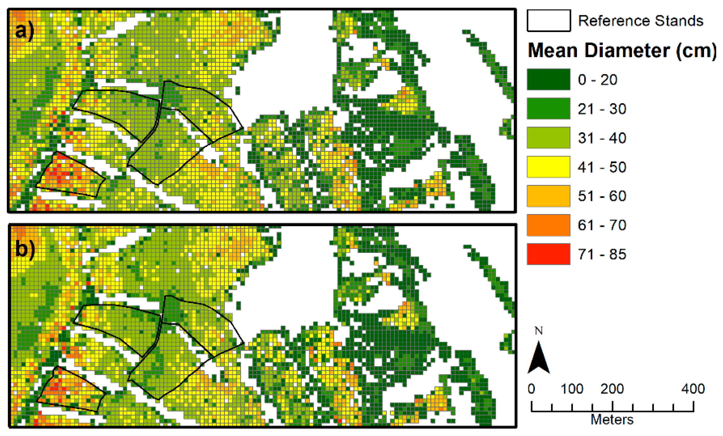
4.2. Mean Diameter
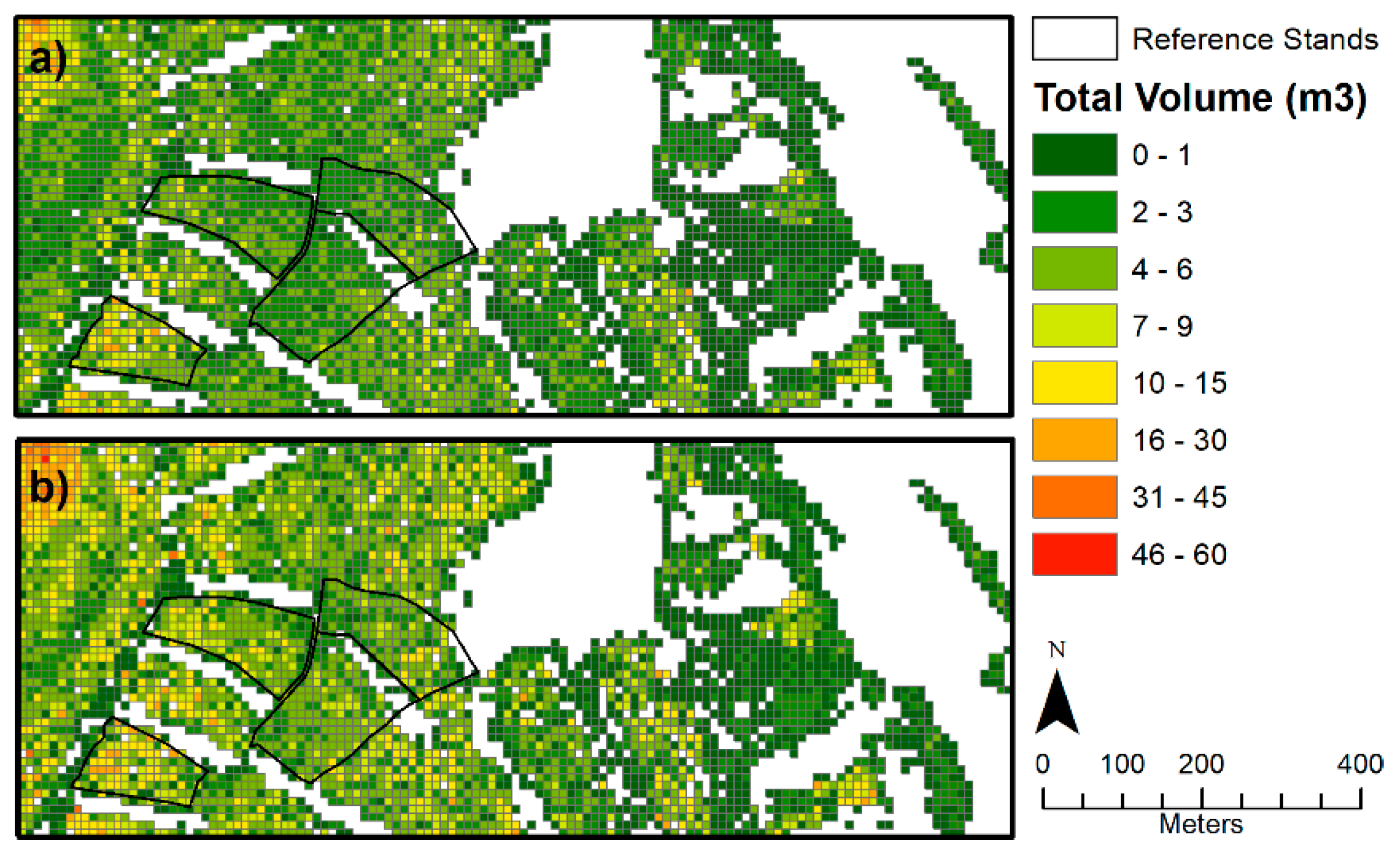
4.3. Total Volume
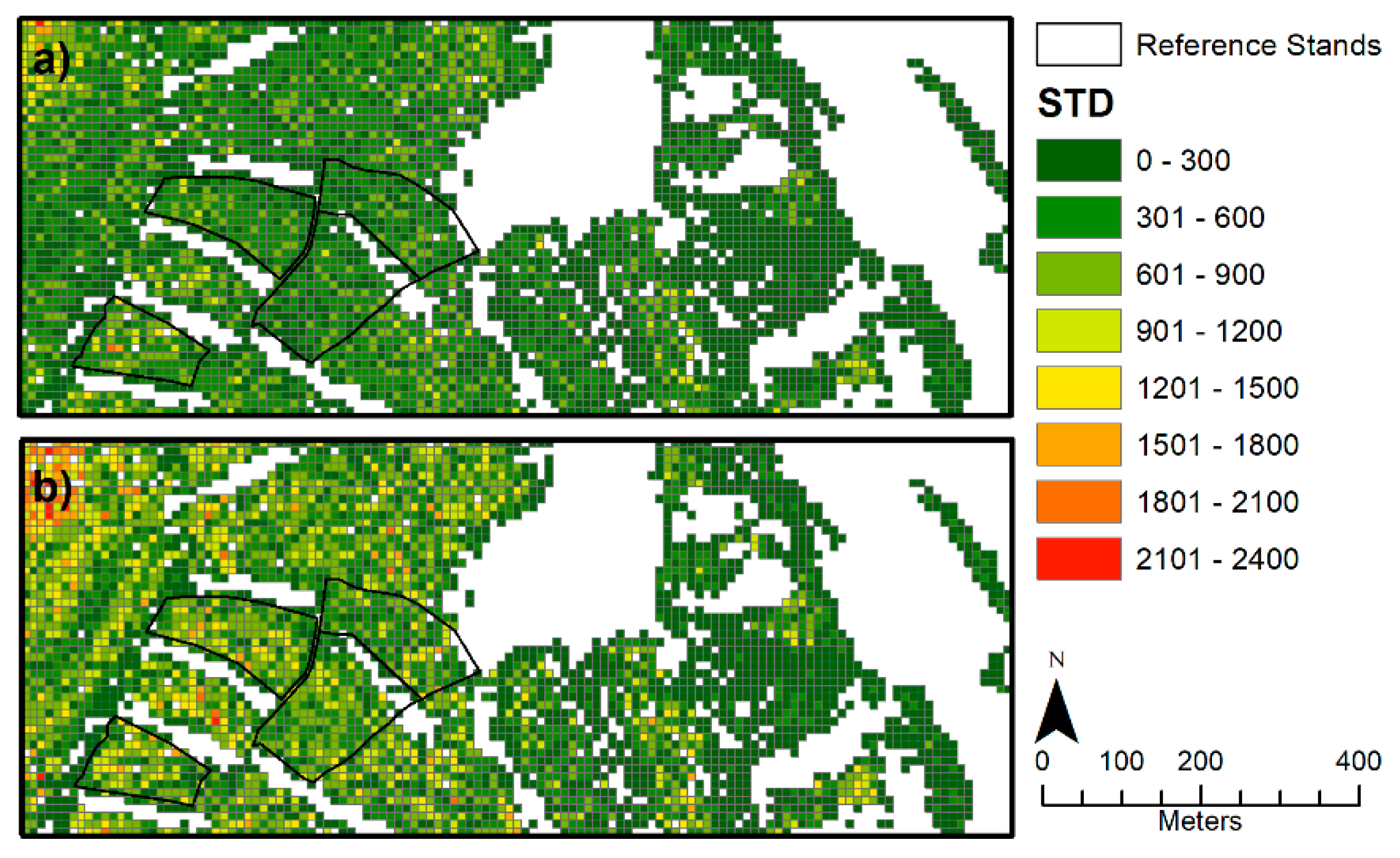
4.4. Stand Density Index
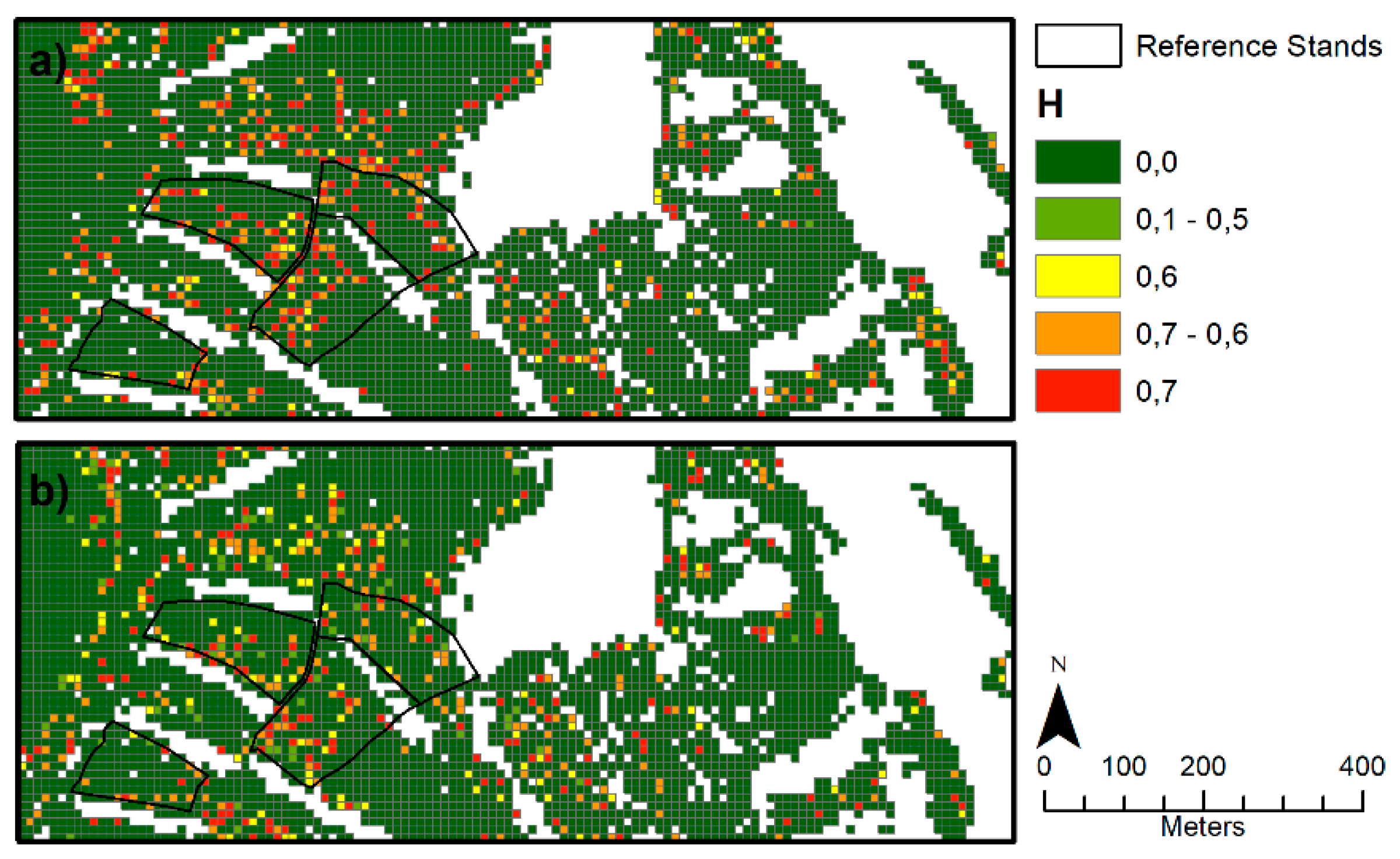
4.5. Shannon’s Diversity Index
5. Conclusions
Author Contributions
Funding
Acknowledgments
Conflicts of Interest
Abbreviations
| GNSS | Global Navigation Satellite System |
| IUFRO | International Union of Forest Research Organizations |
| FAO | Food and Agriculture Organization of the United Nations References |
| ESRI shp | Environmental Systems Research Institute Shapefile |
References
- Véga, C.; Renaud, J.; Durrieu, S.; Bouvier, M. On the interest of penetration depth, canopy area and volume metrics to improve Lidar-based models of forest parameters. Remote Sens. Environ. 2016, 175, 32–42. [Google Scholar] [CrossRef]
- Zhang, Z.; Cao, L.; She, G. Estimating Forest Structural Parameters Using Canopy Metrics Derived from Airborne LiDAR Data in Subtropical Forests. Remote Sens. 2017, 9, 940. [Google Scholar] [CrossRef]
- Vauhkonen, J.; Maltamo, M.; McRoberts, R.E.; Næsset, E. Introduction to forestry applications of airborne laser scanning. In Forestry Application of Airborne Laser Scanning: Concept and Case Studies; Maltamo, M., Næsset, E., Vauhkonen, J., Eds.; Springer Netherlands: Dordrecht, The Netherlands, 2014; pp. 1–16. [Google Scholar]
- Tuominen, S.; Pitkänen, J.; Balazs, A.; Korhonen, K.T.; Hyvönen, P.; Muinonen, E. NFI plots as complementary reference data in forest inventory based on airborne laser scanning and aerial photography in Finland. Silva Fenn. 2014, 48. [Google Scholar] [CrossRef] [Green Version]
- Zhen, Z.; Quackenbush, L.J.; Zhang, L. Trends in Automatic Individual Tree Crown Detection and Delineation—Evolution of LiDAR Data. Remote Sens. 2016, 8, 333. [Google Scholar] [CrossRef]
- Lee, A.C.; Lucas, R.M. A LiDAR-derived canopy density model for tree stem and crown mapping in Australian forests. Remote Sens. Environ. 2007, 111, 493–518. [Google Scholar] [CrossRef]
- Morsdorf, F.; Meiera, E.; Kötza, B.; Ittena, K.I.; Dobbertinc, M.; Allgöwer, B. LiDAR-based geometric reconstruction of boreal type forest stands at single tree level for forest and wildland fire management. Remote Sens. Environ. 2004, 92, 353–362. [Google Scholar] [CrossRef]
- Gupta, S.; Weinacker, H.; Koch, B. Comparative analysis of clustering-based approaches for 3-D single tree detection using airborne fullwave LiDAR data. Remote Sens. 2010, 2, 968–989. [Google Scholar] [CrossRef]
- Li, W.; Guo, Q.; Jakubowski, M.K.; Kelly, M. A new method for segmenting individual trees from the LiDAR point cloud. Photogramm. Eng. Remote Sens. 2012, 78, 75–84. [Google Scholar]
- Popescu, S.C.; Zhao, K. A voxel-based LiDAR method for estimating crown base height for deciduous and pine trees. Remote Sens. Environ. 2008, 112, 767–781. [Google Scholar] [CrossRef]
- Wu, B.; Yu, B.; Yue, W.; Shu, S.; Tan, W.; Hu, C.; Huang, Y.; Wu, J.; Liu, H. A voxel-based method for automated identification and morphological parameters estimation of individual street trees from mobile laser scanning data. Remote Sens. 2013, 5, 581–611. [Google Scholar] [CrossRef]
- Amiria, N.; Polewskic, P.; Heurich, M.; Krzystek, P.; Skidmore, A.K. Adaptive stopping criterion for top-down segmentation of ALS point clouds in temperate coniferous forests. ISPRS J. Photogramm. Remote Sens. 2018, 141, 265–274. [Google Scholar]
- Reitberger, J.; Schnörr, C.; Krzystek, P.; Stilla, U. 3D Segmentation of single trees exploiting full waveform LiDAR data. ISPRS J. Photogramm. Remote Sens. 2009, 64, 561–574. [Google Scholar]
- Tiede, D.; Hoffmann, C. Process oriented object-based algorithms for single tree detection using laser scanning data. In Proceedings of the Workshop on 3D Remote Sensing in Forestry, Vienna, Austria, 14–15 February 2006; p. 5. [Google Scholar]
- Ene, L.; Næsset, E.; Gobakken, T. Single tree in heterogeneous boreal forests using airborne laser scanning and area-based stem number estimates. Int. J. Remote Sens. 2012, 33, 5171–5193. [Google Scholar] [CrossRef]
- Swetnam, T.L.; Falk, D.A. Application of metabolic scaling theory to reduce error in local maxima tree segmentation from aerial LiDAR. For. Ecol. Manag. 2014, 323, 158–167. [Google Scholar] [CrossRef]
- Salas, C.; Ene, L.; Gregoire, T.G.; Næsset, E.; Gobakken, T. Modelling tree diameter from airborne laser scanning derived variables: A comparison of spatial statistics models. Remote Sens. Environ. 2010, 114, 1277–1285. [Google Scholar] [CrossRef]
- Packalén, P.; Maltamo, M. The estimation of species-specific diameter distribution using airborne laser scanning and aerial photographs. Can. J. For. Res. 2008, 38, 1750–1760. [Google Scholar] [CrossRef]
- Flewelling, J.W. Probability models for individually segmented tree crown images in a sampling context. In Proceedings of the SilviLaser 2008 8th International Conference on LiDAR Applications in Forest Assessment and Inventory, Heriot-Watt University, Edinburgh, UK, 17–19 September 2008; pp. 284–294. [Google Scholar]
- Breidenbach, J.; Næsset, E.; Lien, V.; Gobakken, T.; Solberg, S. Prediction of species specific forest inventory attributes using a nonparametric semi-individual tree crown approach based on fused airborne laser scanning and multispectral data. Remote Sens. Environ. 2010, 114, 911–924. [Google Scholar] [CrossRef]
- Lahivaara, T.; Seppanen, A.; Kaipio, J.P.; Vauhkonen, J.; Korhonen, L.; Tokola, T.; Maltamo, M. Bayesian approach to tree detection based on airborne laser scanning data. IEEE Trans. Geosci. Remote Sens. 2014, 52, 2690–2699. [Google Scholar] [CrossRef]
- Melville, G.; Stone, C.; Turner, R. Application of LiDAR data to maximise the efficiency of inventory plots in softwood plantations. N. Z. J. For. Sci. 2015, 45, 16. [Google Scholar] [CrossRef]
- Kansanen, K.; Vauhkonen, J.; Lahivaara, T.; Mehtatalo, L. Stand density estimators based on individual tree detection and stochastic geometry. Can. J. For. Res. 2016, 46, 1359–1366. [Google Scholar] [CrossRef] [Green Version]
- Eysn, L.; Hollaus, M.; Lindberg, E.; Berger, F.; Monnet, J.M.; Dalponte, M.; Kobal, M.; Pellegrini, M.; Lingua, E.; Mongus, D.; Pfeifer, N. A benchmark of LiDAR-based single tree detection methods using heterogeneous forest data from the Alpine space. Forests 2015, 6, 1721–1747. [Google Scholar] [CrossRef]
- Petráš, R.; Pajtík, J. Sustava cesko-slovenskych objemovych tabuliek drevin. Lesnicky casopis. 1991, 37, 49–56. (In Slovak) [Google Scholar]
- Sackov, I.; Hlásny, T.; Bucha, T.; Juriš, M. Integration of tree allometry rules to treetops detection and tree crowns delineation using airborne lidar data. IForest 2017, 10, 459–467. [Google Scholar] [CrossRef]
- Smreček, R.; Michnová, Z.; Sačkov, I.; Danihelová, Z.; Levická, M.; Tuček, J. Determining basic forest stand characteristics using airborne laser scanning in mixed forest stands of Central Europe. IForest 2018, 11, 181–188. [Google Scholar] [CrossRef] [Green Version]
- OPALS Manual. Orientation and processing of airborne laser scanning data: User documentation. Available online: http://geo. tuwien.ac.at/opals/html/index.html (accessed on 5 November 2018).
- Šmelko, Š.; Šebeň, V.; Bošeľa, M.; Sačkov, I.; Kulla, L. New Variants of Methods for Multi-Purpose Inventory and Monitoring of Forest Ecosystems Using Progressive Technologies; NLC-LVÚ Zvolen: Zvolen, Slovakia, 2014; p. 368. ISBN 978-80-8093-193-3. (In Slovak) [Google Scholar]
- Akkay, A.E.; Oguz, H.; Karas, I.R.; Aruga, K. Using LiDAR technology in forestry activities. Environ. Monit. Assess. 2009, 151, 117–125. [Google Scholar] [CrossRef] [PubMed]
- Næsset, E. Predicting forest stand characteristics with airborne scanning laser using a practical two-stage procedure and field data. Remote Sens. Environ. 2002, 80, 88–99. [Google Scholar] [CrossRef]
- Andersen, H.E.; Reutebuch, S.E.; McGaughey, R.J. A rigorous assessment of tree height measurements obtained using airborne lidar and conventional field methods. Can. J. Remote Sens. 2006, 32, 355–366. [Google Scholar] [CrossRef]
- Takahashi, T.; Yamamoto, K.; Senda, Y.; Tsuzuku, M. Estimating individual-tree heights of sugi (Cryptomeria japonica D. Don) plantations in mountainous areas using small-footprint airborne LiDAR. J. For. Res. 2005, 10, 135–142. [Google Scholar] [CrossRef]
- Kaartinen, H.; Hyyppä, J. Tree extraction-Report of EuroSDR project. Available online: https://www.google.com.hk/url?sa=t&rct=j&q=&esrc=s&source=web&cd=1&ved=2ahUKEwi-hPOa6MfiAhXMyYsBHaRMD80QFjAAegQIAxAC&url=http%3A%2F%2Fbono.hostireland.com%2F~eurosdr%2Fpublications%2F53.pdf&usg=AOvVaw3iEPzkFdw06CbOp6niCnOx (accessed on 5 November 2018).
- Yu, X.; Hyyppä, J.; Vastaranta, M.; Holopainen, M. Predicting individual tree attributes from airborne laser point clouds based on random forest technique. ISPRS J. Photogramm. Remote Sens. 2011, 66, 28–37. [Google Scholar]
- Wu, J.; Yao, W.; Choi, S.; Park, T.; Myneni, R.B. A comparative study of predicting DBH and stem volume of individual trees in a temperate forest using airborne waveform LiDAR. IEEE Geosci. Remote Sens. Lett. 2015, 12, 2267–2271. [Google Scholar] [CrossRef]
- Kandare, K.; Dalponte, M.; Ørka, H.O.; Frizzeria, L.; Næsset, E. Prediction of Species-Specific Volume Using Different Inventory Approaches by Fusing Airborne Laser Scanning and Hyperspectral Data. Remote Sens. 2017, 9, 400. [Google Scholar] [CrossRef]
- Peuhkurinen, J.; Mehtätalo, L.; Maltamo, M. Comparing individual tree detection and the area-based statistical approach for the retrieval of forest stand characteristics using airborne laser scanning in Scots pine stands. Can. J. For. Res. 2011, 41, 583–598. [Google Scholar] [CrossRef]
- Næsset, E. Practical large-scale forest stand inventory using a small-footprint airborne scanning laser. Scand. J. For. Res. 2004, 19, 164–179. [Google Scholar]
- Tesfamichael, S.G.; Aardt, J.A.N.; Ahmed, F. Estimating plot-level tree height and volume of Eucalyptus grandis plantations using small-footprint, discrete return LiDAR data. Prog. Phys. Geogr. 2010, 34, 515–540. [Google Scholar] [CrossRef]
- Moore, M.M.; Deiter, D.A. Stand Density Index as a Predictor of Forage Production in Northern Arizona Pine Forests. J. Range Manag. 1992, 45, 267–271. [Google Scholar] [CrossRef]
- Vauhkonen, J.; Ene, L.; Gupta, S.; Heinzel, J.; Holmgren, J.; Pitkänen, J.; Solberg, S.; Wang, Y.; Weinacker, H.; Hauglin, K.M.; Lien, V.; Packalén, P.; Gobakken, T.; Koch, B.; Næsset, E.; Tokola, T.; Maltamo, M. Comparative testing of single-tree detection algorithms under different types of forest. Forestry 2012, 85, 27–40. [Google Scholar] [CrossRef]
- Yu, X.; Hyyppä, J.; Litkey, P.; Kaartinen, H.; Vastaranta, M.; Holopainen, M. Single-Sensor Solution to Tree Species Classification Using Multispectral Airborne Laser Scanning. Remote Sens. 2017, 9, 108. [Google Scholar] [CrossRef]
- Ballanti, L.; Blesius, L.; Hines, E.; Kruse, B. Tree Species Classification Using Hyperspectral Imagery: A Comparison of Two Classifiers. Remote Sens. 2016, 8, 445. [Google Scholar] [CrossRef]
- Ørka, H.O.; Næsset, E.; Bollandsås, O.M. Classifying species of individual trees by intensity and structure features derived from airborne laser scanner data. Remote Sens. Environ. 2009, 113, 1163–1174. [Google Scholar] [CrossRef]
- Korpela, I.; Ørka, H.O.; Maltamo, M.; Tokola, T. Tree species classification using airborne LiDAR-effects of stand and tree parameters, downsizing of training set, intensity normalization and sensor type. Silva Fenn. 2010, 44, 319–339. [Google Scholar] [CrossRef]
- Dalponte, M.; Ene, L.T.; Gobakken, T.; Næsset, E.; Gianelle, D. Predicting Selected Forest Stand Characteristics with Multispectral ALS Data. Remote Sens. 2018, 10, 586. [Google Scholar] [CrossRef]


| Stand | SR (%) | A (ha) | S (°) | NPH | hdq (m) | dq (cm) | VPH (m3) | SDI | H |
|---|---|---|---|---|---|---|---|---|---|
| C | ≥70 | 1.64 | 16.52 | 241 | 33.70 | 43.01 | 520.77 | 575.4 | 0.69 |
| CB | ≈ 60/40 | 1.90 | 5.62 | 199 | 27.31 | 35.76 | 229.89 | 353.3 | 0.64 |
| BC | ≈ 60/40 | 2.70 | 4.56 | 366 | 24.59 | 30.69 | 292.95 | 508.1 | 0.60 |
| B | ≥\70 | 1.85 | 10.72 | 364 | 25.20 | 31.73 | 337.97 | 533.4 | 0.55 |
| Tree Species Group | Model Forms | N | R | R2 | SEE | SEE% | p-Level |
|---|---|---|---|---|---|---|---|
| Broadleaves | DBH = 6.152 × exp(0.058 × h) + ε | 769 | 0.85 | 0.72 | 6.2 | 18.9 | <0.001 |
| Conifers | DBH = 8.054 × exp(0.053 × h) + ε | 603 | 0.88 | 0.78 | 7.3 | 19.1 | <0.001 |
| Reference Stands | Multi.-Based Method | Raster-Based Method | ||||||
|---|---|---|---|---|---|---|---|---|
| ER | MR | CR | OR | ER | MR | CR | OR | |
| C | 67 | 58 | 9 | 42 | 97 | 64 | 33 | 36 |
| CB | 65 | 57 | 8 | 43 | 96 | 56 | 40 | 44 |
| BC | 64 | 56 | 8 | 44 | 92 | 58 | 34 | 42 |
| B | 66 | 55 | 11 | 45 | 89 | 52 | 37 | 48 |
| Average | 66 | 57 | 9 | 44 | 94 | 58 | 36 | 43 |
| Stand and Ecological Variables | C | CB | BC | B | All | ||
|---|---|---|---|---|---|---|---|
| ei% | e% | se% | RMSE% | ||||
| Mean height | −4.3 | 1.2 | 9.1 | 9.2 | 3.1 | 6.5 | 7.2 |
| Mean diameter | 6.7 | −0.6 | 10.9 | 11.8 | 6.9 | 5.7 | 8.6 |
| Total volume | −10.2 | −11.7 | −21.3 | −14.9 | −14.2 | 4.9 | 15.0 |
| Stand density index | −30.3 | −24.3 | −33.1 | −24.8 | −28.3 | 4.3 | 29.0 |
| Shannon’s diversity index | −1.2 | 3.9 | 7.8 | −10.1 | 0.4 | 7.7 | 7.2 |
| Stand and Ecological Variables | C | CB | BC | B | All | ||
|---|---|---|---|---|---|---|---|
| ei% | e% | se% | RMSE% | ||||
| Mean height | −2.8 | 0.1 | 7.3 | 8.9 | 2.8 | 5.6 | 6.1 |
| Mean diameter | 7.7 | −2.2 | 8.1 | 11.2 | 6.1 | 5.8 | 8.3 |
| Total volume | 3.8 | 29.3 | 19.1 | 30.6 | 18.7 | 12.4 | 21.4 |
| Stand density index | −15.0 | 5.3 | 4.4 | 17.5 | 2.5 | 13.5 | 14.7 |
| Shannon’s diversity index | −4.8 | 1.7 | 1.1 | −8.6 | −2.5 | 5.0 | 5.3 |
| Method | Height (m) | Diameter (cm) | Volume (m3) | SDI | H | |||||
|---|---|---|---|---|---|---|---|---|---|---|
| Mean | SD | Mean | SD | Mean | SD | Mean | SD | Mean | SD | |
| Multi-based | 25.7 | 8.9 | 34.1 | 13.2 | 2.9 | 2.6 | 366.6 | 246.6 | 0.7 | 0.2 |
| Raster-based | 24.6 | 9.9 | 32.6 | 14.5 | 4.1 | 4.3 | 518.3 | 416.6 | 0.6 | 0.2 |
© 2019 by the authors. Licensee MDPI, Basel, Switzerland. This article is an open access article distributed under the terms and conditions of the Creative Commons Attribution (CC BY) license (http://creativecommons.org/licenses/by/4.0/).
Share and Cite
Sačkov, I.; Kulla, L.; Bucha, T. A Comparison of Two Tree Detection Methods for Estimation of Forest Stand and Ecological Variables from Airborne LiDAR Data in Central European Forests. Remote Sens. 2019, 11, 1431. https://doi.org/10.3390/rs11121431
Sačkov I, Kulla L, Bucha T. A Comparison of Two Tree Detection Methods for Estimation of Forest Stand and Ecological Variables from Airborne LiDAR Data in Central European Forests. Remote Sensing. 2019; 11(12):1431. https://doi.org/10.3390/rs11121431
Chicago/Turabian StyleSačkov, Ivan, Ladislav Kulla, and Tomáš Bucha. 2019. "A Comparison of Two Tree Detection Methods for Estimation of Forest Stand and Ecological Variables from Airborne LiDAR Data in Central European Forests" Remote Sensing 11, no. 12: 1431. https://doi.org/10.3390/rs11121431