Article

Continuous Monitoring of the Spatio-Temporal Patterns of Surface Water in Response to Land Use and Land Cover Types in a Mediterranean Lagoon Complex

1
Ministry of Education Key Laboratory for Earth System Modeling, Department of Earth System Science, Tsinghua University, Beijing 100084, China
2
Computer Science and Technology, Harbin Institute of Technology, WeiHai 264200, China
3
ESPACE-DEV, UMR 228 IRD/UM/UR/UG, Institut de Recherche pour le Développement (IRD), 500 rue Jean-François Breton, 34093 Montpellier, France
4
Department of Geography, University of Brasilia, Brasilia 70910-900, Brazil
5
Joint Center for Global Change Studies, Beijing 100084, China
*
Author to whom correspondence should be addressed.
Remote Sens. 2019, 11(12), 1425; https://doi.org/10.3390/rs11121425
Submission received: 8 May 2019 / Revised: 1 June 2019 / Accepted: 7 June 2019 / Published: 15 June 2019
(This article belongs to the Section Environmental Remote Sensing)

Abstract

:
Mediterranean coastal lagoons and their peripheral areas often provide a collection of habitats for many species, and they often face significant threats from anthropogenic activities. Diverse human activities in such areas directly affect the spatio-temporal dynamic of surface water and its ecological characteristics. Monitoring the surface water dynamic, and understanding the impact of human activities are of great significance for coastal lagoon conservation. The Regional Natural Park of Narbonne includes a typical Mediterranean lagoon complex where surface water dynamic and its potential link with local diverse human activities has not yet been studied. In this context, based on all the available Landsat images covering the study area during 2002–2016, this study identified the water and non-water classes for each satellite observation by comparing three widely used spectral indices (i.e., NDVI, NDWI and MNDWI) and using the Otsu method. The yearly water frequency index was then computed to present the spatio-temporal dynamic of surface water for each year, and three water dynamic scenarios were also identified for each year: permanent water (PW), non-permanent water (NPW) and non-water (NW). The spatial and inter-annual variation in the patterns of the three water scenarios were characterized by computing the landscape metrics at scenario-level quantifying area/edge, shape, aggregation and fragmentation. Finally, the quantitative link between different land use and land cover (LULC) types derived from the LULC maps of 2003, 2012 and 2015 and the surface water dynamic scenarios was established in each of the 300 m × 300 m grid cells covering the study area to determine the potential impact of human activities on the surface water dynamic. In terms of the inter-annual variation during 2002–2016, PW presented an overall stability, and NPW occupied only a small part of the water surface in each year and presented an inter-annual fluctuation. NPW had a smaller patch size, with lower connectivity degree and higher fragmentation degree. In terms of spatial variation during 2002–2016, NPW often occurred around PW, and its configurational features varied from place to place. Moreover, PW mostly corresponded to the natural lagoon, and salt marsh (as a part of lagoons), and NPW had a strong link with arable land (agricultural irrigation) and salt marsh (salt production), sand beach/dune, coastal wetlands and lagoon for the LULC maps of 2003, 2012 and 2015. However, more in-depth analysis is required for understanding the impact of sand beach/dune, coastal wetlands and lagoon on surface water dynamics. This study covers the long-term variations of surface water patterns in a Mediterranean lagoon complex having intense and diverse human activities, and the potential link between LULC types and the water dynamic scenarios was investigated on different dates. The results of the study should be useful for environmental management and protection of coastal lagoons.

Graphical Abstract

1. Introduction

Coastal lagoons are particular ecosystems located in the transitional areas between land and sea, and occur along nearly 15% of the global shorelines worldwide [1]. More than 100 coastal lagoons are located in the Mediterranean and these provide a variety of habitats for many species and support various human activities, such as agriculture, tourism, and mining [2,3]. These land uses or coverage patterns often have a relevant impact on the hydrology of special coastal systems in coastal areas such as lagoons and estuaries, with a strong impact on water storage and drainage rate [4,5]. The high human density in Mediterranean coastal areas and the strong dependence of regional economic development on a lagoon complex often means such areas are very vulnerable [6,7].
Over the past years, social awareness in protection and management of Mediterranean coastal lagoons has been increasing [2]. Many Mediterranean coastal lagoons have been included in lagoon management programs, such as the Ramsar convention, an international treaty that recognizes the international importance of wetlands, and urges its member states to maintain the ecological characteristics of wetlands and develop a sustainable-use plan through local, regional, national and international cooperation [8]. Natura 2000, the European project of biodiversity preservation, aims to ensure the long-term survival of species and habitats protected under the Birds and Habitats Directive [9]. More specifically, Natura 2000 has developed an approach for evaluating the conservation status of lagoon complexes. These have been implemented at the scale of water patch, and the necessary data for the evaluation (e.g., surface, sediment, macrophyte, etc.,) are also collected at such a scale [10]. Therefore, extracting surface water, monitoring the spatio-temporal dynamic of surface water, and compositional and configurational features of water patches and studying their association with different land use and land cover (LULC) types are important for the management and protection of coastal lagoon complexes.
Optical images like MODIS (Moderate Resolution Imaging Spectroradiometer) have been widely used in studies at a global or regional scale and over a long time span [11,12,13,14]. Their coarse spatial resolution is a great limitation for small water patches, particularly in a coastal lagoon complex. Images with high spatial resolution have been applied in such studies to provide more detailed spatial information of water bodies [15,16,17]. However, they cannot cope with frequent, or even continuous observation at a relatively large spatial scale [18]. Landsat images are the compromise solution with a 30 m spatial resolution and a 16 day revisit time, and have the longest record permitting open water monitoring from the 1970s [19]. With the development of remote sensing technology, Sentinel-2 data, with a great revisit frequency and a higher spatial resolution than Landsat data [20], have been gradually introduced for water mapping in recent years [21,22]. Nevertheless, Sentinel-2 images are not able to provide water monitoring data before 2015. A systematic review proposed by Guo et al. (2017) [23] confirmed that Landsat TM/ETM+/OLI data were the most used remote sensing data in wetland mapping. Therefore, taking account of the spatial and temporal resolution of these remote sensing data, Landsat images are particularly suitable for frequent identification of the surface water and studying the timing and frequency of ephemeral water patches, while using all available Landsat images [24,25].
Multi-spectral indices and thresholding methods are widely used to extract surface water bodies from optical remote sensing images as they are quite fast and simple, especially for large-scale and/or long-term time series studies [24,26,27,28]. Many water spectral indices, such as the Automated Water Extraction Index (AWEI) [29], Normalized Difference Water Index (NDWI) [30], Modified Normalized Difference Water Index (MNDWI) [31], Tasseled Cap Wetness Index (TCW) [32,33], and Water Index (WI) [34], were developed for identifying surface water. Moreover, vegetation spectral indices, such as the Normalized Difference Vegetation Index (NDVI), were originally developed for vegetation detection [35], but have also been used to extract water features [36,37]. Of these, some studies applied only the empirically optimal threshold value directly, such as the zero of MNDWI [24] and others compared two or more indices according to the classification accuracy and/or their spatial performance [38]. However, standard threshold values of a single index do not lead to good accuracy [39] and, depending on the area, it is difficult to identify location, weather, and time of acquisition [15,36,40], especially in a lagoon complex with challenging conditions for surface water detection, such as varying salinity, turbidity, depth, and/or eutrophication. Thus, for monitoring the frequency and accuracy of surface water over a long period of time, it is necessary to select the optimal indices, and determine the real time optimal threshold. As one of successful thresholding algorithms, Otsu’s method [41] was conventionally used in previous studies for automatically give the real time threshold values [21,42,43,44].
Considering the spatio-temporal dynamic of surface water, an effective technique is the water frequency index (WFI), which can reflect the intra-annual and inter-annual variations of surface water and their spatial distribution at pixel level, and also permits to identify different types of surface water dynamic by dividing index values into different value intervals, such as permanent water (PW), non-permanent water (NPW) and non-water (NW) [26,27,28,45,46]. Besides, landscape metrics are widely applied to analyze the compositional and configurational features of the LULC types in a landscape, particularly in the framework of wetlands characterization [47,48]. The measurement and analysis of the degree of the spatial overlap (i.e., co-occurrence) of LULC types and water dynamic types might be one approach for understanding the potential link between water dynamic and LULC typologies during a given period. In fact, spatial co-occurrence statistics are typical methods that were widely used in ecological studies for quantifying the spatial pattern of the co-occurrence of target ecological variables (i.e., different species or underlying environmental factors and species) for explaining their ecological links [49,50,51,52]. A quite straight-forward method is the summarizing of the number of checkerboard units having the similar co-occurrence patterns [49,51].
This paper concerns the littoral part of the Regional Natural Park of Narbonne, a typical Mediterranean lagoon complex. This lagoon complex was also recognized in 2006 as a “wetland of international importance” under the Ramsar Convention, and 56% of the territory of the park is registered in the Natura 2000 network [53]. It contains, on the one hand, habitats of priority interest, whereby France has an obligation to preserve or restore to good condition and, on the other hand, it has to face the pressures of riparian anthropogenic dynamics. Water patches often act as critical refuges and breeding areas, offer food sources for wildlife, and harbor many plant and animal species that would otherwise not survive in the surrounding landscape. Clearly, it is very important to monitor the surface water dynamics for water management, ecosystem assessment and biodiversity conservation over the long term. However, the long-term spatio-temporal dynamic of surface water patches of this area has yet to be studied. Moreover, the association between the surface water dynamic and LULC types has also not been well-studied yet.
In this context, this study aims to give an overall retrospect of the surface water dynamic of the lagoon complex in the Regional Natural Park of Narbonne, and to diagnose the influence of anthropologic activities on water dynamic frequency during 2002–2016, including:
  • Comparing spectral indices and monitoring yearly surface water frequency maps using all available Landsat images during the entire study period;
  • Analyzing the spatio-temporal variations of the compositional and configurational patterns of water patches using landscape metrics;
  • Studying the relationship between yearly surface water dynamics and different LULC types based on the existing multi-date LULC maps.
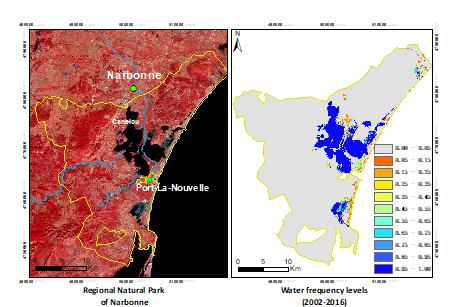
2. Study Area

This study was carried out in the Regional Natural Park of Narbonne (RNPN) that is located on the coast of the department of Aude in the Languedoc-Roussillon region, France (Figure 1). The lagoon complex extends 14 km from north to south, from Narbonne to Port-la-Nouvelle, and 10 km from west to east, from Peyriac-de-Mer to the Mediterranean Sea. The water bodies in this area consist of four lagoons (i.e., Bages-Sigean, Ayrolle, Campignol, and Gruissan), three canals (i.e., La Robine, La Berre and Rieu de Roquefort) and some water areas surrounding the lagoons.
The Bages-Sigean lagoon (3700 hectares) is divided into several sectors which connect to each other (i.e., the northern, middle and southern sector of Bages-Sigean, abbreviated as BGN, BGM and BGS, respectively) and also connect to the Mediterranean Sea at Port-la-Nouvelle. This lagoon is almost permanently fed with freshwater mainly from the canal of La Berre and the canal of La Robine via the Canelou River. The canal of La Robine passes through a large agricultural zone in the low plain in the northern part, then joins the Bages-Sigean lagoon passing by the Île-Saint-Lucia island, and ends its journey in the sea at Port-la-Nouvelle. Water is extracted from the canals to the land to decrease soil salinity in the vine plots on the low plain and also for the irrigation of annual crops and impoundment of rice fields. The Campignol lagoon (115 hectares) is located between the low plain in the north and the Ayrolle lagoon (1320 hectares) in the south. The two lagoons are connected through a narrow channel. The Gruissan lagoon (145 hectares) is situated between the massif of La Clappe and the village of Gruissan and joins the sea by the canal of Grazel. From the second half of the twentieth century, human activity (e.g., fishing, shellfish farming, tourism, navigation, etc.) and the growth of the population began to lead to a significant increase in pollution and nutrients in these lagoons, which triggered the phenomenon of eutrophication.
This area has a typical Mediterranean climate of long, hot and dry summers, and mild and humid winters, with approximately 300 days of sunshine per year. This means that observation from optical satellites is effective.

3. Data collection and Preprocessing

3.1. Landsat Time Series Images

All available Landsat surface reflectance (SR) data derived from the Landsat 5 Thematic Mapper (TM), Landsat 7 Enhanced Thematic Mapper Plus (ETM+) and Landsat 8 Operational Land Images (OLI) over the period 2002–2016 were downloaded from the United States Geological Survey (USGS) website (http://landsat.usgs.gov/) and were used as the input data for surface water extraction in this study. All Landsat images have been pre-processed to L1TP level (i.e., Standard Terrain Correction) or L1GT level (i.e., Systematic Terrain Correction). Atmospheric correction did not included in such data, which might not be necessary for land cover mapping [54]. Among the 420 images from 2002 to 2016, the number of observations per year varied from 33 in 2002 to 44 in 2016, with minimum observations in 2012 and maximum observations in 2014 (Figure 2a). For each image, a quality assessment (QA) band was applied to replace cloud and cloud shadow with missing values, and the vector layer of the border of RNPN (Figure 1) was then applied to delineate the study area. The remaining pixels within the study area were regarded as serviceable pixels and used for identifying the surface water. Moreover, Figure 2b shows the histogram of the number of missing values in all the Landsat images per year in the study area, and this information ensured the effective and accurate tracking of spatial and inter-annual variations of surface water during 2002–2016. More detailed information of the Landsat spectral bands and spatial resolution is presented in Table 1.

3.2. Validation Data

To evaluate the accuracy of the surface water time series, we chose three different dates (Table 2), which corresponded to three observations derived from Landsat 5 TM, Landsat 7 ETM+ and Landsat 8 OLI, respectively. Meanwhile, they had the close dates with three high spatial resolution images from Google Earth ProTM (Google Inc., Menlo Park, CA, USA). We then randomly generated 600 samples across the study area and visually interpreted them as water and non-water for each date using Google Earth ProTM, and expert’s knowledge. Note that some samples might locate in the missing values caused by the cover of clouds and cloud shadows. The total number of effective samples and the number of samples for water and non-water per date were presented in Table 2.

3.3. Multi-Date Land Use and Land Cover Datasets

To establish the potential link between surface water frequency and LULC types, we used the existing LULC maps of 2003, 2012 and 2015 in vector format covering the study area that were downloaded from the Etalab website (www.data.gouv.fr). These LULC datasets have a hierarchical classification system, with five classes at level 1, fifteen classes at level 2 and forty-one classes at level 3. The maps were realized by visual interpretation based on the orthophotos of 2003, 2012 and 2015. In this study, the LULC types at level 2 were chosen as the reference data, including (class 1) urban built fabric; (class 2) areas of economic activities and transport network; (class 3) areas of material extraction, deposit and waste storage; (class 4) urban green space; (class 5) arable lands; (class 6) vineyard or arboriculture; (class 7) uncultivated lands; (class 8) forest; (class 9) shrubby and herbaceous associations; (class 10) sand beach and sand dune; (class 11) lagoon; (class 12) coastal wetlands; (class 13) salt marsh; (class 14) water flow; (class 15) other water bodies. The map of 2012 was displayed in the right part of Figure 1 for giving a demonstration of the LULC classes.

4. Methodology

4.1. Spectral Index-Based Algorithms for Surface Water Extraction

Among different spectral indices used in surface water extraction in previous studies, we chose NDWI, MNDWI and NDVI that were most commonly used. Initially, NDWI was proposed by Mcfeeters (1996) [30] because it maximizes the surface water reflectance in the green band and minimizes the surface water reflectance in the near infrared band. Based on NDWI, MNDWI was proposed by Xu (2006) [31] to replace the near infrared band with a shortwave infrared band as this is more efficient when identifying open surface water in an urban context.
NDWI = G r e e n N I R G r e e n + N I R
where Green and NIR represent the SR value of the green band and near infrared band, respectively.
MNDWI = G r e e n S W I R 1 G r e e n + S W I R 1
where Green and SWIR1 represent the SR value of the green band and shortwave infrared band, respectively.
NDVI = N I R R e d N I R + R e d
where Red and NIR represent the SR value of the red band and near infrared band, respectively.
Three equations were applied to each Landsat image from the period 2002 to 2016 and the NDWI, MNDWI and NDVI time series were produced. Since the time series Landsat data were acquired at different times and under different weather conditions by different satellite platforms, it would be better to determine the threshold value according to the values of the water index itself [40]. In our study area, the pixel values of water indices often presented a typical bi-modal distribution (Figure 3), we directly applied the Otsu algorithm for each water index. This is a widely-used approach in automatic segmentation of water index values, as it selects the threshold value by maximizing the inter-class variance of surface water and background features [41] and adapts well to an index with a bi-modal distribution [22,43,44].
In addition, based on the 30 m Global Digital Elevation Model (DEM) derived from the Shuttle Radar Topography Mission (SRTM), the solar azimuth and the zenith angle of each image, the terrain shadows were derived, and the pixels misclassified as water, but corresponding to terrain shadows, were removed manually.

4.2. Choice of the Optimal Index for Surface Water Extraction

In order to fully compare the spectral indices used in this study and select the optimal one for further analysis of surface water dynamic, we both qualitatively and quantitatively evaluated the results of the index-based approaches. We first compared the results of water indices with the false color composite (FCC) of the initial Landsat bands in the different areas of interest. The sub-areas were selected to perform comparisons where different patterns of water patch and vegetation disturbance were present. More precisely, the subareas A, B, C and D represent an artificial saltpan, the lagoon estuary with submerged marine vegetation, a small lagoon, and the natural wetlands with irregular borders of surface water, respectively. Their spatial localization was displayed in Figure 1.
Then, to quantitatively evaluate the performance of each index, we used a confusion matrix-based method, by comparing the resulting water and non-water maps with the reference samples in Table 2. The four following parameters were generated (Table 3): (1) true positive (TP): positive instance, positive classified; (2) false positive (FP): negative instance, positive classified; (3) true negative (TN): negative instance, negative classified; and (4) false negative (FN): positive instance, negative classified. Based on these outcomes, we calculated the overall accuracy (OA) and kappa coefficient (kappa) [55] to assess the accuracy of water versus non-water maps derived from the water indices over three different dates.
O A = T P + T N T P + T N + F P + F N ,   k a p p a = T ( T P + T N ) Σ T T Σ
where T is the total number of pixels in the accuracy assessment, and Σ is the chance accuracy that is defined as (TP + FP) * (TP + FN) + (FN + TN) * (FP + TN).

4.3. Analysis of Spatio-Temporal Variations of Surface Water Pattern

4.3.1. Inter-Annual Variation of Surface Water Pattern

To describe the yearly water dynamic over the entire time series (i.e., 2002–2016), a yearly water frequency index (WFI) was computed that was defined as the number of times a pixel is classified as surface water divided by the number of observations without clouds and cloud shadows per pixel position [26,27,28].
W F I = n i j N i j
where n is the number of time the pixels were classified as water, N is the number of observations without clouds and cloud shadows per year, and i, j are the coordinates of pixel.
To further unravel the yearly water dynamic levels and the inter-annual variations of water pixel number at different dynamic levels, we disaggregated the WFI values to 11 intervals (i.e., (0, 0.05], (0.05, 0.15], (0.15, 0.25], (0.25, 0.35], (0.35, 0.45], (0.45, 0.55], (0.55, 0.65], (0.65, 0.75], (0.75, 0.85], (0.85, 0.95], and (0.95, 1]) and the pixel numbers per interval were counted and compared. Then, the WFI layer of each year was post-processed using the following steps for identifying the three water scenarios per year: (1) permanent water (PW) with pixel values greater than 0.75; (2) non-permanent water (NPW) with pixel values greater than 0.05 and less than 0.75; (3) non-water (NW) with pixel values less than 0.05.
To monitor the inter-annual variation of the surface water pattern, a set of landscape metrics, widely used in the analysis of wetland landscapes, was chosen [47,48,56]. The description of a landscape pattern often includes two aspects: (1) composition, relating to the abundance and variety of patch types in the landscape, and (2) configuration, relating to spatial character, arrangement and context of the patches [57]. In this study, the compositional feature was characterized by the percentage (PLAND) of each class in the landscape, and the configurational pattern was characterized by patch density (PD), edge density (ED), area-weighted mean shape index (SHAPE_AM), aggregation index (AI) and landscape division index (DIVISION) (Table 4). Based on the yearly layer of surface water scenarios, the landscape metrics were computed for each of the three surface water scenarios with an 8-connectivity implementation of the algorithm, using Fragstats software 4.2 (Amherst, MA, USA). Here, the study area was considered as the unit of metric computation.

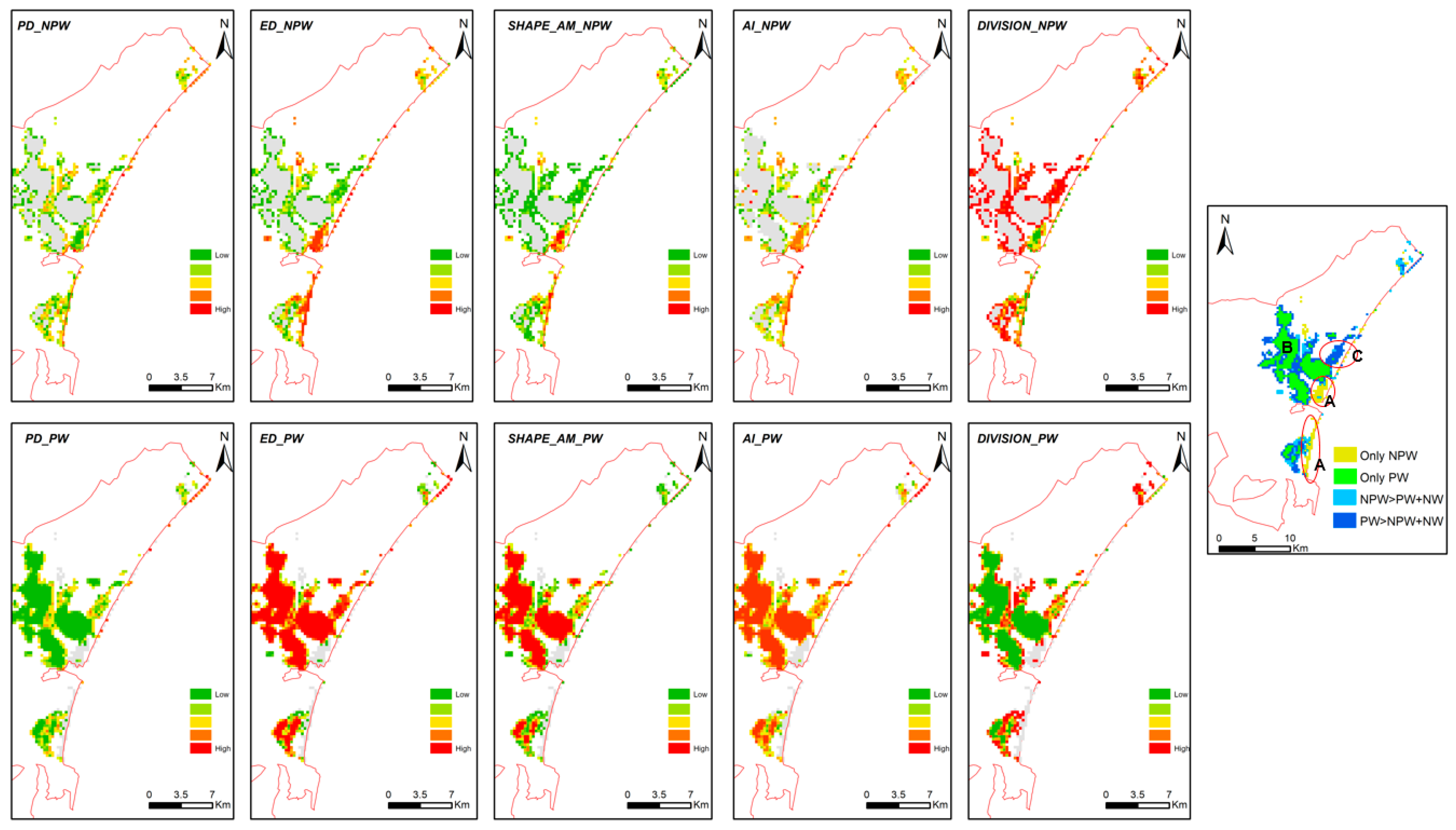
4.3.2. Spatial Variation of Surface Water Pattern

To provide visualization of the spatial variation of surface water during the entire study period (i.e., 2002–2016), a WFI layer of the entire 15 years was produced using Equation (5) and all water versus non-water maps derived from the MNDWI-based method between 2002 and 2016.
Moreover, we divided the study area into regular 300 m × 300 m cells that were used as the units of spatial analysis. Based on the layers of yearly surface water scenarios, the configuration metrics in Table 4 were then computed at scenario-level in each cell for each of the 15 years, and the average value of landscape metrics per cell for the entire study period was computed to spatially compare the variation of the patterns of PW and NPW patches.

4.4. Implications of Land Use and Land Cover to Surface Water Dynamic

To investigate the potential link between the surface water dynamic scenarios and LULC over the entire time series, we used the multi-date LULC datasets (i.e., LULC maps of 2003, 2012 and 2015), and analyzed the degree of the spatial overlap between LULC types and water dynamic scenarios at a scale of 300 m × 300 m for 2003, 2012 and 2015. First, we recalculated the new WFI layers for 2003, 2012 and 2015, using all the water versus non-water maps in the intervals of 2002–2004, 2011–2013 and 2014–2016, respectively, and the three water scenarios (i.e., PW, NPW and NW) in 2003, 2012 and 2015 were identified. Based on the vector grid layer of 300 m × 300 m cell size, the cells having the majority value of PW, NPW or NW were labeled as cell of PW, cell of NPW or cell of NW, respectively. Meanwhile, the same procedure was carried out for labelling each of the cells by comparing the frequency of occurrence of LULC types per cell. Finally, each cell was assigned two attributes (i.e., the majority value of one water dynamic class and the majority value of one LULC type), and the number of cells having the same attributes (e.g., NPW versus salt marsh) were counted to display the quantitative matchup between water dynamic scenarios and different LULC types.
Moreover, according to LULC types in the multi-dates LULC datasets, the average value of WFI of the NPW class per LULC class was computed and compared for 2002–2004, 2011–2013 and 2014–2016, to determine the impact intensity of different LULC types on water occurrence frequency.

5. Results

5.1. Choice of the Optimal Index Based on Qualitative and Quantitative Evaluation for Surface Water Extraction

Figure 4 presents a visual comparison between an index-based surface water map and an FCC map. In the case of sub-area, A, it shows that MNDWI performed better than the other indices when identifying fine regular borders located in the surface water of an artificial saltpan. In the case of sub-area B, it presents the submerged marine vegetation in the estuary of the lagoon where the water depth is often very shallow and submerged vegetation often emerges at the water surface. Except for MNDWI, the remaining indices did not seem to correctly identify the surface water, while some water pixels were misclassified as non-water pixels due to the disturbance of submerged marine vegetation. In the case of sub-area C, apart from NDVI, the two other indices appear to detect surface water well, and there is not great difference in the results. The grey blocks present the missing data caused by clouds and cloud shadows. In the case of sub-area D, MNDWI adapted better in identifying the irregular borders of surface water in the natural wetlands. Therefore, based on the visual comparison, MNDWI appears more appropriate for detecting surface water and is therefore more suitable for characterizing landscape patterns by computing the landscape metrics.
Since the surface water maps were derived from three spectral indices during 2002–2016, we implemented a quantitative evaluation on three dates that corresponded to the different Landsat satellite platforms (Landsat TM, Landsat ETM+ and Landsat OLI). We also assumed that the classification accuracy of index maps with the same platform were similar. The surface water map derived from the different indices all had high accuracies with an OA of 95%–98% and high Kappa coefficients of 0.85–0.94 (Table 5). MNDWI had a high value of OA and Kappa in both the evaluation of 2008 and 2016.
Based on the results of both visual inspection and quantitative evaluation, MNDWI was finally selected as the optimal index for identifying the surface water and only the MNDWI-based surface water maps were used for the following analysis.

5.2. Inter-Annual Dynamic of the Pattern of Surface Water Scenarios

Among the 761,366 pixels covering the entire study area, the percentage of surface water pixels (i.e., WFI per year > 0.05) varied from 12.53% to 14.71% during 2002–2016, which corresponded to small portions of the study area. Particularly, there was the minimum number of surface water pixels in 2012. The number of water pixels per year, and the pixel number distribution of ten frequency levels for each of the 15 years are presented in Figure 5, which clearly shows that the majority of surface water pixels had a water frequency greater than 0.75 (i.e., PW class) per year. The surface water with frequencies between 0.05 and 0.75 (i.e., NPW class) only occupied a small portion of the total surface water pixels per year. Based on the inter-annual comparison, the surface water in the study area showed an overall stability during 2002–2016 and there were also some tiny variations among different frequency levels.
Table 6 presents the mean and standard deviation values of class-level landscape metrics during 2002–2016. NW, the major class in the study area, occupied more than 86% of the surface of the study area, and had the lowest patch density (i.e., the average value of PD was 0.36), the lowest degree of fragmentation (i.e., the average value of DIVISION was 0.28), and the highest degree of aggregation (i.e., the average value of AI was 99.04). PW occupied a small part of study area (i.e., the average value of PLAND was 10.25), and had a low patch density (i.e., the average value of PD was 0.46) and a high degree of aggregation (i.e., the average value of AI was 95.57). However, it also exhibited a high degree of fragmentation and the average value of DIVISON was 0.99. In particular, NPW, the minor class in the landscape, had the highest average value of PD, ED, and DIVISION, and the lowest average value of AI.
Based on the inter-annual variation of the values of yearly WFI and landscape metrics, it is clear that the NPW class occupied the smallest part of the study area, and its pattern presented the lowest degree of connectivity and the highest degree of fragmentation. Such quantitative and configurational features remained stable over the 15 years. For the PW class, the patch number was not large, and most patches aggregated together (i.e., relatively high degree of aggregation). Only a handful of patches were far apart from the aggregated patches (i.e., relatively high degree of fragmentation). Such compositional and configurational patterns remained stable during the entire study period.

5.3. Spatial Variation of the Pattern of Surface Water Dynamic Scenarios

Figure 6 presents the WFI map for the entire time period of 2002–2016. During such period, the spatial distribution of PW, NPW and NW had a consistent pattern. More precisely, PW class (i.e., high water frequencies with the values greater than 0.75) often occurred in lagoons of different sizes that were located in the upper, central and lower areas of the study area. Low water frequencies (i.e., 0.05 < WFI < 0.75) (i.e., NPW class) often located around the lagoons or near the Mediterranean Sea. Those grey areas with WFI values between 0 and 0.05 represented the NW class.
Figure 7 presents the spatial distribution of the average value of the landscape metrics at the surface water level for the entire time series from 2002 to 2016. In the sub-area A, the cells solely included NPW patches, where the values of landscape metrics for PW were zero (see the grey cells in the sub-graphs of the bottom row in Figure 7), and the cells had relatively high values for ED, SHAPE_AM, AI and relatively low values for PD and DIVISION. That is to say, NPW had a high connectivity and low degree of fragmentation. In sub-area B, the cells solely included PW patches, where the values of landscape metrics for NPW were zero (see the grey cells in the sub-graphs of the top row in Figure 7). The remaining cells included both PW and NPW patches. However, most of these were occupied by PW patches (see the blue cells in the sub-graph to right of Figure 7). In the sub-area C, both PW and NPW patches appeared in each cell, and the number of cells having the relatively high percent of PW patches (i.e., PW > NPW+NW) was very high. PW presented relatively low values for PD, and relatively high values for ED. Moreover, it presented various values for AI, SHAPE_AM and DIVISION. That means that the number of the PW patches was few and they had complex boundary. However, it is difficult to obtain a consistent description for the fragmentation of PW patches in this area. In contrast, the number of cells having the relatively high percent of NPW patches (i.e., NPW > PW + NW) was extremely small. NPW presented relatively high values for DIVISION, and relatively low values for PD, ED, SHAPE_AM, and AI. This means that NPW had a low connectivity and high degree of fragmentation in this area.

5.4. Link between Land Use/Land Cover Types and Surface Water Frequency Scenarios

Figure 8 shows the results of the quantitative association between LULC types and water frequency scenarios (i.e., PW, NPW and NW) for the years of 2003, 2012 and 2015. Clearly, the consistent results were obtained for the three years. NPW mostly (i.e., the number in Figure 8 greater than 10) appeared in these classes, including class 5 (i.e., arable lands), class 10 (i.e., sand beach and sand dune), class 11 (i.e., lagoon), class 12 (i.e., coastal wetlands) and class 13 (i.e., salt marsh). PW mostly (i.e., the number in Figure 8 greater than 10) appeared in class 11 (i.e., lagoon) and class 13 (i.e., salt marsh). NW mostly (i.e., the number in Figure 8 greater than 10) appeared in most of the LULC classes for the three years, including class 1 (i.e., urban built fabric), class 2 (i.e., areas of economic activities and transport network), class 3 (i.e., areas of material extraction, deposit and waste storage), class 4 (i.e., urban green space), class 5 (i.e., arable lands), class 6 (i.e., vineyard or arboriculture), class 7 (i.e., uncultivated lands), class 8 (i.e., forest), class 9 (i.e., shrubby and herbaceous associations), class 10 (i.e., sand beach and sand dune), class 11 (i.e., lagoon), class 12 (i.e., coastal wetlands) and class 13 (i.e., salt marsh).
Therefore, human activities, such as agricultural irrigation in arable lands and salt production in salt marshes, were probably related to the surface water dynamic. However, the water dynamic also appeared in some natural land cover classes, such as the small lagoon located in the upper part of the study area and the sand beach and sand dune (Figure 6). PW mostly consisted of natural water bodies in lagoons and artificial water bodies in the salt marsh resulting from continuous salt production.
In addition, the average values of WFI of NPW class corresponding to different LULC types for 2003, 2012 and 2015 are presented in Table 7. Consistent results were found for the three years when NPW occurred less often in class 5 (i.e., arable lands), class 10 (i.e., sand beach and sand dune) and class 12 (i.e., coastal wetlands), by comparison with class 11 (i.e., lagoon) and class 13 (i.e., salt marsh).

6. Discussion

This study performed a continuous monitoring of the spatio-temporal dynamic of surface water and water patch patterns in a Mediterranean lagoon complex, using all available Landsat images during 2002–2016, water spectral index, real-time threshold values derived from the Otsu method, and landscape metrics. Moreover, based on the spatial co-occurrence statistic, a quantitative link between the surface water dynamic scenarios and different LULC types was established for understanding the potential driving factors of the surface water dynamic in this lagoon complex. Using this method, it is possible to map the spatio-temporal water variation in other coastal areas and could be useful for assessing the vulnerability of the environment due to intense human activities.

6.1. Identification of Water Dynamic Scenarios

All available Landsat images during 2002–2016 from three different sensors were used in this study. However, the comparison of different sensors (i.e., Landsat 5 TM, Landsat 7 ETM+ and Landsat 8 OLI) was not implemented in this study. It should be noted that they do have small difference in the performances of surface water extraction using spectral indices [38,58].
All available Landsat images were used over a relatively small study area to improve the accuracy of estimates of the yearly surface water dynamic, while the cloud and cloud shadow pixels were removed, and there was a data gap in the Landsat ETM+ images. In fact, the pixels covered by cloud, cloud shadows and gaps in Landsat ETM+ images were regarded as NoData. The MNDWI layers during a given study period (e.g., each year during 2002-2016 or the entire 15 years) were overlapped while computing the yearly WFI or the WFI of 15 years that could assign the valuable information (i.e., water or non-water pixels) for the NoData pixels. However, only 13 Landsat images in 2012 covering the study area resulted in missing values, which appeared as NoData in the WFI layer of 2012. This fact could explain the difference in the distribution of the number of pixels in the water frequency levels of 2012 compared to other years (i.e., the water pixels in the WFI layer of 2012 were relatively fewer than in other years) (Figure 5).
Although all three indices (i.e., NDWI, MNDWI and NDVI) obtained relatively high values of OA and Kappa using the multi-date assessment of classification (Table 5), MNDWI was regarded as the optimal index as it could optimally reflect the real situation of surface water patches while comparing favorably with the others in different subareas having the different patterns of water patches and submerged vegetation (Figure 4), and is thus more appropriate for computing landscape metrics.

6.2. Spatio-Temporal Analysis of the Pattern of Water Dynamic Scenarios

WFI is a frequently used index for the spatio-temporal dynamics of inundation [28] or lake surface [26,45,46]. In this study, we used such index in a Mediterranean lagoon complex that includes lagoons with different sizes, other natural water patches, and some artificial water ponds. The WFI maps displayed the spatial hydrological heterogeneity in the lagoon complex. Identifying the typologies of water body (e.g., maximum water body, year-long water body or seasonal water body) according to the water dynamic frequency was used in previous studies [26,27,59,60]. In our study, we subjectively defined only three types (i.e., PW, NPW and NW) due to the less obvious variations in surface water in this small study area.
This study monitored not only the spatio-temporal variation of surface water but also the spatio-temporal variation of the features of water patches using landscape metrics. It should be noted that the landscape metrics are sensitive to spatial scale [61]. In this study, 300 m × 300 m cells were selected as units of spatial analysis for displaying the spatio-temporal patterns of surface water patches that was a subjective choice. The choice of an appropriate spatial unit for computing landscape metrics could be determined by a multiscale analysis [62] or depends on the spatial scale of an ecological process [63].

6.3. Quantitative Link between Land Use/Land Cover Types and Water Dynamic Scenarios

Understanding the link between LULC types, especially land-use types representing different socio-economic activities, and surface water dynamic is important for developing a compromise between human activities and protection of coastal areas. We directly established a matchup between LULC types and surface water dynamic scenarios via a direct spatial co-occurrence statistic, the computation of the amount of checkerboard units having the similar co-occurrence patterns. However, the complete and exhaustive LULC maps were necessary for explaining the role of each LULC type in the surface water dynamic which is often difficult to do [64,65], especially in such a complex coastal area. Moreover, to achieve robust results in the analysis of the link between LULC types and water dynamic scenarios, the following measures were considered in this study: (i) the analysis was carried out in three different years based on the LULC maps of 2003, 2012 and 2015; (ii) we used all the water vs. non-water maps in the time intervals 2002–2004, 2011–2013 and 2014–2016 for identifying the water dynamic scenarios (i.e., NW, NPW and PW classes) of 2003, 2012 and 2015, respectively. Here, we assumed that there was no evident LULC changes in the three times intervals.
The consistent results for the three dates (Figure 8) might be explained by the fact that the study was carried out in the Regional Natural Park of Narbonne in France where the coastal areas allow for a variety of human economic activities under the effective planning and management.

6.4. Limitations and Further Considerations

This study has certain limitations. First, although all available 30 m Landsat images during 2002–2016 were used for detecting surface water, it was not possible to extract the small water patches and so these were omitted from the analysis of the surface water dynamic. In future, time series Sentinel-2 images of 10 m could be considered in a study to compare the results obtained using 30 m Landsat images. Moreover, optical images often have limitations in areas with cloud cover and vegetation cover. Synthetic Aperture Radar (SAR) images overcome such barriers. They allow for earth observation under all-weather conditions and are able to identify vegetated water [66,67,68]. A multi-temporal fusion of optical and SAR images (e.g., Sentinel-1 and Sentinel-2 images) might be more appropriate for studying the spatio-temporal water dynamic in areas with vegetation cover, which was not involved in this study. Second, the analysis of the driving force for the surface water dynamics was incomplete. Although the quantitative link between LULC types and water frequency scenarios was established, it still needs more local knowledge on each LULC class for clarifying the underlying the mechanism. Besides, climatic factors (e.g., precipitation, evaporation and temperature) were not included in this study. Many studies have highlighted that climatic factors could significantly affect the dynamic of surface water [26,45] and the connectivity between water patches in wetlands [69]. Third, our study area was relatively small, and the results cannot represent the overall situation of Mediterranean coastal zones. Further studies can apply the method developed in this study at a larger spatial scale for exploring the more information about spatio-temporal dynamics of surface water and their association with LULC types and/or climatic factors.

7. Conclusions

This study continuously monitored the spatio-temporal dynamic of surface water patterns (i.e., both compositional and configurational features of the water patches in three surface water dynamic scenarios) in the Regional Natural Park of Narbonne during 2002–2016 using all available Landsat images, water spectral index, dynamic threshold segmentation and landscape metrics, and analyzed the role of LULC in the surface water dynamic by establishing a quantitative link between water dynamic scenarios and different LULC types. This study is an important step towards the management of coastal areas at surface water patch level. It could also easily be applied to other similar areas, and provides baseline information for the environmental management and protection of such areas.

Author Contributions

Z.L. led the research presented in this paper, implemented data analysis, reviewed the bibliography and wrote the paper. Y.F. participated in the data collection and data processing. N.D. and E.D. provided very important inputs and comments for this paper. H.G. reviewed the manuscript. P.G. provided very important inputs and comments for this paper and reviewed the manuscript. All authors read and approved the final manuscript.

Funding

This research was supported by the National Natural Science Foundation of China (NSFC) (Grant number: 41801336).

Acknowledgments

The authors would like to thank the members of the Environment, Societies and Health Risks inter-disciplinary work-group (ESoR group) of the Espace-dev Unit for the constructive discussions that enriched the paper. The LULC maps of 2015, 2012 and 2013 were supported by the Occitanie Pyrénées en Intelligence Géomatique (OPenIG) (OCSOL2015©GN/PNR et/ou OCSOL2012©GN/PNR et/ou OCSOL2003©GN/PNR. Licence ODb.).

Conflicts of Interest

The authors declare no conflict of interest.

References

  1. Bird, E.C.F. Coastal Geomorphology: An Introduction, 2nd ed.; Wiley: Chichester, UK, 2008. [Google Scholar]
  2. Ghai, R.; Hernandez, C.M.; Picazo, A.; Mizuno, C.M.; Ininbergs, K.; Diez, B.; Valas, R.; DuPont, C.L.; McMahon, K.D.; Camacho, A.; et al. Metagenomes of Mediterranean coastal lagoons. Sci. Rep. 2012, 2, 490. [Google Scholar] [CrossRef]
  3. Pérez-Ruzafa, A.; Marcos, C.; Pérez-Ruzafa, I.M. Mediterranean coastal lagoons in an ecosystem and aquatic resources management context. Phys. Chem. Earth Parts A/B/C 2011, 36, 160–166. [Google Scholar] [CrossRef]
  4. Berlanga-Robles, C.A.; Ruiz-Luna, A. Land use mapping and change detection in the Coastal zone of Northwest Mexico Using Remote Sensing Techniques. J. Coast. Res. 2002, 18, 514–522. [Google Scholar]
  5. Ruiz-Luna, A.; Berlanga-Robles, C.A. Land use, land cover changes and coastal lagoon surface reduction associated with urban growth in northwest Mexico. Landsc. Ecol. 2003, 18, 159–171. [Google Scholar] [CrossRef]
  6. Neumann, B.; Vafeidis, A.T.; Zimmermann, J.; Nicholls, R.J. Future coastal population growth and exposure to sea-level rise and coastal flooding—A global assessment. PLoS ONE 2015, 10, e0118571. [Google Scholar] [CrossRef]
  7. Food and Agriculture Organization of the United Nations. Mediterranean Coastal Lagoons: Sustainable Management and Interactions among Aquaculture, Capture Fisheries and the Environment: Studies and Reviews; Rome, Italy, 2015; Available online: http://agris.fao.org/agris-search/search.do?recordID=XF2016025618 (accessed on 6 May 2019).
  8. Ramsar Convention Committee. Convention on Wetlands of International Importance Especially as Waterfowl Habitat; Ramsar, Iran, 2 February 1971; Available online: https://www.ramsar.org (accessed on 6 May 2019).
  9. European Commission. Natura. 2000. Available online: http://ec.europa.eu/environment/nature/natura2000/index_en.htm (accessed on 26 April 2019).
  10. Pôle-Relais Lagunes Méditerranéennes. Contribution à la Méthodologie d’Évaluation de Conservation de l’Habitat d’Intérêt Communautaire Prioritaire 1150-2* Lagunes Côtières Méditerranéennes à l’Échelle du Site Natura 2000. March 2014. Available online: https://pole-lagunes.org (accessed on 6 May 2019).
  11. Ji, L.; Gong, P.; Wang, J.; Shi, J.; Zhu, Z. Construction of the 500-m Resolution Daily Global Surface Water Change Database (2001–2016). Water Resour. Res. 2018, 54, 10270–10292. [Google Scholar] [CrossRef]
  12. Carroll, M.L.; Townshend, J.R.; DiMiceli, C.M.; Noojipady, P.; Sohlberg, R.A. A new global raster water mask at 250 m resolution. Int. J. Digit. Earth 2009, 2, 291–308. [Google Scholar] [CrossRef]
  13. Feng, L.; Hu, C.; Chen, X.; Cai, X.; Tian, L.; Gan, W. Assessment of inundation changes of Poyang Lake using MODIS observations between 2000 and 2010. Remote Sens. Environ. 2012, 121, 80–92. [Google Scholar] [CrossRef]
  14. Huang, S.; Li, J.; Xu, M. Water surface variations monitoring and flood hazard analysis in Dongting Lake area using long-term Terra/MODIS data time series. Nat. Hazards 2011, 62, 93–100. [Google Scholar] [CrossRef]
  15. Fisher, A.; Danaher, T. A Water Index for SPOT5 HRG Satellite Imagery, New South Wales, Australia, Determined by Linear Discriminant Analysis. Remote Sens. 2013, 5, 5907–5925. [Google Scholar] [CrossRef] [Green Version]
  16. Blasco, F.; Bellan, M.F.; Chaudhury, M.U. Estimating the extent of floods in Bangladesh using SPOT data. Remote Sens. Environ. 1992, 39, 167–178. [Google Scholar] [CrossRef]
  17. Xie, C.; Huang, X.; Zeng, W.; Fang, X. A novel water index for urban high-resolution eight-band WorldView-2 imagery. Int. J. Digit. Earth 2016, 9, 925–941. [Google Scholar] [CrossRef]
  18. Huang, C.; Chen, Y.; Zhang, S.; Wu, J. Detecting, Extracting, and Monitoring Surface Water from Space Using Optical Sensors: A Review. Rev. Geophys. 2018, 56, 333–360. [Google Scholar] [CrossRef]
  19. Powell, S.L.; Pflugmacher, D.; Kirschbaum, A.A.; Kim, Y.; Cohen, W. Moderate resolution remote sensing alternatives: A review of Landsat-like sensors and their applications. J. Appl. Remote Sens. 2007, 1, 012506. [Google Scholar] [CrossRef]
  20. Li, J.; Roy, D.P. A Global Analysis of Sentinel-2A, Sentinel-2B and Landsat-8 Data Revisit Intervals and Implications for Terrestrial Monitoring. Remote Sens. 2017, 9, 902. [Google Scholar] [CrossRef]
  21. Yang, X.; Zhao, S.; Qin, X.; Zhao, N.; Liang, L. Mapping of Urban Surface Water Bodies from Sentinel-2 MSI Imagery at 10 m Resolution via NDWI-Based Image Sharpening. Remote Sens. 2017, 9, 596. [Google Scholar] [CrossRef]
  22. Du, Y.; Zhang, Y.; Ling, F.; Wang, Q.; Li, W.; Li, X. Water Bodies’ Mapping from Sentinel-2 Imagery with Modified Normalized Difference Water Index at 10-m Spatial Resolution Produced by Sharpening the SWIR Band. Remote Sens. 2016, 8, 354. [Google Scholar] [CrossRef]
  23. Guo, M.; Li, J.; Sheng, C.; Xu, J.; Wu, L. A Review of Wetland Remote Sensing. Sensors 2017, 17, 777. [Google Scholar] [CrossRef] [PubMed]
  24. Xu, N. Detecting Coastline Change with All Available Landsat Data over 1986–2015: A Case Study for the State of Texas, USA. Atmosphere 2018, 9, 107. [Google Scholar] [CrossRef]
  25. Xu, N.; Gong, P. Significant coastline changes in China during 1991–2015 tracked by Landsat data. Sci. Bull. 2018, 63, 883–886. [Google Scholar] [CrossRef]
  26. Wang, Y.; Ma, J.; Xiao, X.; Wang, X.; Dai, S.; Zhao, B. Long-Term Dynamic of Poyang Lake Surface Water: A Mapping Work Based on the Google Earth Engine Cloud Platform. Remote Sens. 2019, 11, 313. [Google Scholar] [CrossRef]
  27. Zou, Z.; Dong, J.; Menarguez, M.A.; Xiao, X.; Qin, Y.; Doughty, R.B.; Hooker, K.V.; David Hambright, K. Continued decrease of open surface water body area in Oklahoma during 1984-2015. Sci. Total Environ. 2017, 595, 451–460. [Google Scholar] [CrossRef] [PubMed]
  28. Tulbure, M.G.; Broich, M.; Stehman, S.V.; Kommareddy, A. Surface water extent dynamics from three decades of seasonally continuous Landsat time series at subcontinental scale in a semi-arid region. Remote Sens. Environ. 2016, 178, 142–157. [Google Scholar] [CrossRef]
  29. Feyisa, G.L.; Meilby, H.; Fensholt, R.; Proud, S.R. Automated Water Extraction Index: A new technique for surface water mapping using Landsat imagery. Remote Sens. Environ. 2014, 140, 23–35. [Google Scholar] [CrossRef]
  30. McFeeters, S.K. The use of the Normalized Difference Water Index (NDWI) in the delineation of open water features. Int. J. Remote Sens. 1996, 17, 1425–1432. [Google Scholar] [CrossRef]
  31. Xu, H. Modification of normalised difference water index (NDWI) to enhance open water features in remotely sensed imagery. Int. J. Remote Sens. 2006, 27, 3025–3033. [Google Scholar] [CrossRef]
  32. Crist, E.P.; Cicone, R.C. A Physically-Based Transformation of Thematic Mapper Data—The TM Tasseled Cap. IEEE Trans. Geosci. Remote Sens. 1984, 22, 256–263. [Google Scholar] [CrossRef]
  33. Crist, E.P. A TM Tasseled Cap equivalent transformation for reflectance factor data. Remote Sens. Environ. 1985, 17, 301–306. [Google Scholar] [CrossRef]
  34. Fisher, A.; Flood, N.; Danaher, T. Comparing Landsat water index methods for automated water classification in eastern Australia. Remote Sens. Environ. 2016, 175, 167–182. [Google Scholar] [CrossRef]
  35. Rouse, J.W.; Haas, R.H.; Schell, J.A.; Deering, D.W. Monitoring vegetation systems in the Great Plains with ERTS (Earth Resources Technology Satellite). In Proceedings of the Third Earth Resources Technology Satellite Symposium, Greenbelt, ON, Canada, 10–14 December 1973. [Google Scholar]
  36. Acharya, T.D.; Subedi, A.; Lee, D.H. Evaluation of Water Indices for Surface Water Extraction in a Landsat 8 Scene of Nepal. Sensors 2018, 18, 2580. [Google Scholar] [CrossRef]
  37. Rokni, K.; Ahmad, A.; Selamat, A.; Hazini, S. Water Feature Extraction and Change Detection Using Multitemporal Landsat Imagery. Remote Sens. 2014, 6, 4173–4189. [Google Scholar] [CrossRef] [Green Version]
  38. Zhou, Y.; Dong, J.; Xiao, X.; Xiao, T.; Yang, Z.; Zhao, G.; Zou, Z.; Qin, Y. Open Surface Water Mapping Algorithms: A Comparison of Water-Related Spectral Indices and Sensors. Water 2017, 9, 256. [Google Scholar] [CrossRef]
  39. Frazier, P.S.; Page, K.J. Water body detection and delineation with Landsat TM data. Photogramm. Eng. Remote Sens. 2000, 66, 1461–1468. [Google Scholar]
  40. Ji, L.; Zhang, L.; Wylie, B. Analysis of Dynamic Thresholds for the Normalized Difference Water Index. Photogramm. Eng. Remote Sens. 2009, 75, 1307–1317. [Google Scholar] [CrossRef]
  41. Otsu, N. A Threshold Selection Method from Gray-Level Histograms. IEEE Trans. Syst. Man Cybern. 1979, 9, 62–66. [Google Scholar] [CrossRef] [Green Version]
  42. Li, W.; Qin, Y.; Sun, Y.; Huang, H.; Ling, F.; Tian, L.; Ding, Y. Estimating the relationship between dam water level and surface water area for the Danjiangkou Reservoir using Landsat remote sensing images. Remote Sens. Lett. 2015, 7, 121–130. [Google Scholar] [CrossRef]
  43. Li, W.; Du, Z.; Ling, F.; Zhou, D.; Wang, H.; Gui, Y.; Sun, B.; Zhang, X. A Comparison of Land Surface Water Mapping Using the Normalized Difference Water Index from TM, ETM+ and ALI. Remote Sens. 2013, 5, 5530–5549. [Google Scholar] [CrossRef] [Green Version]
  44. Du, Z.; Li, W.; Zhou, D.; Tian, L.; Ling, F.; Wang, H.; Gui, Y.; Sun, B. Analysis of Landsat-8 OLI imagery for land surface water mapping. Remote Sens. Lett. 2014, 5, 672–681. [Google Scholar] [CrossRef]
  45. Wang, X.; Wang, W.; Jiang, W.; Jia, K.; Rao, P.; Lv, J. Analysis of the Dynamic Changes of the Baiyangdian Lake Surface Based on a Complex Water Extraction Method. Water 2018, 10, 1616. [Google Scholar] [CrossRef]
  46. Wu, G.; Liu, Y. Satellite-based detection of water surface variation in China’s largest freshwater lake in response to hydro-climatic drought. Int. J. Remote Sens. 2014, 35, 4544–4558. [Google Scholar] [CrossRef]
  47. Jiang, P.; Cheng, L.; Li, M.; Zhao, R.; Huang, Q. Analysis of landscape fragmentation processes and driving forces in wetlands in arid areas: A case study of the middle reaches of the Heihe River, China. Ecol. Indic. 2014, 46, 240–252. [Google Scholar] [CrossRef]
  48. Zhao, R.; Chen, Y.; Zhou, H.; Li, Y.; Qian, Y.; Zhang, L. Assessment of wetland fragmentation in the Tarim River basin, western China. Environ. Geol. 2009, 57, 455–464. [Google Scholar] [CrossRef]
  49. Fortin, M.J.; Drapeau, P.; Jacquez, G.M. Quantification of the spatial co-occurrences of ecological boundaries. Oikos 1996, 77, 51–60. [Google Scholar] [CrossRef]
  50. Neeson, T.M.; Mandelik, Y. Pairwise measures of species co-occurrence for choosing indicator species and quantifying overlap. Ecol. Indic. 2014, 45, 721–727. [Google Scholar] [CrossRef]
  51. Gotelli, N.J. Null model analysis of species co-occurrence patterns. Ecology 2000, 81, 2606–2621. [Google Scholar] [CrossRef]
  52. Araújo, M.B.; Rozenfeld, A.; Rahbek, C.; Marquet, P.A. Using species co-occurrence networks to assess the impacts of climate change. Ecography 2011, 34, 897–908. [Google Scholar] [CrossRef]
  53. Parc Naturel Régional de la Narbonnaise en Méditerranée. Available online: http://www.parc-naturel-narbonnaise.fr/natura-2000 (accessed on 26 April 2019).
  54. Song, C.; Woodcock, C.E.; Seto, K.C.; Lenney, M.P.; Macomber, S.A. Classfication and change detection using Landsat TM data: When and how to correct atmospheric effects? Remote Sens. Environ. 2001, 75, 230–244. [Google Scholar] [CrossRef]
  55. Congalton, R.G. A review of assessing the accuracy of classifications of remotely sensed data. Remote Sens. Environ. 1991, 37, 35–46. [Google Scholar] [CrossRef]
  56. Evans, I.S.; Robinson, D.T.; Rooney, R.C. A methodology for relating wetland configuration to human disturbance in Alberta. Landsc. Ecol. 2017, 32, 2059–2076. [Google Scholar] [CrossRef]
  57. McGarigal, K.; Cushman, S.; Ene, E. FRAGSTATS v4: Spatial Pattern Analysis Program for Categorical and Continuous Maps. Computer Software Program Produced by the Authors at the University of Massachusetts, Amherst. Available online: http://www.umass.edu/landeco/research/fragstats/fragstats.html (accessed on 26 April 2019).
  58. Zhai, K.; Wu, X.; Qin, Y.; Du, P. Comparison of surface water extraction performances of different classic water indices using OLI and TM imageries in different situations. Geo-Spat. Inf. Sci. 2015, 18, 32–42. [Google Scholar] [CrossRef]
  59. Zou, Z.; Xiao, X.; Dong, J.; Qin, Y.; Doughty, R.B.; Menarguez, M.A.; Zhang, G.; Wang, J. Divergent trends of open-surface water body area in the contiguous United States from 1984 to 2016. Proc. Natl. Acad. Sci. USA 2018, 115, 3810–3815. [Google Scholar] [CrossRef] [PubMed] [Green Version]
  60. Pekel, J.F.; Cottam, A.; Gorelick, N.; Belward, A.S. High-resolution mapping of global surface water and its long-term changes. Nature 2016, 540, 418–422. [Google Scholar] [CrossRef] [PubMed]
  61. Lustig, A.; Stouffer, D.B.; Roigé, M.; Worner, S.P. Towards more predictable and consistent landscape metrics across spatial scales. Ecol. Indic. 2015, 57, 11–21. [Google Scholar] [CrossRef]
  62. Plexida, S.G.; Sfougaris, A.I.; Ispikoudis, I.P.; Papanastasis, V.P. Selecting landscape metrics as indicators of spatial heterogeneity—A comparison among Greek landscapes. Int. J. Appl. Earth Obs. Geoinf. 2014, 26, 26–35. [Google Scholar] [CrossRef]
  63. Li, Z.; Roux, E.; Dessay, N.; Girod, R.; Stefani, A.; Nacher, M.; Moiret, A.; Seyler, F. Mapping a Knowledge-Based Malaria Hazard Index Related to Landscape Using Remote Sensing: Application to the Cross-Border Area between French Guiana and Brazil. Remote Sens. 2016, 8, 319. [Google Scholar] [CrossRef]
  64. Liu, Y.; Liu, X.; Gao, S.; Gong, L.; Kang, C.; Zhi, Y.; Chi, G.; Shi, L. Social Sensing: A New Approach to Understanding Our Socioeconomic Environments. Ann. Assoc. Am. Geogr. 2015, 105, 512–530. [Google Scholar] [CrossRef]
  65. Hu, T.; Yang, J.; Li, X.; Gong, P. Mapping Urban Land Use by Using Landsat Images and Open Social Data. Remote Sens. 2016, 8, 151. [Google Scholar] [CrossRef]
  66. Catry, T.; Li, Z.; Roux, E.; Herbreteau, V.; Gurgel, H.; Mangeas, M.; Seyler, F.; Dessay, N. Wetlands and Malaria in the Amazon: Guidelines for the Use of Synthetic Aperture Radar Remote-Sensing. Int. J. Envrion. Res. Public Health 2018, 15, 468. [Google Scholar] [CrossRef] [PubMed]
  67. Li, Z.; Catry, T.; Dessay, N.; Roux, E.; Mahe, E.; Seyler, F. Multi-sensor data fusion for identifying malaria environmental features. In Proceedings of the 2016 IEEE International Geoscience and Remote Sensing Symposium (IGARSS), Beijing, China, 10–15 July 2016; pp. 2529–2532. [Google Scholar] [CrossRef]
  68. Catry, T.; Pottier, A.; Marti, R.; Li, Z.; Roux, E.; Herbreteau, V.; Mangeas, M.; Demagistri, L.; Gurgel, H.; Dessay, N. Apports de la combinaison d’images satellites optique et RADAR dans l’étude des maladies à transmission vectorielle: Cas du paludisme à la frontière Guyane française—Brésil. Confins 2018. [Google Scholar] [CrossRef]
  69. Barbaree, B.A.; Reiter, M.E.; Hickey, C.M.; Elliott, N.K.; Schaffer-Smith, D.; Reynolds, M.D.; Page, G.W. Dynamic surface water distributions influence wetland connectivity within a highly modified interior landscape. Landsc. Ecol. 2018, 33, 829–844. [Google Scholar] [CrossRef] [Green Version]
Figure 1. Location of the Regional Natural Park of Narbonne and the spatial distribution of main elements of the lagoon complex. The left part represents the geographic location of the study area, while the middle part represents the Landsat 8 OLI (date: 10-04-2017) false-color composite (FCC) image using the Green, Red and NIR bands. The right part represents the land use and land cover (LULC) map of 2012 (OCSOL2012©GN/PNR, Licence ODb). The four blocks in green represent the areas of interest for qualitatively evaluating the spectral indices used in surface water extraction in this study.
Remotesensing 11 01425 g001
Figure 2. Landsat data availability covering the study area during 2002–2016. (a) Number of Landsat 5, 7 and 8 images per year; (b) Number of missing values in all Landsat images per year over the study period.
Remotesensing 11 01425 g002
Figure 3. Illustration of bi-model histogram of pixel distribution from different water spectral indices in our study area.
Remotesensing 11 01425 g003
Figure 4. The false-color composite (FCC) maps (date: 10–23-2018) and resulting spectral indices of sub-areas (A, B, C and D).
Remotesensing 11 01425 g004
Figure 5. Distribution of pixel number of ten water frequency levels for each year during 2002–2016.
Remotesensing 11 01425 g005
Figure 6. Map of surface water frequencies covering the study area for the entire time series 2002–2016.
Remotesensing 11 01425 g006
Figure 7. Map of the average value of landscape metrics at the level of surface water scenario for the entire time series 2002–2016. The sub-graphs in top and bottom rows represent the landscape metrics of non-permanent water (NPW) and permanent water (PW), respectively. The sub-graph in right represents the spatial location of PW and NPW cells in the study area.
Remotesensing 11 01425 g007
Figure 8. Heatmap of the number of cells having the same relationship of the matchup between LULC types and surface water scenarios for 2003, 2012 and 2015. The x-axis represents the number of different LULC types, and the y-axis represents the water-related classes in three different years.
Remotesensing 11 01425 g008
Table 1. Information of the Landsat spectral bands used in this study.
BandSpectral Range (μm)Path/RowResolution (m)
TMETM+OLI
Blue0.45–0.520.45–0.520.45–0.52197/03030
Green0.52–0.600.52–0.600.53–0.60197/03030
Red0.63–0.690.63–0.690.63–0.68197/03030
NIR0.76–0.900.78–0.900.85–0.89197/03030
SWIR11.55–1.751.55–1.751.56–1.67197/03030
SWIR22.08–2.352.09–2.352.10–2.29197/03030
Table 2. Number of validation samples for each class in three different dates.
2002/01/282008/12/222016/07/29
Water123122175
Non-water407352425
Total530474600
Table 3. Confusion matrix.
Reference Samples
WaterNon-Water
Classified dataWaterTPFP
Non waterFNTN
Table 4. Landscape metrics used in this study.
Metric (Abbreviation)Description (Adapted from [57])UnitsRange
Percentage
(PLAND)
Proportional abundance of patches in the computation unitPercent(0, 100)
Patch density
(PD)
Total number of patches per surface in the computation unit, per square meterNumber/m2>0
Edge density
(ED)
Total length of patch edges in the computation unit, per hectareMeters/hectare≥0
Area-weighted mean shape index
(SHAPE_AM)
Normalized ratio of patch perimeter to area, in which the complexity of patch shape is compared to a square of the same size, for each patch in the computation unitNo unit≥1
Aggregation index
(AI)
The degree of patch clusteringPercent[0, 100]
Landscape division index
(DIVISION)
Probability that two randomly chosen pixels in the computation unit are not situated in the same patchProposition(0, 1)
Table 5. Overall accuracy and kappa coefficient of the spectral indices in three test dates.
01/28/200212/22/200807/29/2016
OA (%)kappaOA (%)kappaOA (%)Kappa
NDVI97.90.9494.50.8596.00.90
NDWI97.50.9395.60.8895.70.90
MNDWI97.00.9097.50.9297.30.93
Table 6. Average and standard deviation of class-level metrics during 2002–2016.
PLANDPDEDSHAPE_AMDIVISIONAI
MeanSDMeanSDMeanSDMeanSDMeanSDMeanSD
NW86.490.540.360.079.380.486.770.380.280.0199.040.04
NPW3.260.512.130.3013.370.995.090.970.990.0068.493.08
PW10.250.350.460.046.340.413.510.100.990.0095.570.23
NW: non-water; NPW: non-permanent water; PW: permanent water.
Table 7. Average values of water frequency index (WFI) of the NPW class corresponding to different land use and land cover (LULC) types for 2003, 2012 and 2015.
Class 5Class 10Class 11Class 12Class 13
20030.220.210.420.240.41
20120.250.210.450.220.37
20150.160.220.440.250.30

