Region Merging Method for Remote Sensing Spectral Image Aided by Inter-Segment and Boundary Homogeneities


Abstract
:1. Introduction
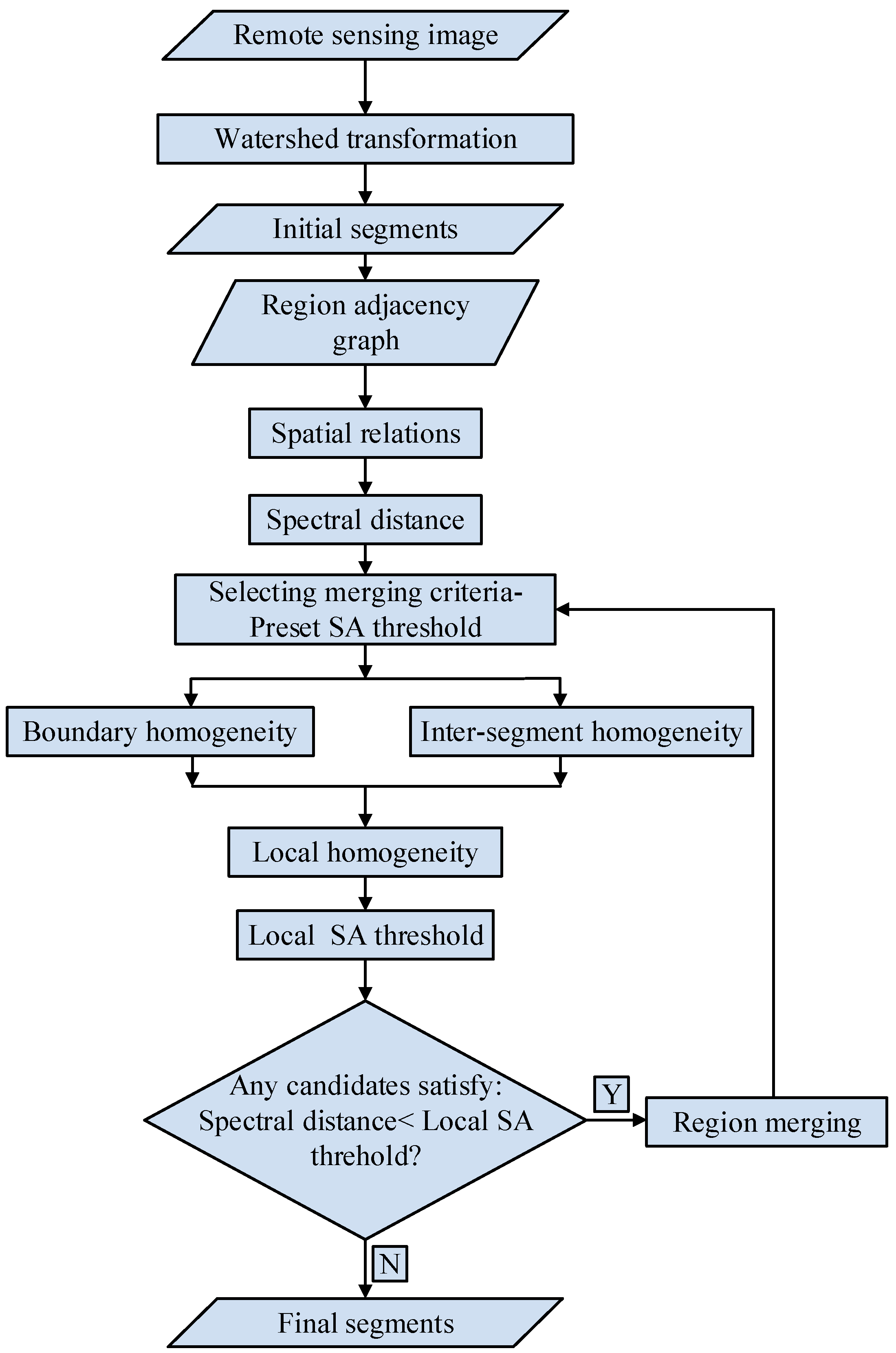
2. Methodology
2.1. Initial Segmentation
2.2. Merging Criteria
2.3. Local Adaptive SA Threshold Aided by Inter-Segment and Boundary Homogeneities
2.4. Region Merging Using Adjusted Local SA Threshold
2.5. Segment Evaluation
3. Experiment Setups
3.1. Data Sets
3.2. Methods for Comparison
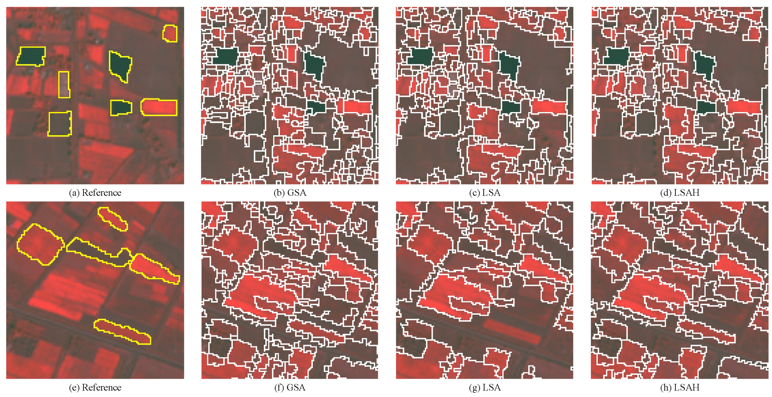
4. Results
4.1. Farmland Area
4.2. Urban Area
4.3. Rural Area
5. Discussion
6. Conclusions
Author Contributions
Funding
Acknowledgments
Conflicts of Interest
References
- Blaschke, T.; Hay, G.J.; Kelly, M.; Lang, S.; Hofmann, P.; Addink, E.; Feitosa, R.Q.; Meer, F.V.D.; Werff, H.V.D.; Coillie, F.V. Geographic Object-Based Image Analysis—Towards a new paradigm. ISPRS J. Photogramm. Remote Sens. 2014, 87, 180–191. [Google Scholar] [CrossRef] [PubMed]
- Chen, G.; Weng, Q.; Hay, G.J.; He, Y. Geographic object-based image analysis (GEOBIA): Emerging trends and future opportunities. Gisci. Remote Sens. 2018, 55. [Google Scholar] [CrossRef]
- Blaschke, T.; Lang, S.; Hay, G. Object-Based Image Analysis: Spatial Concepts For Knowledge-Driven Remote Sensing Applications; Springer Science & Business Media: Berlin, Germany, 2008. [Google Scholar]
- Lang, S. Object-Based Image Analysis for Remote Sensing Applications: Modeling Reality—Dealing with Complexity; Springer: Berlin, Germany, 2008; pp. 3–27. [Google Scholar]
- Blaschke, T. Object based image analysis for remote sensing. ISPRS J. Photogramm. Remote Sens. 2010, 65, 2–16. [Google Scholar] [CrossRef] [Green Version]
- Conrad, O.; Bechtel, B.; Bock, M.; Dietrich, H.; Fischer, E.; Gerlitz, L.; Wehberg, J.; Wichmann, V.; Böhner, J. System for Automated Geoscientific Analyses (SAGA) v. 2.1.4. Geosci. Model Dev. Discuss. 2015, 8, 2271–2312. [Google Scholar] [CrossRef]
- Berhane, T.M.; Lane, C.R.; Wu, Q.; Anenkhonov, O.A.; Chepinoga, V.V.; Autrey, B.C.; Liu, H. Comparing Pixel-and Object-Based Approaches in Effectively Classifying Wetland-Dominated Landscapes. Remote Sens. 2017, 10, 46. [Google Scholar] [CrossRef] [PubMed]
- Inglad, J. Automatic recognition of man-made objects in high resolution optical remote sensing images by SVM classification of geometric image features. ISPRS J. Photogramm. Remote Sens. 2007, 62, 236–248. [Google Scholar] [CrossRef]
- Jia, H.; Xing, Z.; Song, W. Three Dimensional Pulse Coupled Neural Network Based on Hybrid Optimization Algorithm for Oil Pollution Image Segmentation. Remote Sens. 2019, 11, 1046. [Google Scholar] [CrossRef]
- Trias-Sanz, R.; Stamon, G.; Louchet, J. Using colour, texture, and hierarchial segmentation for high-resolution remote sensing. ISPRS J. Photogramm. Remote Sens. 2008, 63, 156–168. [Google Scholar] [CrossRef]
- Radoux, J.; Bourdouxhe, A.; Coos, W.; Dufrêne, M.; Defourny, P. Improving Ecotope Segmentation by Combining Topographic and Spectral Data. Remote Sens. 2019, 11, 354. [Google Scholar] [CrossRef]
- Canny, J. A Computational Approach to Edge Detection. In Readings in Computer Vision; Morgan Kaufmann: San Francisco, CA, USA, 1987; pp. 184–203. [Google Scholar]
- Bischof. Seeded Region Growing. IEEE Trans. Pattern Anal. Mach. Intell. 2002, 16, 641–647. [Google Scholar]
- Chen, B.; Qiu, F.; Wu, B.; Du, H. Image Segmentation Based on Constrained Spectral Variance Difference and Edge Penalty. Remote Sens. 2015, 7, 5980–6004. [Google Scholar] [CrossRef] [Green Version]
- Baatz, M. Multi resolution Segmentation: An optimum approach for high quality multi scale image segmentation. In Beutrage zum AGIT-Symposium; Springer: Salzburg, Germany, 2000; pp. 12–23. [Google Scholar]
- Liu, J.; Li, P.; Wang, X. A new segmentation method for very high resolution imagery using spectral and morphological information. ISPRS J. Photogramm. Remote Sens. 2015, 101, 145–162. [Google Scholar] [CrossRef]
- Pavlidis, T.; Liow, Y.T. Integrating region growing and edge detection. IEEE Trans. Pattern Anal. Mach. Intell. 1990, 12, 225–233. [Google Scholar] [CrossRef]
- Cortez, D.; Nunes, P.; Sequeira, M.M.D.; Pereira, F. Image segmentation towards new image representation methods. Signal Process. Image Commun. 1995, 6, 485–498. [Google Scholar] [CrossRef]
- Zhang, X.; Xiao, P.; Feng, X. Fast Hierarchical Segmentation of High-Resolution Remote Sensing Image with Adaptive Edge Penalty. Photogramm. Eng. Remote Sens. 2015, 80, 71–80. [Google Scholar] [CrossRef]
- Zhang, X.; Xiao, P.; Feng, X.; Wang, J.; Wang, Z. Hybrid region merging method for segmentation of high-resolution remote sensing images. ISPRS J. Photogramm. Remote Sens. 2014, 98, 19–28. [Google Scholar] [CrossRef]
- Mitra, P.; Shankar, B.U.; Pal, S.K. Segmentation of multispectral remote sensing images using active support vector machines. Pattern Recognit. Lett. 2004, 25, 1067–1074. [Google Scholar] [CrossRef]
- Beucher, S.; Mathmatique, C.D.M. The Watershed Transformation Applied To Image Segmentation. Scanning Microsc. Suppl. 1992, 6, 299–314. [Google Scholar]
- Toro, C.; Martín, C.; Pedrero, A.; Ruiz, E. Superpixel-Based Roughness Measure for Multispectral Satellite Image Segmentation. Remote Sens. 2015, 7, 14620–14645. [Google Scholar] [CrossRef] [Green Version]
- Benz, U.C.; Hofmann, P.; Willhauck, G.; Lingenfelder, I.; Heynen, M. Multi-resolution, object-oriented fuzzy analysis of remote sensing data for GIS-ready information. ISPRS J. Photogramm. Remote Sens. 2004, 58, 239–258. [Google Scholar] [CrossRef]
- Comaniciu, D.; Meer, P. Mean shift: A robust approach toward feature space analysis. IEEE Trans Pattern Anal. Mach. Intell. 2002, 24, 603–619. [Google Scholar] [CrossRef]
- Su, T. A novel region-merging approach guided by priority for high resolution image segmentation. Remote Sens. Lett. 2017, 8, 771–780. [Google Scholar] [CrossRef]
- Yang, J.; He, Y.; Weng, Q. An Automated Method to Parameterize Segmentation Scale by Enhancing Intrasegment Homogeneity and Intersegment Heterogeneity. IEEE Geosci. Remote Sens. Lett. 2015, 12, 1282–1286. [Google Scholar] [CrossRef]
- Wang, Y.; Meng, Q.; Qi, Q.; Yang, J.; Liu, Y. Region Merging Considering Within- and Between-Segment Heterogeneity: An Improved Hybrid Remote-Sensing Image Segmentation Method. Remote Sens. 2018, 10, 781. [Google Scholar] [CrossRef]
- Yang, J.; He, Y.; Caspersen, J. Region merging using local spectral angle thresholds: A more accurate method for hybrid segmentation of remote sensing images. Remote Sens. Environ. 2017, 190, 137–148. [Google Scholar] [CrossRef]
- Yang, J.; He, Y.; Caspersen, J. A multi-band watershed segmentation method for individual tree crown delineation from high resolution multispectral aerial image. In Proceedings of the 2014 IEEE Geoscience and Remote Sensing Symposium, Quebec City, QC, Canada, 13–18 July 2014; pp. 1588–1591. [Google Scholar]
- Li, P.; Guo, J.; Song, B.; Xiao, X. A Multilevel Hierarchical Image Segmentation Method for Urban Impervious Surface Mapping Using Very High Resolution Imagery. IEEE J. Sel. Top. Appl. Earth Obs. Remote Sens. 2011, 4, 103–116. [Google Scholar] [CrossRef]
- Kruse, F.A.; Lefkoff, A.; Boardman, J.; Heidebrecht, K.; Shapiro, A.; Barloon, P.; Goetz, A. The spectral image processing system (SIPS)—interactive visualization and analysis of imaging spectrometer data. Remote Sens. Environ. 1993, 44, 145–163. [Google Scholar] [CrossRef]
- Vincent, L.; Soille, P. Watersheds in Digital Spaces: An Efficient Algorithm Based on Immersion Simulations. IEEE Trans. Pattern Anal. Mach. 1991, 13, 583–598. [Google Scholar] [CrossRef]
- Trémeau, A.; Colantoni, P. Regions adjacency graph applied to color image segmentation. IEEE Trans. Image Process 2002, 9, 735–744. [Google Scholar] [CrossRef]
- Zhang, X.; Feng, X.; Xiao, P.; He, G.; Zhu, L. Segmentation quality evaluation using region-based precision and recall measures for remote sensing images. ISPRS J. Photogramm. Remote Sens. 2015, 102, 73–84. [Google Scholar] [CrossRef]
- Su, T.; Zhang, S. Local and global evaluation for remote sensing image segmentation. ISPRS J. Photogramm. Remote Sens. 2017, 130, 256–276. [Google Scholar] [CrossRef]
- Clinton, N.; Holt, A.; Scarborough, J.; Yan, L.; Gong, P. Accuracy Assessment Measures for Object-based Image Segmentation Goodness. Photogramm. Eng. Remote Sens. 2010, 76, 289–299. [Google Scholar] [CrossRef]
- Weidner, U. Contribution to the assessment of segmentation quality for remote sensing applications. Int. Arch. Photogramm. Remote Sens. Spat. Inf. Sci. 2008, 37, 479–484. [Google Scholar]
- Benedek, C.; Descombes, X.; Zerubia, J. Building Development Monitoring in Multitemporal Remotely Sensed Image Pairs with Stochastic Birth-Death Dynamics. IEEE Trans. Pattern Anal. Mach. Intell. 2012, 34, 33–50. [Google Scholar] [CrossRef]
- Grinias, I.; Panagiotakis, C.; Tziritas, G. MRF-based segmentation and unsupervised classification for building and road detection in peri-urban areas of high-resolution satellite images. ISPRS J. Photogramm. Remote Sens. 2016, 122, 145–166. [Google Scholar] [CrossRef]
- Chen, R.; Li, X.; Li, J. Object-Based Features for House Detection from RGB High-Resolution Images. Remote Sens. 2018, 10, 451. [Google Scholar] [CrossRef]
- Shepherd, J.D.; Bunting, P.; Dymond, J.R. Operational Large-Scale Segmentation of Imagery Based on Iterative Elimination. Remote Sens. 2019, 11, 658. [Google Scholar] [CrossRef]
- Basaeed, E.; Bhaskar, H.; Hill, P.; Al-Mualla, M.; Bull, D. A supervised hierarchical segmentation of remote-sensing images using a committee of multi-scale convolutional neural networks. Int. J. Remote Sens. 2016, 37, 1671–1691. [Google Scholar] [CrossRef] [Green Version]
- Fu, Z.; Sun, Y.; Fan, L.; Han, Y. Multiscale and Multifeature Segmentation of High-Spatial Resolution Remote Sensing Images Using Superpixels with Mutual Optimal Strategy. Remote Sens. 2018, 10, 1289. [Google Scholar] [CrossRef]


| Input data: Initial segmentation |
| Input parameter: Spectral angel |
| Procedure |
|
| Output: Final segmentation result |
| Reference Polygon | Average Area | Min Area | Max Area | Main Land Cover Types | |
|---|---|---|---|---|---|
| Numbers | (Pixel) | (Pixel) | (Pixel) | of the Reference Polygons | |
| farmland | 50 | 234.56 | 23 | 975 | Building, Water |
| Cropland, Open field | |||||
| urban | 50 | 369.39 | 12 | 2006 | Building, Road, Woods |
| Open field, Asphalt | |||||
| rural | 50 | 175.34 | 14 | 825 | Building, Open field, Woods |
| Asphalt, Grass, Water, Cropland |
© 2019 by the authors. Licensee MDPI, Basel, Switzerland. This article is an open access article distributed under the terms and conditions of the Creative Commons Attribution (CC BY) license (http://creativecommons.org/licenses/by/4.0/).
Share and Cite
Zhang, Y.; Wang, X.; Tan, H.; Xu, C.; Ma, X.; Xu, T. Region Merging Method for Remote Sensing Spectral Image Aided by Inter-Segment and Boundary Homogeneities. Remote Sens. 2019, 11, 1414. https://doi.org/10.3390/rs11121414
Zhang Y, Wang X, Tan H, Xu C, Ma X, Xu T. Region Merging Method for Remote Sensing Spectral Image Aided by Inter-Segment and Boundary Homogeneities. Remote Sensing. 2019; 11(12):1414. https://doi.org/10.3390/rs11121414
Chicago/Turabian StyleZhang, Yuhan, Xi Wang, Haishu Tan, Chang Xu, Xu Ma, and Tingfa Xu. 2019. "Region Merging Method for Remote Sensing Spectral Image Aided by Inter-Segment and Boundary Homogeneities" Remote Sensing 11, no. 12: 1414. https://doi.org/10.3390/rs11121414