Article

Quantitative Analysis of Spectral Response to Soda Saline-AlkaliSoil after Cracking Process: A Laboratory Procedure to Improve Soil Property Estimation

1
Heilongjiang Province Key Laboratory of Geographical Environment Monitoring and Spatial Information Service in Cold Regions, Harbin Normal University, Harbin 150025, China
2
Northeast Institute of Geography and Agroecology, Chinese Academy of Sciences, Changchun 130102, China
3
State Environmental Protection Key Laboratory of Wetland Ecology and Vegetation Restoration, Northeast Normal University, Changchun 130024, China
4
College of Life Sciences, Henan Normal University, Xinxiang 453007, China
*
Author to whom correspondence should be addressed.
Remote Sens. 2019, 11(12), 1406; https://doi.org/10.3390/rs11121406
Submission received: 18 April 2019 / Revised: 7 June 2019 / Accepted: 10 June 2019 / Published: 13 June 2019
(This article belongs to the Special Issue Monitoring Soil Degradation by Remote Sensing)

Abstract

:
Cracking on the surface of soda saline-alkali soil is very common. In most previous studies, spectral prediction models of soil salinity were less accurate since spectral measurements were usually performed on 2 mm soil samples which cannot represent true soil surface condition very well. The objective of our research is to provide a procedure to improve soil property estimation of soda saline-alkali soil based on spectral measurement considering the texture feature of the soil surface with cracks. To achieve this objective, a cracking test was performed with 57 soil samples from Songnen Plain of China, the contrast (CON) texture feature of crack images of soil samples was then extracted from grey level co-occurrence matrix (GLCM). The original reflectance was then measured and the mixed reflectance considering the CON texture feature was also calculated from both the block soil samples (soil blocks separated by crack regions) and the comparison soil samples (soil powders with 2 mm particle size). The results of analysis between spectra and the main soil properties indicate that surface cracks can reduce the overall reflectivity of the soda saline-alkali soil and thus increasing the spectral difference among the block soil samples with different salinity levels. The results also show that both univariate and multivariate linear regression models considering the CON texture feature can greatly improve the prediction accuracy of main soil properties of soda saline-alkali soils, such as Na+, EC and salinity, which also can reduce the intensity of field spectral measurements under natural condition.

Graphical Abstract

1. Introduction

Soil salinization is one of the most common worldwide land degradation processes, which seriously affects major soil degradation phenomenon such as soil dispersion, soil erosion, and engineering problems, and thus reduces agricultural production, and impacts environmental health [1,2,3,4]. According to Food and Agriculture Organization of the United Nations, the global surface area affected by soil salinization was more than 831 million ha by 2000, covering more than 6% of the Earth’s surface [5]. Therefore, identification of the soil salinity and the salt-affected areas is essential for sustainable agricultural management, especially in arid and semi-arid areas [6,7].
Due to its high temporal sampling frequency and rapid nondestructive measurement, reflectance spectroscopy has been widely used to estimate soil salinity [8,9,10,11,12,13]. Hyperspectral data has become a promising source of data in many studies since it contains a large number of narrow contiguous spectral bands with high spectral resolution and thus enables the quantitative measurement of saline soils with different salinity levels [14,15,16,17]. During the last several decades, many studies have been focused on the effect of salinity on the spectral characteristics of saline soils. Taylor et al. [18] found absorption valleys at 980 nm, 1170 nm, 1450 nm, and 1900 nm, and strong reflection peaks at 800 nm. Farifteh et al. [19] carried out a laboratory experiment involving soils with six salt minerals and three soil textures in order to study the quantitative relationship between spectral response and salt concentration of saline soil samples, their results showed that the observed absorption features were broadened at wavelength above 1300 nm and the overall reflectance changed proportionally as the soil salinity increased. Wang et al. [20] carried out a spectra measurement in of saline soil, the laboratory and found significant absorption features at 505 nm, 920 nm, 1415 nm, 1915 nm, and 2205 nm. Moreira et al. [21] evaluated the variations in spectral reflectance of soil samples treated with different salt crystals using both principal component analysis and the continuum-removed method, after that they found the obvious absorption depths of major features at 1450 nm, 1950 nm, 1750 nm, and 2200 nm, their results also indicated the best negative correlations between reflectance and EC in the 1500–2400 nm range for CaCl2 and MgCl2.
In many studies, spectral indices were commonly used to process the hyperspectral data of saline soil after spectral measurements. Zovko et al. [22] selected 246 soil samples for visible and near-infrared spectra measurements and defined a new geostatistical spectral index as covariate in ordinary cokriging for predicting electrical conductivity, spatial variation of soil salinity was then mapped in the Neretva River Valley, Croatia to propose an effective approach based on VNIR spectroscopy and geostatistics for mapping soil salinity. In order to predict the salt abundance in slightly saline soils in Burg Al-Arab, Egypt, Masoud [23] carried out spectrometry measurements for 21 soil samples with different salinity levels to evaluate the simple wetness index (WI) and sophisticated spectral mixture analysis techniques including mixture tuned matched filtering (MTMF) and linear spectral unmixing (LSU).The prediction results of salinity levels showed significant high accuracy with R2 of 0.88, 0.84 for MTMF, LSU and WI, respectively. After comparing three spectral indices including difference index (DI), normalized difference index (NDI) and ratio index (RI). Nawar et al. [24] developed regression models with the EC in the El-Tina Plain, Egypt, their results showed RI can provide a reliable estimations of the soil EC with produced R2, RMSE and RPD values of 0.8, 6.2, and 2.06.
Due to its superiority in dealing with high dimensional multi-collinearity, partial least square regression (PLSR) has been used as a very common multivariate statistical method in predicting the soil salinity. Weng et al. [25] measured the reflectance spectra (350–2500 nm) from EO-1 Hyperion and tested PLSR as prediction model to evaluate the potential of predicting salt content in the Yellow River Delta of China, their results indicated that spectral bands at 1487–1527 nm, 1971–1991 nm, 2032–2092 nm, and 2163–2355 nm possessed large absolute values of regression coefficients. After collecting in situ field spectra of saline soils in the Yellow River Delta of China, Fan et al. [26] established a PLSR model between soil salinity and field spectra extracted from Advanced Land Imager (ALI), the effectiveness of PLSR model was then demonstrated in retrieving soil salinity from new-generation sensors, their results indicated that the prediction accuracy was quite acceptable with R2, RPD of 0.749, 3.584, respectively. In addition, many other multivariate statistical techniques such as artificial neural networks (ANN), principal component analysis (PCA), and multiple adaptive regression spline (MARS) were used for quantitative determination of soil salinity and illustrating the relationships between spectral characteristics and soil properties [27,28,29]. Although the spectral characteristics of soil samples can reflect the difference of soil salt content to a certain degree, only soil samples after grinding over 2 mm sieve were used in most previous spectral measurements, which usually cannot represent the true surface state of saline soils. For many saline soils with complex surface conditions or high roughness, spectral measurement of 2mm soil samples often cannot give a good estimation of salt content.
For saline soil samples, especially for those soda saline-alkali soils with relatively high clay content, it is very common to shrink and crack for the soil surface during water evaporation. Volume scattering was generated in the crack regions and result in a significant mixed pixel spectral effect. However, studies on the correlation between salt content and the overall spectral reflectance of saline soils with desiccation cracks are still limited and qualitative [30,31]. Texture features always contain important information about the structural arrangement of the soil surface with desiccation cracks, which can also accurately reflect the hue information and the overall arrangement of crack patterns [32,33,34,35]. However, spectral measurements considering the texture features of soil surface cracks were rarely focused on. To address this gap, the quantitative relationship between the reflectance spectra and soil properties of soda saline-alkali soils were tried to be analyzed based on consideration of the grey level co-occurrence matrix (GLCM) texture feature. Optimal predictive models for four main soil properties of interest including Na+, EC, pH and total salinity were also developed based on the original reflectance and the mixed reflectance considering the contrast texture feature (CON) for the block soil samples (soil blocks separated by crack regions generated during the desiccation cracking process) and the comparison soil samples (soil powders with 2 mm particle size) respectively. This can be used to improve the prediction accuracy of soil salinity with less work intensity of soil spectral measurement in field conditions.

2. Materials and Methods

2.1. Study Area and Sampling

Songnen Plain contains one of the most three largest amounts of heavy soda salt-affected soils in the world. The main salt components of saline soils are NaHCO3 and Na2CO3, which make the soils very sodic [36]. This study was conducted from 2013 to 2014 with all soil samples obtained in 12 towns of Da’an City, which is located on the southwestern Songnen Plain, Jilin Province, China with the geographic coordinates lie between 123°47’35’’E~123°59’55’’E and 45°29’30’’N~45°36’26’’N. The annual mean precipitation of this area is approximately 400~500 mm with 80% occurs between June and September, while the average annual evaporation is about 1400~1900 mm, reaching 3.5 to 4.75 times of precipitation. Moreover, the soil clay content in the study area is quite high, which makes the soil surface shrink and crack very commonly during water evaporation.
After consideration of heterogeneity, 57 composite soil samples of different salinity levels were collected at a depth of 20 cm in July 2013, April and October 2014. Figure 1a,b shows the study area location and the spatial coordinates of all sampling locations recorded using a hand-held GPS. The soil surface from Figure 1c–e indicates that it is very common to crack on the surface of soda saline-alkali soils in Songnen Plain. All soil samples were air-dried, ground, passed through a 2 mm sieve and then divided into three subsamples. The first subsamples were prepared for the physical and chemical properties. The second subsamples were prepared as the block soil samples the third subsamples were prepared as comparison soil samples for spectral collection.

2.2. Soil Property Measurement

The main ions, such as K+, Na+, Mg2+, Ca2+, Cl, CO32− and HCO3 were measured in a laboratory. Soil extracts with water/soil mass ratio of 1:5 were used to measure the contents of Na+ and K+ using a flame photometer. The contents of Ca2+ and Mg2+ were determined by the complexometric ethylenediaminetetraacetic acid (EDTA) titration method. The contents of CO32− and HCO3 were obtained based on the double indicator neutralization method. Moreover, EC and pH were also measured by the potentiostatic method and conductometry, using soil suspensions with a soil/water mass ratio of 1:5 [37]. In addition, a Malvern MS-200 laser particle size analyzer was used in this study to determine the contents of clay, silt, and sand of the soil samples [38].

2.3. Desiccation Cracking Test

In order to remove the effects of environmental factors, the desiccation cracking process of soda saline-alkali soils was carried out under controlled experimental conditions. Saturated slurry samples were firstly prepared with a mass water content of 80% using the subsamples treated previously. The obtained slurry samples were then well hand-mixed and poured into wooden sample box of 50 cm × 50 cm × 3 cm size with the top flattened by a spatula. Afterwards, all soil samples were subjected in the laboratory with temperature of 25 °C, humidity of 35% and pressure of 101 kPa, and the soil samples were then air-dried until masses no longer decreased, which can be considered as completely dried samples. The gravimetric water contents of the soil samples were then measured. In order to obtain the crack images of soil samples, a digital camera was installed on a fixed experimental platform. The lens of the digital camera was set 1 m above the floor. A 50 cm × 50 cm square area was determined with the projection of the camera lens on the floor as the center, which was used to ensure that the geometric distortion effects were the same for all the samples during the photographing process. Each cracked soil specimen was then placed in the determined square area to be photographed (Figure 2).

2.4. Texture Feature Extraction

The CON is an important GLCM texture feature, which can well express the clarity and reflect the intensity of the texture of adjacent pixels of crack patterns, thus the CON is considered as an important measure of local variations present in crack patterns in this study. The CON can be calculated by the following equation:
C O N = n N g 1 n 2 { i = 1 N g j = 1 N g p ( i , j ) } , | i j | = n
where p(i,j) represents the second-order combined conditional probability density of gray level i and j, corresponding to the element of GLCM at (i,j) position. For an Lr × Lc grayscale image with gray level of Ng and sampling interval of d pixels, p(i,j)at directions of 0°, 45°, 90°, and 135° can be computed by the following equations separately [39,40,41,42]:
p ( i , j , d , 0 ° ) = # { ( x 1 , y 1 ) , ( x 2 , y 2 ) ( L r L c ) ( L r L c ) } with   x 1 x 2 = 0 ,   | y 1 y 2 | = d , and   f ( x 1 , y 1 ) = i , f ( x 2 , y 2 ) = j
p ( i , j , d , 45 ° ) = # { ( x 1 , y 1 ) , ( x 2 , y 2 ) ( L r L c ) ( L r L c ) } with   x 1 x 2 = d ,   y 1 y 2 = d , or   x 1 x 2 = d , y 1 y 2 = d and   f ( x 1 , y 1 ) = i , f ( x 2 , y 2 ) = j
p ( i , j , d , 90 ° ) = # { ( x 1 , y 1 ) , ( x 2 , y 2 ) ( L r L c ) ( L r L c ) } with   | x 1 x 2 | = d ,   y 1 y 2 = 0 , and   f ( x 1 , y 1 ) = i , f ( x 2 , y 2 ) = j
p ( i , j , d , 135 ° ) = # { ( x 1 , y 1 ) , ( x 2 , y 2 ) ( L r L c ) ( L r L c ) } with   x 1 x 2 = d ,   y 1 y 2 = d , or   x 1 x 2 = d , y 1 y 2 = d and   f ( x 1 , y 1 ) = i , f ( x 2 , y 2 ) = j
In this study, the crack images were transformed into binary images (Ng = 2) considering the effects of the salt crystals separated out on the surface of soil samples. In detail, to determine the CON of dried soil samples from crack patterns, digital image processing technique was carried out in this study (Figure 3). Firstly, the crack pattern of the cracked soil samples was geometry corrected using polynomial methods and cropped (Figure 3a).After that, the corrected color image was transformed into a gray image (Figure 3b).Thirdly, the grayscale image was binarized using a threshold (Figure 3c) and then inversed for further processing (Figure 3d), which indicated that the crack pattern was segmented into white crack areas and black block areas. Finally, the open operation was then performed with a given threshold to reduce the small spot noise in every binary image (Figure 3e). After the above processes, a distance of 40 pixels was selected as sampling interval in order to fully preserve the GLCM texture information and reduce the computational complexity, the mean CON texture features of all cracked soil samples were then computed based on the CON computed from GLCMs in 0°, 45°, 90°, and 135° directions [43].

2.5. Spectral Features Acquisition

In order to obtain the spectral characteristics of both the block soil samples and the comparison soil samples, an ASD FieldSpec3 hand-held spectrometer produced by Analytical Spectral Devices Inc. was used in this experiment, which was widely used in the spectral measurements of vegetation and soil. This spectrometer covers wavelengths between 350–2500 nm with two separate detectors namely VNIR (visible and near-infrared, 350–1000 nm) and SWIR (short-wave infrared, 1000–2500 nm), it can savethe spectral data and display the spectral curve of the objects. The sampling intervals are 1.4 nm with a spectral resolution of 3 nm and 2 nm for VNIR, and with a spectral resolution of 10 nm SWIR, respectively. All spectral reflectance was measured in clear and cloudless weather conditions.
For both block and comparison soil samples, the spectrometer with an 8° field of view was held on a fixed platform 10 cm vertically above the surface of soil samples to ensure that the zenith angle and the azimuth angle were kept the same, the corresponding measurement area is then determined as a circle area with a very small radius of 0.7 cm. After that, each soil sample was put uniformly right on a 1m×1m blackboard on the ground in order to minimize the effects of the background and the adjacent objects. 10 randomly spots on the surface of soil samples were then chosen as the center, and the spectral measurements were carried out. Note that before spectral measurements, all comparison soil samples were firstly put in the same aluminum boxes with an inner diameter of 10 cm and a depth of 2 cm (1.5 cm of soil can be considered as infinite thickness in optical remote sensing) and then flattened with a spatula to remove the effect of compaction on the spectral reflectance. During spectral measurement of each soil sample, 10 readings of spectral reflectance were taken, and the mean of all spectral reflectance was calculated as the actual reflectance in order to average out the difference caused by instrument noise. A standard white panel was also measured as calibration before each spectral measurement. In order to diminish the noise of the equipment and further reduce the data dimensions, the spectral reflectance was resampled at 10 nm for all the block and comparison soil samples.

3. Results

3.1. Soil Properties

Table 1 lists the statistical characteristics of the soil properties of soil samples. The total salinity is the sum of ion content. Na+ is the main cation while HCO3 and CO32− are the main anions. Table 1 shows that the EC of the experimental samples ranges from 0.06 ds/m to 3.39 ds/m and the pH of the experimental samples ranges from 8.01 to 10.77, indicating that all the soil samples exhibit alkaline characteristics [44]. Table 1 also shows that there are significant differences in the overall salinity among the soil samples. The salinity of the experimental samples ranges from 1.06 mg/g to 29.73 mg/g, and the ion contents also indicate relatively large differences among different samples. In addition, the standard deviation and coefficient of variation shows that there are relatively large differences in the salt parameters in all the soil samples, in particular, the Cl content, Na+ content, CO32− content, HCO3 content, ECs and salinity all have large coefficients of variation, indicating that the sample point selection accurately reflects the distribution range of the salt parameters. Furthermore, the differences of particle size distributions of the soil samples are very small especially for those particles with clay content <0.005mm, the CV and standard are 5.49% and 1.54 mg/g, which means no significant differences were observed in the clay content for the soil samples.

3.2. CON Texture Features

Figure 4 shows the distributions of the CON texture feature calculated from the crack images of soil samples, which indicates a very large heterogeneity among different soil samples with CON ranges from 0.007 to 0.342.

3.3. Spectral Characteristics

In order to study the spectral response of soda saline-alkali soil to salt contents of both block soil samples and comparison soil samples, sample 29, sample 8, sample 35, sample 43, sample 28 and sample 21 were selected according to the distribution of total salinity at an interval of 5 mg/g, the corresponding salinities were 5.17 mg/g, 10.37mg/g, 15.47mg/g, 20.71mg/g, 25.62mg/g, 29.73 mg/g respectively. The reflectance curves of the above soil samples are shown in Figure 5. From Figure 5a,b, it can be seen that the overall reflectance curves of both block soil samples and comparison soil samples are relatively low in the visible region. The spectral reflectance increases from 350 to 1400 nm and turns basically flat between 1400 and 2200 nm, and then the reflectance curve gradually decreases with the increasing salinity. Figure 5a,b also indicates that the block soil samples are more capable distinguishing the soil salinity compared with the comparison soil samples, the higher the salinity, the lower the reflectance curve. In the sensitive wavelengths above 1400 nm, the spectral curve difference of the block soil samples becomes smaller, and the reflectance interval is more uniform. In addition, Figure 5c,d illustrates the difference in spectra between the block soil sample and the comparison soil sample at the same salinity, it can also be seen that the reflectance curve of the block soil sample is significantly lower than that of the comparison soil sample for both the highest salinityand the lowest salinity.

3.4. Correlation Analysis

In order to extract the optimum reflectance and the corresponding diagnostic wavelengths for developing prediction models with high accuracy, correlograms were calculated in this study across seven soil properties of particular interest (four main ions including Na+, Cl, HCO3, CO32−, total salinity, pH and EC) for reflectance of soil samples under different soil surface conditions. The correlograms can display absolute value curves of the correlation coefficient between a given soil property and spectral reflectance as a function of wavelength (Figure 6).
Figure 6a indicates that for the block soil samples, the shapes of correlation coefficient curves for EC, Na+, Cl, and salinity are basically the same, with an upward trend from 350 to 1400 nm and a small peak near 500 nm. The correlation between soil parameters and reflectivity decreases firstly and then increases between 1400 nm and 1900 nm, but the change is not obvious. The curve remains basically flat with a small uplift around 1900 nm, and then slightly decreases. The maximum value of the correlation coefficient appears at 1990 nm. For CO32−, the shape of the correlation coefficient curve is nearly the same as EC, Na+, Cl and salinity from 350 to 1400 nm, but appears opposite trend from 1400 to 2500 nm. The curve shapes of HCO3 and pH are basically the same, show a downward trend below 1400 nm and a small absorption valley around 1000 nm. The correlation coefficient curves of HCO3 and pH show a trend of decreasing first and then increasing from 1400 to 2500 nm. The correlation between pH and reflectance is significantly lower than that of HCO3. This is because the pH is determined by the OH content produced by the CO32− and HCO3 hydrolysis reaction, which is often incomplete and reversible due to conditions including temperature and water content. Therefore, in the sensitive band above 1400 nm, the correlation between HCO3 and pH and the spectral reflectance is quite poor, but the overall trend of correlograms is still the same as that of salinity. Figure 6b shows that the correlograms of comparison soil samples are opposite to those of the block soil samples in the visible range from 350 to 650 nm. The correlation coefficient curves of comparison soil samples share the same trends with the block soil samples at the wavelength above 650 nm but with rougher shapes and greater magnitudes. In addition, Figure 6c,d illustrates the difference in coefficient between the block soil samples and the comparison soil samples for salinity and EC, it can be seen that the correlogram curves of the block soil samplesaresignificantly higher than those of the comparison soil samples for both salinity and EC.

3.5. Regression Models

According to Figure 6, the most relevant wavelength was selected at 1990 nm as the diagnostic band, the reflectance of all the block soil samples, and the comparison soil samples was then extracted respectively. Mixed reflectance at 1990 nm was also computed considering the CON texture feature, which was calculated for both the block soil samples and the comparison soil samples based on Equation (6).
R ( λ ) = C O N R 0 ( λ ) + ( 1 C O N ) R 1 ( λ )
where R(λ) represents the mixed reflectance, R0(λ) represents the reflectance of crack regions (ignored in this study), R1(λ) represents the original reflectance of pure soil surface corresponding to the block and the comparison soil samples. In order to effectively predict the soil properties of soda saline-alkali soils and take into account the sufficient reduction of the work intensity, four main soil parameters of interest including Na+, EC, pH, and salinity were selected, both the 57 block soil samples and the 57 comparison soil samples were further arranged according to salinity and evenly selected 38 of them as calibration samples for regression models and other 19 were used for validation. After that, univariate linear regression models were established using both the original reflectance and the mixed reflectance computed from Equation (6), and the results are shown in Table 2. It can be seen from Table 2 that the modeling accuracy using the original reflectance of comparison soil samples is lowest with R2 are only 0.41, 0.39, 0.10 and 0.45 for Na+, EC, pH, and salinity, that the modeling accuracy using the original reflectance of block soil samples is higher with R2 are 0.74, 0.68, 0.23, 0.72 for Na+, EC, pH and salinity. Moreover, the modeling accuracy of the univariate regression model is greatly improved for both the block and the comparison soil samples after considering the CON texture feature.
In order to make full use of the spectral reflectance, 1990 nm, and another three sensitive bands of 990 nm, 1470 nm, and 1990 nm were selected as the characteristic spectrum bands. Multivariate regression models of soil properties were then developed based on both the original reflectance and the mixed reflectance computed from Equation (6) at above four sensitive wavelengths for the block soil samples and the comparison soil samples respectively (Table 3). From Table 3, it can be seen that the modeling accuracy of multivariate linear models for soil properties is higher than that of univariate linear models. Table 3 also indicates that the accuracy based on the original reflectance of comparison soil samples is the poorest with R2 of Na+, EC, pH, and salinity are only 0.44, 0.42, 0.17 and 0.49, that the modeling accuracy using the original block soil samples is higher with R2 are 0.75, 0.70, 0.29, 0.75 for Na+, EC, pH and salinity. In addition, the CON texture feature can also help to improve the modeling accuracy of multivariate regression models for both the comparison soil samples and the block soil samples.

4. Discussion

Many studies have shown that the cracking process of clayey soil is mainly affected by the mechanical properties such as the soil matrix suction, the tensile strength, and the surface energy, these factors generally depend on the mineral type and clay content [45,46,47]. Du et al. [48] and Zhang and Peng [49] have shown that soil clay is an important factor affecting soil shrinkage and cracking process due to its obvious plasticity, swelling, and cohesiveness. Gray and Allbrook [50] found that soil shrinkage and cracking ability is significantly positively correlated with soil clay content. Greene-Kelly [51] showed that soil shrinkage and crack ability is stronger when the expansive clay minerals (such as smectite) dominate in the soil. After measuring the relationship between internal friction angle and cohesion and smectite content, Chen et al. [52] illustrated that when the smectite content is above 5%, the internal friction angle and soil cohesion of soil particles begin to decrease while shrinkage cracking enhances. Zhang et al. [53] carried out X-ray diffraction complete analysis for soil minerals, their measurement results showed that the mineral composition of the saline soils in Songnen Plain is dominated by quartz and feldspar, which accounts for 87.6% to 91.6% of mineral contents, and that only a small amount of kaolinite and almost no highly active smectite is contained. Illite/smectite mixed layer formation is the secondary mineral with an interlaying ratio above 0.5 and the activity index only from 0.33 to 0.48, indicating that the soda saline-alkali soil in Songnen Plain has relatively high compressibility, poor water permeability, low shear strength and limited expansion [54]. From Table 1, it can be seen that although relatively high clay contents (26.28% to 29.37%) were measured in this study, the Std and CV are only 1.54% and 5.49%, this indicates that the clay contents of soil samples are almost the same in this study. On the other hand, the soil sample preparation process was kept the same, and the cracking test was carried out under the same controlled conditions (temperature of 25 °C, humidity of 35% and pressure of 101 kPa), indicating that laboratory conditions also had no effect on the cracking process in this study.
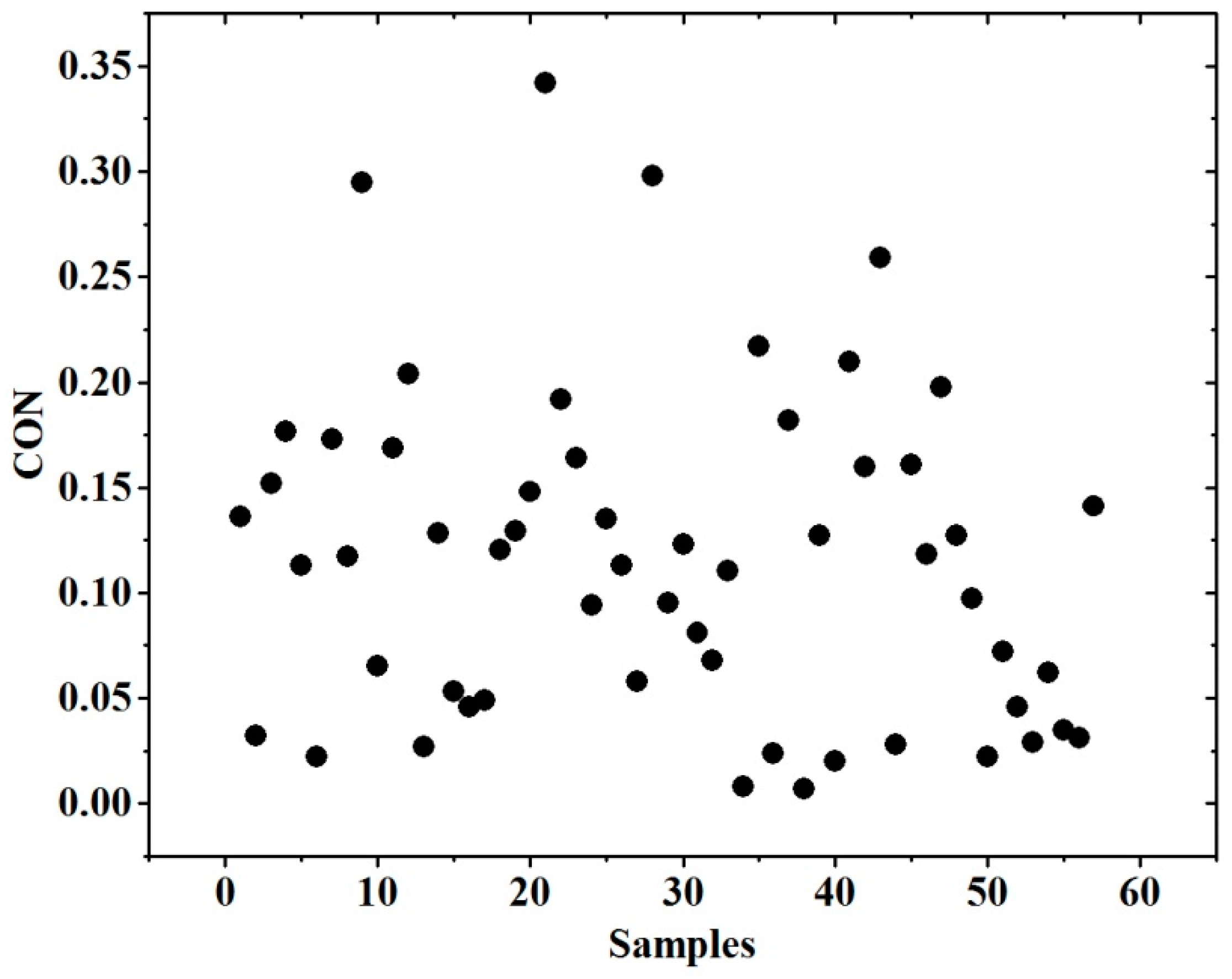
Table 4 shows that the crack degree has a good correlation with the soil properties related to the salt content, the correlation coefficients between the soil properties and the CON are all above 0.68. This is because during the dehydration process of the soil samples, a bounded water film is forming between soil particles (especially Na+ with the large hydrolysis radius) due to the interaction of soil particles with exchangeable cations. The bounded water film reduces the soil cohesion and the tensile strength [55], which also has a great influence on the internal friction angle and the shear strength of the soil [56,57,58]. In addition, the well-known diffuse double layer (DDL) thickness can also be considered as an important role in soil surface cracking, which always becomes thinner as the salt contents of soil samples increase and directly enhances the shrinkage and desiccation cracking of soils during water evaporation [59,60,61].
It can be seen from 
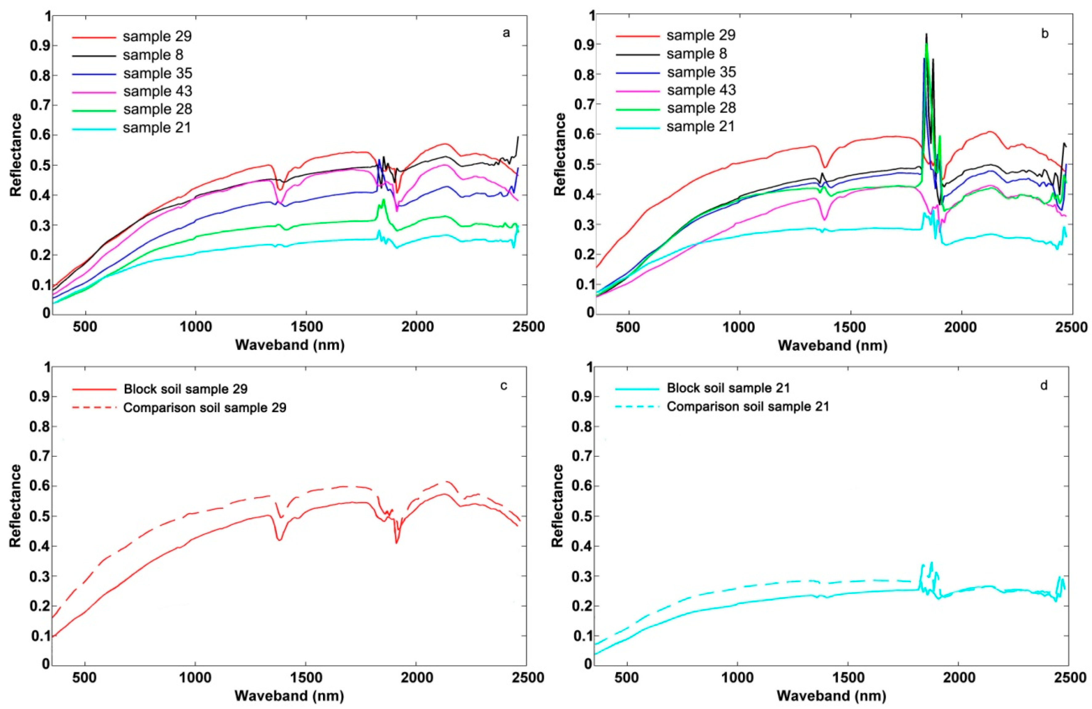
Figure 5 that surface states of soil samples cannot affect the morphology of the reflectance curves but can largely change the amplitudes of the curves. The reflectance curves of the comparison soil samples are higher than those of the block soil samples. This is because after the desiccation cracking process, the area scattering on the surface of block soil samples strengthens with the complexity of surface morphology characterized by the CON texture feature, and the relative surface roughness of block soil samples increases, which reduces the energy reflected to the spectrometer, and thus enhances the spectral difference between different block soil samples. In addition, due to the desiccation cracking test was carried out under natural conditions, all block soil sampleswere air-dried with some residual water remainingin the block soil samples and, therefore, reduced the overall reflectivity compared with the comparison soil samplestotally driedinan oven.Moreover, the shadows appeared within crack regions and made the energy reflect back to the spectrometer close to zero since the incident sunlight was not perpendicular to the surface of the soil samples.
A gradual decrease in reflectance with increasing salt contents was evident, as shown in Figure 5, especially for the wavelength above 1400 nm since NaHCO3and Na2CO3 dominants the salt minerals in Soda saline-alkali soils. Howari et al. [62] and Farifteh et al. [63,64] showed that due to the unique resonance caused by stretching and bending, the sharp decline in reflectance of NaHCO3 and Na2CO3as the wavelength increases can be considered diagnostic since no spectra of other salt minerals were investigated. Similar finding was reported by Wang et al. [65] that the Na2CO3-affected soil has the lowest reflectance shape comparing with saline soils affected by Na2SO4, NaCl and the soil without any salt, their results also indicate that a clear decreasing pattern of reflectance with increasing content of Na2CO3 can be distinguished especially for the wavelength above 1400 nm, which is quite in agreement with the results in this study. Although the residual water contents are very limited (ranging from 0.18% to 2.34% with variance only 0.03%, indicated in Table 5), hygroscopic water can still generate spectral response difference among the block soil samples to a certain extent. This is because from the results studied by Huang et al. [66], salt content can increase the water-holding capacity of soil and thus further reduce the spectral reflectance of soil samples with higher salinities. In addition, according to Tedeschi and Dell’ Aquila [67] and Huang et al., the soil aggregate ability decreases with increasing salinity as a result of the deflocculation of clay colloids induced by the salt, which maybe another reason causing the salinity inversely proportional to the spectral reflectance of the soil samples. Figure 5 also shows that the soil samples under different surface conditions have the same absorption bands and similar corresponding absorption characteristics. Due to the influence of water content in the atmosphere, the reflectance curves exhibit obvious absorption feature at 1900 nm. The reflectance curves also exhibit a weak absorption characteristics of NaCl at 1190 nm, 1150 nm and three weak absorption valleys of NaHCO3 at 1470 nm, 1990 nm and 2170 nm, these weak absorption features are caused by the resonance by the stretching and bending between the ions of the soil salt minerals. The water evaporation during the drying process caused the salt ions to precipitate on the surface of soil samples, making the spectral response to the main soil properties of the block soil samples quite high.
The regression results given in Table 2 and 
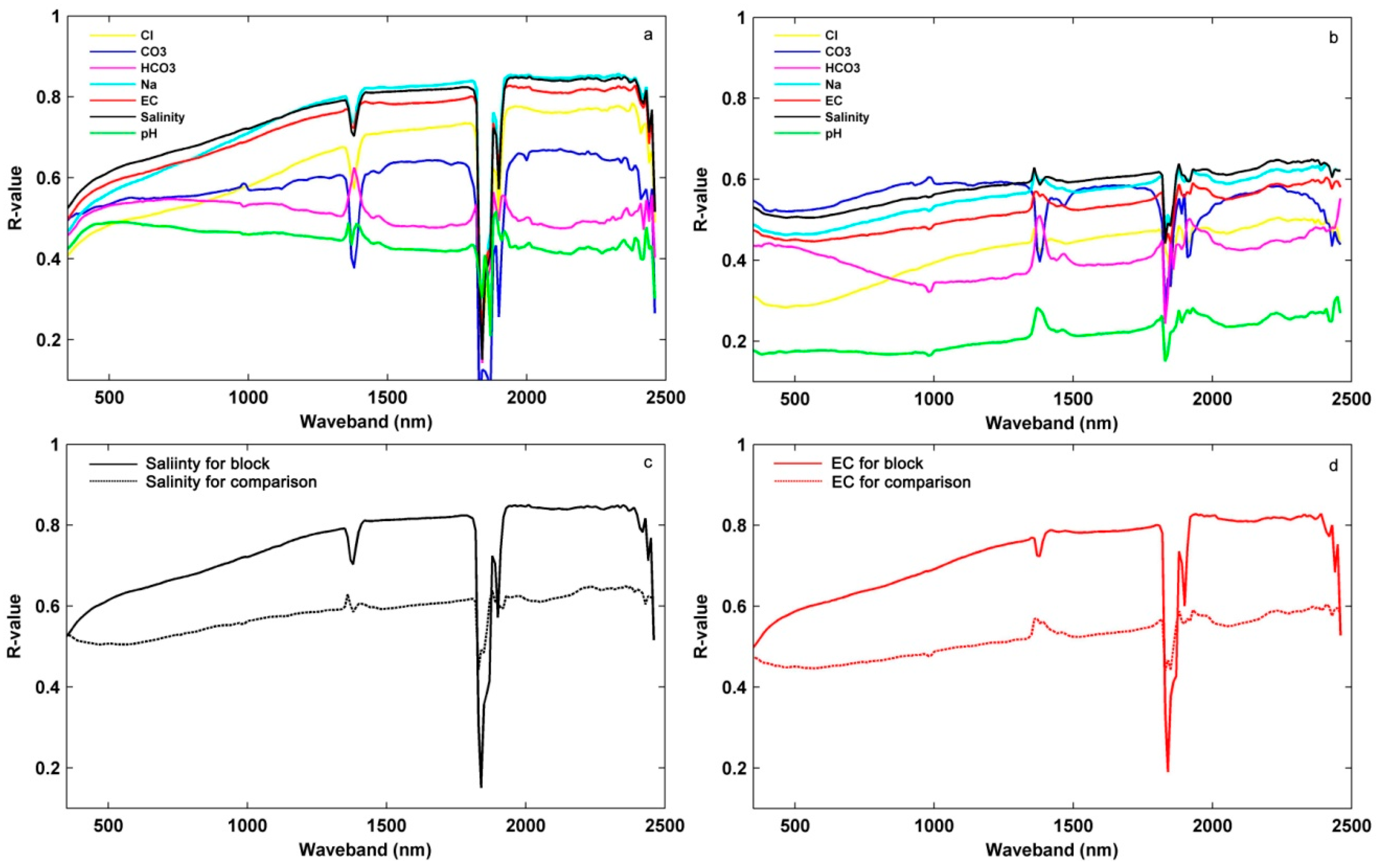
Table 3 indicate that when considering the CON texture feature of crack images, the modeling accuracies of main soil properties can be greatly improved compared with those models developed based on the original reflectance. This is due to the fact that the desiccation cracking process of the soil samples can make the salt separate out on the surface of soil samples, which makes the spectral response of the block soil samples to soil properties stronger than that of the comparison soil samples. Since the reflectance of the crack region is close to zero and the cracking degree is proportional to the salinity of soil samples, a more spectral difference of the block soil samples can be found, and the estimation accuracy of soil properties is, therefore, improved.
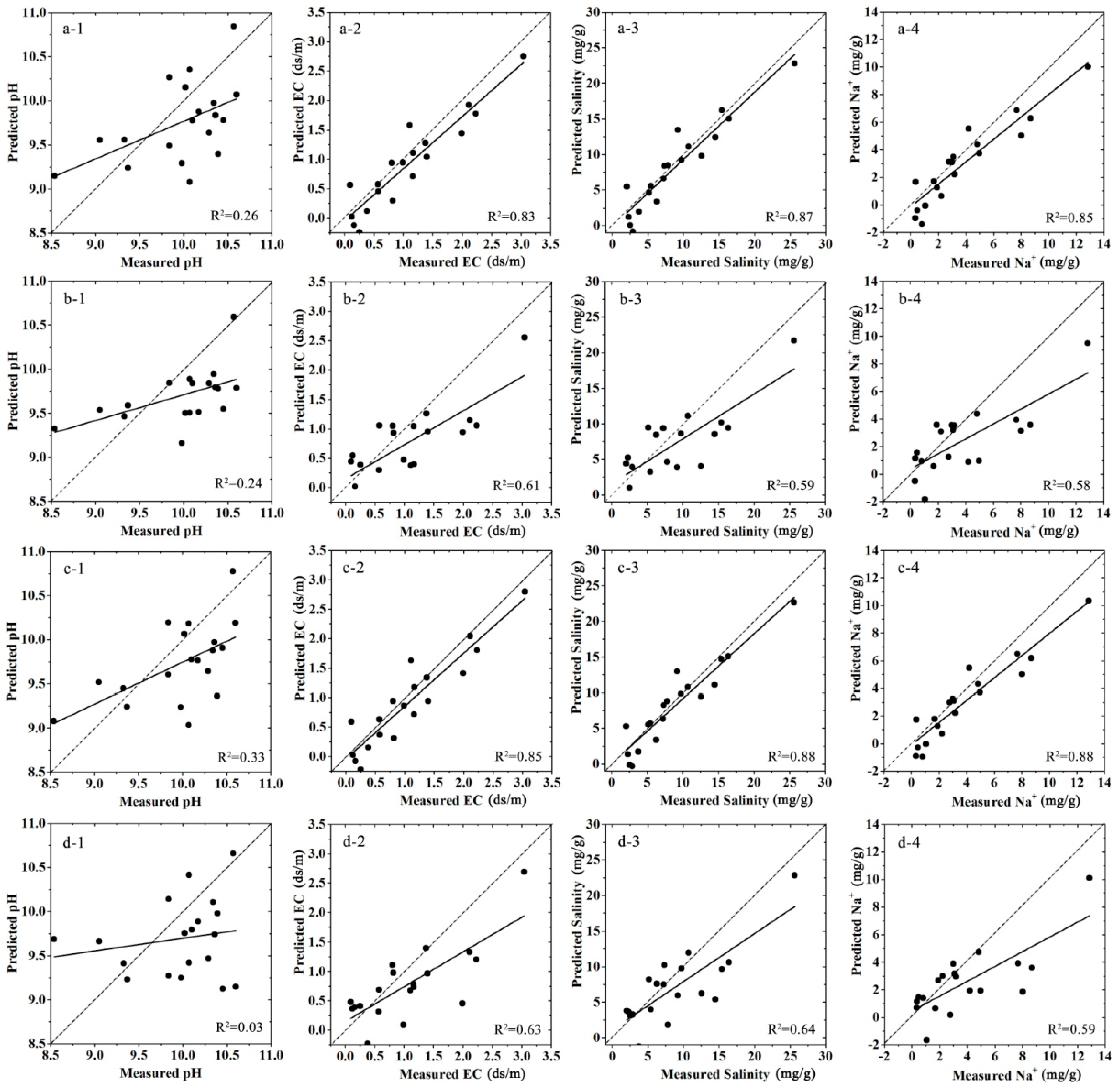
In order to quantitatively evaluate the effectiveness of the regression models considering the CON texture feature, the measured soil properties and the estimated soil properties of all the validation soil samples were linearly fitted to a function of y = x shown in Figure 7. In addition, the root-mean-square error (RMSE), the relative root-mean-square error (RMSE%), the mean absolute error (MAE), the relative mean absolute error (MAE%) and the predicted ratio of deviation (PRD) were calculated as the evaluation indexes, and the results are shown in Table 6. According to the criteria given by Farifteh et al. [68], both univariate and multivariate regression models developed from the block soil samples provide good accuracy for EC, salinity and Na+ (0.82 < R2 < 0.9 and RPD>2), the calculated RMSE, RMSE%, MAE, and MAE% also show that the regression models of EC, salinity and Na+ have quite high reliability and stability. In addition, the univariate and multivariate prediction models developed from the comparison soil samples also show an acceptable prediction accuracy for EC, salinity and Na+ (0.5 < R2 < 0.65 and RPD > 1.5), but high RMSE, RMSE%, MAE The MAE% indicate that the reliability and stability are poor. However, although CON texture features considered, both univariate and multivariate regression models are inaccurate for pH, whether based on the block soil samples or the comparison soil samples.
For the soda saline-alkali soil with surface cracks under natural conditions, the regression models developed in this study can be well implemented to estimate the main soil properties such as EC, salinity and the cation of Na
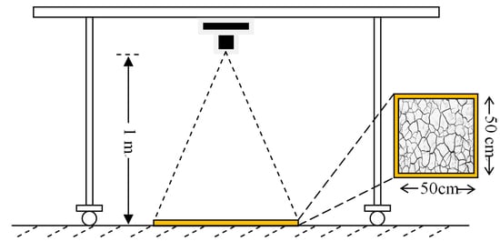
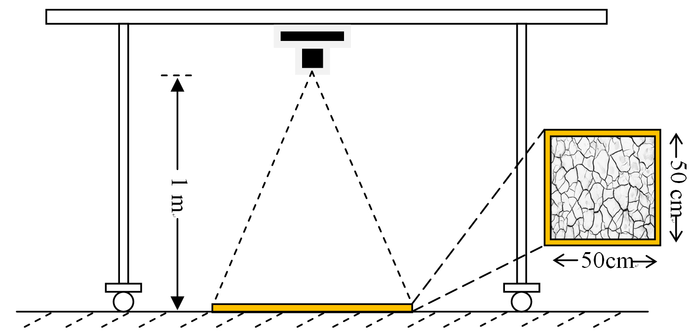
+ with relatively high accuracy and less work intensity. In detail, only soil samples need to be photographed and then collected firstly in the field. Secondly, the spectral measurements can be carried out based on the obtained soil samples (the soil samples collected may be soil blocks or soil powders, corresponding to the block soil samples and the comparison soil samples mentioned in this study) under laboratory-controlled conditions, which usually takes less time than the spectral measurement under natural world. Thirdly, the CON texture features of soil samples with surface cracks can be calculated individually from the crack images obtained in the field. After that, the developed regression models in this study can, therefore, be used for soil properties prediction using the mixed spectral reflectance of the soil samples computed from Equation (6) in Section 3.5. However, the method and the regression linear models developed in this study are still limited for only the salt-affected soil with relatively high clay content, which generates surface cracks commonly under natural conditions. Moreover, other anticipated problems, such as the height of the photograph, the CON scale, the humidity effects, and the atmosphere attenuation, also need to be considered in the field measurement.

5. Conclusions

In this study, a cracking experiment was carried out on 57 samples of soda saline-alkali soil in the Songnen Plain of China. A procedure was studied to improve soil property estimation of soda saline-alkali soil based on spectral measurement considering the CON texture feature of the soil surface with cracks. The spectral response of the block soil samples separated by crack regions and the 2 mm comparison soil samples with different soil properties was analyzed and compared. After that, univariate and multivariate linear regression models were developed for four main soil properties of interest including Na+, EC, pH and total salinity based on the original reflectance and the mixed reflectance considering the CON texture feature for the block soil samples and the comparison soil samples respectively. The main conclusions in this investigation are as follows:
  • The soil salinity can dominate the cracking process of soda saline-alkali soil to a certain extent for the soil with similar clay content and clay mineral composition.
  • The spectral characteristics of the block soil samples are more correlated with soil properties than the comparison soil samples, the mixed reflectance of soil samples considering the CON texture feature can largely improve the prediction accuracy of the main soil properties.
  • Linear regression models based on mixed reflectance considering the CON texture feature of block soil samples show good potential for predicting the main soil properties. For univariate linear regression models, R2 are 0.85, 0.83, 0.87, RPD are 2.81, 4.76, 4.48, for multivariate linear regression models, R2 are 0.88, 0.85, 0.88, RPD are 2.9, 4.81, 4.63.

Author Contributions

Conceptualization, K.Z.; methodology, J.R.; software, J.R.; validation, J.R. and S.L.; formal analysis, J.R.; investigation, X.L. and J.R.; resources, H.Z.; data curation, S.L.; writing—original draft preparation, J.R.; writing—review and editing, X.L.; visualization, X.L. and J.R.; supervision, K.Z.; project administration, J.R.; funding acquisition, J.R.

Funding

This research was supported by the National Natural Science Foundation of China (No. 41601382), the Fundamental Research Funds for the Central Universities of China (No. 2017-KYYWF-0145) and the University Nursing Program for Young Scholars with Creative Talents in Heilongjiang Province of China (No. UNPYSCT-2018180).

Acknowledgments

We are very grateful for the assistance in the soil property measurement provided by Zhichun Wang from the Da’an Alkaline Ecological Experimental Station, Chinese Academy of Sciences.

Conflicts of Interest

The authors declare no conflict of interest.

References

  1. Liu, H.; Xu, J.; Wu, X. Present situation and tendency of saline-alkali soil in west Jilin Province. J. Geogr. Sci. 2001, 11, 321–328. [Google Scholar]
  2. Pankova, E.I. Salt-affected soils of Russia: Solved and unsolved problems. Eurasian Soil Sci. 2015, 48, 115–127. [Google Scholar] [CrossRef]
  3. Daliakopoulos, I.N.; Tsanis, I.K.; Koutroulis, A.; Kourgialas, N.N.; Varouchakis, A.E.; Karatzas, G.P.; Ritsema, C.J. The threat of soil salinity: A European scale review. Sci. Total Environ. 2016, 573, 727–739. [Google Scholar] [CrossRef] [PubMed]
  4. Metternicht, G.I. Soils: Salinization. In The International Encyclopedia of Geography: People, the Earth, Environment and Technology; Wiley-Blackwell: Hoboken, NJ, USA, 2017; pp. 1–10. [Google Scholar]
  5. FAO (Food and Agricultural Organization of the United Nations). Extent and Causes of Salt-Affected Soils in Participating Countries; FAO (Food and Agricultural Organization of the United Nations): Rome, Italy, 2000. [Google Scholar]
  6. Wang, H.; Fan, Y.; Tashpolat, T. The research of soil salinization human impact based on remote sensing classification in oasis irrigation area. Proc. Environ. Sci. 2011, 10, 2399–2405. [Google Scholar]
  7. Singh, Y.P.; Nayak, A.K.; Sharma, D.K.; Singh, G.; Mishra, V.K.; Singh, D. Evaluation of Jatropha curcas genotypes for rehabilitation of degraded sodic lands. Land Degrad. Dev. 2015, 26, 510–520. [Google Scholar] [CrossRef]
  8. Fan, X.; Pedroli, B.; Liu, G.; Liu, Q.; Liu, H.; Shu, L. Soil salinity development in the yellow river delta in relation to groundwater dynamics. Land Degrad. Dev. 2012, 23, 175–189. [Google Scholar] [CrossRef]
  9. Hu, W.; Shao, M.; Wan, L.; Si, B. Spatial variability of soil electrical conductivity in a small watershed on the loess Plateau of China. Geoderma 2014, 230, 212–220. [Google Scholar] [CrossRef]
  10. Allbed, A.; Kumar, L.; Yousef, Y.A. Assessing soil salinity using soil salinity and vegetation indices derived from IKONOS high-spatial resolution imageries: Applications in a data palm dominated region. Geoderma 2014, 230, 1–8. [Google Scholar] [CrossRef]
  11. Li, H.; Webster, R.; Shi, Z. Mapping soil salinity in the Yangtze delta: REML and universal kriging (E-BLUP) revisited. Geoderma 2015, 237, 71–77. [Google Scholar] [CrossRef]
  12. Periasamy, S.; Shanmugam, R.S. Multispectral and microwave remote sensing models to survey soil moisture and salinity. Land Degrad. Dev. 2017, 28, 1412–1425. [Google Scholar] [CrossRef]
  13. Fourati, H.T.; Bouaziz, M.; Benzina, M. Detection of terrain indices related to soil salinity and mapping salt-affected soils using remote sensing and geostatistical techniques. Environ. Monit. Assess. 2017, 189, 177. [Google Scholar] [CrossRef] [PubMed]
  14. Weng, Y.; Gong, P.; Zhu, Z. A spectra index for estimating soil salinity in the Yellow River Delta Region of China using EO-1 Hyperion data. Pedosphere 2010, 20, 378–388. [Google Scholar] [CrossRef]
  15. Bilgili, A.V.; Cullu, M.A.; Vanes, H.; Aydemir, A.; Aydemir, S. The use of hyperspectral visible and near infrared reflectance spectroscopy for the characterization of salt-affected soils in the Harran Plain, Turkey. Arid Soil Res. Rehabil. 2011, 25, 19–37. [Google Scholar] [CrossRef]
  16. Zhang, F.; Tiyip, T.; Ding, J.; Kung, H.; Johnson, V.C.; Sawut, M.; Tashpolat, N.; Gui, D. Studies on the reflectance spectral features of saline soil along the middle reaches of Tarim River: A case study in Xinjiang Autonomous Region, China. Environ. Earth Sci. 2013, 69, 2743–2761. [Google Scholar] [CrossRef]
  17. Sakhaii, P.; Bermel, W. Improving the sensitivity of conventional spin echo spectra by preservation of initial signal-to-noise ratio. J. Magn. Reson. 2014, 242, 220–223. [Google Scholar] [CrossRef] [PubMed]
  18. Taylor, G.R.; Hemphill, P.; Currie, D.; Broadfoot, T.; Dehaan, R.L. Mapping dryland salinity with hyperspectral imagery. In Proceedings of the International Geoscience and Remote Sensing Symposium (IGARSS 2001), Sydney, Australia, 9–13 July 2001; Volume 1, pp. 302–304. [Google Scholar]
  19. Farifteh, J.; van der Meer, F.; van der Meijde, M.; Atzberger, C. Spectral characteristics of salt-affected soils: A laboratory experiment. Geoderma 2008, 145, 196–206. [Google Scholar] [CrossRef]
  20. Wang, Q.; Li, P.; Chen, X. Modeling salinity effects on soil reflectance under various moisture conditions and its inverse application: A laboratory experiment. Geoderma 2012, 170, 103–111. [Google Scholar] [CrossRef]
  21. Moreira, L.C.J.; Teixeira, A.S.; Galvao, L.S. Laboratory salinization of Brazilian alluvial soils and the spectral effects of gypsum. Remote Sens. 2014, 6, 2647–2663. [Google Scholar] [CrossRef]
  22. Zovko, M.; Romic, D.; Colombo, C.; Iorio, E.D.; Romic, M.; Buttafuoco, G.; Castrignano, A. A geostatistical Vis-NIR spectroscopy index to assess the incipient soil salinization in the Neretva River valley, Croatia. Geoderma 2018, 332, 60–72. [Google Scholar] [CrossRef]
  23. Masoud, A.A. Predicting salt abundance in slightly saline soils form Landsat ETM+ imagery using spectral mixture analysis and soil spectrometry. Geoderma 2014, 217–218, 45–56. [Google Scholar] [CrossRef]
  24. Nawar, S.; Buddenbaum, H.; Hill, J. Estimation of soil salinity using three quantitative methods based on visible and near-infrared reflectance spectroscopy: A case study from Egypt. Arab. J. Geosci. 2015, 8, 5127–5140. [Google Scholar] [CrossRef]
  25. Weng, Y.; Gong, P.; Zhu, Z. Soil salt content estimation in the Yellow River Delta with satellite hyperspectral data. Can. J. Remote Sens. 2008, 34, 259–270. [Google Scholar]
  26. Fan, X.; Liu, Y.; Tao, J.; Weng, Y. Soil salinity retrieval from advanced multi-spectral sensor with partial least square regression. Remote Sens. 2015, 7, 488–511. [Google Scholar] [CrossRef]
  27. Zhang, Y.; Hu, P.; Gao, J. A reflectance spectra-based approach to mapping salt fields using PCA-fused Landsat TM data. Adv. Space Res. 2011, 47, 1490–1496. [Google Scholar] [CrossRef]
  28. Sidike, A.; Zhao, S.H.; Wen, Y.M. Estimating soil salinity in Pingluo County of China using QuickBird data and soil reflectance spectra. Int. J. Appl. Earth Obs. Geoinfor. 2014, 26, 156–175. [Google Scholar] [CrossRef]
  29. Nawar, S.; Buddenbaum, H.; Hill, J.; Kozak, J. Modeling and mapping of soil salinity with reflectance spectroscopy and Landsat data using two quantitative methods (PLSR and MARS). Remote Sens. 2014, 6, 10813–10834. [Google Scholar] [CrossRef]
  30. Ren, J.; Zhao, K.; Wu, X.; Zheng, X.; Li, X. Comparative analysis of the spectral response to soil salinity of saline-sodic soils under different surface conditions. Int. J. Environ. Res. Public Health 2018, 15, 2721. [Google Scholar] [CrossRef] [PubMed]
  31. Li, X.; Ren, J.; Zhao, K.; Liang, Z. Correlation between spectral characteristics and physicochemical parameters of soda-saline soils in different states. Remote Sens. 2019, 11, 388. [Google Scholar] [CrossRef]
  32. Lloyd, K.; Rosin, P.L.; Marshall, D.; Moore, S.C. Detecting violent and abnormal crowd activity using temporal analysis of grey co-occurrence matrix (GLCM)-based texture measures. Math. Vis. Appl. 2017, 28, 361–371. [Google Scholar] [CrossRef]
  33. Olaniyi, E.O.; Adekunle, A.A.; Odekuoye, T.; Khashman, A. Automatic system for grading banana using GLCM texture feature extraction and neural network arbitrations. J. Food Eng. 2017, 40, e12575. [Google Scholar] [CrossRef]
  34. Arabi, P.M.; Joshi, G.; Deepa, N.V. Performance evaluation of GLCM and pixel intensity matrix for skin texture analysis. Perspect. Sci. 2016, 8, 203–206. [Google Scholar] [CrossRef] [Green Version]
  35. Malegori, C.; Franzetti, L.; Guidetti, R.; Casiraghi, E.; Rossi, R. GLCM, an image analysis technique for early detection of biofilm. J. Food Eng. 2016, 185, 48–55. [Google Scholar] [CrossRef]
  36. Liang, L.; Li, L.; Liu, Q. Precipitation variability in Northeast China from 1961 to 2008. J. Hydrol. 2011, 404, 67–76. [Google Scholar] [CrossRef]
  37. Bao, S. Agricultural Chemistry Analysis of Soils; Chinese Agriculture Press: Beijing, China, 2000; pp. 152–200. [Google Scholar]
  38. Eshel, G.; Levy, G.J.; Mingelgrin, U. Critical evaluation of the use of laser diffraction for particle-size distribution analysis. Soil Sci. Soc. Am. J. 2004, 68, 736–743. [Google Scholar] [CrossRef]
  39. Rafi, M.; Mukhopadhyay, S. Texture description using multi-scale morphological GLCM. Multimed. Tools Appl. 2018, 77, 30505–30532. [Google Scholar] [CrossRef]
  40. Tan, T.C.Y.; Ritter, L.J.; Whitty, A.; Fernandez, R.C.; Moran, L.J.; Robertson, S.A.; Thompson, J.G.; Brown, H.M. Gray level co-occurrence matrices (GLCM) to assess microstructural and texture changes in pre-implantation embryos. Mol. Reprod. Dev. 2016, 83, 701–713. [Google Scholar] [CrossRef]
  41. Wang, J.; Ren, X. GLCM based extraction of flame image texture features and KPCA-GLVQ recognition method for rotary kiln combustion working conditions. Int. J. Autom. Comput. 2014, 11, 72–77. [Google Scholar] [CrossRef]
  42. Shahbahrami, A.; Pham, T.A.; Bertel, K. Parallel implementation of Gray Level Co-occurrence Matrices and Haralick texture features on cell architecture. J. Supercomput. 2012, 59, 1455–1477. [Google Scholar] [CrossRef]
  43. Ren, J.; Li, X.; Zhao, K.; Fu, B.; Jiang, T. Study of an on-line measurement method for the salt parameters of soda-saline soils based on the texture of features of cracks. Geoderma 2016, 263, 60–69. [Google Scholar] [CrossRef]
  44. Chhabra, R. Classification of salt-affected soils. Arid Land Res. Manag. 2005, 19, 61–79. [Google Scholar] [CrossRef]
  45. Amarasiri, A.L.; Kodikara, J.K.; Costa, S. Numerical modeling of desiccation cracking. Int. J. Numer. Anal. Methods Geomech. 2011, 35, 82–96. [Google Scholar] [CrossRef]
  46. Trabelsi, H.; Jamei, M.; Zenzri, H.; Olivella, S. Crack patterns in clayey soils: Experiments and modeling. Int. J. Numer. Anal. Methods Geomech. 2012, 36, 1410–1433. [Google Scholar] [CrossRef]
  47. Boivin, P.; Garnier, P.; Tessier, D. Relationship between clay content, clay type and shrinkage properties of soil samples. Soil Sci. Soc. Am. J. 2004, 68, 1145–1153. [Google Scholar] [CrossRef]
  48. Du, C.; Yang, Z.; Xiong, D.; Zhou, H. Facts and envisage of soil swelling-shrinkage. Res. Soil Water Conserv. 2006, 13, 269–273, (In Chinese with English abstract). [Google Scholar]
  49. Zhang, Z.; Peng, X. A review of researches on soil cracks and their impacts on preferential flow. Acta Pedol. Sin. 2015, 52, 477–488, (In Chinese with English abstract). [Google Scholar]
  50. Gray, C.W.; Allbrook, R. Relationships between shrinkage indices and soil properties in some New Zealand soils. Geoderma 2002, 108, 287–299. [Google Scholar] [CrossRef]
  51. Greene-Kelly, R. Shrinkage of clay soils: A statistical correlation with other soil properties. Geoderma 1974, 11, 243–257. [Google Scholar] [CrossRef]
  52. Chen, A.; Zhang, D.; Lei, B.; Yang, Y.; Liu, G. Effects of contraction and deformation of vertisol on its crack development and shear strength in Yuanmou Dry-Hot Valley. Chin. J. Soil Sci. 2015, 46, 341–347, (In Chinese with English abstract). [Google Scholar]
  53. Zhang, G.; Yu, Q.; Wei, G.; Chen, B.; Yang, L.; Hu, C.; Li, J.; Chen, H. Study on the basic properties of the Songnen Plain saline-alkali soil. Hydrogeol. Eng. Geol. 2007, 2, 37–40, (In Chinese with English abstract). [Google Scholar]
  54. Hallett, P.D.; Newson, T.A. Describing soil crack formation using elastic-plastic fracture mechanics. Eur. J. Soil Sci. 2005, 56, 31–38. [Google Scholar] [CrossRef]
  55. Zhang, G.; Li, J.; Yu, Q.; Zhang, B.; Yang, R.; Chen, H. Influence of salt content on shearing strength of the carbonate saline soil in Songnen Plain. Chin. J. Geol. Hazard Control 2008, 19, 128–131, (In Chinese with English abstract). [Google Scholar]
  56. Wang, W.; Wang, Q.; Zhang, J.; Chen, H. An experiment of the environmental property of the carbonate-saline soil in west of Jilin Province. J. B Univ. Technol. 2011, 37, 217–224, (In Chinese with English abstract). [Google Scholar]
  57. Yu, Q.; Sun, W.; Chen, B.; Yang, L.; Zhang, G. Research on strength of Songnen Plain soda-saline soil. Rock Soil Mech. 2008, 29, 1793–1796, 1801, (In Chinese with English abstract). [Google Scholar]
  58. Jeong, S.W.; Locat, J.; Leroueil, S. The effects of salinity and shear history on the rheological characteristics of illite-rich and Na-montmorillonite-rich clays. Clays Clay Miner. 2012, 60, 108–120. [Google Scholar] [CrossRef]
  59. DeCarlo, K.F.; Shokri, N. Salinity effects on cracking morphology and dynamics in 3-D desiccating clays. Water Resour. Res. 2014, 50, 3052–3072. [Google Scholar] [CrossRef]
  60. Shokri, N.; Zhou, P.; Keshmiri, A. Patterns of desiccation cracks in saline bentonite layers. Transp. Porous Media 2015, 110, 333–344. [Google Scholar] [CrossRef]
  61. Zhang, X.; Chen, Y.; Ye, W.; Cui, Y.; Deng, Y.; Chen, B. Effect of salt concentration on desicction cracking behaviour of GMZ bentonite. Environ. Earth Sci. 2017, 76, 531. [Google Scholar] [CrossRef]
  62. Howari, F.M.; Goodell, P.C.; Miyamoto, S. Spectral properties of salt crusts formed on saline soils. J. Environ Qual. 2002, 31, 1453–1461. [Google Scholar] [CrossRef]
  63. Farifteh, J.; Farshad, A.; George, R.J. Assessing salt-affected soils using remote sensing solute modeling, and geophysics. Geoderma 2006, 130, 191–206. [Google Scholar] [CrossRef]
  64. Farifteh, J.; Van der Meer, F.; Carranza, E.J.M. Similarity measures for spectral discrimination of salt-affected soils. Int. J. Remote Sens. 2007, 28, 5273–5293. [Google Scholar] [CrossRef]
  65. Wang, Q.; Li, P.; Maina, J.N.; Chen, X. Study of how salt types greatly shape soil reflectance spectra versus salt concentrations. Commun. Soil Sci. Plan. 2013, 44, 1503–1510. [Google Scholar] [CrossRef]
  66. Huang, C.H.; Xue, X.; Wang, T.; Mascellis, R.D.; Mele, G.; You, Q.G.; Peng, F.; Tedeschi, A. Effects of saline water irrigation on soil properties in northwest China. Environ. Earth Sci. 2011, 63, 701–708. [Google Scholar] [CrossRef]
  67. Tedeschi, A.; Dell’ Aquila, R. Effects of irrigation with saline waters, at different concentrations on soil physical and chemical characteristics. Agric. Water Manag. 2005, 77, 308–322. [Google Scholar] [CrossRef]
  68. Farifteh, J.; Van der Meer, F.; Atzberger, C.; Carranza, E.J.M. Quantitative analysis of salt-affected soil reflectance spectra: A comparison of two adaptive methods (PLSR and ANN). Remote Sens. Environ. 2007, 110, 59–78. [Google Scholar] [CrossRef]
Figure 1. The study area and distributions of sampling points. (a) The study area location, (b) the soil sampling locations, (ce) the cracked soil surface under natural conditions.
Remotesensing 11 01406 g001
Figure 2. Cracked soil samples after drying process.
Remotesensing 11 01406 g002
Figure 3. Cracked soil surface image processing and final results of 57 soil samples. (a) Geometrically corrected and tailored crack images, (b) transformed gray crack image, (c) transformed binary crack image, (d) inversed binary crack image, (e) crack images of all samples after denoising process.
Remotesensing 11 01406 g003
Figure 4. Scatter diagram of contrast (CON) values of the samples.
Remotesensing 11 01406 g004
Figure 5. Reflectance of six selected soil samples. (a) Reflectance of block soil samples, (b) reflectance of comparison soil samples, (c) reflectance under block and comparison states of sample 29 with the lowest salinity, (d) reflectance under block and comparison states of sample 21 with the highest salinity.
Remotesensing 11 01406 g005
Figure 6. Correlograms between reflectance and main soil properties of soil samples. (a) Block soil samples, (b) comparison soil samples, (c) correlogram for salinity of the block and comparison soil samples, (d) correlogram for EC of the block and comparison soil samples.
Remotesensing 11 01406 g006
Figure 7. Fitting results of the predicted soil properties against the measured properties. (a) Univariate models based on mixed reflectance calculated from the block soil samples, (b) univariate models based on mixed reflectance calculated from the comparison soil samples, (c) multivariate models based on mixed reflectance of the block soil samples, (d) multivariate models based on mixed reflectance of the comparison soil samples.
Remotesensing 11 01406 g007
Table 1. Statistical description of the characteristics of the soil properties of the soil samples.
MinMaxMeanStdCV (%)SkewnessKurtosis
Na+ (mg/g)0.1214.123.3673.28897.641.492.08
K+ (mg/g)0.010.060.0170.01164.712.165.48
Ca2+ and Mg2+ (mg/g)0.011.60.5390.31859.011.181.66
Cl (mg/g)0.085.251.3431.465109.081.310.81
CO32− (mg/g)05.511.7761.56287.951.010.11
HCO3 (mg/g)0.154.991.5910.98261.721.151.44
EC (ds/m)0.063.390.9910.84184.861.010.54
pH8.0110.779.8610.7067.16−1.210.48
Salinity (mg/g)1.0629.738.636.44174.631.221.43
Clay (%)25.3932.0427.9811.545.490.43−0.27
Silt (%)28.7240.435.1913.189.03−0.12−0.82
Sand (%)28.2643.9436.8483.649.87−0.21−0.85
N = 57, Std, standard deviation, CV, coefficient of variation.
Table 2. Univariatelinear regression models for soil properties of soil samples.
Soil PropertySpectra TypeUnivariate Linear Regression ModelsR2P-Value
Na+ C-OriginalY = −23.77 R1990 + 14.380.411.51 × 10−5
B-OriginalY = −36.29R1990 + 19.150.744.33 × 10−12
C-CalculatedY = −26.60 R1990 + 14.000.665.63 × 10−10
B-CalculatedY = −32.75 R1990 + 16.030.814.01 × 10−16
ECC-OriginalY = −5.80 R1990 + 3.670.393.31 × 10−5
B-OriginalY = −9.23R1990 + 5.020.681.57 × 10−10
C-CalculatedY = −6.72 R1990 + 3.690.601.12 × 10−8
B-CalculatedY = −8.56 R1990 + 4.320.827.94 × 10−15
pHC-OriginalY = −2.61R1990 + 10.990.100.057
B-OriginalY = −4.80R1990 + 11.900.230.003
C-CalculatedY = −3.36 R1990 + 11.160.180.007
B-CalculatedY = −5.05 R1990 + 11.770.351.01 × 10−4
SalinityC-OriginalY = −48.14R1990 + 30.710.454.01 × 10−6
B-OriginalY = −73.55R1990 + 40.990.721.63 × 10−11
C-CalculatedY = −55.01 R1990 + 31.000.673.52 × 10−10
B-CalculatedY = −67.57 R1990 + 35.130.833.58 × 10−16
N = 38, significance level α = 0.05, C-Original, original reflectance of comparison soil sample, B-Original, original reflectance of block soil sample, C-Calculated, mixed reflectance calculated from comparison soil sample, B-Calculated, mixed reflectance calculated from block soil sample.
Table 3. Multivariate linear regression models for soil properties of soil samples.
Soil PropertySpectra TypeMultivariate Linear Regression ModelsR2P-Value
Na+C-OriginalY = −4.28R990 + 57.49R1470 − 26.10R1990 −46.37R2170 + 14.220.440.001
B-OriginalY = −6.17R990 + 27.42R1470 − 30.81R1990 − 25.00R2170 + 18.540.751.62 × 10−9
C-CalculatedY = 25.35R990 − 24.98R1470 + 40.56R1990 − 62.65R2170 + 15.060.703.63 × 10−8
B-CalculatedY = 2.97R990 − 7.39R1470 − 6.67R1990 − 20.97R2170 + 16.580.848.44 × 10−13
ECC-OriginalY = −0.35R990 + 18.37R1470 − 13.21R1990 −9.02R2170 + 3.530.420.001
B-OriginalY = −0.25R990 + 7.16R1470 − 17.75R1990 + 1.96R2170 + 4.710.703.27 × 10−8
C-CalculatedY = 6.81R990 + 2.18R1470 + 7.31R1990 − 20.85R2170 + 3.890.653.18 × 10−7
B-CalculatedY = 2.29R990 − 2.27R1470 − 11.27R1990 + 2.70R2170 + 4.380.836.83 × 10−12
pHC-OriginalY = 3.61R990 + 13.56R1470 − 16.94R1990 −0.90R2170 + 10.790.170.17
B-OriginalY = −3.79R990 + 7.37R1470 − 8.96R1990 + 0.80R2170 + 11.480.250.046
C-CalculatedY = 6.88R990 + 15.05R1470 − 0.40R199 0−21.58R2170 + 11.170.290.019
B-CalculatedY = −3.21R990 + 1.41R1470 − 1.49R1990 −1.91R2170 + 11.700.360.004
SalinityC-OriginalY = −0.84R990 + 101.25R1470 − 18.09R1990 −120.41R2170 + 30.990.491.21 × 10−4
B-OriginalY = −34.02R990 + 110.09R1470 − 66.25R1990 −77.35R2170 + 37.640.752.13 × 10−9
C-CalculatedY = 24.20R990 + 12.51R1470 + 72.43R1990 −154.50R2170 + 32.650.711.86 × 10−8
B-CalculatedY = −19.23R990 + 46.14R1470 − 8.90R1990 − 82.45R2170 + 34.830.853.80 × 10−13
N = 38, significance level α = 0.05, C-Original, original reflectance of comparison soil sample, B-Original, original reflectance of block soil sample, C-Calculated, mixed reflectance calculated from comparison soil sample, B-Calculated, mixed reflectance calculated from block soil sample.
Table 4. Correlation coefficients between CON and four main soil properties of interest.
Na+ECpHSalinity
CON0.930.940.680.95
N = 57.
Table 5. Statistical parameters for water content of the block soil samples after drying process.
Maximum %Minimum %Mean %Variance %
2.340.181.970.03
N = 57.
Table 6. Evaluation indexes of the prediction abilities of the regression models.
Soil PropertyRegression TypeSpectra TypeRMSERMSE%MAEMAE%RPD
Na+ UnivariateC-Calculated2.5366.551.9450.991.53
B-Calculated1.4838.921.2031.702.81
MultivariateC-Calculated2.5166.131.8448.591.56
B-Calculated1.4237.501.1630.622.90
ECUnivariateC-Calculated0.5854.520.4945.381.79
B-Calculated0.3331.260.2826.264.76
MultivariateC-Calculated0.5954.780.4643.111.82
B-Calculated0.3431.720.2826.354.81
pHUnivariateC-Calculated0.525.270.444.4320.15
B-Calculated0.535.340.474.7419.87
MultivariateC-Calculated0.676.750.555.4814.98
B-Calculated0.515.130.434.3320.85
SalinityUnivariateC-Calculated2.5347.043.5240.102.05
B-Calculated1.4824.561.7620.094.48
MultivariateC-Calculated2.5144.993.0634.912.16
B-Calculated1.4224.791.7820.244.63
N = 19, C-Calculated, mixed reflectance calculated from comparison soil sample, B-Calculated, mixed reflectance calculated from a block soil sample.

