Article

Ensemble Identification of Spectral Bands Related to Soil Organic Carbon Levels over an Agricultural Field in Southern Ontario, Canada

1
Department of Geography, Environment and Geomatics, University of Guelph, Guelph, ON N1G 2W1, Canada
2
Department of Plant Agriculture, University of Guelph, Guelph, ON N1G 2W1, Canada
3
School of Environmental Sciences, University of Guelph, Guelph, ON N1G 2W1, Canada
4
Institute of Geography, University of Erlangen-Nuremberg, 91058 Erlangen, Germany
5
Institute of Geographical Sciences, Free University Berlin, 12249 Berlin, Germany
6
Department of Geography, University of Toronto Mississauga, Mississauga, ON L5L 1C6, Canada
*
Author to whom correspondence should be addressed.
Remote Sens. 2019, 11(11), 1298; https://doi.org/10.3390/rs11111298
Submission received: 23 April 2019 / Revised: 22 May 2019 / Accepted: 22 May 2019 / Published: 31 May 2019
(This article belongs to the Special Issue Remote Sensing: 10th Anniversary)

Abstract

:
The recent use of hyperspectral remote sensing imagery has introduced new opportunities for soil organic carbon (SOC) assessment and monitoring. These data enable monitoring of a wide variety of soil properties but pose important methodological challenges. Highly correlated hyperspectral spectral bands can affect the prediction and accuracy as well as the interpretability of the retrieval model. Therefore, the spectral dimension needs to be reduced through a selection of specific spectral bands or regions that are most helpful to describing SOC. This study evaluates the efficiency of visible near-infrared (VNIR) and shortwave near-infrared (SWIR) hyperspectral data to identify the most informative hyperspectral bands responding to SOC content in agricultural soils. Soil samples (111) were collected over an agricultural field in southern Ontario, Canada and analyzed against two hyperspectral datasets: An airborne Nano-Hyperspec imaging sensor with 270 bands (400–1000 nm) and a laboratory hyperspectral dataset (ASD FieldSpec 3) along the 1000–2500 nm range (NIR-SWIR). In parallel, a multimethod modeling approach consisting of random forest, support vector machine, and partial least squares regression models was used to conduct band selections and to assess the validity of the selected bands. The multimethod model resulted in a selection of optimal band or regions over the VNIR and SWIR sensitive to SOC and potentially for mapping. The bands that achieved the highest respective importance values were 711–715, 727, 986–998, and 433–435 nm regions (VNIR); and 2365–2373, 2481–2500, and 2198–2206 nm (NIR-SWIR). Some of these bands are in agreement with the absorption features of SOC reported in the literature, whereas others have not been reported before. Ultimately, the selection of optimal band and regions is of importance for quantification of agricultural SOC and would provide a new framework for creating optimized SOC-specific sensors.

Graphical Abstract

1. Introduction

Soil organic carbon (SOC) has an important role in plant growth, soil fertility, and CO2 sequestration [1]. The level of SOC in agricultural soils is the key factor regulating soil health as it directly benefits soil physical, chemical, and biological properties. It determines the ability of soils to function in maintaining plant productivity, water and air quality, and cycling of water and nutrients, and helps to offset emissions of greenhouse gases. Changes in land use and agricultural management practices affect organic carbon inputs to soil and the balance between processes responsible for SOC formation and decomposition. While most of the existing methods to measure SOC (i.e., laboratory methods) are well established, they are technically complex, expensive, and require large numbers of samples to be sent to a laboratory for analytical measurements and are, thus, time- and resources-consuming [2]. To assess the content of SOC in agricultural soils, there is a need for rapid, accurate, and inexpensive methods for SOC measurement and monitoring. The need for a practical method is of even greater importance in southern Ontario, Canada where an area of about 2 million hectares is used for farming [3], and changes in land use have caused the SOC content to fluctuate.
In the past 25 years, reflectance spectroscopy conducted over the visible near-infrared (VNIR) and shortwave near-infrared (SWIR) portion of the spectrum (350–2500 nm) has evolved into a fast and reliable tool for estimating various soil properties, including SOC. Numerous studies have described the VNIR and SWIR characteristics of SOC [4,5,6]. These studies have determined that SOC exhibits diagnostic absorption features in VNIR and SWIR that can be used for estimating SOC concentration in soil by exploiting the relationship between reflectance and organic carbon spectral features [7]. Although laboratory-based spectroscopy has resulted in robust and accurate estimates of soil properties, this technique only provides an estimate at the sample point location and geostatistical techniques have to be used to infer continuous spatial information at large scale [8]. The use of hyperspectral remote sensing sensors onboard drone-based platforms (also known as Unmanned Aerial Vehicle, UAV, or Unmanned Aerial Systems, UAS) has introduced new opportunities for providing detailed spatially explicit spectral information of several soil properties, including SOC content [8]. These hyperspectral sensors have the potential to provide detailed information on the reflectance characteristics of soil in several hundred wavelength bands at the field or even landscape scale.
However, having access to such a large number of spectral bands poses an important technological challenge [9]. Imaging hyperspectral data encompass highly correlated spectral bands that can cause violations of basic assumptions behind statistical models, affecting the model outcome [9], or there may be high redundancy and a high level of computation of hyperspectral data [10,11]. Therefore, it is critical to reduce the dimensions (bands) and retain, or even enhance, a limited number of useful bands for monitoring SOC content. Although hyperspectral imaging data using various platforms has been successful at mapping SOC [12,13,14,15] and several spectral libraries that include SOC related spectra exist (e.g., References [16,17]), no one, to our knowledge, has included hyperspectral drone-derived information to select the specific bands that can be used to characterize the levels of SOC, particularly within our chosen study region.
The high spectral resolution of hyperspectral data can be used to select particular spectral regions, bands, or features that are most sensitive to describe SOC content. There are many benefits to such selection: (1) To use the selected bands in the improvement of the fit of statistical models [18,19]. (2) UAVs are quickly becoming the “go-to” platform for airborne hyperspectral remote sensing sensors, but to our knowledge, no previous study has used hyperspectral sensors adapted for onboard UAVs to assess SOC contents in agricultural land and selected specific bands or spectral regions that are closely associated with SOC levels [6,8]. (3) The selection of specific spectral bands or regions may help to clarify the relationship between the spectral information and SOC levels. (4) In southern Ontario, there is little information regarding the use of VNIR spectroscopy to estimate SOC in agriculture soils (e.g., References [20,21]), especially with regard to the identification of the optimal spectral bands to assess SOC content in agricultural fields.
Regression techniques such as stepwise multiple linear regression or partial least square are commonly used for spectral band selection [15,18]. However, when used in isolation, these approaches have been criticized as unstable, providing unreliable band selections [22,23] or even failed to predict SOC content [24]. In more recent years, combinations of different methods have been used to increase the prediction accuracy in remote sensing-based studies in different disciplines. For instance, Feilhauer et al. [18] have found that the use of a multimethod ensemble strategy using three multivariate regression techniques (i.e., partial least square, random forests, and support vector machine) were able to improve the robustness of the spectral band selection process compared to the outcomes of a single technique alone. This study [18] was the first to use a multimethod ensemble approach to select specific spectral bands or regions that allowed clarification of the relationships of spectral reflectance leaf and canopy properties (i.e., mass and area basis of chlorophyll, dry matter, and water contents). Nevertheless, multimethod ensembles have never been tested for their potential to provide a reliable band selection for SOC levels in agricultural lands. Therefore, the main aim of this study is to address this knowledge gap and use an ensemble method with hyperspectral sensors for estimating SOC content over an agricultural field. Specific objectives of the study were (1) to test the feasibility of VNIR hyperspectral data as a tool for assessing the levels of SOC, and (2) to identify the spectral bands best suited for characterizing SOC levels. This second objective is important because it would facilitate the identification of SOC, mapping specific bands that can be ultimately used by researchers and the drone industry to create new well-optimized SOC-specific sensors.

2. Materials and Methods

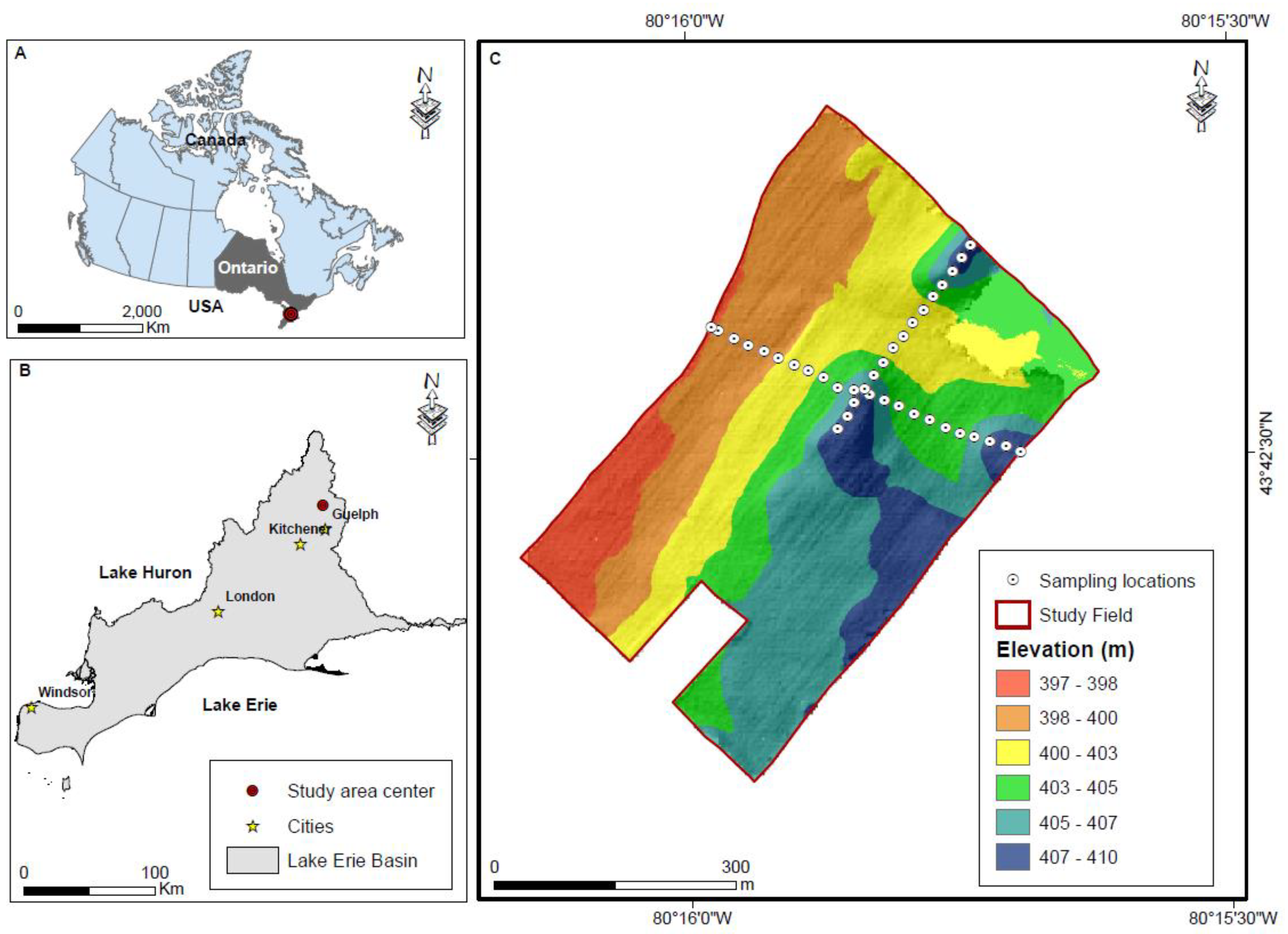
2.1. Study Site Description

The study site is located on in the Canadian Lake Erie basin of southwestern Ontario, more specifically in Wellington County (43°42′29.22″N, 80°15′54.52″W; Figure 1). The investigated site represents conventionally cultivated farmland with corn (Zea mays), soybean (Glycine max), and winter wheat (Triticum aestivum) as the dominant crops grown in a 4-year crop rotation. The topography is generally characterized by a combination of irregular moderately sloping terrains, interspersed with steep depressions (Figure 1C); soils range in texture from loam to sand (i.e., belongs to the Hillsburg fine sandy loam series). The climate is characterized by long moderate winters (November–April) and warm humid summers. The mean annual temperature is 6.7 °C and total annual precipitation is 946 mm. About one-third of the annual precipitation falls during the peak vegetative growth period, between early May and August. December, January, and February are the coldest months with a mean temperature of −3.1 °C; while June, July, and August are the warmest months with a mean temperature of 18.8 °C (Environment Canada [25]; these data are from the 1981 to 2010 Canadian Climate Normals for the Fergus Shand Dam weather station, which is located 5 km northwest of the study site).
To determine where in the field site soils should be sampled, specific terrain attributes (i.e., slope, aspect, plan curvature, profile curvature, topographic wetness, and position indices) were derived from a 2-m digital elevation model (DEM) (Land Information Ontario (LIO) data warehouse). These terrain attributes were used in an ArcGIS Clustering Analysis tool to identify statistically significant spatial clusters of high values (hot spots) and low values (cold spots) and identified the optimal location for soil sampling transects. Two transects were established to represent relevant topographic features across the field, as shown in Figure 1C. GPS coordinates were used to locate two endpoints along each transect, and the positions of the sampling locations were recorded.

2.2. Soil Samples Collection, Preparation, and Soil Total Carbon Content Measurements

Soil samples were collected along each transect at a 20-m interval (for a total of 37 locations) in spring 2017. At each location we established a 1-m equilateral triangle configuration, then three replicates were sampled per location from the topsoil horizon (0–15 cm). Soil samples were air-dried, ground, sieved over a 200-µm sieve, and analyzed for total carbon via combustion in a Leco CR-12 Carbon analyzer (Leco Corporation, St. Joseph, MI, USA) [26]. In total, 111 samples (37 × 3 replicates) were analyzed for total carbon (referred to henceforward as SOC for simplification).

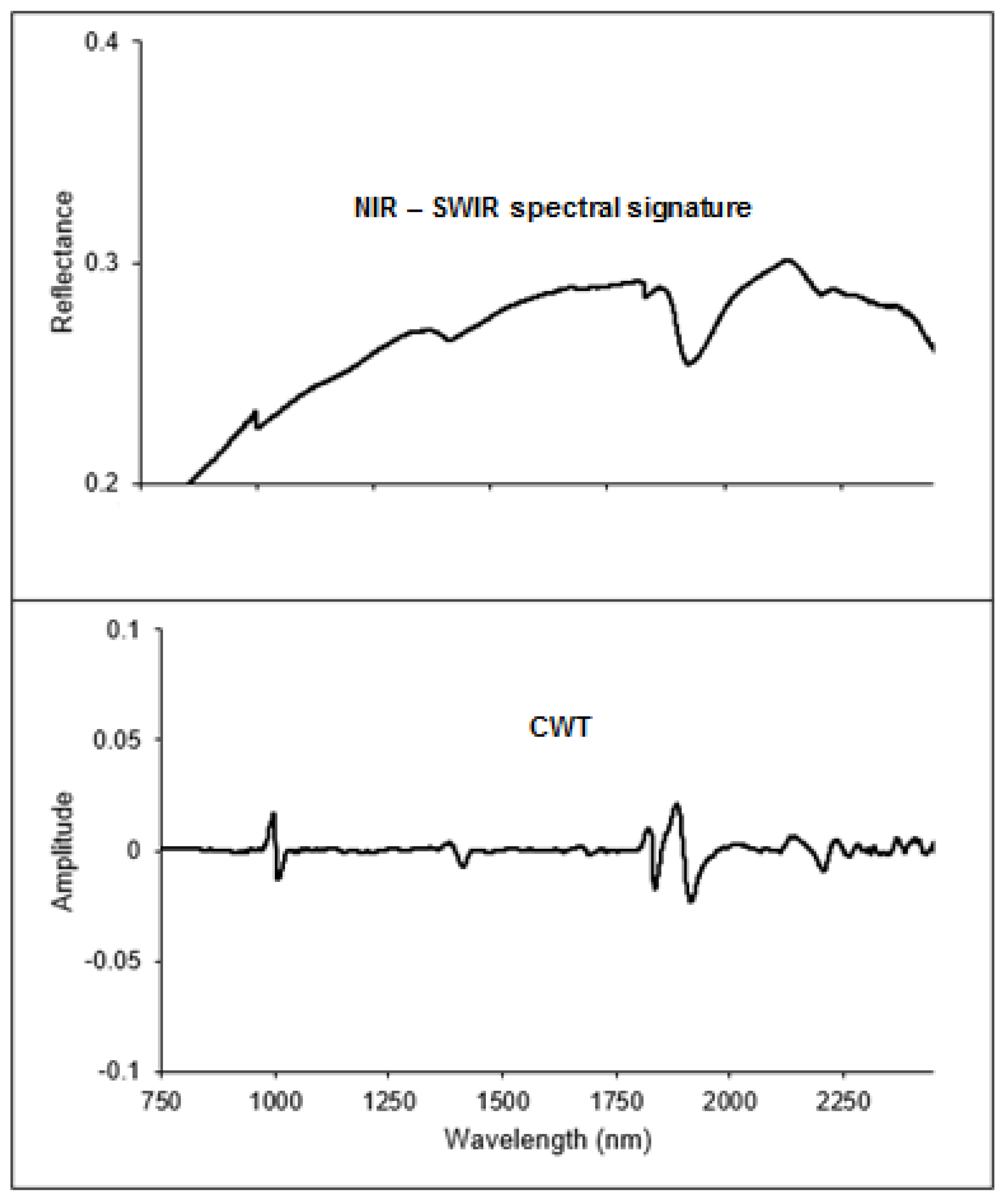
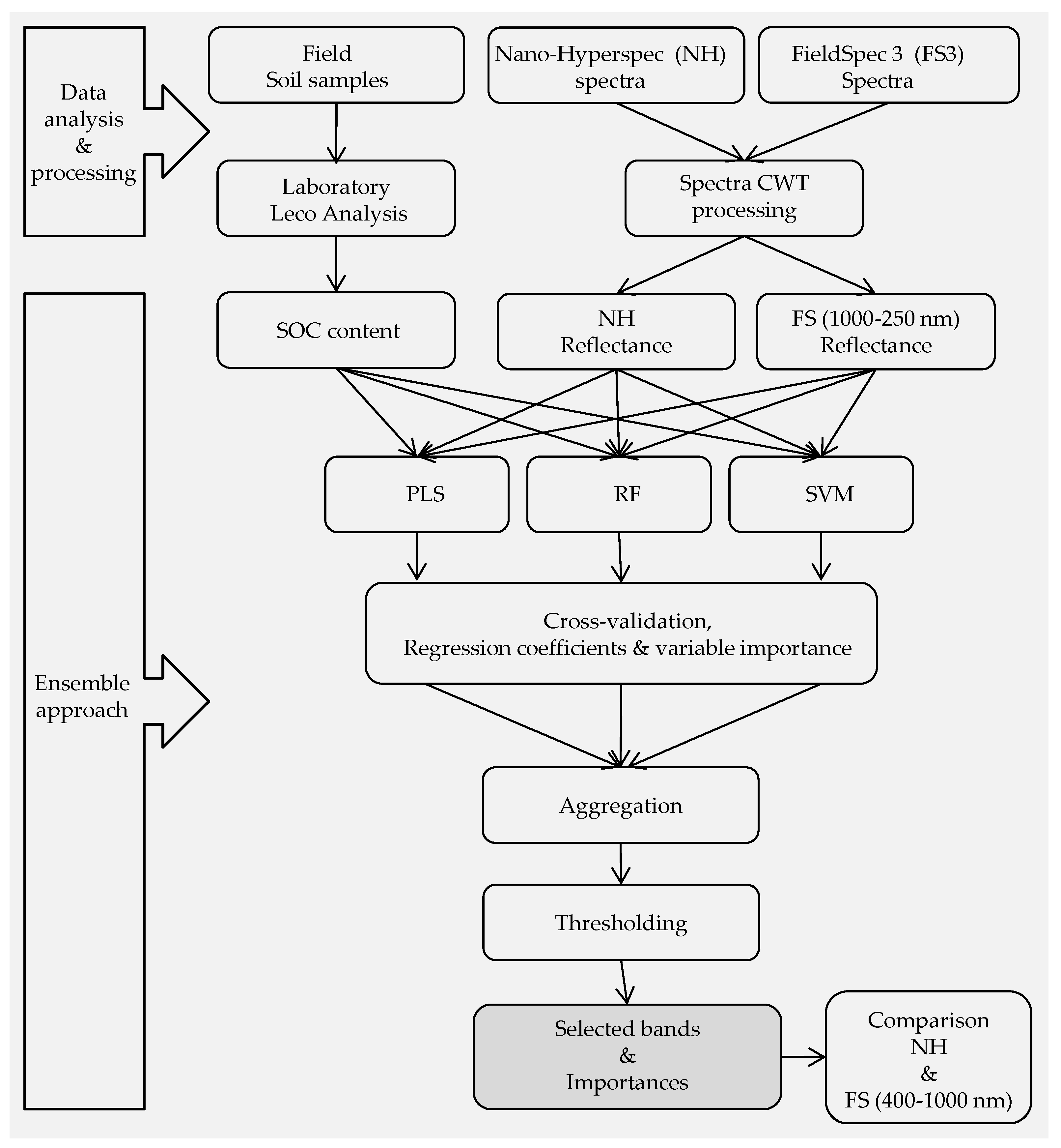
2.3. Spectral Measurements and Analysis

To determine the spectral signature of each of the 111 soil samples, spectral measurements from five locations were extracted and averaged to represent that specific sample. Reflectance spectra were obtained by determining the ratio of data acquired from a sample to data acquired for a ninety-percent-reflectance spectralon white panel (Labsphere Inc., North Sutton, NH, USA) under the same illumination conditions. All reflectance measurements were taken from flat surfaces of soil under field conditions using an unmanned aerial vehicle (UAV) airborne Nano-Hyperspec sensor (Headwall Photonics Company). This sensor was developed for deployment on UAV platforms. The Nano-Hyperspec imaging sensor provides coverage from 400–1000 nm (VNIR range). The sensor features 270 high-spectral-resolution bands with a resolution of 6 nm and 640 spatial bands. Images were captured on sunny clear-sky days at 11:30 at 1 m above the soil samples and an average spectrum of each hyperspectral image was computed. This initial 1 m assessment step aims to help to find relevant bands before doing the same process using UAVs at higher heights (i.e., 50 m).
Since the 1000–2500 nm range (NIR and SWIR) is expected to have important spectral features associated with organic carbon [27,28] and this complete range is not covered by the Nano-Hyperspec imaging sensor, we used a spectroradiometer sensor FieldSpec 3 (Analytical Spectral Devices Inc.) to collect spectral data in the 1000–2500 nm region from the 111 samples. FieldSpec 3 has three detectors and covers a wider spectral range (350–2500 nm) with a band resolution (width) of 3 nm wide in the VNIR, and 10 nm in SWIR. Samples were illuminated using a tungsten–halogen 50 W lamp positioned normal to the surface at a distance of 50 cm, thereby minimizing shadows. The fiber optic cable of the FieldSpec 3 receiving the reflected light was positioned at an angle of 35 degrees from the normal to the surface at a distance of 7 cm from the surface of the soil sample. Under these conditions, the footprint of the field of view on the measured surface was approximatively 4.5 cm in diameter. Reflectance measurements from each individual sample were recorded as an average of five scans, with a white reference sample used after every five samples.
Various studies have shown that the application of an advanced signal preprocessing transformation (i.e., first and second derivatives, continuous wavelet transform (CWT)) can improve the spectral bands selection [29] and the prediction of different soil properties [28]. To ease and improve the selection of bands related to SOC content and to fully exploit the spectral signal, each original spectrum has undergone a CWT using the R-wmtsa package [30] in R [31]. The CWT outputs were calculated for each spectral range using an eight-scale second order Gaussian transform. The specific wavelet scales 2 and 3 were selected for this study as this configuration was found to best capture the spectral features related to SOC [27]. An advantage of the CWT is its ability to be directly comparable to the original spectra. Figure 2 shows an example of the CWT for one of the samples. More details of the CWT are presented in Sorenson et al. [27].

2.4. Model Development and Evaluation

Each band of the investigated wavelengths ranges (400–1000 nm and 1000–2500 nm) was used separately in the model development. We used a multimethod ensemble modeling approach to quantify the relationship between SOC and the corresponding spectral reflectance measured at the field-level in R (R Core Team 2016). This ensemble consisted of three multivariate regression techniques, random forest regression (RF; [32]), support vector machine regression (SVM; [33]), and partial least squares (PLS; [34]) models and were used to conduct band selections and to assess the validity of the selected bands. We selected these three regression techniques because of their ability and suitability for the selection and importance ranking of bands, and their robustness when used in parallel [18]. For this multimethod ensemble strategy, the three models (i.e., RF, PLS, and SVM) were used in parallel and each of them provided statistical output values (i.e., regression coefficient and variable importance) designating the most important spectral bands for SOC prediction. The generated band importance values were merged and converted to an ensemble assessment. Bands with high influence in all three models gained a high ensemble importance and were considered important. The product of the three weighted importance values per band was taken as the ensemble importance; however, a band must be considered important by all three methods (i.e., RF, PLS, and SVM) to enter the ensemble. For the PLS model, the number of latent vectors that resulted in the smallest root mean squared error in cross-validation was used for the model to minimize the risk of over fitting. For the SVM, we used a radial basis function kernel. In this study, the fit of the model was quantified as R2 in 10-fold cross-validation for the PLS and SVM models, and as out-of-the bag error (i.e., random samples not used for building the trees) for the RF model. Detailed information about the ensemble method and the used parameters in the present study are available in Reference [18]. We first ran the ensemble model with all available spectral bands in a single analysis from each dataset (Nano-Hyperspec (400–1000 nm) and spectroradiometer (1000–2500 nm) sensors) and secondly, we further refined the band regions and re-ran the model with a set of optimal bands. The ensemble method was applied using the randomForest [35], pls [36], and e1071 [37] packages in R. The flowchart in Figure 3 provides an overview of the methodology.

3. Results

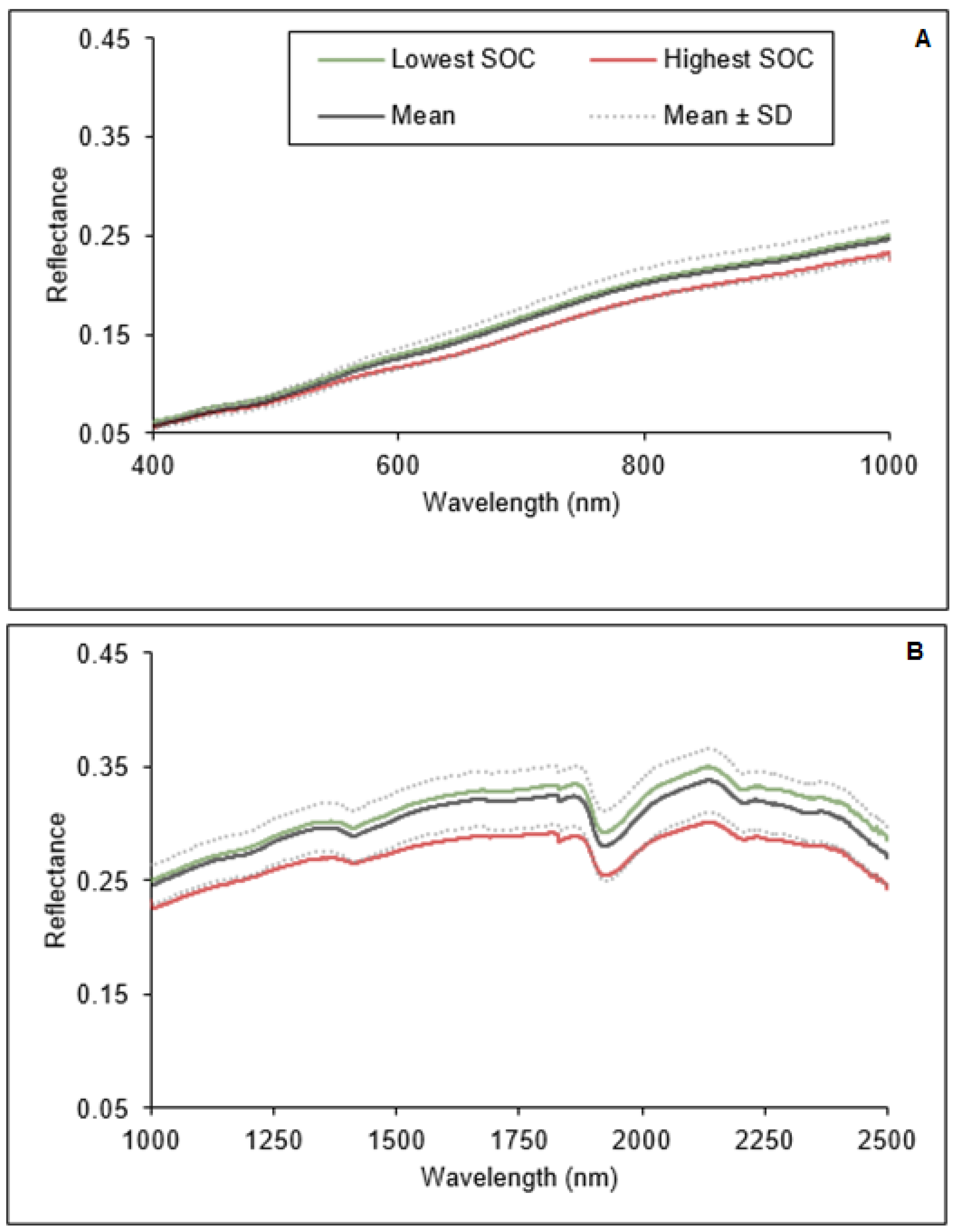
3.1. Soil Organic Carbon and Spectral Properties

Over the 111 samples, the SOC content varied from 1.60 to 4.35% with an average value of 2.32% and a standard deviation (SD) of ±0.6%, and showed a positive skewed distribution (1.36). This range of SOC values is typical of the agricultural soils in southern Ontario. Figure 4 shows the average, minimum, maximum, and mean ± SD spectrum values of the corresponding SOC for both datasets, Nano-Hyperspec and FieldSpec 3. The spectra of samples with higher SOC content have lower reflectance than samples with the lowest SOC content (Figure 4). This is consistent with previous studies that reported soil reflectance negatively correlated with SOC [38]. The overall shape of the VNIR (400–1000 nm) and NIR-SWIR (1000–2500 nm) spectra was generally similar across all samples. The VNIR region displays notable steep slope (Figure 4A) where SOC absorption in the VNIR is weak and not readily apparent, most likely because of the relatively low SOC content in our soil samples. Previous studies reported the VNIR region can relate better to soil organic matter than NIR [3] and higher precision can be achieved for agricultural soils by including the visible region [39,40]. Unlike the VNIR, the NIR-SWIR region shows very strong and distinctive features, absorptions, and peaks (Figure 4B). Some well-recognized absorption bands of water at 1400, 1950, and 2200 nm [30] are characteristic of soil and detectable across all spectra from this study.

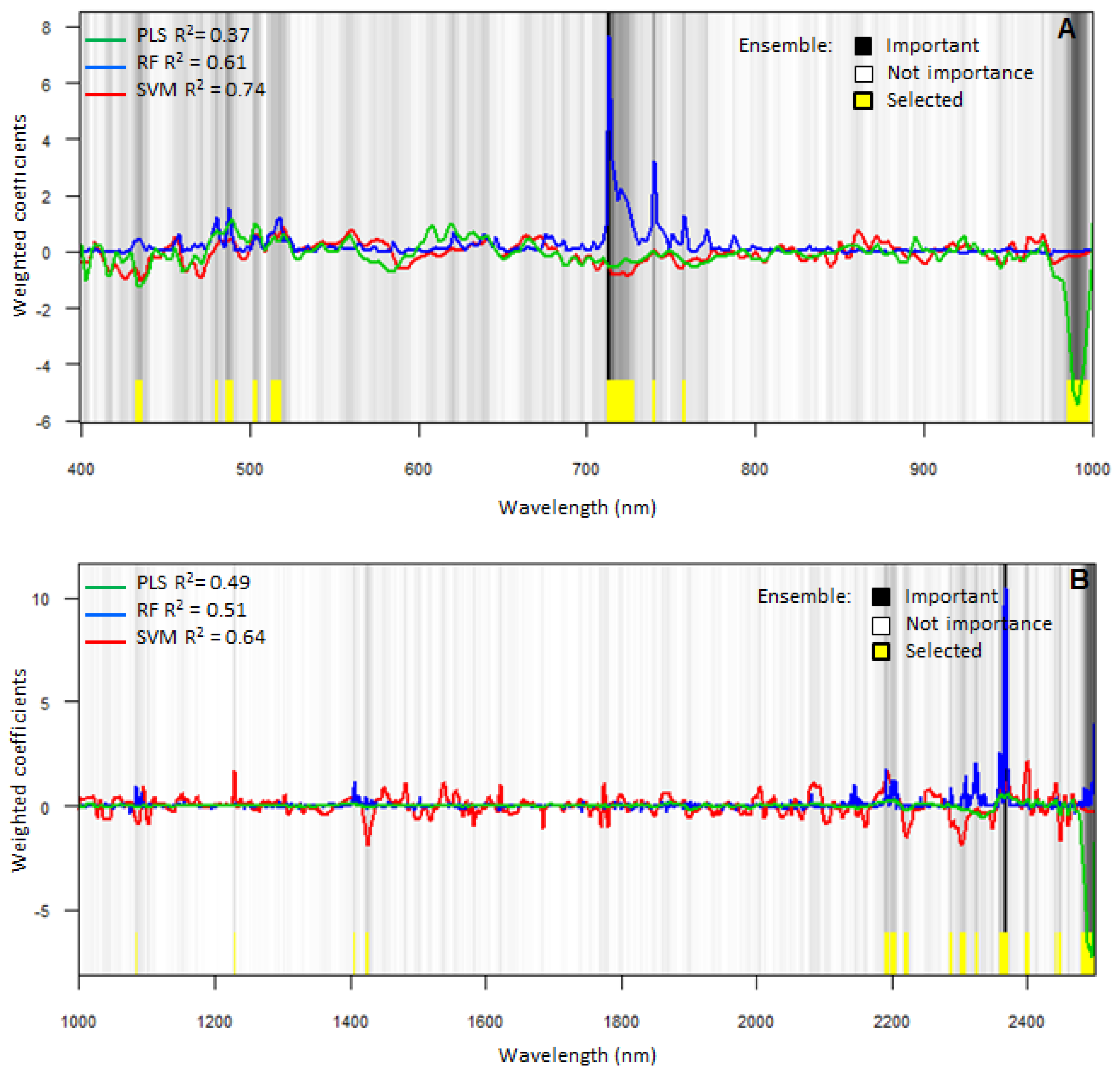
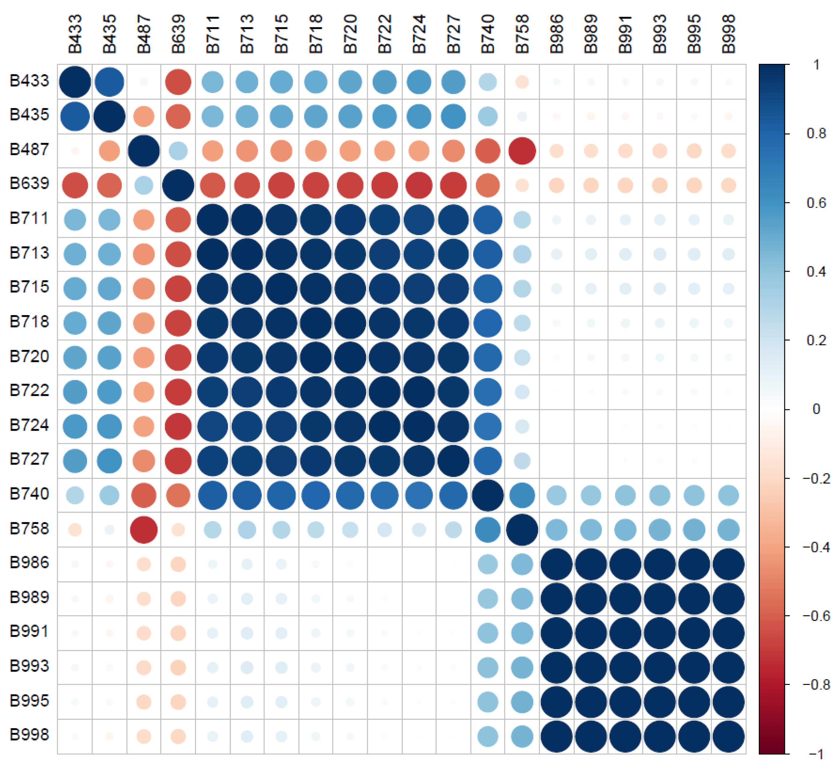
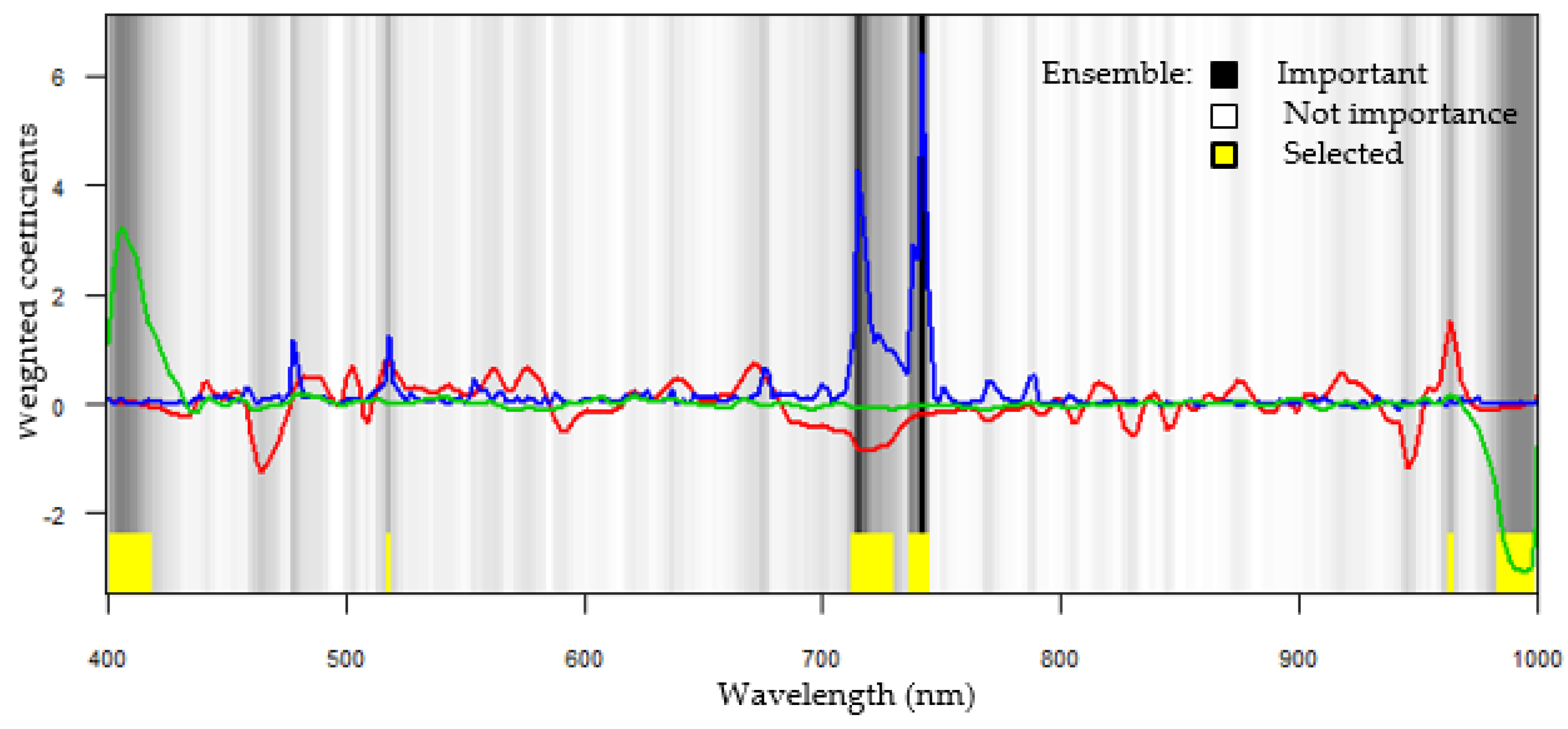
3.2. Evaluation of the Performance of the Models and Band Selection

For the Nano-Hyperspec’s spectra dataset, the model fits (i.e., R2) achieved within the ensemble model are listed in Table 1 and Figure 5. The PLS model showed the lowest R2 of 0.37, whereas SVM models showed the highest R2 of 0.74. The RF models displayed a moderate R2 of 0.62. For the spectral range 1000–2500 nm FieldSpec 3 dataset, modeled SOC resulted in a lower R2 for the RF (R2 = 0.51) and SVM (R2 = 0.64) models and a higher R2 (i.e., 0.49) observed for the PLS-based models.
Table 1 and Figure 5 display the spectral bands or regions that were selected by the ensemble modeling approach over the investigated two wavelength ranges. The ensemble modeling approach was able to identify various spectral bands throughout the VIS, NIR, and SWIR range that are sensitive to SOC. For the Nano-Hyperspec’s measured spectra, the ensemble method selected ten bands or regions at 433–435, 487, 639, 711–715, 718-727, 740, 758, and 986–998 nm. The bands that achieved the highest respective importance values were 711–715 nm and 986–998 nm. For the FieldSpec-3-measured spectra, the ensemble method selected a higher number of bands (Table 1) likely due to the finer resolution of the FieldSpec 3, as the instrument’s software interpolates over a finer sampling interval, estimating a reflectance reading every 1 nm for a total of 1501 contiguous bands. The most important bands selected were in three respective regions, 2365–2373 nm, 2481–2500 nm, and 2198–2206 nm.

3.3. Evaluation of the Performance of the Model Built Using the Subset of the Selected Bands

Once we identified the subset of bands selected by the ensemble approach (Table 1), we evaluated the performance of the individual three models (RF, PLS, and SVM) by using the subset of the selected bands. For the Nano-Hyperspec data, similar model fits were achieved for RF, PLS, and SVM models with a R2 values of 0.62, 0.39, and 0.74, respectively. Relatively higher fits were modeled using the FieldSpec 3 with R2 values of 0.55, 0.54, and 0.68, respectively.

4. Discussion

We have demonstrated that a multimethod ensemble strategy using three methods (i.e., PLS, RF, and SVM) could be a valuable selection method of spectral bands sensitive to SOC content. Our finding is consistent with previous studies (i.e., References [18,41]) that reported the ability and suitability of a multimethod ensemble for the identification, selection, and ranking of spectral bands for different remote sensing applications. There were notable differences in the model fits in the three models (i.e., PLS, RF, and SVM) included in the ensemble. The SVM model achieved the highest model fits; whereas PLS resulted in the lowest fits along the two datasets ranges (400–1000 nm and 1000–2500 nm). The RF and SVM model fits in our study are similar to those obtained in a very recent study [15] (0.62 vs 0.63 and 0.74 vs 0.73, respectively); our PLS fit was substantially lower (0.37 vs 0.67). This lower fit can be due to more data (i.e., 8426 samples) used in Tsakiridis et al.’s study [15] or by the sensitivity of PLSR, being a parametric regression technique, towards a skewed distribution of the SOC contents [42]. In light of these results, the SVM model seems to have a superior influence on the ensemble selection than RF and PLS models, based on the initial weighting calculation of the importance value within the ensemble. For a band to be retained in the ensemble, all the three methods needed to agree on its selection. This multiple aggregation of variable importance values for band selection balanced the effect of singular strong and weak models. The agreement among the three methods underlines the general importance of band and region in its relation to SOC content and eliminates unnecessary information that might otherwise be included if only one model is considered. Overall, the results of the multimethod ensemble for the identification and selection of related SOC hyperspectral bands were good, though additional work will be needed to investigate the inclusion suitability of additional methods (i.e., neutral networks, cubist, and principal component regression) in the ensemble that can improve the model fits.
We applied cross-validation which uses a test set (i.e., data not seen by the model) to evaluate model performance. Cross-validation has proven to be a robust method for modeling SOC, especially with machine learning methods (i.e., RF and SVM). Nevertheless, we compared our cross-validation-based model performance with an independent dataset of soil samples. This was done by randomly splitting the dataset (n = 111) into a training dataset (three-quarter of the total soil samples) and a validation dataset (one-quarter); the models were built using the training dataset from which the important bands band were extracted; applied the three models on the validation dataset; quantified the model fits; and used these as weights in the ensemble selection. Table 2 shows that the R2 values obtained for the validation are close to those obtained during the training and the cross-validation, confirming the stability of the ensemble model used in this study. It should also be noted that the R2 accuracies obtained here by the cross-validation are similar to those obtained with additional accuracy assessment indices (i.e., root mean square error (RMSE) and ratio of performance to deviation (RPD); Table 2); suggesting that R2 is sufficiently robust to explain the models. The RPD values (RPD > 1.4 [39]) for the RF and MVS models indicate that these two models are good predictors compared to the PLS model for both datasets (i.e., the FieldSpec 3 and Nano-Hyperspec), which is consistent with the findings of this study.
We identified a relevant subset of bands in the visible, NIR, and SWIR that are of interest in SOC quantification and mapping. The most important identified bands or regions were 711–715, 727, 986–998, 433–435, 2365–2373, 2481–2500, and 2198–2206 nm. Some of the selected bands are in accordance with other studies that identified important bands (or wavelengths) using a single modeling approach (i.e., PLS regression) for predicting total carbon in the first 15 cm of soil, whereas other selected bands are new and specific to this study. For instance, Sarkhot et al. [40] identified wavelengths 358, 378–438, 498–768, 728–1148, 1208–1788, 1868, 1888–2258, 2278–2338, 2358–2448, 2468–2488 nm as important wavelengths for estimation of total carbon in the soil. In our case, the number of selected bands and range of band regions are significantly lower than those obtained by Sarkhot et al. [40], most probably because our ensemble method was more selective, than the single modeling approach. It is important to mention that the correlation between the selected band subset was not considered a priori during the selection procedure, leading to the situation where the collinearity among the selected bands is still relatively high (Figure 6).
It is well established in the literature that the position of diagnostic bands is related to the mineral composition of the soil itself [7]; and does not vary with factors such as texture (i.e., particle size fraction) or moisture (soil water content). For example, Rienzi et al. [43] reported that soil moisture had a relatively small impact on the relative importance of bands used in estimates of organic carbon in soil. Nevertheless, the authors also found that their model predictions were better for air-dried soil samples, the material used in this study. Previous studies also found that the only spectra parameters that vary with texture are the overall brightness and the amplitude of features (i.e., absorption bands and peaks) [5].
It is important to mention that the most important identified bands related to SOC in the SWIR (i.e., 2481–2500 nm) are different from diagnostic absorption bands of carbonate minerals (e.g., calcite or dolomite; [44,45] usually cited as an indicator of inorganic carbon input in soil). In addition, it is well known that organic carbon in soil can mask or even suppress carbonate bands [44]; thus, this helps in associating the selected bands here to SOC with no overlap with carbonate. Even though, the VNIR FieldSpec 3 data were not the focus of this study, for the assessment of the validity of the selected bands, the reflectance spectra data from FieldSpec 3 along the 400–1000 nm region were resampled and compared to the spectral resolution of the Nano-Hyperspec. Overall, the resulting selected bands that achieved the highest respective importance (i.e., 713–744 nm and 984–998 nm; Figure 7) are located at very similar wavelengths regions compared to the Nano-Hyperspec sensor sensors (Figure 5A).
This similarity of the selected bands by both instrument bands suggests that the selected bands may represent robust diagnostic bands for estimation of SOC content and that the ensemble model can be relatively stable within the range of SOC variability common in many agricultural soils in southern Ontario and allow for the use of sensors, such as the Nano for SOC mapping, and may reinforce the development of digital soil mapping. In addition, the final models that were built using the selected subset of bands by the ensemble overall outperforms the initial models including the full spectral data set; this supports the robustness of the band selection. Therefore, the selected optimal bands in this study can be used to improve predictive accuracies. In addition, identification of the most sensitive bands for SOC is of interest to develop optimal sensors equipped with only a few bands. For instance, the set of the identified bands could be of great importance for the UAV industry because it would greatly help in creating new well-optimized SOC specific sensors. Beyond the selected bands here for SOC, it would be interesting to apply the multimethod modeling approach to selected sensitive bands to additional subtle soil proprieties such as total nitrogen content. This would greatly facilitate SOC and nitrogen (N) inventory and assessment of spatial and temporal changes at a field scale, following changes in land use and/or management practices.

5. Conclusions

In this study, we showed that a band analysis conducted on two hyperspectral regions (400–1000 nm and 1000–2500 nm) using an ensemble approach of three methods (PLS, RF, and SVM) was able to identify specific spectral bands or regions that contain relevant information for SOC content assessment. We believe that the ensemble modeling approach is a robust promising method for the quantitative analysis for spectral data in VNIR and SWIR in relation to SOC content. The hyperspectral bands selected by the ensemble approach can subsequently be used (1) as preselection to build predictive models from new data sets, and (2) for the development of new well-optimized SOC specific sensors to be mounted on UAVs. In our future studies, these bands or regions analyses coupled with UAV-derived hyperspectral imagery, acquired at an optimal height, will be validated with spatially dense grid sampling design over the same field. This approach is expected to confirm relationships between specific spectral bands or regions and SOC at a larger scale (i.e., field scale) and to account for high spatial variability. The use of UAV technology with the new generation of multispectral and hyperspectral sensors could allow the assessment of the continuous spatial and temporal variability of SOC, among other topsoil properties, at relatively low costs and higher resolution (i.e., submetric). Compared to field soil sampling, satellite and aerial surveys, UAV-sensing is expecting to show many advantages in terms of cost, flexibility, and spatial and temporal resolution. These advantages will make UAV-sensing an attractive solution for scientific studies, particularly where high continuous spatial resolution data are needed.

Author Contributions

A.L., A.A.B., P.V. and R.C.M. conceived and designed the field experiments. A.L. and L.B. participated in the soil samples collection. L.B. conducted the laboratory soil organic carbon analyses. H.F. conceived and wrote the initial coding for the ensemble method and worked with L.B. to adapt the method for this study. M.M., Y.H. and P.D.D. from the University of Toronto were closely involved in the acquisition, and the processing of the FieldSpec 3 data in their lab. A.L. analyzed and interpreted the data with the participation of all the authors. A.L. wrote the original manuscript and has been designated responsible for handling correspondence at all stages of refereeing and publication. A.A.B., P.V. and R.C.M. contributed to the finding acquisition and R.C.M. is the PI and responsible for the project management. All the authors have contributed substantially to revising the submitted manuscript.

Funding

The authors gratefully acknowledge funding from Agricultural Greenhouse Gases Program-Agriculture and Agri-Food Canada (AGGP-015 awards to Dr. Ralph Martin), the Christian Farmers Federation of Ontario, and the Canada First Excellence Research Fund: Food from Thought.

Acknowledgments

The authors thank Woodrill Ltd. for access to their land for this study, Alexander McLaren, Renato Pardo Lara, and many students from the University of Guelph who assisted with fieldwork, acquisition and processing of the data. (e.g., materials used for experiments). We also thank the editor, managing editor, and four anonymous reviewers for their constructive comments.

Conflicts of Interest

The authors declare no conflicts of interest.

References

  1. Lal, R. Soil Carbon Sequestration Impacts on Global Climate Change and Food Security. Science 2004, 304, 1623–1627. [Google Scholar] [CrossRef] [Green Version]
  2. Goidts, E.; Van Wesemael, B. Regional assessment of soil organic carbon changes under agriculture in Southern Belgium (1955–2005). Geoderma 2007, 141, 341–354. [Google Scholar] [CrossRef]
  3. Weng, L. 2016 & 2011 Census of Agriculture and Strategic Policy Branch, OMAFRA. 2017. Available online: http://www.omafra.gov.on.ca/english/stats/county/southern_ontario.htm (accessed on 13 May 2019).
  4. Ben-Dor, E.; Banin, A. Near-infrared analysis as a rapid method to simultaneously evaluate several soil properties. Soil. Sci. Soc. Am. J. 1995, 44, 364–372. [Google Scholar] [CrossRef]
  5. Stenberg, B.; Rossel, R.A.V.; Mouazen, A.M.; Wetterlind, J. Visible and near infrared spectroscopy in soil science. Adv. Agron. 2010, 107, 163–215. [Google Scholar]
  6. Angelopoulou, T.; Tziolas, N.; Balafoutis, A.; Zalidis, G.; Bochtis, D. Remote Sensing Techniques for Soil Organic Carbon Estimation: A Review. Remote Sens. 2019, 11, 676. [Google Scholar] [CrossRef]
  7. Nocita, M.; Stevens, A.; van Wesemael, B.; Aitkenhead, M.; Bachmann, M.; Barthès, B.; Ben Dor, E.; Brown, D.J.; Clairotte, M.; Csorba, A.; et al. Soil Spectroscopy: An Alternative to Wet Chemistry for Soil Monitoring. Adv. Agron. 2015, 132, 139–159. [Google Scholar]
  8. Crucil, G.; Castaldi, F.; Aldana-Jague, E.; van Wesemael, B.; Macdonald, A.; Van Oost, K. Assessing the Performance of UAS-Compatible Multispectral and Hyperspectral Sensors for Soil Organic Carbon Prediction. Sustainability 2019, 11, 1889. [Google Scholar] [CrossRef]
  9. Verrelst, J.; Rivera, J.P.; Gitelson, A.; Delegido, J.; Moreno, J.; Camps-Valls, G. Spectral band selection for vegetation properties retrieval using Gaussian processes regression. Int. J. Appl. Earth Obs. 2016, 52, 554–567. [Google Scholar] [CrossRef]
  10. Li, S.; Qiu, J.; Yang, X.; Liu, H.; Wan, D.; Zhu, Y. A novel approach to hyperspectral band selection based on spectral shape similarity analysis and fast branch and bound search. Eng. Appl. Artif. Intel. 2014, 27, 241–250. [Google Scholar] [CrossRef] [Green Version]
  11. Li, S.; Zheng, Z.; Wang, Y.; Chang, C.; Yu, Y. A new hyperspectral band selection and classification framework based on combining multiple classifiers. Pattern Recogn. Lett. 2016, 83, 152–159. [Google Scholar] [CrossRef]
  12. Ben-Dor, E.; Chabrillat, S.; Demattê, J.; Taylor, G.; Hill, J.; Whiting, M.; Sommer, S. Using Imaging Spectroscopy to study soil properties. Remote Sens. Environ. 2009, 113, S38–S55. [Google Scholar] [CrossRef]
  13. Stevens, A.; Udelhoven, T.; Denis, A.; Tychon, B.; Lioy, R.; Hoffmann, L.; Van Wesemael, B. Measuring soil organic carbon in croplands at regional scale using airborne imaging spectroscopy. Geoderma 2010, 158, 32–45. [Google Scholar] [CrossRef]
  14. Gomez, C.; Viscarra, R.A.; Mcbratney, A.B. Soil organic carbon prediction by hyperspectral remote sensing and fi eld vis-NIR spectroscopy: An Australian case study. Geoderma 2008, 146, 403–411. [Google Scholar] [CrossRef]
  15. Tsakiridis, U.L.; Theocharis, J.B.; Ben-Dor, E.; Zalidis, G.C. Using interpretable fuzzy rule-based models for the estimation of soil organic carbon from VNIR/SWIR spectra and soil texture. Chemom. Intell. Lab. Syst. 2019, 189, 39–55. [Google Scholar] [CrossRef]
  16. Deng, F.; Minasny, B.; Knadel, M.; McBratney, A.; Heckrath, G.; Greve, M.H. Using vis-NIR spectroscopy for monitoring temporal changes in soil organic carbon. Soil Sci. 2013, 178, 389–399. [Google Scholar] [CrossRef]
  17. Schillaci, C.; Lombardo, L.; Saia, S.; Fantappiè, M.; Märker, M.; Acutis, M. Modelling the topsoil carbon stock of agricultural lands with the Stochastic Gradient Treeboost in a semi-arid Mediterranean region. Geoderma 2017, 286, 35–45. [Google Scholar] [CrossRef]
  18. Feilhauer, H.; Asner, G.P.; Martin, R.E. Multi-method ensemble selection of spectral bands related to leaf biochemistry. Remote Sens. Environ. 2015, 164, 57–65. [Google Scholar] [CrossRef]
  19. Genuer, R.; Poggi, J.-M.; Tuleau-Malot, C. Variable selection using random forests. Pattern Recogn. Lett. 2010, 31, 2225–2236. [Google Scholar] [CrossRef] [Green Version]
  20. Xie, H.; Yang, X.; Drury, C.; Yang, J.; Zhang, X. Predicting soil organic carbon and total nitrogen using mid-and near-infrared spectra for Brookston clay loam soil in Southwestern Ontario, Canada. Can. J. Soil Sci. 2011, 91, 53–63. [Google Scholar] [CrossRef]
  21. Zhang, L.; Yang, X.M.; Drury, C.; Chantigny, M.; Gregorich, E.; Miller, J.; Bittman, S.; Reynolds, D.; Yang, J.Y. Infrared spectroscopy prediction of organic carbon and total nitrogen in soil and particulate organic matter from diverse Canadian agricultural regions. Soil Sci. Soc. Am. J. 2018, 98, 77–90. [Google Scholar] [CrossRef]
  22. Blackburn, G.A. Hyperspectral remote sensing of plant pigments. J. Exp. Bot. 2006, 58, 855–867. [Google Scholar] [CrossRef] [Green Version]
  23. Ustin, S.L.; Gitelson, A.A.; Jacquemoud, S.; Schaepman, M.; Asner, G.P.; Gamon, J.A.; Zarco-Tejada, P. Retrieval of foliar information about plant pigment systems from high resolution spectroscopy. Remote Sens. Environ. 2009, 113, S67–S77. [Google Scholar] [CrossRef] [Green Version]
  24. Liu, Y.; Jiang, Q.; Fei, T.; Wang, J.; Shi, T.; Guo, K.; Li, X.; Chen, Y. Transferability of a Visible and Near-Infrared Model for Soil Organic Matter Estimation in Riparian Landscapes. Remote Sens. 2014, 6, 4305–4322. [Google Scholar] [CrossRef] [Green Version]
  25. Environment Canada. Canadian Climate Normals 1981–2010: Fergus Shand Dam Weather Station. 2011. Available online: http://climate.weather.gc.ca/climate_normals/index_e.html (accessed on 13 May 2019).
  26. Wang, D.; Anderson, D.W. Direct measurement of organic carbon content in soils by the Leco CR-12 carbon analyzer. Commun. Soil Sci Plan. 1998, 29, 15–21. [Google Scholar] [CrossRef]
  27. Sorenson, P.; Small, C.; Tappert, M.; Quideau, S.; Drozdowski, B.; Underwood, A.; Janz, A. Monitoring organic carbon, total nitrogen, and pH for reclaimed soils using field reflectance spectroscopy. Can. J. Soil Sci. 2017, 97, 241–248. [Google Scholar] [CrossRef]
  28. Viscarra Rossel, R.; Behrens, T. Using data mining to model and interpret soil diffuse reflectance spectra. Geoderma 2010, 158, 46–54. [Google Scholar] [CrossRef]
  29. Schlerf, M.; Atzberger, C.; Hill, J.; Buddenbaum, H.; Werner, W.; Schüler, G. Retrieval of chlorophyll and nitrogen in Norway spruce (Picea abies L. Karst.) using imaging spectroscopy. Int. J. Appl. Earth Obs. 2010, 12, 17–26. [Google Scholar] [CrossRef]
  30. Constantine, W.; Percival, D. Wavelet Methods for Time Series Analysis. 2017. Available online: https://cran.r-project.org/package=wmtsa (accessed on 29 May 2019).
  31. R Core Team R: A Language and Environment for Statistical Computing; R Foundation for Statistical Computing: Vienna, Austria, 2019.
  32. Breiman, L. Random forests. Mach. Learn. 2001, 45, 5–32. [Google Scholar] [CrossRef]
  33. Karatzoglou, A.; Smola, A.; Hornik, K.; Zeileis, A. kernlab-an S4 package for kernel methods in R. J. Stat. Softw. 2004, 11, 1–20. [Google Scholar] [CrossRef]
  34. Mevik, B.-H.; Wehrens, R. Introduction to the pls Package. In Help Section of The “Pls” Package of R Studio Software; R Foundation for Statistical Computing: Vienna, Austria, 2015; pp. 1–23. [Google Scholar]
  35. Liaw, A.; Wiener, M. Classification and regression by random Forest. R News 2002, 2, 18–22. [Google Scholar]
  36. Mevik, B.-H.; Wehrens, R.; Liland, K.H. Pls: Partial Least Squares and Principal Component Regression; R Package Version 2.4-3; R Foundation for Statistical Computing: Vienna, Austria, 2018. [Google Scholar]
  37. Meyer, D.; Dimitriadou, E.; Hornik, K.; Weingessel, A.; Leisch, F.; Chang, C.-C.; Lin, C.-C. e1071: Misc Functions of the Department of Statistics (e1071), R package version 1.7-0.1; TU Wien: Vienna, Austria, 2019. [Google Scholar]
  38. Conforti, M.; Castrignanò, A.; Robustelli, G.; Scarciglia, F.; Stelluti, M.; Buttafuoco, G. Laboratory-based Vis-NIR spectroscopy and partial least square regression with spatially correlated errors for predicting spatial variation of soil organic matter content. Catena 2015, 124, 60–67. [Google Scholar] [CrossRef]
  39. Chang, C.-W.; Laird, D.A.; Mausbach, M.J.; Hurburgh, C.R. Near-infrared reflectance spectroscopy-principal components regression analyses of soil properties. Soil Sci. Soc. Am. J. 2001, 65, 480–490. [Google Scholar] [CrossRef]
  40. Sarkhot, D.; Grunwald, S.; Ge, Y.; Morgan, C. Comparison and detection of total and available soil carbon fractions using visible/near infrared diffuse reflectance spectroscopy. Geoderma 2011, 164, 22–32. [Google Scholar] [CrossRef]
  41. Du, P.; Xia, J.; Zhang, W.; Tan, K.; Liu, Y.; Liu, S. Multiple classifier system for remote sensing image classification: A review. Sensors 2012, 12, 4764–4792. [Google Scholar] [CrossRef]
  42. Jiang, Q.; Chen, Y.; Guo, L.; Fei, T.; Qi, K. Estimating Soil Organic Carbon of Cropland Soil at Different Levels of Soil Moisture Using VIS-NIR Spectroscopy. Remote Sens. 2016, 8, 755. [Google Scholar] [CrossRef]
  43. Rienzi, E.A.; Mijatovic, B.; Mueller, T.G.; Matocha, C.J.; Sikora, F.J.; Castrignanò, A. Prediction of soil organic carbon under varying moisture levels using reflectance spectroscopy. Soil Sci. Soc. Am. J. 2014, 78, 958–967. [Google Scholar] [CrossRef]
  44. Van der Meer, F. Spectral reflectance of carbonate mineral mixtures and bidirectional reflectance theory: Quantitative analysis techniques for application in remote sensing. Remote Sens. Rev. 1995, 13, 67–94. [Google Scholar] [CrossRef]
  45. Ben-Dor, E.; Banin, A. Near-infrared reflectance analysis of carbonate concentrations in soils. Appl. Spectrosc. 1990, 44, 1064–1069. [Google Scholar] [CrossRef]
Figure 1. Map showing the location of the study site in (A) southwestern Ontario within (B) the Lake Erie basin. (C) The 37 sample locations along transects used in this study were in an agricultural field with a topographic overview.
Remotesensing 11 01298 g001
Figure 2. Example of the near-infrared (NIR) and shortwave-infrared (SWIR) spectrum and its continuous wavelet transform (CWT) for a soil sample that represents the highest SOC content over the study area. The wavelet is a Gaussian wavelet transform. Note the peak near to 1000 nm is an artifact due to detector offset.
Remotesensing 11 01298 g002
Figure 3. Flowchart of the methodology (i.e., analyses, processing steps, and the modeling) used in this study. A detailed description of the ensemble multimethod is provided in Reference [18]. PLS: Partial least squares; RF: Random forest; SOC: Soil organic carbon; SVM: Support vector machine.
Remotesensing 11 01298 g003
Figure 4. (A) Visible near-infrared (VNIR) (400–1000 nm) and the (B) near-infrared-shortwave-infrared (NIR-SWIR) (400–1000 nm) regions showing spectra from the investigated agricultural soils samples: The average SOC of the 111 samples, soils with the highest and lowest SOC content (4.35% and 1.69%, respectively), and dashed spectra lines indicate the mean ± one standard deviation (SD). Untransformed spectra in (A) and (B) are shown for illustrations and only corresponding CWT spectra were used in the model.
Remotesensing 11 01298 g004
Figure 5. Results of the ensemble approach for the relationship between the SOC content and reflectance in the (A) VNIR and (B) NIR-SWIR regions. Black and white color range in each graph illustrates the relative importance of the respective selected bands (in yellow). PLS, RF, and SVM coefficients are measures of band importance with the ensemble and their combination determines the ensemble importance. The sign of the weighted coefficients indicates a positive or negative relationship while the absolute value of the coefficients is the variable importance. CWT spectra were used in the model.
Remotesensing 11 01298 g005
Figure 6. Pearson correlation coefficient matrix comparing paired selected band subset (i.e., B433). Positive correlations are shaded blue, whereas negative correlations are shaded red. The strength of the correlation is indicated by dot size and blue or red color saturation. High correlation between bands is also indicated by the size of the colored oval delineating each comparison.
Remotesensing 11 01298 g006
Figure 7. Results of the ensemble approach for the relationship between the SOC content and reflectance in the 400–1000 nm regions using FieldSpec 3 data. To enable comparison, the FieldSpec 3 reflectance data were resampled to the spectral range and resolution of the Nano-Hyperspec sensor. Black and white color range illustrates the relative importance of the respective selected bands (in yellow). The sign of the weighted coefficients indicates a positive or negative relationship while the absolute value of the coefficients is the variable importance. CWT spectra were used in the ensemble model to generate the bands selection.
Remotesensing 11 01298 g007
Table 1. Selected bands for the estimation of SOC using an ensemble modelling approach (PLS, RF, and SVM). R2 values are the model fits achieved within the ensemble model.
Spectra R2 Selected Bands (nm)
PLSRFSVM
VNIR0.370.610.74433–435, 487, 639, 711–715 *, 718–727, 740, 758, 986–998 *
NIR-SWIR0.490.510.641085, 1230, 1407, 1424–1428, 2082, 2189-2196, 2198–2206 2220–2224, 228–2327, 2359–2363, 2365–2373 *, 2397–2403, 2443–2451, 2481–2500 *
*: Bands that achieved the highest respective importance; VNIR and NIR-SWIR represent Nano-Hyperspec and FieldSpec 3 spectra dataset, respectively.
Table 2. Descriptive accuracy indices of the SOC from all the dataset (n = 111), training dataset (3/4), and validation dataset (1/4). RMSE: Root mean square error.
Dataset/ModelAll DataSplit Data (R2)
R2 (Cross-Validation)RMSERPDTrainingValidation
NIR-SWIR
PLS0.490.441.40.470.45
RF0.510.431.50.530.51
SVM0.640.391.60.620.60
VNIR
PLS0.370.471.30.410.35
RF0.610.381.60.640.61
SVM0.740.351.80.750.72
NIR-SWIR and VNIR represent FieldSpec 3 and Nano-Hyperspec spectra dataset, respectively. RPD = ratio of performance to deviation.

