A Gray Scale Correction Method for Side-Scan Sonar Images Based on Retinex

1
College of Automation, Harbin Engineering University, Harbin 150001, China
2
School of Management, Harbin University of Commerce, Harbin 150028, China
*
Author to whom correspondence should be addressed.
Remote Sens. 2019, 11(11), 1281; https://doi.org/10.3390/rs11111281
Submission received: 24 April 2019
/
Revised: 23 May 2019
/
Accepted: 25 May 2019
/
Published: 29 May 2019
(This article belongs to the Special Issue Radar and Sonar Imaging and Processing)
Abstract
:When side-scan sonars collect data, sonar energy attenuation, the residual of time varying gain, beam patterns, angular responses, and sonar altitude variations occur, which lead to an uneven gray level in side-scan sonar images. Therefore, gray scale correction is needed before further processing of side-scan sonar images. In this paper, we introduce the causes of gray distortion in side-scan sonar images and the commonly used optical and side-scan sonar gray scale correction methods. As existing methods cannot effectively correct distortion, we propose a simple, yet effective gray scale correction method for side-scan sonar images based on Retinex given the characteristics of side-scan sonar images. Firstly, we smooth the original image and add a constant as an illumination map. Then, we divide the original image by the illumination map to produce the reflection map. Finally, we perform element-wise multiplication between the reflection map and a constant coefficient to produce the final enhanced image. Two different schemes are used to implement our algorithm. For gray scale correction of side-scan sonar images, the proposed method is more effective than the latest similar methods based on the Retinex theory, and the proposed method is faster. Experiments prove the validity of the proposed method.
1. Introduction
With the continuous development of side-scan sonar technology, aspects of side-scan sonars, such as data acquisition stability, sonar image resolution, and image clarity have been improved, providing better technical support for hydrographic surveying and charting. Given the development of marine resource, it is necessary to scan the seabed with side-scan sonars to grasp the general information of the seabed scene and topography for many applications, such as offshore oil drilling, channel dredging, submarine pipeline detection, seabed structure detection, marine environment detection, marine archaeology, and detection and location of large-scale seabed targets [1,2,3,4].
In Figure 1, a side-scan sonar is scanning the seabed scene. The side-scan sonar transducer installed on both sides of the Autonomous Underwater Vehicle (AUV) emits spherical acoustic signals. After reflection from the seabed, the reflected signals are collected and received by the receiver according to the transmission time of the sonar signal. A side-scan sonar image is formed by converting the reflected signal intensity into the gray level. However, the energy of the sonar acoustic wave can attenuate in water. There are three main types of attenuation. The first category is physical attenuation, the second is the absorption of seawater and the third is echo attenuation [5,6,7]. In addition to the causes of sonar energy attenuation, side-scan sonar image is also affected by beam patterns, angular responses of different sediments, and changes in seabed topography [7,8,9]. Based on the above reasons, the gray-scale of side-scan sonar images is uneven.
As shown in Figure 2, the original side-scan sonar image has uneven gray distribution, which affects the interpretation of the side-scan sonar image and the subsequent image processing. Therefore, gray scale correction should be conducted before processing the side-scan sonar image, such as image matching, stitching, and target recognition [10,11,12].
2. Current Gray Scale Correction Methods for Side-Scan Sonar Images
At present, many kinds of gray scale correction methods are available for side-scan sonar images, which can be categorized into six kinds of methods.
2.1. Time Variant Gain (TVG)
The TVG method is a commonly used method for gray scale correction of side-scan sonar images. The time variant gain method, adopted by Johnson et al., is based on the distance between each point of the seabed and the sonar array in the side-scan sonar image [9,13]. The side-scan sonar images are compensated using Equation (1):
where EL is the compensation amount, TL is the energy loss caused by the propagation process, TS is the target strength, R is the propagation distance, α is the absorption coefficient, Sf is the seabed backscattering intensity. Since α and R cannot be easily obtained, their empirical values are required in the compensation. The TVG method is usually implemented using hardware. While the intensity can be compensated for, to a certain extent, it is impossible to mimic the same sonar energy attenuation process. Sometimes unrealistic gain parameters cause secondary gray distortion. Two problems arise if we use the algorithm in Equation (1) to gray correct side-scan sonar images. (1) It is difficult to determine the specific values of the parameters in Equation (1) only using side-scan sonar images, so imbalanced correction may occur. (2) Different side-scan sonar images require different parameters in the TVG equation to achieve better image enhancement, so the algorithm is not universal.
2.2. Histogram Equalization (HE)
Histogram equalization is used to improve the uniformity of the gray distribution of the side-scan sonar image by adjusting the gray distribution of the entire image. The essence of histogram equalization involves enlarging the gray level difference of the image, and the overall contrast of the image is improved after equalization. HE has been widely used because of its simplicity and directness [14]. However, HE often increases image noise, and because some gray scale merging results in blurring the weak edges of the image, it leads to over-enhancement in the regions with large histogram peaks, which is extremely disadvantageous to side-scan sonar image processing. Therefore, histogram equalization is not the best method to address gray distortion in side-scan sonar images.
2.3. Nonlinear Compensation
Nonlinear compensation involves dividing the range of 0 to 255 gray levels into many parts, and then to compensate the gray value of different parts with a piecewise function. However, this leads to excessive gray correction in side-scan sonar images, which may distort the original information of the side-scan sonar image [15].
2.4. Function Fitting
Function fitting method involves using N Ping side-scan sonar data as the selected image. Then, according to the average value of pixels in the column of the selected sonar image, the gray change curve is obtained in the row direction and it is fit with a function. Next, the image is compensated and corrected according to the function obtained by fitting. The representative methods are mixed exponential regression analysis (MIRA) [16] and the method was proposed by Al-Rawi et al. [17]. The MIRA method uses an exponential function, such as Equation (2), to fit the gray level change of the side-scan sonar image, and then compensates the image by normalization.
where, a, b, c, and d are the four weights representing the echo decay for each ping signal, and z is the spatial location (or index) of each sample within the ping. Shippey et al. [14] stated that the gray level distribution of side-scan sonar image per ping is closer to a Rayleigh distribution than exponential distribution. Therefore, the cubic spline model was used to compensate and correct the side-scan sonar image by the fitting polynomial function.
2.5. Sonar Propagation Attenuation Model
Burguera et al. [18] analyzed the side-scan sonar propagation model, which can be expressed by
where is the echo intensity, which is the received side-scan sonar data intensity; K is the normalized coefficient; is the acoustic penetration intensity; is the reflection intensity of the acoustic wave on the seabed; and is the incidence angle of the sonar. As the seabed reflection intensity is needed, can be obtained from the propagation model formula. The acoustic penetration intensity model can be derived from the sensitivity model proposed by Kleeman and Kuc [19], but the influence of the incident angle of the sonar on the intensity of side-scan sonar is excluded in Burguera et al. [18]. Thus, the correction effect is not good, and the parameter information in the calculation equation needs the parameter information and propagation information of side-scan sonar, so this method is not suitable for gray scale correction of a single side-scan sonar image.
2.6. Beam Pattern
The beam pattern is determined by the working characteristics and physical design of the sonar sensor array [7], but it is also one of the reasons for the uneven gray level of side-scan sonar images. Chang and colleagues [6,7,9] determined the energy distribution function relative to the angle by summing up the energy levels for each angle over the whole data series. Then, according to the statistical results, the average energy of each angle can be obtained. Finally, the inverse of this average can be applied as a correcting factor to individual datum in the time series. However, this method needs to consider the change in seabed topography and seabed sediments; otherwise, the correction image will be poor.
3. Gray Scale Correction Method Based on Retinex
The image processing algorithm based on Retinex theory is a commonly used optical image defogging and low illumination image enhancement algorithm, which was proposed by Land in 1963 [20]. It decomposes an image into an illumination map and a reflectance map, expressed as
where, S(x,y) is the original image, R(x,y) is the reflectance map, L(x,y) is the illumination map, and the operator * means element-wise multiplication. The reflectance map reflects the essential information of the scene in the image, and the illuminated map reflects the brightness information of the environment in the image. The change in brightness information results in the change in the gray value of the image. Therefore, to ensure that the image can normally reflect the scene information, we need to reduce the influence of illumination change on the original image.
The commonly used image enhancement methods based on Retinex include Single Scale Retinex (SSR), Multi-Scale Retinex (MSR), Multi-Scale Retinex with Color Restoration (MSRCR), and Multiscale Retinex with Chromaticity Preservation (MSRCP) [21,22,23,24].
The SSR method uses Retinex to deform Equation (4) by calculating the logarithm to produce the reflection map:
Firstly, we get the low-pass function that is calculated with Equation (6), then use the low-pass function to estimate the illumination map that corresponds to the low frequency part of the original image. Thus, the reflection map represented by the high frequency component of the original image can be obtained with Equation (7). Finally, the obtained logarithmic reflectance map is restored to the corrected image.
where c is the Gaussian circumference scale, λ is a scale, and represents convolution operation.
The image corrected by the SSR algorithm may cause blurring and excessive correction, so the original image is processed by multi-scale low-pass function in the MSR algorithm. The multi-scale low-pass function is the weighted sum of multi-scale low-pass function in SSR algorithm. Thus, we can implement the algorithm with Equation (8).
where, K is the number of F(x,y), when K = 1, MSR is SSR. is the weight. The value of K is usually 3 and = = = 1/3.
As images processed with the MSR algorithm have a color imbalance, MSRCR and MSRCCP algorithms were developed on the basis of MSR. The MSRCR algorithm uses a color restoration factor to avoid the color imbalances caused by image local contrast enhancement. MSRCP uses the MSR algorithm and intensity information of each channel of image to enhance image.
At present, some new algorithms are based on Retinex. Guo et al. [25] proposed a simplified enhancement model called low-light image enhancement (LIME). They used max-RGB technology to estimate the illumination map, which takes the maximum value of the three channels of color image R, G, and B, then uses structure to refine the illumination map, uses gamma correction to re-estimate the non-linearity of the fine illumination map as the illumination map, and finally uses Retinex to obtain the enhanced image. The naturalness preserved enhancement (NPE) [26] algorithm is a non-linear uniform illumination map enhancement method. The image is decomposed into an illumination map and a reflection map by a filter, then the illumination map is transformed, and finally the illumination map and reflection map are merged again as the final enhancement image. Simultaneous reflection and illumination estimation (SRIE) [27] is a weighted variable model for simultaneous estimation of reflected and illuminated images. The estimated illuminated map is processed to enhance the image. Fu et al. [28] proposed a multi-deviation fusion method (MF) to adjust the illumination by fusing multiple derivations of the initially estimated illumination map.
4. Our Method
The key to the image enhancement algorithm based on Retinex lies in the acquisition of illumination map and the restoration of the reflection map and image color. Firstly, we obtain the smoothed image by smoothing the original image, and adding a constant value to the smoothed image as the illumination map L(x,y). The constant value is added to avoid noise in the enhanced image. Then, the reflection map R(x,y) is acquired based on an element-wise division according to Retinex with Equation (4).
As the gray value of the reflected map pixels obtained is low, we need to restore the illumination and color of the reflected map. We multiply the reflected map R(x,y) directly by a constant coefficient. The bigger the constant coefficient, the bigger the gray value of the corrected image, and the brighter the enhanced image. Experiments were conducted afterward.
Side-scan sonar images are different from natural images, so we considered the following when designing the image enhancement algorithm for side-scan sonar images: (1) Since the side-scan sonar image is originally a gray-scale image and the color side-scan sonar image is the result of pseudo-color processing, we did not use max-RGB technology to obtain illumination map, but directly converted the pseudo-color sonar image into gray-scale. (2) As there is no large change in the gray gradient in side-scan sonar images, we used the mean filter or bilateral filter to directly smooth the gray image of the side-scan sonar image, which not only meets the requirements of gray scale correction of side-scan sonar images, but also improves the speed of the algorithm. (3) In side-scan sonar images, there may be a large area of black area nearby because of a hilltop or raised terrain. Therefore, we added a constant to the smoothed image as the illumination image L that avoids much of the noise or “cartoon” phenomena in the black area of the enhanced image. In summary, considering the characteristics of the side-scan sonar image, we propose a side-scan sonar image enhancement algorithm based on Retinex.
According to our proposed algorithm, we use Equation (9) to correct the gray scale of side-scan sonar images:
where S(x,y) represents the original image, is the illumination map L, F(x,y) is a smoothing filter function, and a is a constant. The constant is mainly used to suppress noise. A is a constant coefficient through which the gray value of the corrected image can be adjusted to change the brightness of the corrected image.
The filtering function F(x,y) can be used in many filtering methods. Due to the characteristics of side-scan sonar images and considering the time complexity of the algorithm, we choose two methods: Mean filter and bilateral filter. Mean filter is the simplest linear filtering operation. Each pixel of the output image is the average value of the corresponding pixel of the input image in the core window. Mean filtering is the simplest linear filtering operation. Each pixel of the output image is the average value of the corresponding pixel of the input image in the core window. The mean filtering is fast, but does not protect image details well. Bilateral filtering is a non-linear filtering method that combines the spatial proximity and the pixel value similarity of the image. It also considers the spatial information and gray level similarity. Its advantage is that the algorithm is simple and can protect the image edge, but its disadvantage is that it is slower than mean filtering.
In our algorithm, the parameters A and α are constant. We will provide experiments to analyze the influence of the changes of A and α on the enhancement of side-scan sonar image, and how to select and adjust their respective values.
Our method and SSR method have similarities and differences. The similarities are that both methods are based on Retinex and use smoothing to obtain illumination map. The differences are as follows: (1) Firstly, the SSR method calculates the logarithm of the original image, and then smooths the image with a Gaussian low-pass function to obtain the illumination map. However, our method is to directly smooth the original image with mean filtering or bilateral filtering to obtain the illumination map. (2) The SSR method takes the anti-logarithm operations to restore the illumination of the image. However, the enhanced image often looks unnatural and frequently appears to be over-enhanced. Our method is to multiply the reflectance map directly by a constant to restore the illumination of the image. (3) Our method adds a constant to the smoothed image as the illumination map, which avoids a lot of noise in the enhanced image, while the SSR method fails to avoid the problem of noise generation. Therefore, our method is more suitable for side-scan sonar image enhancement. The following experiments support our conclusion.
Considering the time complexity of the algorithm and the characteristics of side-scan sonar images, we implemented our method by means of mean filtering and bilateral filtering, then analyzed and evaluated the two smoothing schemes through experiments.
5. Experiments and Analysis
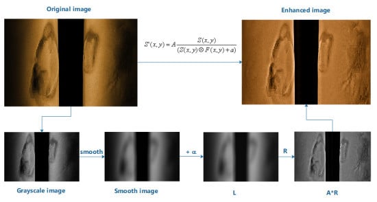
In this section, we provide the overall framework of the proposed algorithm, as shown in Figure 3. First, we obtain the gray image from the original side-scan sonar data, or gray the pseudo-color side-scan sonar image to obtain the gray image of side-scan sonar image. Then, the gray image of the side-scan-sonar image is filtered to obtain the smooth image. The constant coefficient a is added to the smoothed image as the illumination map L in the Retinex model, and then the reflected map R is obtained based on an element-wise division using Equation (4). The reflected map R is multiplied by a constant coefficient A as the enhanced image. Finally, the enhanced gray image is pseudo-color processed to obtain the final gray scale corrected side-scan sonar image.
5.1. Experiments and Analysis of Parameter A
The constant coefficient A can be adjusted using this method. If a brighter gray scale correction image is needed, the value of A can be set higher, and vice versa. We analyzed it through experiments. In the experiment, the size of the original sonar image was 800 × 525 pixels. We set the constant a to 15. Then, we smoothed the image using the mean filter. The size of the filter template was set to 1/17 of the size of original image, and A was set to 80, 140, and 200.
The experimental results are shown in Figure 4. The results show that the side-scan sonar image corrected using this method can correct the original gray distortion image, so that the image scene information scanned by sonar can be displayed normally. The size of A only affects the overall brightness of the enhanced image and does not cause secondary distortion of the enhanced image. The enlarged detail image shown in Figure 5 shows that the gray distortion of the original image is serious. After gray scale correction, the gray distortion of the image disappears, and the texture information of the image is displayed normally. In the experiment, the bigger the value of A, the higher the gray value of the corrected image, and the clearer the image. The adjustment of A does not affect the overall gray distribution of the enhanced image, but only the overall brightness of the enhanced image. However, when the value of A is set too large, the image is too bright, and the enhanced brightness is not suitable for human perception. We did not fix A to a size. If different brightness enhancement images are required, adjust the value of A. If A must have a fixed value, we recommend A = 140, because we do a lot of experiments in Appendix A and Appendix B, A = 140 meets the experimental requirements.
5.2. Experiments and Analysis of Parameter a
In our algorithm, constant a is used to suppress the noise. We experimentally analyzed the selection of the a value. In the experiment, we set the constant A to 140. Then, we smoothed the image using the mean filter. The size of the filter template was set to 1/17 of the size of original image, and a was set to 0, 5, 10, 15, 30, 40, and 60.
As shown in Figure 6, when we changed the value of a while the other parameters remained unchanged, the noise in the dark area of the enhanced image was amplified with the decrease in the value of a, and vice versa. However, since we add a to the smoothed original image as the illumination estimation of the original image, when a increases excessively, the estimated illumination cannot accurately represent the illumination map of the original image. If the a value is too large, the effect of image correction worsens, as supported by our experimental results. The parameters setting of the side-scan sonar may be different in different batches of sonar data, which leads to differences in the image characteristics of side-scan sonars. Thus, the value of a is an empirical value. According to our experiment and as shown in the experimental results in Appendix B, the value of a is about 15. The value of a does not need to be adjusted for the same batch of side-scan sonar images, and different batches may require fine-tuning.
5.3. Experiments and Analysis of Smoothing Function
In this algorithm, the gray image from a side-scan sonar can be smoothed using many methods. Bilateral filtering was used to smooth side-scan sonar images, which was compared with the experimental results of mean filtering. In the contrast experiment, A was set to 140 and a to 15. Figure 7 compares the experimental results produced when using the mean filter and bilateral filter.
As shown in Figure 7, the enhanced images produced by these two methods are similar overall, but in terms of image details, the experimental results show that the illumination map L produced by bilateral filtering is clearer than the illumination map L obtained by mean filtering in the water column area, and the mean filtering is blurred. The smoothed image obtained by bilateral filtering reflects the illumination distribution of the original image better, and the corrected image obtained in the experiment is more stable and clear. To see more clearly, we enlarged part of Figure 7. As shown in Figure 8, because the gray image is smoothed with only the mean filter, the gray image after smoothing has an unclear gray boundary in the region with a large gray gradient. The illumination map smoothed by mean filter cannot accurately express the illumination distribution of the original image, especially around the region with a large gray gradient. Therefore, the corrected image obtained using the mean filter will show some over-enhancement and the halo phenomena in the areas where the gray level of the original image changes too much. The corrected image produced using the bilateral filter is more normal, and there is no halo phenomenon because the map produced with bilateral filtering is more in line with the actual gray distribution of the original image.
5.4. Comparative Experiments and Analysis of Other Methods Based on Retinex
Considering several commonly used image enhancement methods based on Retinex, we used different original side-scan sonar images to verify the stability and advantages of our proposed image enhancement algorithm, and used SSR, MSR, MSRCR, and MSRCP of four commonly used image enhancement methods based on Retinex for comparison with our methods. The parameters of bilateral filter were set as follows: diameter range of each pixel neighborhood was set to 35, sigma-color is set to one-seventh of the height of the original image, and sigma-color represented the sigma value of the color space filter. The larger the value of this parameter, the wider the colors in the neighborhood of the pixel are mixed together. Sigma-space was set to one-seventh of the width of the original image and sigma-spaces represent the sigma values of filters in coordinate space. The larger the sigma values, the more distant the pixels interact with each other. Our other experimental parameters were as follows: A was set to 140 and a was set to 15. The results are shown in Figure 9. For better illustration and display, we enlarged a local area of Figure 9, as shown in Figure 10.
The experimental results show that SSR, MSR, MSRCR, and MSRCP produce considerable noise and the image sharpness of the enhancement is very poor and the image corrected by the SSR method cause blurred and excessive corrections. Therefore, these four methods are not suitable for gray correction of side-scan sonar images. The enhanced image color produced using the MSRCR algorithm is more consistent with the original side-scan sonar image color than using the MSR algorithm. The enhancement effect of our method is better than that of the other four methods. The enlarged detail map shows that the detail map of our method is more clear and stable.
To fairly evaluate the image enhancement algorithm, we used the peak signal-to-noise ratio (PSNR), information entropy, standard deviation, and average gradient as the evaluation indexes. PSNR represents the ability of an image enhancement algorithm to suppress noise. The larger the value, the better the ability to noise suppression and the smaller the image distortion. PNSR can be calculated with Equations (10) and (11).
where MSE represents the mean square error of the current image X and the reference image Y; H and W are the height and width of the image, respectively; n is the number of bits per pixel, which is generally 8, meaning the gray scale of the pixel is 256; and the unit of PSNR is dB.
Information entropy is a measure of image information richness and is calculated as
where L is the maximum gray level of image X, and is the number of pixels whose gray value of image X is K.
The standard deviation reflects the dispersion of all image pixel values to the mean value; the smaller its value, the more balanced the gray distribution of the image. We can calculate standard deviation using Equation (13), where is the gray value of the pixels in the image, is the average gray level of the image, and n is the number of pixel points in the image:
The average gradient represents the ability to express the details of the image, the image sharpness, and texture changes. The bigger the average gradient, the sharper the edge of the image, and the clearer the image. Average gradient can be calculated with
where is the gradient in the horizontal direction, is the gradient in the vertical direction, and M and N are the height and width of the image, respectively.
According to the experimental results provided in Table 1, the proposed algorithm is superior to the other four algorithms in PNSR, information entropy, image standard deviation, and average gradient. So, we proved that the enhanced image produced using our algorithm is clearer, the ability to suppress noise is stronger, the gray distribution is more balanced, the image information is richer, and the details of the image are enhanced. Therefore, the image enhancement algorithm in this paper is better than the other three algorithms.
We compared the latest image enhancement algorithms based on Retinex theory. The experimental parameters of the algorithms were obtained from the parameters set by the respective authors. We did not change the parameters of the algorithm. We used the smoothing filter and bilateral filter to implement our method, and the experimental parameters were the same as those used above. The experimental code was realized using MATLAB (MathWorks, Natick, US). All the experiments were conducted on a PC running Windows 10 (Microsoft, Redmond, US) OS with 4 G RAM and a 2.4 GHz CPU. In this paper, three different side-scan sonar images were used for experiments, representing three types of side-scan sonar images: (a) An image with a large area of black due to the occlusion of seabed hills (Figure 11a), (b) an image with no black area and more texture (Figure 11b,c) an image with black areas, textures, and hills (Figure 11c).
Three different types of side-scan sonar images were compared using low-light image enhancement (LIME), naturalness preserved enhancement (NPE), simultaneous reflection and illumination estimation (SRIE), multi-deviation fusion method (MF), and our two methods with mean filtering and bilateral filtering methods. The experimental results are shown in Figure 12. In terms of enhancement effect, LIME, NPE, SRIE, MF, and the two methods in this paper obviously enhance side-scan sonar images, but the image enhanced by NPS method produces a lot of noise in the dark area of the image. As shown in Figure 13, we enlarged the images of different methods for the second side-scan sonar image. The local enlarged image shows that there are some inadequate corrections at the left and right ends of the image enhanced with the LIME, NPE, SRIE, and MF methods, but no such situation was observed using the two methods in this paper.
As shown in Figure 14, the histogram gray value of the enlarged image of the four methods, LIME, NPE, SRIE, and MF, has obvious peaks in the low gray part. However, the two methods in this paper have no obvious peaks in the low gray part of the histogram. LIME, NPE, SRIE, and MF do not effectively enhance the image at both ends and the enhancement effect is not as good as the two methods in this paper.
To better evaluate the performance of the algorithm, we used PSNR, information entropy, standard deviation, average gradient, and algorithm running time to evaluate the image enhancement algorithm as a whole. We calculated the index using the whole enhanced image instead of the local enlarged image. The evaluation index table is shown in Table 2.
Among the PSNR, information entropy, standard deviation and average gradient of the evaluation indexes, our algorithm in this paper is similar to the other four latest algorithms. The information entropy of image enhancement based on bilateral smoothing is the highest, and the information entropy of image enhancement based on mean filtering method is the second. Our algorithm is faster. Our mean filter is the fastest, followed by our bilateral filter, then the MF algorithm, in which our mean filter method is at least twice as fast as the other methods. The speed of our bilateral filtering method is equal to MF, which is faster than LIME, NPE, and SRIE. We can use the mean filter and bilateral filter to smooth the gray image of side-scan sonar image separately and use the two schemes to enhance side-scan sonar images. The evaluation index shows that the enhancement effect of the bilateral filtering method in this paper is slightly better than that of the mean filtering method, but the mean filtering method takes less time than that of the bilateral filtering method. Therefore, the mean filtering enhancement algorithm is more suitable for online processing situations when the image processing speed is more important, and the bilateral filtering method is more suitable for side-scan sonar image enhancement that requires better image enhancement during offline processing. The side-scan sonar image enhancement algorithm in this paper is simple but not inferior to other high-quality algorithms. The reasons for this situation are as follows: (1) The original side-scan sonar image is a gray-scale image, and there are no R, G, and B channels. The color side-scan sonar image is pretreated by pseudo-color application, so we do not need to use max-RGB technology to obtain the illumination map of the original side-scan sonar image. (2) The key to using the Retinex image enhancement algorithm is to obtain an accurate illumination map. The illumination map needs to smooth the details of the original image as much as possible while maintaining the boundaries of the gray distribution of the original image. So, the other four methods use more complex algorithms to obtain an accurate illumination map, which results in an increase in the running time. However, side-scan sonar images are different from natural illumination images. The gray gradient of the side-scan sonar image changes little, and there is no case of too large a gray gradient. Therefore, it is not necessary to use a complex algorithm to obtain a fine illumination image to ensure that the enhanced image does not display a halo phenomenon. To suppress halo generation, we can achieve the desired effect by increasing the value of A. (3) The illumination map produced by the other four methods is not smooth enough, which leads to poor gray level correction and enhancement effect on the left and right ends of the side-scan sonar waterfall image.
5.5. Comparative Experiments and Analysis of Gray Scale Correction Methods for Side-Scan Sonar Images
The existing gray level correction methods for side-scan sonar images are realized by experiments. As the TVG method and sonar propagation attenuation model needs to know some side-scan sonar parameters, we only compared the histogram method, the non-linear gray level compensation method, and the function fitting method with our mean filtering method. Figure 15 shows that various methods improve the gray distortion of the original side-scan sonar image after gray correction. The corrected images obtained by the histogram and non-linear compensation methods show that some areas of the image are too strong, then the left and right ends of the image are too weak, which leads to an unsatisfactory enhancement effect of the whole corrected image. The function fitting method and the method proposed in this paper are better than the other two methods.
Figure 16 depicts a histogram comparison of the enhanced images. The histogram correction method results in overweight correction, which produces a particularly high gray value in some areas of the image. The non-linear compensation and function fitting methods have too many parts with low gray values, which proves that the image correction is inadequate. The histogram of the side-scan sonar image enhancement method proposed in this paper shows that the gray value distribution of the side-scan sonar image after correction is uniform, and the correction result of the algorithm is satisfactory.
To better analyze the contrast effect of the different enhancement methods, we enlarged the enhanced image locally. The enlarged image is shown in Figure 17. We found that the texture of the side-scan sonar image is destroyed by the function fitting method. The enhanced side-scan sonar images obtained by function fitting, histogram, and non-linear compensation methods have low gray values at the left and right ends of the image, and the effect of gray correction is not obvious. However, our method still enhances the local enlargement image very clearly.
Only visually observing the corrected image may not be sufficient to differentiate the methods. We also contrasted the image enhancement indexes for the local enlarged image, as shown in Table 3. The enhanced image in this paper is superior to other methods in information entropy and average gradient.
Our method was compared with the commonly used gray level correction method for side-scan sonar images. According to the experimental results, our method is superior to the other methods. Compared with other common methods and the latest optical image methods based on Retinex, the gray scale correction effect of side-scan sonar images using our method is better than those of these methods, as shown by the experimental results and data indicators.
6. Expansion of Our Method
The proposed method is not only suitable for gray level correction of side-scan sonar images, but can also be used to enhance low illumination optical color images. The steps for low illumination color image enhancement are shown in Figure 18. Firstly, we separate the three channels of the color image into R, G, and B channels. Then, we use the above-mentioned method (gray image smoothing filtering), and add a constant a as the illumination image L. Using Equation (15), the three channels are separately removed from the illumination image L and multiplied by constant coefficient A to obtain the enhanced images of the three channels. Finally, the three channels are merged into the final color enhanced image.
To verify the speed of our proposed algorithm for low illumination color image enhancement, we conducted an experiment. The smoothing method used in the experiment was mean filtering. The size of the filter template was one-seventh of the original image. A was set to 160 and a was set to 17. All the experiments were conducted on a PC running Windows 10 (Microsoft, Redmond, US) OS with 8 G RAM and a 3.7 GHz CPU. Our code was implemented using C++ and OpenCV, which is an image processing library.
As shown in Figure 19, we selected four low illumination color images of different sizes for enhancement. Table 4 shows the time required for low illumination color image enhancement with different-sized images. Because of its speed, this algorithm can meet the real-time video processing requirements. If GPU is used to accelerate the processing, the algorithm will be faster.
As shown in Figure 19, the first three low-illumination color images are better enhanced by our image enhancement method, but the fourth image is enhanced with an obvious halo phenomenon. The halo phenomenon occurs after the image is enhanced in areas where the gray gradient changes greatly. This mainly occurs because the smoothing method adopted in this paper is too simple, which results in the obtained illumination map being too rough and the illumination distribution of the original image is not well expressed. Thus, our enhancement method is more suitable for side-scan sonar images that where the gray gradients changes are not so abrupt.
7. Conclusions
Side-scan sonars are widely used in ocean exploration. As the original side-scan sonar images are affected by gray distortion, gray scale correction is needed before any further image processing. Considering the difference between side-scan sonar images and visible images, we proposed a gray correction method for side-scan sonar images based on Retinex, which is simple and easy to implement. Compared with the commonly used gray scale correction methods for side-scan sonar images, this method avoids the limitations of the current gray scale correction methods, such as the need to know the side-scan sonar parameters, the need to recalculate or reset the parameters for different side-scan sonar image processing, and the poor image enhancement effect. Compared with the latest image enhancement algorithms based on Retinex, our proposed methods have similar image enhancement indexes, and our method is the fastest. When it is necessary to adjust the brightness of the corrected image, only the magnitude of constant coefficient A in the algorithm needs to be adjusted. Our method can also be used to enhance low illumination color images, and the experimental results show that the algorithm is fast.
Author Contributions
Conceptualization, X.Y. and H.Y.; Data curation, H.Y.; Formal analysis, H.Y.; Funding acquisition, X.Y.; Investigation, X.Y. and C.L.; Methodology, X.Y.; Project administration, P.L.; Resources, C.L. and Y.J.; Software, H.Y., Y.J. and P.L.; Supervision, C.L.; Validation, H.Y.; Visualization, Y.J.; Writing – original draft, X.Y.; Writing – review & editing, X.Y.
Funding
This work was supported by the National Natural Science Foundation of China (Grant No. 41876100), the National key research and development program of China (Grant No. 2018YFC0310102 and 2017YFC0306002), the State Key Program of National Natural Science Foundation of China (Grant No.61633004), the Development Project of Applied Technology in Harbin (Grant No.2016RAXXJ071) and the Fundamental Research Funds for the Central Universities (Grant No. HEUCFP201707).
Acknowledgments
To verify the adaptability of the parameters of our algorithm, we used side-scan sonar images from previous studies. Thank you to the authors of these papers.
Conflicts of Interest
The authors declare no conflict of interest.
Appendix A
To verify the generality of our method, we used our method (bilateral filtering) to enhance several original side-scan sonar images and fixed A to 140 and a to 15. The results are shown in the following.

Appendix B
To verify that our method is also suitable for correction of side-scan sonar images in other batches, we used our algorithm (bilateral filtering) to enhance them. Because we lacked other batches of side-scan sonar images, we were only able to obtain images by clipping them from previous studies [7,8,9] and the quality of the side-scan sonar images was poor. However, the effects of the enhanced images verified the adaptivity of our algorithm.
Figure A1.
Side-scan sonar image enhancement from Zhao, J et al. [9]: (a) original image with changes in sediments and (b) enhanced image (bilateral filtering, A = 140, a = 17).
Figure A1.
Side-scan sonar image enhancement from Zhao, J et al. [9]: (a) original image with changes in sediments and (b) enhanced image (bilateral filtering, A = 140, a = 17).


References
- Dura, E.; Zhang, Y.; Liao, X.; Dobeck, G.J.; Carin, L. Active learning for detection of mine-like objects in side-scan sonar imagery. IEEE J. Ocean. Eng. 2015, 30, 360–371. [Google Scholar] [CrossRef]
- Reggiannini, M.; Salvetti, O. Seafloor analysis and understanding for underwater archeology. J. Cult. Herit. 2017, 24, 147–156. [Google Scholar] [CrossRef]
- Hovland, M.; Gardner, J.V.; Judd, A.G. The significance of pockmarks to understanding fluid flow processes and geohazards. Geofluids 2002, 2, 127–136. [Google Scholar] [CrossRef] [Green Version]
- Kaeser, A.J.; Litts, T.L.; Tracy, T.W. Using low-cost side-scan sonar for benthic mapping throughout the lower flint river. River. Res. Appl. 2013, 29, 634–644. [Google Scholar] [CrossRef]
- Blondel, P. The Handbook of Sidescan Sonar; Springer: Berlin/Heidelberg, Germany, 2009; pp. 62–66. ISBN 978-3-540-42641-7. [Google Scholar]
- Chang, Y.C.; Hsu, S.K.; Tsai, C.H. Sidescan sonar image processing: Correcting Brightness Variation and Patching Gaps. J. Mar. Sci Tech.-Taiw. 2010, 18, 785–789. [Google Scholar]
- Capus, C.G.; Banks, A.C.; Coiras, E.; Ruiz, I.T.; Smith, C.J.; Petillot, Y.R. Data correction for visualisation and classification of sidescan SONAR imagery. IET Radar Sonar Navig. 2008, 2, 155–169. [Google Scholar] [CrossRef]
- Capus, C.; Ruiz, I.T.; Petillot, Y. Compensation for Changing Beam Pattern and Residual TVG Effects with Sonar Altitude Variation for Sidescan Mosaicing and Classification. In Proceedings of the 7th European Conference Underwater Acoustics, Delft, The Netherlands, 5–8 July 2004. [Google Scholar]
- Zhao, J.; Yan, J.; Zhang, H.M.; Meng, J.X. A new radiometric correction method for side-scan sonar images in consideration of seabed sediment variation. Remote Sens. 2017, 9, 575. [Google Scholar] [CrossRef]
- Ye, X.F.; Li, P.; Zhang, J.G.; Shi, J.; Gou, S.X. A feature-matching method for side-scan sonar images based on nonlinear scale space. J. Mar. Sci. Technol. 2016, 21, 38–47. [Google Scholar] [CrossRef]
- Wang, A.; Zhang, H.; Wang, X. Processing principles of side-scan sonar data for seamless mosaic image. J. Geomat. 2017, 42, 26–33. [Google Scholar]
- Zhao, J.; Shang, X.; Zhang, H. Reconstructing seabed topography from side-scan sonar images with self-constraint. Remote Sens. 2018, 10, 201. [Google Scholar] [CrossRef]
- Johnson, H.P.; Helferty, M. The geological interpretation of side-scan sonar. Rev. Geophys. 1990, 28. [Google Scholar] [CrossRef]
- Shippey, G.; Bolinder, A.; Finndin, R. Shade correction of side-scan sonar imagery by histogram transformation. In Proceedings of the Oceans, Brest, France, 13–16 September 1994; IEEE: New York, NY, USA; pp. 439–443. [Google Scholar]
- Li, P. Research on Image Matching Method of the Side-Scan Sonar Image. Doctoral Dissertation, Harbin Engineering University, Harbin, China, 2016. [Google Scholar]
- Al-Rawi, M.S.; Galdran, A.; Yuan, X. Intensity Normalization of Sidescan Sonar Imagery. In Proceedings of the Sixth International Conference on Image Processing Theory, Tools and Applications (IPTA), Oulu, Finland, 12–15 December 2016; pp. 12–15. [Google Scholar]
- Al-Rawi, M.S.; Galdran, A.; Isasi, A. Cubic Spline Regression Based Enhancement of Side-Scan Sonar Imagery. In Proceedings of the Oceans IEEE, Aberdeen, UK, 19–22 June 2017; pp. 19–22. [Google Scholar]
- Burguera, A.; Oliver, G. Intensity Correction of Side-Scan Sonar Images. In Proceedings of the IEEE Emerging Technology & Factory Automation, Barcelona, Spain, 16–19 September 2014; pp. 16–19. [Google Scholar]
- Kleeman, L.; Kuc, R. Springer Handbook of Robotics; Springer: Berlin/Heidelberg, Germany, 2008; pp. 491–519. ISBN 978-3-319-32552-1. [Google Scholar]
- Land, E.H. The retinex theory of color vision. Sci. Am. 1997, 237, 108–128. [Google Scholar] [CrossRef]
- Jobson, D.J.; Rahman, Z.; Woodell, G.A. A multiscale retinex for bridging the gap between color images and the human observation of scenes. IEEE Trans. Image Process. 1997, 6, 965–976. [Google Scholar] [CrossRef] [PubMed]
- Barnard, K.; Funt, B. Analysis and Improvement of Multi-Scale Retinex. In Proceedings of the 5th Color and Imaging Conference Final Program and Proceedings, Scottsdale, AZ, USA, 1–5 January 1997; pp. 221–226. [Google Scholar]
- Jobson, D.J.; Woodell G, G.A. Retinex processing for automatic image enhancement. Electron. Imaging. 2004, 13, 100–110. [Google Scholar] [CrossRef]
- Jin, L.; Miao, Z. Research on the Illumination Robust of Target Recognition. In Proceedings of the IEEE International Conference on Signal Processing, Chengdu, China, 6–10 December 2016; pp. 811–814. [Google Scholar]
- Guo, X.; Li, Y.; Ling, H. LIME: Low-light image enhancement via illumination map estimation. IEEE Trans. Image Process. 2017, 26, 982–993. [Google Scholar] [CrossRef] [PubMed]
- Wang, S.; Zheng, J.; Hu, H.M. Naturalness preserved enhancement algorithm for non-uniform illumination images. IEEE Trans. Image Process. 2013, 22, 3538–3548. [Google Scholar] [CrossRef] [PubMed]
- Fu, X.; Zeng, D.; Huang, Y.; Zhang, X.; Ding, X. A Weighted Variational Model for Simultaneous Reflectance and Illumination Estimation. In Proceedings of the IEEE Conference on Computer Vision and Pattern Recognition (CVPR), Las Vegas, NV, USA, 27–30 June 2016; pp. 2782–2790. [Google Scholar]
- Fu, X.; Zeng, D.; Huang, Y.; Liao, Y.; Ding, X.; Paisley, J. A fusion-based enhancing method for weakly illuminated images. Signal Process. 2016, 129, 82–96. [Google Scholar] [CrossRef]
Figure 1.
Working schematic diagram of a side-scan sonar.

Figure 2.
Original side-scan sonar image.

Figure 3.
The overall framework of the algorithm in this paper.

Figure 4.
Experimental comparison using mean filter. (a) Original image and corrected image with (b) A = 80, (c) A = 140, and (d) A = 200.
Figure 4.
Experimental comparison using mean filter. (a) Original image and corrected image with (b) A = 80, (c) A = 140, and (d) A = 200.

Figure 5.
Local enlargement of Figure 4. (a) Original image and corrected image with (b) A = 80, (c) A = 140, and (d) A = 200.
Figure 5.
Local enlargement of Figure 4. (a) Original image and corrected image with (b) A = 80, (c) A = 140, and (d) A = 200.

Figure 6.
Experimental comparison using mean filter. (a) Original image and corrected image with and (b) a = 0, (c) a = 5, (d) a = 10, (e) a = 15, (f) a = 30, (g) a = 40, and (h) a = 60.
Figure 6.
Experimental comparison using mean filter. (a) Original image and corrected image with and (b) a = 0, (c) a = 5, (d) a = 10, (e) a = 15, (f) a = 30, (g) a = 40, and (h) a = 60.


Figure 7.
Experimental comparison of images. (a) Smoothed image using mean filter, (b) mean method results, (c) smoothed image using bilateral filter, and (d) bilateral method image.
Figure 7.
Experimental comparison of images. (a) Smoothed image using mean filter, (b) mean method results, (c) smoothed image using bilateral filter, and (d) bilateral method image.

Figure 8.
Comparison of experimental details: (a) smoothed image using mean filter, (b) mean method results, (c) smoothed image using bilateral filter, and (d) bilateral method results.
Figure 8.
Comparison of experimental details: (a) smoothed image using mean filter, (b) mean method results, (c) smoothed image using bilateral filter, and (d) bilateral method results.

Figure 9.
Comparative experiment of common methods based on Retinex. Images enhanced with (a) SSR, (b) MSR, (c) MSRCR, (d) MSRCP, and (e) using our bilateral filtering method.
Figure 9.
Comparative experiment of common methods based on Retinex. Images enhanced with (a) SSR, (b) MSR, (c) MSRCR, (d) MSRCP, and (e) using our bilateral filtering method.

Figure 10.
Comparison of experimental details. Images enhanced with (a) SSR, (b) MSR, (c) MSRCR, (d) MSRCP, and (e) using our bilateral filtering method.
Figure 10.
Comparison of experimental details. Images enhanced with (a) SSR, (b) MSR, (c) MSRCR, (d) MSRCP, and (e) using our bilateral filtering method.

Figure 11.
Original side-scan sonar images: (a) a large area of black area, (b) an image with no black area and more texture, and (c) image with black areas, textures, and hills.
Figure 11.
Original side-scan sonar images: (a) a large area of black area, (b) an image with no black area and more texture, and (c) image with black areas, textures, and hills.

Figure 12.
Side-scan sonar images enhanced using (a) LIME, (b) NPE, (c) SRIE, (d) MF, and our method with (e) mean filtering, and (f) bilateral filtering.
Figure 12.
Side-scan sonar images enhanced using (a) LIME, (b) NPE, (c) SRIE, (d) MF, and our method with (e) mean filtering, and (f) bilateral filtering.

Figure 13.
Local enlargement of the second kind of enhanced image (a) LIME, (b) NPE, (c) SRIE, (d) MF, and our method with (e) mean filtering, and (f) bilateral filtering.
Figure 13.
Local enlargement of the second kind of enhanced image (a) LIME, (b) NPE, (c) SRIE, (d) MF, and our method with (e) mean filtering, and (f) bilateral filtering.

Figure 14.
The histograms corresponding to Figure 13: (a) LIME, (b) NPE, (c) SRIE, (d) MF, and our method with (e) mean filtering, and (f) is bilateral filtering.
Figure 14.
The histograms corresponding to Figure 13: (a) LIME, (b) NPE, (c) SRIE, (d) MF, and our method with (e) mean filtering, and (f) is bilateral filtering.

Figure 15.
Comparison experiments of common methods used to correct side-scan sonar images: (a) The original side-scan sonar image, (b) histogram, (c) non-linear compensation, (d) function fitting, and (e) our method.
Figure 15.
Comparison experiments of common methods used to correct side-scan sonar images: (a) The original side-scan sonar image, (b) histogram, (c) non-linear compensation, (d) function fitting, and (e) our method.

Figure 16.
Histograms corresponding to the images in Figure 15: (a) the original side-scan sonar image (b) histogram, (c) non-linear compensation, (d) function fitting, and (e) our method.
Figure 16.
Histograms corresponding to the images in Figure 15: (a) the original side-scan sonar image (b) histogram, (c) non-linear compensation, (d) function fitting, and (e) our method.

Figure 17.
Local enlargement of Figure 15: (a) the original side-scan sonar image, and the images produced using the (b) histogram, (c) non-linear compensation, (d) function fitting, and (e) our methods.
Figure 17.
Local enlargement of Figure 15: (a) the original side-scan sonar image, and the images produced using the (b) histogram, (c) non-linear compensation, (d) function fitting, and (e) our methods.

Figure 18.
Low illumination color image enhancement process.

Figure 19.
Enhancement effect of four low illumination color scene images: (a) scene 1, (b) scene 2, (c) scene 3, and (d) scene 4.
Figure 19.
Enhancement effect of four low illumination color scene images: (a) scene 1, (b) scene 2, (c) scene 3, and (d) scene 4.


Table 1.
Objective Evaluation Index of Image Enhancement Algorithms.
| Method | PSNR | Information Entropy | Standard Deviation | Average Gradient |
|---|---|---|---|---|
| Original image | 6.81746 | 42.1187 | 5.89745 | |
| SSR | 7.50039 | 6.80343 | 74.8485 | 6.4373 |
| MSR | 8.42826 | 5.8048 | 54.2663 | 9.2899 |
| MSRCR | 6.48304 | 6.54661 | 54.3578 | 6.29672 |
| MSRCP | 7.22485 | 5.66164 | 43.4622 | 5.42281 |
| Ours | 14.5954 | 7.58250 | 43.8442 | 9.48556 |
Table 2.
Objective evaluation index of image enhancement algorithms.
| Original Image | Algorithm | PNSR | Information Entropy | Standard Deviation | Average Gradient | Algorithm Time-Consuming(s) |
|---|---|---|---|---|---|---|
| Image1 | LIME | 12.8283 | 7.59424 | 54.9971 | 11.3484 | 2.15712 |
| NPE | 16.9553 | 7.21194 | 45.2014 | 8.33524 | 20.9530 | |
| SRIE | 19.1414 | 7.28538 | 46.8345 | 7.37814 | 35.7950 | |
| MF | 19.3875 | 7.23853 | 46.1300 | 8.39727 | 3.0470 | |
| our method of mean filter | 14.8291 | 7.50084 | 45.5599 | 9.76665 | 0.5430 | |
| our method of bilateral filter | 15.0356 | 7.50243 | 44.6718 | 9.06058 | 1.7860 | |
| Image2 | LIME | 12.5039 | 7.55372 | 53.4062 | 11.6171 | 2.0779 |
| NPE | 17.4068 | 7.17702 | 14.9912 | 8.01561 | 20.6560 | |
| SRIE | 18.9174 | 7.26646 | 43.9448 | 7.51642 | 33.6090 | |
| MF | 18.6418 | 7.25066 | 42.7528 | 8.66020 | 1.5150 | |
| our method of mean filter | 14.3681 | 7.56064 | 44.7653 | 10.3218 | 0.5440 | |
| our method of bilateral filter | 14.5954 | 7.58250 | 43.8442 | 9.48556 | 1.6880 | |
| Image3 | LIME | 12.9156 | 7.52301 | 56.4356 | 11.98260 | 2.40157 |
| NPE | 18.0214 | 7.36287 | 45.1654 | 8.42337 | 20.5220 | |
| SRIE | 19.3221 | 7.37251 | 47.1540 | 7.91938 | 35.2410 | |
| MF | 19.0227 | 7.33752 | 46.9760 | 8.49770 | 1.4690 | |
| our method of mean filter | 14.9149 | 7.57515 | 46.7814 | 10.30420 | 0.6860 | |
| our method of bilateral filter | 15.1388 | 7.61042 | 45.8554 | 9.41506 | 1.5670 |
Table 3.
Indicators comparison of local magnification maps.
| Method | PSNR | Information Entropy | Standard Deviation | Average Gradient |
|---|---|---|---|---|
| Original image | 6.1333 | 11.0744 | 2.55545 | |
| HE | 9.82301 | 7.26025 | 45.695 | 9.87564 |
| Non-linear compensation | 11.4153 | 7.17749 | 45.9537 | 8.71157 |
| Function fitting | 9.91988 | 6.67453 | 48.7124 | 8.34709 |
| Our method | 8.41441 | 7.41057 | 38.7549 | 13.6594 |
Table 4.
Time required to enhance different-sized low illumination color images.
| Scene | Image Size | Image Occupied Storage | Time-Consuming (s) |
|---|---|---|---|
| 1 | 370 × 415 | 450 KB | 0.035 |
| 2 | 560 × 420 | 689 KB | 0.061 |
| 3 | 720 × 610 | 1.4 MB | 0.104 |
| 4 | 1024 × 683 | 963 KB | 0.206 |
© 2019 by the authors. Licensee MDPI, Basel, Switzerland. This article is an open access article distributed under the terms and conditions of the Creative Commons Attribution (CC BY) license (http://creativecommons.org/licenses/by/4.0/).
Share and Cite
MDPI and ACS Style
Ye, X.; Yang, H.; Li, C.; Jia, Y.; Li, P. A Gray Scale Correction Method for Side-Scan Sonar Images Based on Retinex. Remote Sens. 2019, 11, 1281. https://doi.org/10.3390/rs11111281
AMA Style
Ye X, Yang H, Li C, Jia Y, Li P. A Gray Scale Correction Method for Side-Scan Sonar Images Based on Retinex. Remote Sensing. 2019; 11(11):1281. https://doi.org/10.3390/rs11111281
Chicago/Turabian StyleYe, Xiufen, Haibo Yang, Chuanlong Li, Yunpeng Jia, and Peng Li. 2019. "A Gray Scale Correction Method for Side-Scan Sonar Images Based on Retinex" Remote Sensing 11, no. 11: 1281. https://doi.org/10.3390/rs11111281
Note that from the first issue of 2016, this journal uses article numbers instead of page numbers. See further details here.