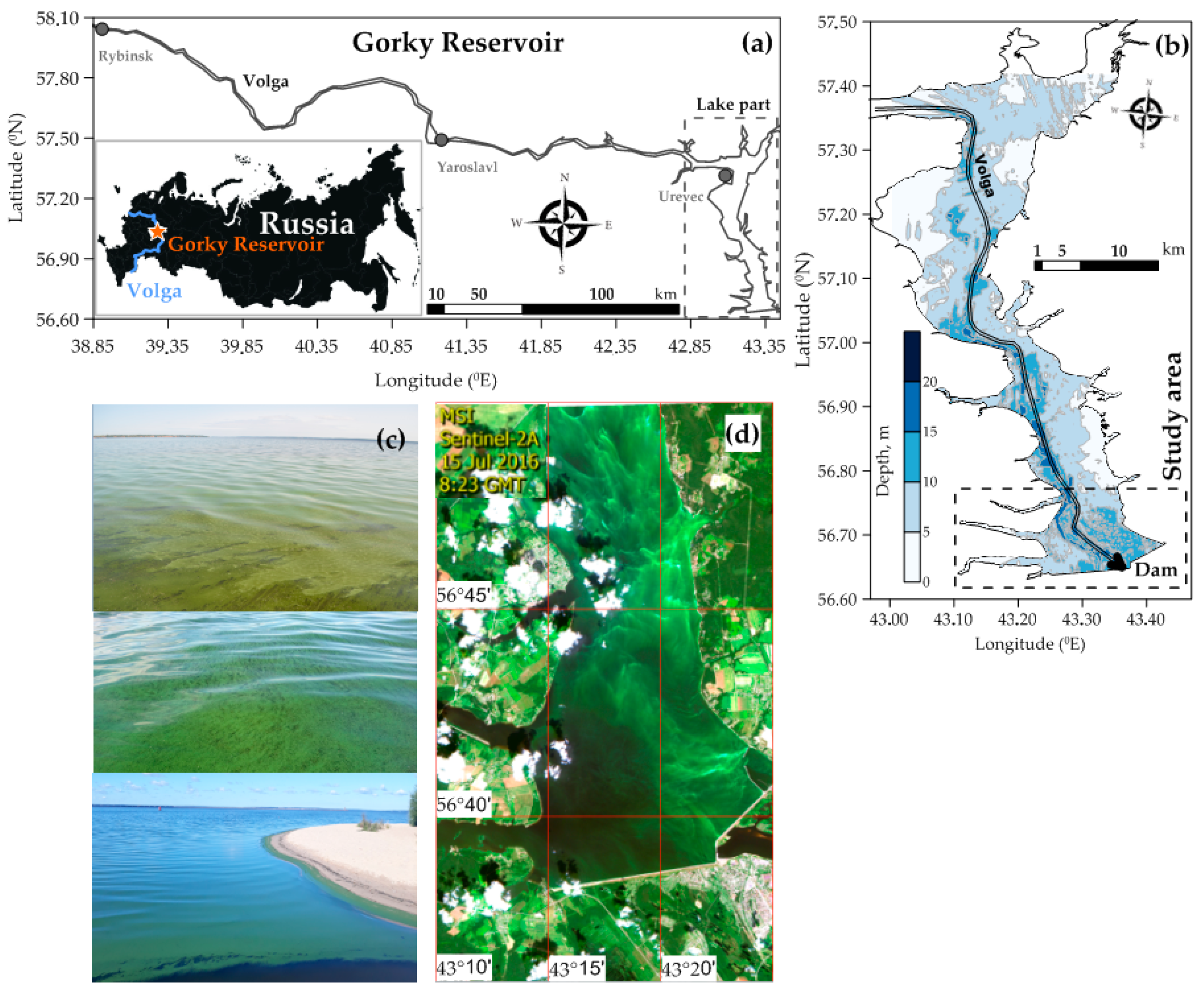
Figure 1.
The Gorky Reservoir: (a) basic map; (b) the lake part map; (c) photo of a cyanobacteria bloom; and (d) Sentinel-2A true color image (15 July 2016) of cyanobacteria bloom.
Figure 1.
The Gorky Reservoir: (a) basic map; (b) the lake part map; (c) photo of a cyanobacteria bloom; and (d) Sentinel-2A true color image (15 July 2016) of cyanobacteria bloom.
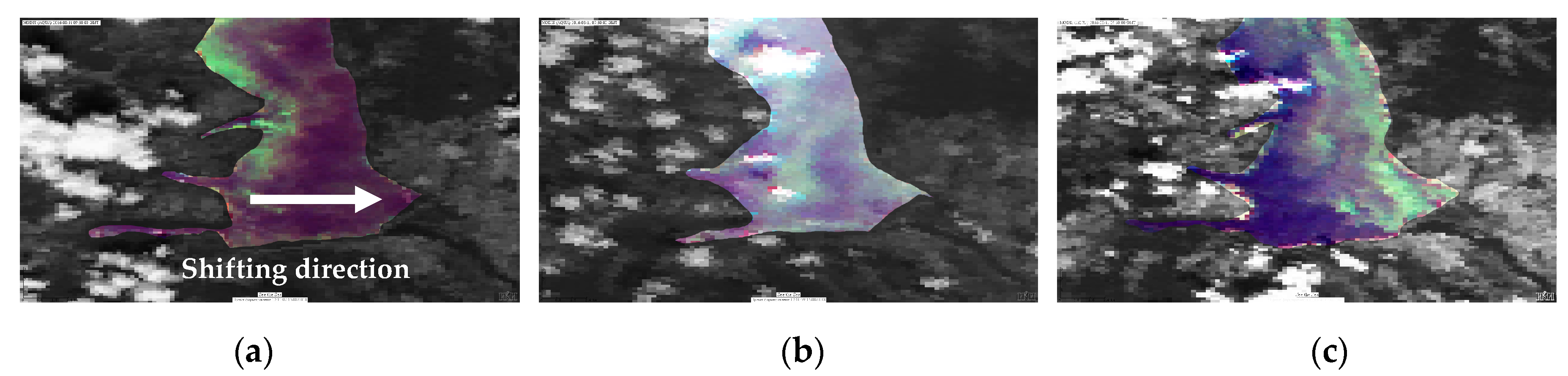
Figure 2.
MODIS images of the Gorky Reservoir illustrating the process of algal bloom shifting from the right riverside to the left one under wind forcing: (a) 29 July 2016, (b) 30 July 2016, and (c) 1 August 2016.
Figure 2.
MODIS images of the Gorky Reservoir illustrating the process of algal bloom shifting from the right riverside to the left one under wind forcing: (a) 29 July 2016, (b) 30 July 2016, and (c) 1 August 2016.
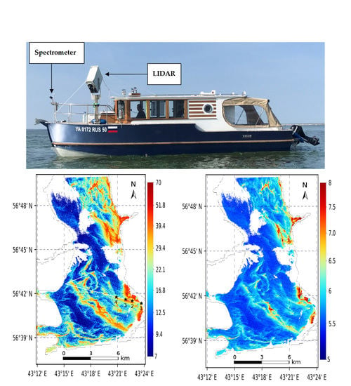
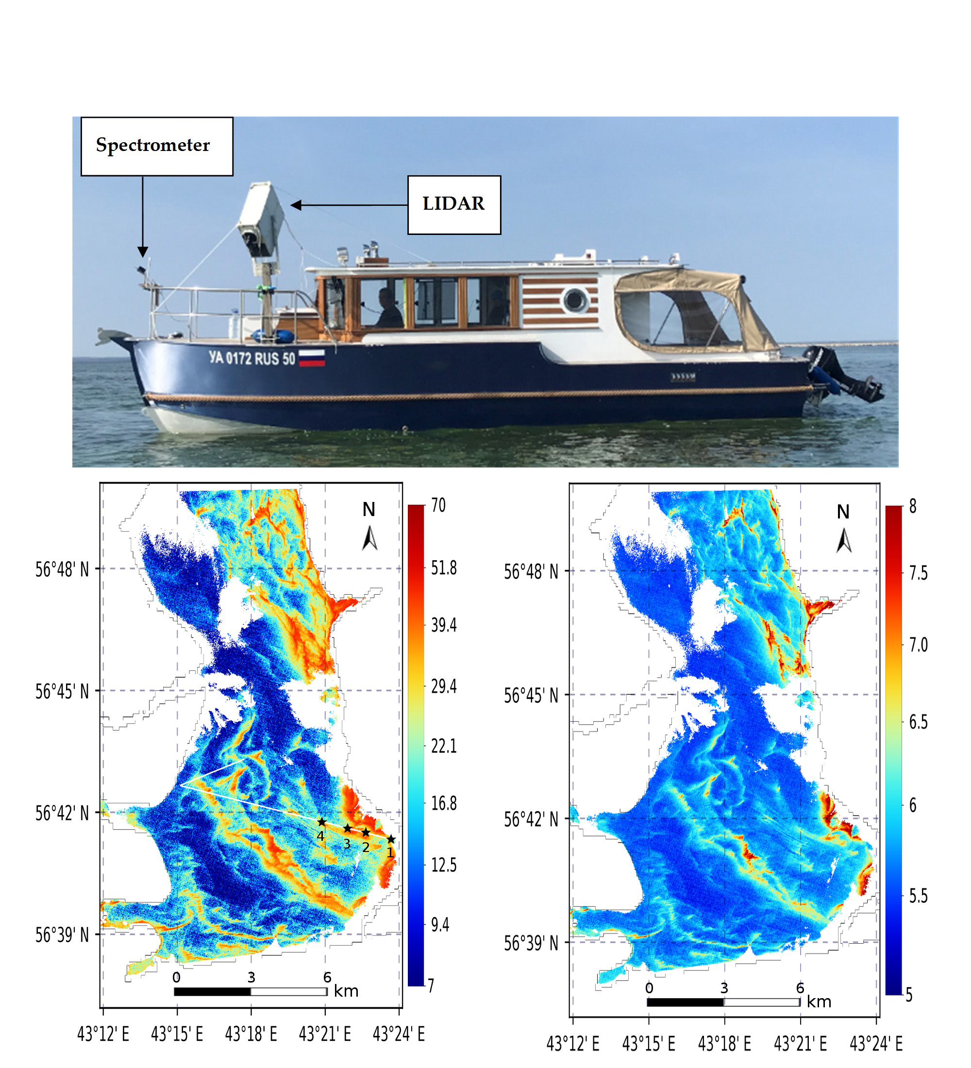
Figure 3.
The spectrometer and LiDAR position on a board of the high-speed gliding motorboat.
Figure 3.
The spectrometer and LiDAR position on a board of the high-speed gliding motorboat.
Figure 4.
Motorboat route map for 21–22 September 2018.
Figure 4.
Motorboat route map for 21–22 September 2018.
Figure 5.
Results of comparison of LiDAR signals at stations with lab-analyzed water sample concentrations of (a) Chl a, and (b) TSM. Black lines correspond to the best calibration fits (1), and (2), respectively.
Figure 5.
Results of comparison of LiDAR signals at stations with lab-analyzed water sample concentrations of (a) Chl a, and (b) TSM. Black lines correspond to the best calibration fits (1), and (2), respectively.
Figure 6.
Schematic explanation of radiometric measurements: (a) the total upwelling radiance, (b) the surface-reflected radiance, and (c) the plaque radiance. Section (d) presents a photo of a water-filled cuvette at field measurements of the surface-reflected radiance.
Figure 6.
Schematic explanation of radiometric measurements: (a) the total upwelling radiance, (b) the surface-reflected radiance, and (c) the plaque radiance. Section (d) presents a photo of a water-filled cuvette at field measurements of the surface-reflected radiance.
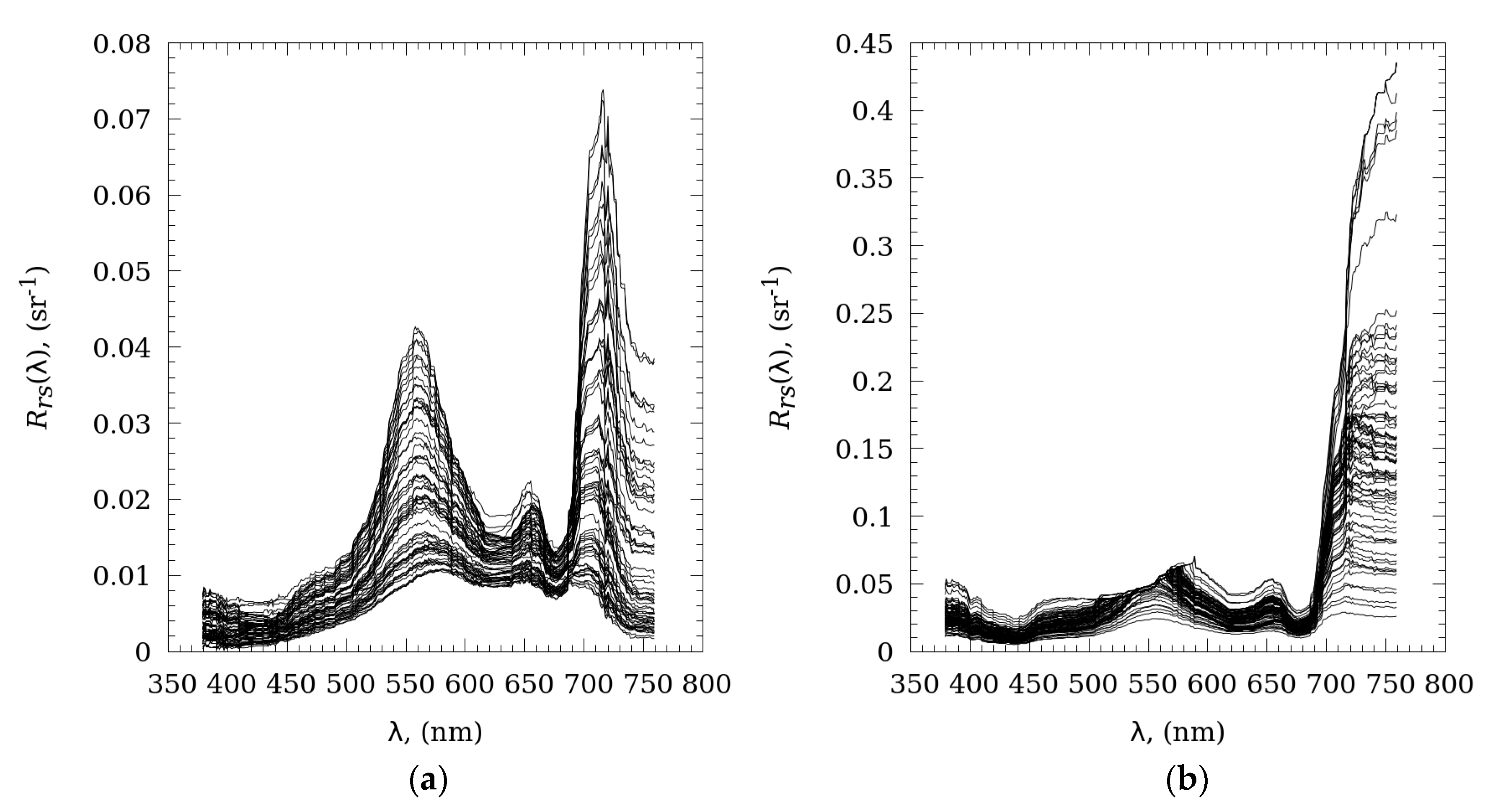
Figure 7.
Examples of Rrs spectra measured in the Gorky reservoir for two days: (a) spectra included in the temporal-synchronous dataset for calibration/validation of empirical models; and (b) spectra excluded from calibration/validation dataset.
Figure 7.
Examples of Rrs spectra measured in the Gorky reservoir for two days: (a) spectra included in the temporal-synchronous dataset for calibration/validation of empirical models; and (b) spectra excluded from calibration/validation dataset.
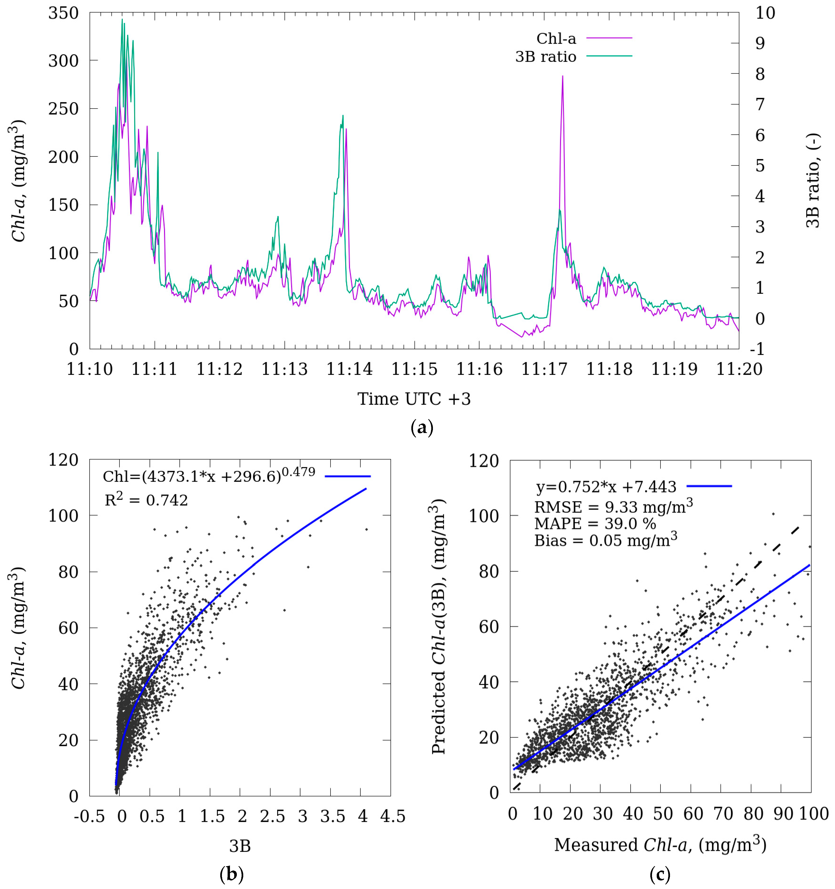
Figure 8.
(a) Fragment (N = 520) of time-series of Chl a and 3B ratio calculated by radiometric measurements of 22 September 2018. Three-band model (3B) for estimation of Chl a concentration using bands 4,5,6 of MSI/Sentinel-2: (b) the results of calibration (N = 2452); and (c) the results of validation (N = 1635) of the 3B model. The dashed line on (c) represents the 1:1 line.
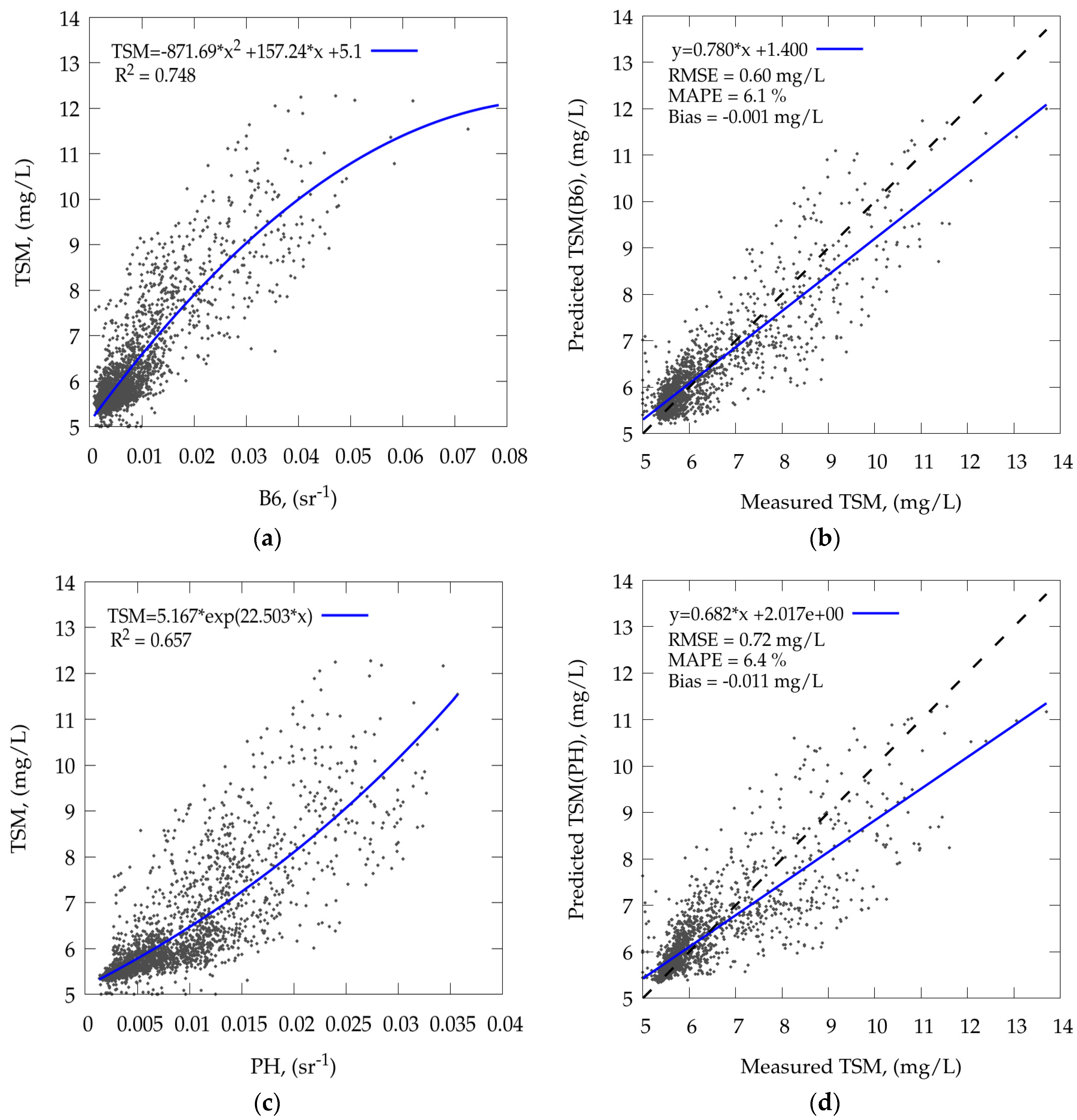
Figure 9.
One-band model for TSM estimation using B6 band of MSI/Sentinel-2: (a) results of calibration (N = 2452) and (b) results of validation (N = 1635); band-ratio model for estimation of TSM concentration using a height of the reflectance peak near 710 nm (PH) calculated by B4, B5, B6 bands of MSI/Sentinel-2: (c) results of calibration (N = 2452) and (d) results of validation (N = 1635). Dashed line represents 1:1 line.
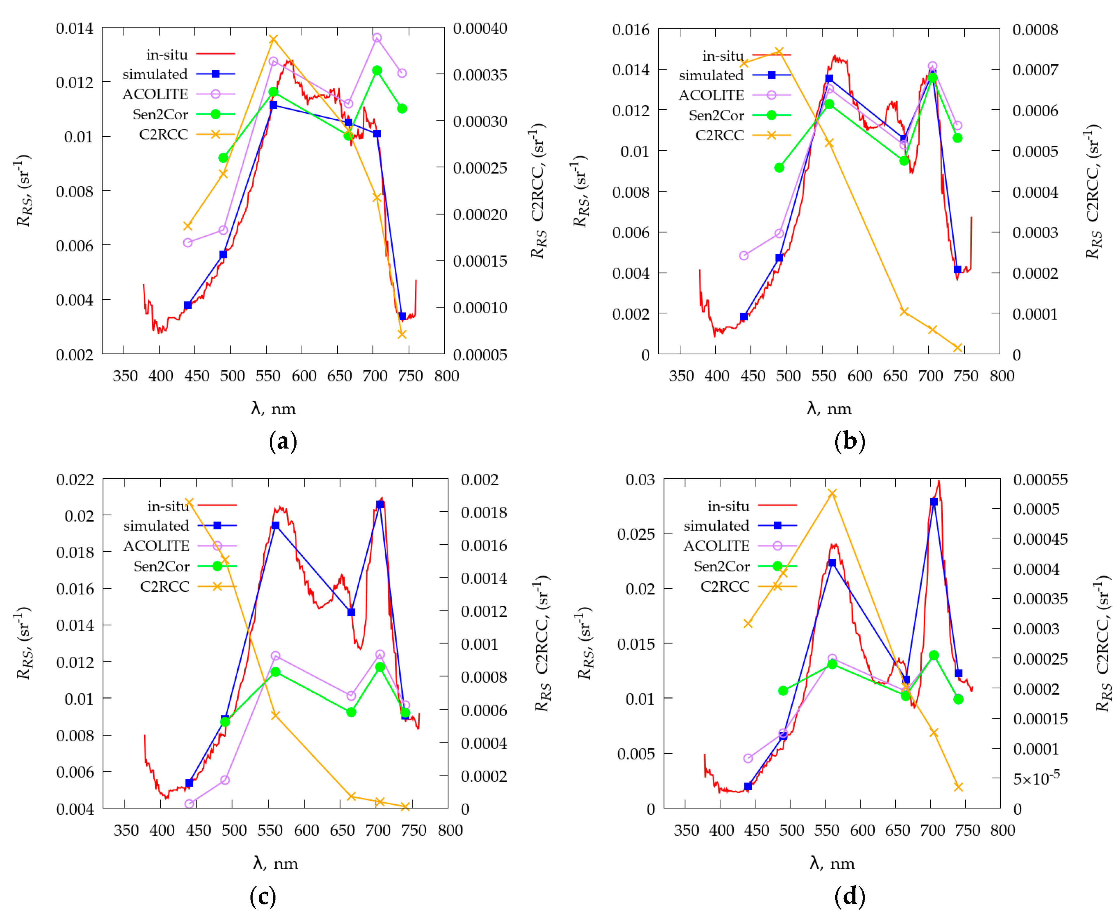
Figure 10.
Comparison of Sentinel-2-retrieved
Rrs by means of atmospheric correction processors (ACOLITE, C2RCC, Sen2Cor) with in situ measurements in pixels depicted as stars in Figure 13a: (
a) pixel #1, (
b) pixel #2, (
c) pixel #3, and (
d) pixel #4. Red lines are hyperspectral measurement of
Rrs, blue lines are measured
Rrs simulated on spectral bands of Sentinel-2/MSI according [
14].
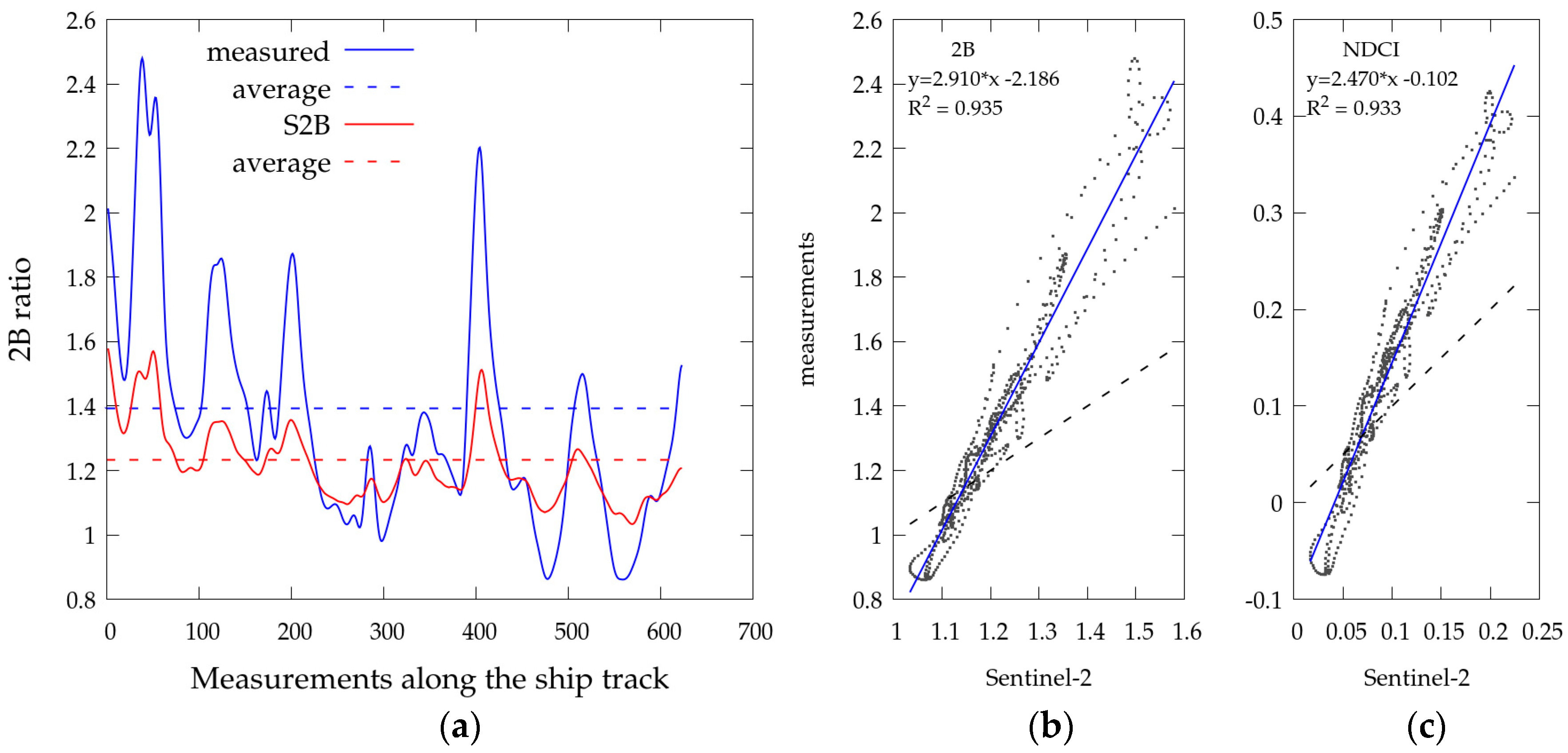
Figure 11.
Comparison of retrieved band-ratio reflectance with in situ measurements (N = 671): (a) time series of the two-band ratio (2B) along ship track, (b) comparison of satellite-retrieved 2B index with measurements, and (c) comparison of the satellite-retrieved NDCI with measurements. Dashed lines on (b) and (c) represent the 1:1 line.
Figure 12.
Results of (a) calibration (N = 401) and (b) validation (N = 270) of the remote sensing algorithm on the basis of the Normalized Difference Chlorophyll Index (NDCI) for Chl a retrieval in the Gorky Reservoir. The dashed line represents the 1:1 line.
Figure 12.
Results of (a) calibration (N = 401) and (b) validation (N = 270) of the remote sensing algorithm on the basis of the Normalized Difference Chlorophyll Index (NDCI) for Chl a retrieval in the Gorky Reservoir. The dashed line represents the 1:1 line.
Figure 13.
Results of (a) calibration (N = 401) and (b) validation (270) of the remote sensing two-band (2B) algorithm for TSM retrieval in the Gorky Reservoir. The dashed line represents the 1:1 line.
Figure 13.
Results of (a) calibration (N = 401) and (b) validation (270) of the remote sensing two-band (2B) algorithm for TSM retrieval in the Gorky Reservoir. The dashed line represents the 1:1 line.
Figure 14.
Spatial distribution of (
a) Chl
a, mg/m
3, and (
b) TSM, mg/L, in the Gorky Reservoir on 21 September 2018. The white line shows to the section along which measurements were chosen for the match-up dataset, the stars show pixels correspond to four spectra in
Figure 10.
Figure 14.
Spatial distribution of (
a) Chl
a, mg/m
3, and (
b) TSM, mg/L, in the Gorky Reservoir on 21 September 2018. The white line shows to the section along which measurements were chosen for the match-up dataset, the stars show pixels correspond to four spectra in
Figure 10.
Table 1.
Hydrological and bio-optical characteristics of the lake part of the Gorky Reservoir according to authors own measurements of 2016–2018 years [
34,
35] and previous studies [
30,
31,
32,
33].
Table 1.
Hydrological and bio-optical characteristics of the lake part of the Gorky Reservoir according to authors own measurements of 2016–2018 years [
34,
35] and previous studies [
30,
31,
32,
33].
| Parameter | Value |
|---|
| Maximum depth, m | 26.6 |
| Average depth, m | 3.65 |
| Maximum current velocity, cm/s | 12.0 |
| Average current velocity, cm/s | 3.0 |
| Average wind speed, m/s | 1.7 |
| Average wind gust speed, cm/s (for a 10 min interval) | 3.3 |
| Average wind gust speed, cm/s (for a 1-min interval) | 14.3 |
| Prevailing wind direction | SW |
| Maximum water temperature, °C | 32 |
| Chlorophyll a concentration, mg/m3 | 0.5–460 |
| TOC concentration, mg/L | 9–21 |
| TSM concentration, mg/L | 5–20 |
| Secchi depth, m | 0.2–3.5 |
| Photic zone depth, m | 1.0–4.1 |
| Trophic state index | eutrophic |
Table 2.
Statistics of Chl a and TSM concentrations measured on 21 September 2018 and 22 September 2018.
Table 2.
Statistics of Chl a and TSM concentrations measured on 21 September 2018 and 22 September 2018.
| Parameter | N | Min | Max | Mean | Median | STD |
|---|
| 21 September 2018 |
| Chl a (mg/m3) | 15,545 | 0.45 | 96.94 | 15.57 | 13.25 | 10.88 |
| TSM (mg/L) | 15,545 | 5.00 | 26.77 | 5.87 | 5.88 | 1.10 |
| 22 September 2018 |
| Chl a (mg/m3) | 5957 | 4.26 | 463.42 | 57.41 | 38.77 | 52.48 |
| TSM (mg/L) | 5957 | 5.38 | 38.76 | 8.42 | 6.54 | 4.39 |
Table 3.
Statistics of temporal-synchronous dataset used for the development of empirical models.
Table 3.
Statistics of temporal-synchronous dataset used for the development of empirical models.
| Parameter | N | Min | Max | Mean | Median | STD |
|---|
| Chl a (mg/m3) | 4087 | 1.06 | 99.32 | 29.85 | 27.11 | 18.37 |
| TSM (mg/L) | 4087 | 5.00 | 19.48 | 6.55 | 5.88 | 1.65 |
Table 4.
Calibration and validation results of Chl a models. All parameters were derived from the calibration dataset (N = 2452, 60%) and the validation dataset (N = 1635, 40%).
Table 4.
Calibration and validation results of Chl a models. All parameters were derived from the calibration dataset (N = 2452, 60%) and the validation dataset (N = 1635, 40%).
| | Calibration | | Validation |
|---|
| Index | R2 | a | b | c | | RMSE (mg/m3) | MAPE (%) | Bias (mg/m3) | Fits |
|---|
| 2B | 0.71 | 24.463 | −8.356 | - | | 9.86 | 44.1 | 0.03 | linear |
| 0.71 | −2.155 | 33.034 | −15.59 | | 9.76 | 41.6 | 0.02 | poly |
| 0.62 | 12.546 | 0.526 | - | | 11.19 | 60.5 | 0.59 | exp |
| 0.70 | 17.346 | 1.198 | - | | 9.98 | 47.9 | 0.27 | power #1 |
| 0.71 | 96.806 | −61.71 | 0.764 | | 9.76 | 40.6 | −0.05 | power #2 |
| 3B | 0.68 | 35.812 | 19.24 | - | | 10.26 | 53.6 | 0.06 | linear |
| 0.73 | −10.227 | 52.867 | 16.91 | | 9.54 | 46.6 | 0.07 | poly |
| 0.49 | 25.114 | 0.554 | - | | 12.72 | 74.4 | 0.77 | exp |
| 0.74 | 4373.068 | 296.6 | 0.479 | | 9.33 | 39.0 | 0.02 | power #2 |
| NDCI | 0.69 | 90.101 | 13.75 | - | | 10.13 | 37.1 | −0.02 | linear |
| 0.71 | 88.757 | 52.715 | 15.06 | | 9.79 | 41.9 | 0.01 | poly |
| 0.71 | 16.365 | 2.754 | - | | 9.83 | 45.2 | 0.15 | exp |
| 0.71 | 6.251 | 3.359 | 2.217 | | 9.80 | 40.4 | −0.01 | power #2 |
| PH | 0.69 | 2340.123 | 9.185 | - | | 10.12 | 47.4 | −0.02 | linear |
| 0.69 | −17567.0 | 2814.313 | 7.11 | | 10.06 | 45.4 | −0.03 | poly |
| 0.62 | 17.808 | 52.313 | - | | 11.21 | 60.8 | 0.41 | exp |
| 0.69 | 890.568 | 0.708 | - | | 10.06 | 42.9 | −0.13 | power 1 |
| 0.69 | 7834.173 | 8.051 | 0.789 | | 10.05 | 44.8 | 0.02 | power 2 |
Table 5.
Calibration and validation results of TSM models. All parameters were derived from the calibration dataset (N = 2452) and the validation dataset (N = 1635).
Table 5.
Calibration and validation results of TSM models. All parameters were derived from the calibration dataset (N = 2452) and the validation dataset (N = 1635).
| | Calibration | | Validation |
|---|
| Index | R2 | a | b | c | | RMSE (mg/L) | MAPE (%) | Bias (mg/L) | Fits |
|---|
| Single band algorithms |
| B3 | 0.69 | 141.339 | 3.949 | - | | 0.68 | 7.20 | −0.008 | linear |
| 0.71 | 2277.23 | 42.359 | 4.85 | | 0.66 | 6.49 | −0.001 | poly |
| 0.71 | 4.437 | 20.386 | - | | 0.66 | 6.69 | −0.004 | exp |
| 0.64 | 26.494 | 0.348 | | | 0.75 | 7.86 | −0.057 | power #1 |
| B5 | 0.71 | 90.735 | 4.646 | - | | 0.66 | 6.48 | −0.006 | linear |
| 0.71 | 149.813 | 82.16 | 4.734 | | 0.76 | 7.76 | −0.376 | poly |
| 0.70 | 4.98 | 12.356 | - | | 0.67 | 6.39 | 0.002 | exp |
| 0.65 | 18.071 | 0.257 | | | 0.74 | 7.62 | −0.060 | power #1 |
| B6 | 0.74 | 122.89 | 5.27 | - | | 0.63 | 6.21 | 0.006 | linear |
| 0.75 | −871.689 | 157.24 | 5.103 | | 0.60 | 6.13 | −0.001 | poly |
| 0.70 | 5.509 | 15.105 | - | | 0.70 | 6.89 | 0.016 | exp |
| 0.64 | 14.838 | 0.170 | - | | 0.73 | 7.85 | −0.056 | power #1 |
| Band ratio algorithms |
| B3/B4 | 0.66 | 3.127 | 1.857 | - | | 0.72 | 6.93 | −0.026 | linear |
| 0.69 | 1.495 | −1.631 | 5.449 | | 0.69 | 6.16 | −0.018 | poly |
| 0.68 | 3.213 | 0.466 | - | | 0.70 | 6.51 | −0.020 | exp |
| B5/B4 | 0.68 | 1.683 | 3.751 | - | | 0.69 | 6.48 | −0.022 | linear |
| 0.68 | 0.143 | 1.128 | 4.213 | | 0.69 | 6.16 | −0.019 | poly |
| 0.68 | 4.341 | 0.239 | - | | 0.69 | 6.09 | −0.015 | exp |
| B6/B5 | 0.62 | 8.032 | 3.119 | - | | 0.74 | 8.93 | −0.008 | linear |
| 0.71 | 16.955 | −7.345 | 6.306 | | 0.64 | 6.78 | 0.014 | poly |
| 0.67 | 3.79 | 1.251 | - | | 0.69 | 8.25 | −0.006 | exp |
| PH | 0.66 | 160.207 | 4.96 | - | | 0.72 | 6.62 | −0.016 | linear |
| 0.66 | 788.31 | 139.449 | 5.048 | | 0.71 | 6.45 | −0.015 | poly |
| 0.66 | 5.167 | 22.503 | - | | 0.72 | 6.40 | −0.011 | exp |
Table 6.
Atmospheric correction accuracy of ACOLITE at Sentinel-2/MSI bands based on 671 match-up points.
Table 6.
Atmospheric correction accuracy of ACOLITE at Sentinel-2/MSI bands based on 671 match-up points.
| λ | 440 | 490 | 560 | 665 | 705 | 740 |
|---|
| R2 | 0.28 | 0.09 | 0.72 | 0.56 | 0.87 | 0.44 |
| RMSE, sr−1 | 0.0014 | 0.0008 | 0.0041 | 0.0017 | 0.0054 | 0.0039 |
| MAPE, % | 33.6 | 9.4 | 17.5 | 12.1 | 20.3 | 71.5 |
| Bias, sr−1 | 0.0013 | −0.0001 | −0.0030 | −0.0015 | −0.0037 | 0.0032 |
| Slope | 0.362 | 0.367 | 3.320 | 1.289 | 3.440 | 1.888 |
| Intercept, sr−1 | 0.002 | 0.004 | −0.027 | −0.002 | −0.027 | −0.012 |
| 1.33 | 0.98 | 0.80 | 0.88 | 0.77 | 1.46 |
Table 7.
Remote sensing algorithms for Chl a retrieval and error analysis using RMSE, MAPE, and Bias on the basis of 671 match-up points. A total of 401 points were used for algorithm calibration, and the remaining 270 points for algorithm validation.
Table 7.
Remote sensing algorithms for Chl a retrieval and error analysis using RMSE, MAPE, and Bias on the basis of 671 match-up points. A total of 401 points were used for algorithm calibration, and the remaining 270 points for algorithm validation.
| | Calibration | | Validation |
|---|
| Index | R2 | a | b | c | | RMSE (mg/m3) | MAPE (%) | Bias (mg/m3) | Fits |
|---|
| 2B | 0.84 | 64.536 | −57.800 | - | | 3.27 | 13.89 | 0.003 | linear |
| 0.86 | −73.669 | 252.808 | −176.68 | | 3.01 | 13.15 | 0.031 | poly |
| NDCI | 0.86 | 167.293 | 4.756 | - | | 3.11 | 13.21 | −0.000 | linear |
| 0.86 | −300.260 | 235.556 | 1.586 | | 3.02 | 13.14 | −0.001 | poly |
Table 8.
Remote sensing algorithms for TSM retrieval and error analysis using RMSE, MAPE, and Bias on base 671 match-up points. A total of 401 points were used for algorithm calibration, and the remaining 270 points for algorithm validation.
Table 8.
Remote sensing algorithms for TSM retrieval and error analysis using RMSE, MAPE, and Bias on base 671 match-up points. A total of 401 points were used for algorithm calibration, and the remaining 270 points for algorithm validation.
| | Calibration | | Validation |
|---|
| Index | R2 | a | b | c | | RMSE (mg/L) | MAPE (%) | Bias (mg/L) | Fits |
|---|
| 2B | 0.78 | 2.208 | 3.169 | | | 0.13 | 1.56 | 0.0003 | linear |
| 0.78 | −0.406 | 3.246 | 2.513 | | 0.13 | 1.56 | 0.0008 | poly |


