Moving Target Detection with Modified Logarithm Background Subtraction and Its Application to the GF-3 Spotlight Mode

1
Key Laboratory of Technology in Geo-spatial Information Processing and Application System, 100190 Beijing, China
2
Institute of Electronics Chinese Academy of Science (IECAS), 100190 Beijing, China
3
University of Chinese Academy of Science (UCAS), 100190 Beijing, China
4
School of Computer Science and Technology, North China University of Technology, 100144 Beijing, China
*
Author to whom correspondence should be addressed.
Remote Sens. 2019, 11(10), 1190; https://doi.org/10.3390/rs11101190
Submission received: 14 March 2019
/
Revised: 7 May 2019
/
Accepted: 14 May 2019
/
Published: 19 May 2019
(This article belongs to the Section Remote Sensing Image Processing)
Abstract
:Spaceborne spotlight SAR mode has drawn attention due to its high-resolution capability, however, the studies about moving target detection with this mode are less. The paper proposes an image sequence-based method entitled modified logarithm background subtraction to detect ground moving targets with Gaofen-3 Single Look Complex (SLC) spotlight SAR images. The original logarithm background subtraction method is designed by our team for airborne SAR. It uses the subaperture image sequence to generate a background image, then detects moving targets by using image sequence to subtract background. When we apply the original algorithm to the spaceborne spotlight SAR data, a high false alarm problem occurs. To tackle the high false alarm problem due to the target’s low signal-to-noise-ratio (SNR) in spaceborne cases, several improvements are made. First, to preserve most of the moving target signatures, a low threshold CFAR (constant false alarm rate) detector is used to get the coarse detection. Second, because the moving target signatures have higher density than false detections in the coarse detection, a modified DBSCAN (density-based spatial-clustering-of-applications-with-noise) clustering method is then adopted to reduce false alarms. Third, the Kalman tracker is used to exclude the residual false detections, due to the real moving target signature having dynamic behavior. The proposed method is validated by real data, the shown results also prove the feasibility of the proposed method for both Gaofen-3 and other spaceborne systems.
1. Introduction
Due to its wide coverage and all-day all weather capability, the idea of utilizing spaceborne SAR to detect ground moving targets has been a hot topic for a long time. With the emerged systems (RADARSAT-2, TerraSAR-X and Gaofen-3), the great potential in applications like traffic monitoring [1,2,3] has been demonstrated.
The capability of ground moving target detection in current systems is typically provided by using a multichannel configuration. The system has more than one channel aligned along track direction and, thus, provides extra degrees of freedom to fulfill the moving target detection task. By utilizing the extra channel’s information, the clutter can be suppressed. The moving targets can then be detected. The clutter cancellation is important to moving target detection especially when the target is buried in strong clutter. The conventional detection techniques include along-track interferometry (ATI) [4], displaced phase center antenna (DPCA) [5] and space–time adaptive processing (STAP) [6]. The main disadvantages are that the increased system complexity and high cost due to increasing the number of antennas.
Compared with multichannel techniques, although a single channel system can only provide limited capability, it is still an important topic to investigate the moving target detection method for the current single channel spaceborne systems. Particularly, the spotlight mode is considered because the moving target’s smearing effect is quite evident. Previous work utilizes this effect to detect moving targets. For example in [7], Pastina et al. proposed a method to detect moving targets in spaceborne spotlight SAR images by a bank of focusing filters. An alternative idea to detect moving targets is utilizing image sequence. Because of the defocus effect, the target has relatively long smear trace in spotlight SAR images. Therefore, this kind of method exploits the fact that target signature’s position varies in subaperture image sequence to detect them. The purpose of this paper is to propose a subaperture image sequence-based method to detect moving targets in spaceborne SAR spotlight mode.
Although many interesting works about using subaperture image sequence to detect moving targets have been published [8,9,10,11], (to our knowledge) there are no references about applying this kind method to spaceborne case. Ouchi first studied the moving target signal’s behavior in SAR subaperture image sequence [8]. The recent new works are [10,11]. In [10], Henke et al. proposed a method to detect moving targets by extracting high values of certain pixel from image sequence. In [11], our team proposed a method that utilizes the image sequence to generate the static background, then detecting moving target by performing logarithm subtraction. In this paper, we improve this logarithm background subtraction method so that it can be applied to the Gaofen-3 single channel spaceborne spotlight SAR mode.
The logarithm background subtraction method utilizes two facts. For a static scene, the certain pixel value in subaperture image sequence varies slowly. For moving target signature, it moves fast in image sequence and causes a high value when moving onto a certain pixel of static scene. Thus, the background image (static scene) can be generated with image sequence. Then, the static scene influence is removed via the subtraction process. However, due to low SNR in spaceborne case, the output result has a high false alarm when applying the original method to the data directly. Thus, several improvements are made to accommodate spaceborne case. A three-level detection scheme is designed to handle the high false alarm problem. The first level applied CFAR detector to the subtraction result. However, here, the low threshold is adopted to keep the most moving targets are well persevered. With the low threshold, there are also lots of false detections. After the CFAR process, the real target can occupy an area formed by adjacent pixels, i.e., it has high density, while the false detection has lower density. Thus, the second level applies the modified DBSCAN clustering method to further reduce the false alarm. The last level uses Kalman filtering to exclude the remaining false detections. It utilizes the fact that the real moving target signature has dynamic behavior in the image sequence, while the false detections move randomly.
The rest of paper is organized as follows: Section 2 introduces the Gaofen-3 SAR satellite and the dataset. Section 3 presents the signal model for moving target image trace in SAR image. The corresponding analysis demonstrates the feasibility of image sequence-based detection method for spotlight mode in Gaofen-3 SAR sensor. Section 4 introduces the detail of the proposed method. Section 5 is the real data experiment. The last section is the conclusion.
2. Gaofen-3 SAR Sensor and Dataset
Gaofen-3 is Chinese first fully polarimetric C-band SAR satellite [12,13]. The satellite was launched in 2016. The system has 12 observing modes which cover the nominal resolution from 1~500 m, and swath from 10~650 km [12].
The antenna of the Gaofen-3 SAR sensor is an active phased array which allows beam steering in the azimuth. It guarantees the spotlight mode capability. The SAR system operates on sliding spotlight as the routine mode and an experimental staring spotlight mode. Because the staring spotlight mode can provide longer observation time (i.e., can generating more subaperture images), a Single Look Complex (SLC) image of staring spotlight mode is selected as the dataset. However, with the minor modification, the proposed method can also be applied to the sliding spotlight mode.
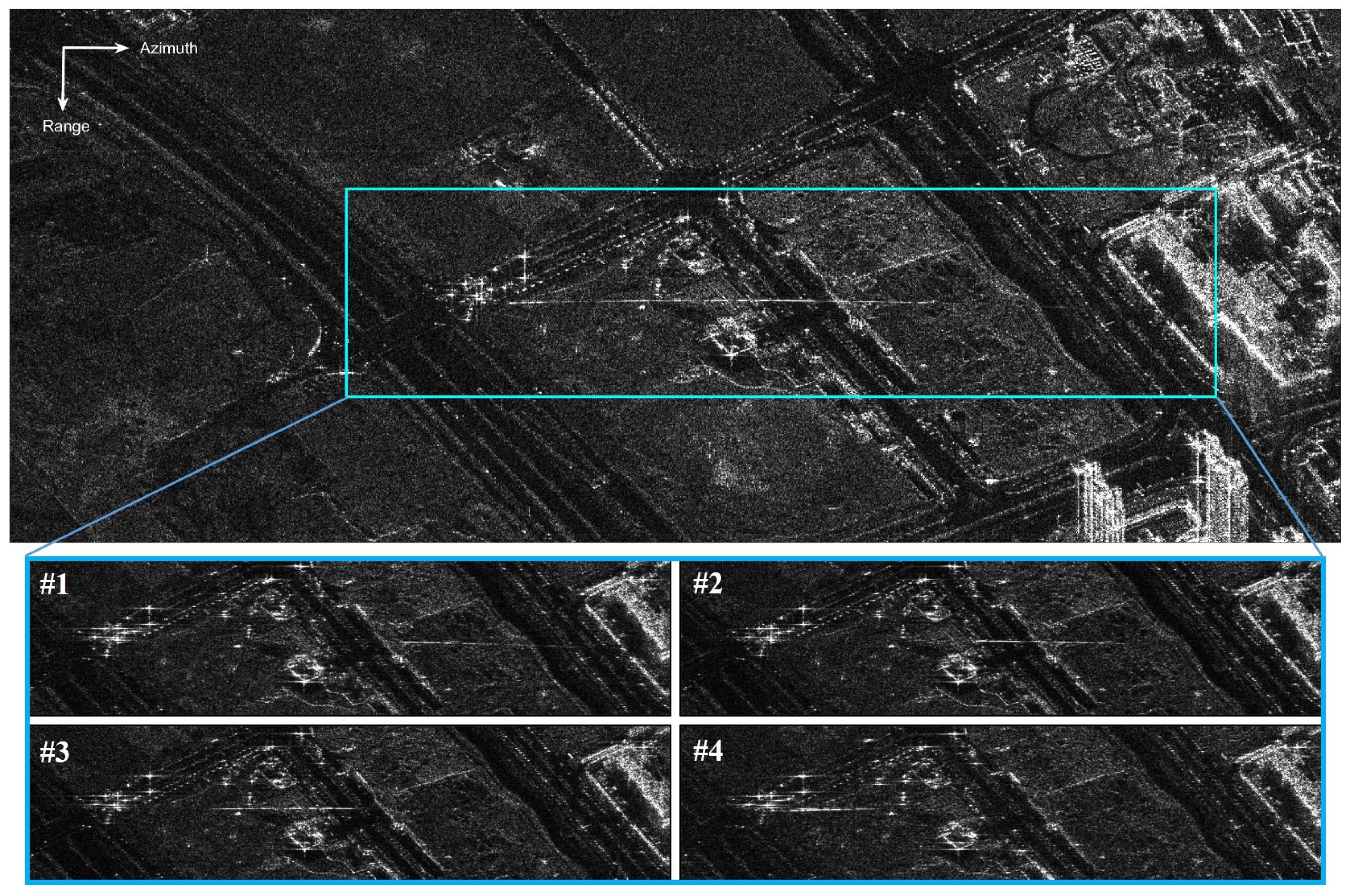
The SLC image to be processed is collected in spotlight mode over Nanjing city, China, 2017. The related parameters are listed in Table 1. A small region in SLC image is processed to demonstrate the proposed method. The corresponding SAR image is shown in Figure 1 upper figure. The horizontal and vertical directions are the azimuth and range respectively. A moving target signature can be seen as denoted by the blue box. The target’s image trace spans around 430 m along azimuth direction. To show the motion of moving target’s signature, four subaperture images of the area bounded by the blue box are generated as shown in bottom of Figure 1. According to four images, it is clear that the moving target signature moves from right to left. The goal of this paper is to use the proposed method to detect the moving target.
3. Signal Model
The shape of moving target signature in the SAR image is important for the image sequence-based detection method. In this section, we give the analytical expressions of a moving target’s image trace. The analysis shows the azimuth length of target’s image trace can be used to estimate the coarse azimuth speed. Then, we use the expressions to analyze the characteristics of image trace with Gaofen-3 spotlight SAR parameters (listed in Table 1). The analysis can also demonstrate the feasibility of the image sequence-based detection method.
Some interesting studies about a moving target image trace have been reported. Jao deduced the functions of constant speed target’s image trace in linear trajectory SAR [14]. It has shown that its shape is an elliptic or hyperbolic curve. In [15], Chapman analyzed the indistinguishable problem between moving target and stationary target signature. He points out that image sequence-based detection suits spaceborne condition for linear trajectory SAR, since the platform’s high speed limits the happening of indistinguishable problem. Here, we adopt the method [16] which was proposed by our team to conduct the analysis.
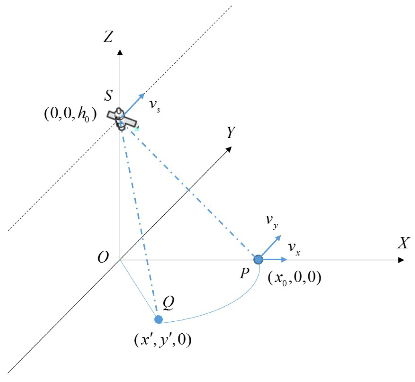
The SAR satellite’s orbital trajectory is usually defined by the parameters of orbital elements. However, since the Gaofen-3’s observation time (12.5 s) and aspect angle () are small, the linear trajectory is sufficient for the deduction. In addition, the flat earth is assumed for deduction convenience. For moving target, the simple constant speed motion is analyzed. The acquisition geometry at time is shown in Figure 2. X and Y axes are range and azimuth direction respectively. is the ground plane. The SAR sensor(denoted as S) moves along Y direction at height with velocity . A constant speed target P moves in ground plane with velocity . Because of symmetry reason, the target is characterized as lying on the X axis when . The target/SAR motion functions are listed in Table 2.
is the target’s image position. According to [16], the image position B can be computed via Range-Doppler(R-D) equations. The R-D equations are
The first equation is a Doppler expression which is first order. It means that the Doppler from Q is equal to the Doppler from P subtracts the target’s motion induced Doppler. The second one is the Range equation which means that the P and Q lie on isorange line. Replacing the motion functions into the Doppler equation in (1), we can obtain target’s image position as (2).
The is the target azimuth image position which can be calculated via Doppler equation in (1) directly. The second line is the cross track position which is computed by combining the range relation and the . is the relative speed. Because the proposed method utilizes the defocusing effect in along track, the analysis focuses on expression . One more thing should be noted, here, the image trace functions correspond to the peak positions (ridge) of the moving target signature in a SAR image.
From first line of (2), the is a linear equation. The second term is the azimuth offset caused by the range speed which corresponds with the analysis in [17]. The azimuth offset is zero when target has no range speed, which means target lies on its real position. The first term can be interpreted as the target’s azimuth image speed , which is controlled by the square of relative speed . It is quiet interesting to find that target’s azimuth image speed is constant value and the target’s real heading angle has no influence on it. Another interesting thing is that the moving target is focused when . The corresponding deduced results are shown in (3)
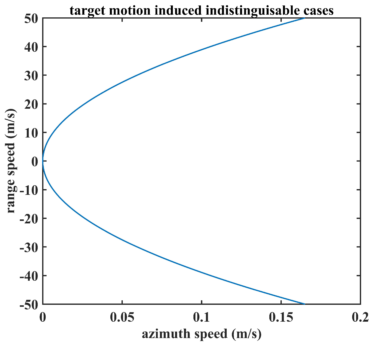
The target image position becomes a constant value which means it can not be distinguished from a stationary point target. In such case, the moving target can not be detected theoretically. However, considering the point target and ideal constant speed assumptions, there is little chance that it would happen in a real scenario. To further demonstrate that, the motions in Gaofen-3 are computed via and plotted in Figure 3. From Figure 3; the range speed contributes more to such cases than azimuth speed. For typical along speed interval like 5~30 m/s, the required range speed would be unrealistic. Since the method only focuses on those targets with relatively high azimuth speed, such cases will not be a problem.
The proposed method requires a target’s long smear trace in SAR image along azimuth direction, thus, azimuth image speed is important. We further analyze which speed component of the target motion dominates the azimuth image speed. Replacing the into to obtain (4).
Consider the and in spaceborne case, the (4) can be approximated as
From (5), the is dominated by azimuth speed . High azimuth speed is preferable for the image sequence-based detection method.
Furthermore, multiply observation time on both sides, we can get the length of a target’s signature along azimuth is 2 times of its real azimuth travel distance as shown in (6). Using this relation, we can obtain the coarse estimation of target azimuth speed component .
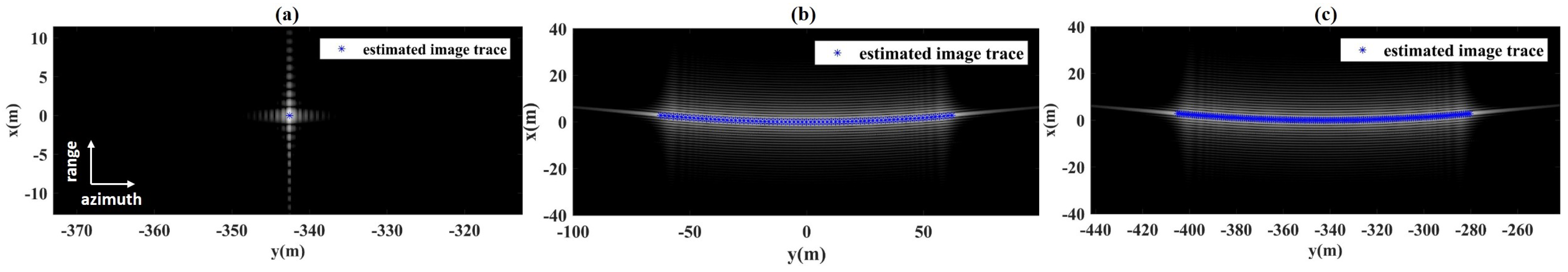
In order to validate deduced target image position functions, the point target simulations are conducted. The parameters of Gaofen-3 in Table 1 are used in the simulation. Three moving targets A,B,C are considered. Their motion parameters are given in Table 3. The first two targets are set to show the shapes when the target only has azimuth or range speed. Target C has both range and azimuth speed, and the azimuth speed is equal to target B. The purpose of these two targets is to demonstrate that the target’s azimuth smearing lengths are equal when they have same azimuth speed. After SAR processing, the images of three targets are shown in Figure 4. The blue ′*′ denotes the predicted image trace using (2).
The Figure 4a shows the signature when target moves in range direction. The target shifts in azimuth and has no defocusing effect, which corresponds to the above analysis that the azimuth speed component controls the smearing. The computed target image trace matches the SAR signature, which means the deduced functions are effective. The subfigure (b) is SAR image of target only has azimuth speed. The signature stretches in azimuth, which demonstrates the smearing effect is caused by the azimuth speed. Plus, since the target has no range speed, the azimuth shift offset is zero as the center of target signature lies on in the subfigure (b). Moreover, the target real azimuth travel distance is 62.5 m, and the azimuth smearing length is around 120 m in SAR image which is two times of real azimuth travel distance as expected. The computed image trace matches the signature shows the effective of deduced functions for azimuth moving target. To evaluate estimation performance for general moving target, target C is selected. From the figure, its signature is almost identical to target B, and again the computed image trace matches the target signature. Here, it should be noted that two times relation between target signature and azimuth real travel distance shows again, which proves that the smearing length is not influenced by the target heading angle.
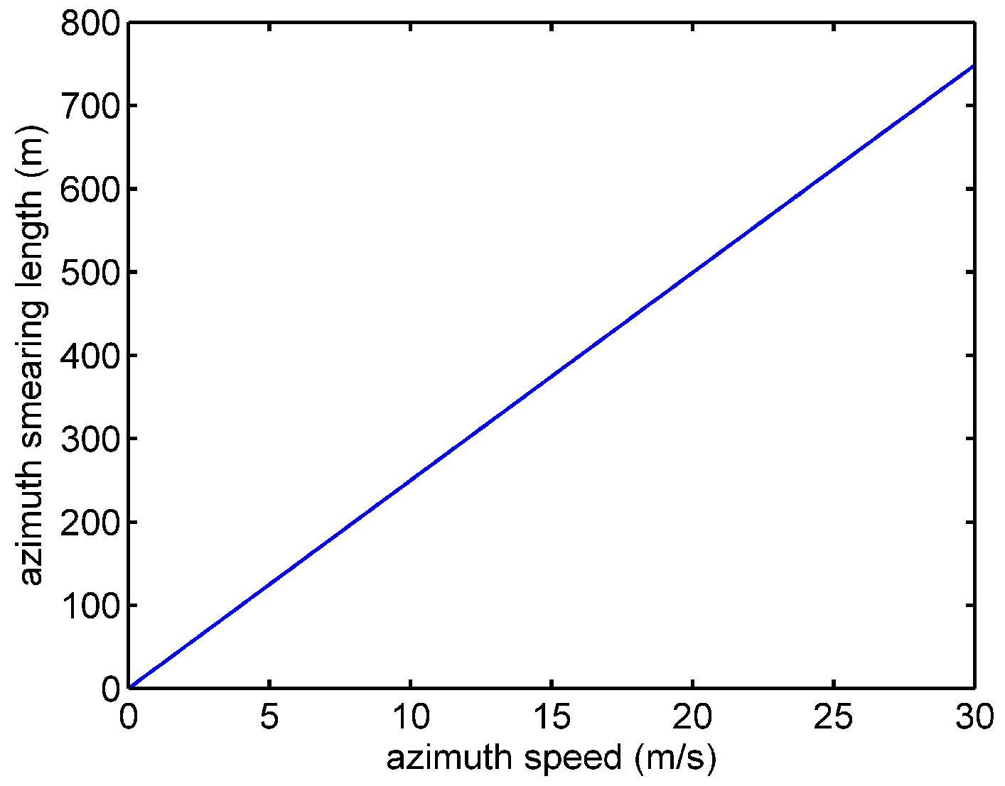
After proving the effectiveness of deduced image trace functions, the curve of target’s azimuth smearing length in versus azimuth speed is plotted in Figure 5. From the figure we can see, the higher the azimuth speed is, longer the azimuth smearing length will be in SAR image. During 12.5 s illuminating interval, even with 5 m/s azimuth speed, the output length is beyond 100 m. It indicates the spotlight mode is sensitive to the azimuth slow moving target. The long smearing trace is good for image sequence-based detection method since longer the smearing signature, the more subaperture images we can obtain. The feasibility is therefore demonstrated.
4. Method
In this section, the proposed method is described in detail.
The background subtraction method is first developed and successfully applied in the optical video surveillance domain [18,19], a logarithm kind method can be found in [20], but such an idea is first introduced in SAR moving target detection by our team (to our knowledge) [11]. The main idea of the logarithm background subtraction method is simple. It regards the original SAR image as the combination of the background image (static scene) and foreground image (moving target). On one hand, because the azimuth viewing angle of spaceborne spotlight SAR is small as in the Gaofen-3 system, the static scene presents less anisotropic scattering behavior, and its pixel values are relatively stable in subaperture images. On the other hand, the moving target signal’s image position changes from subaperture image to subaperture image. Therefore the background image can be generated with the subaperture image sequence. Then, the static clutter can be removed by performing logarithm subtraction process. The logarithm subtraction process is designed by integrating the log-ratio operator [21] which is robust and is widely used in SAR change detection applications to obtain good clutter suppressing performance. The target signals is then easier to be detected in the foreground images.
However, the target SNR is relatively low in spaceborne SAR, thus, the three levels detection is designed in proposed method to handle the issue. The first level is to apply a low threshold CFAR detector to the subtraction result, so that most of the moving target signatures can be well persevered. The output also has high false alarm. To reduce the high false alarm in the first level detection result, the modified DBSCAN clustering method is applied. The moving target signature has high density (occupies connected pixels), while the false detection has low density. The last level utilizes the false detection’s random moving behavior in image sequence to exclude the remaining false detections, since the moving target signature has dynamic behavior.
4.1. Processing Chain
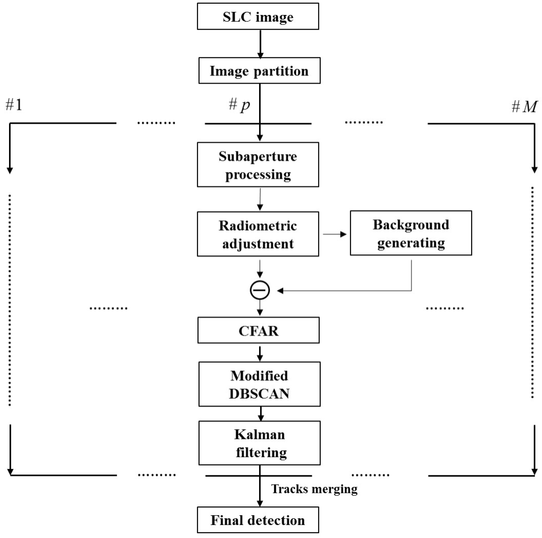
The flow chart of the proposed method is shown in Figure 6. The algorithm consists of the following steps: (1) Input the SLC spotlight SAR image; (2) Partition the SLC image into M patches. (3) For p patch, generate the overlapped subaperture image sequence via subaperture processing. All subaperture images are indexed with corresponding azimuth viewing angel. Suppress the speckle noise and transform the image sequence into dB unit to get the Overlapped Subaperture Logarithm Image (OSLI) sequence; (4) Apply radiometric adjustment to the OSLI sequence to suppress the antenna illuminating effect; (5) Apply the median filter to the OSLI sequence along the third dimension (corresponding to the azimuth viewing angle) to generate the background image; (6) Use the radiometric adjusted OSLI sequence to subtract the background image; (7) Apply the CFAR detector on each image to get a set of binary image results; (8) Cluster the potential moving target by performing the modified DBSCAN on each binary image; (9) Input the clustered potential targets to the Kalman tracker to obtain the detected moving targets’ track from patch p; (10) Merge the tracks from all M patches as the final detection output.
The main processing steps are from subaperture processing to Kalman filtering, their detail is introduced as follows.
4.2. Subaperture Processing
After partition the image into several patches, the first step is to generate the OSLI sequence. To make sure the algorithm works, a proper OSLI image sequence should meet three requirements. First, each image should have the same resolution. Because the static scene is assumed to be changed little, the resolution difference in part of the image deteriorates the quality of the background image and then the detection results. Second, filtering the background needs the image sequence share the same geometry. Thus, the image coregistration is required. The last one is that the images in the sequence should be overlapped. Because of the target signal occupies mutual pixels in overlapped image sequence. It is good for target tracking in the last step. It also helps in increasing the number of the images in the sequence so that the robustness of background generation step is improved.
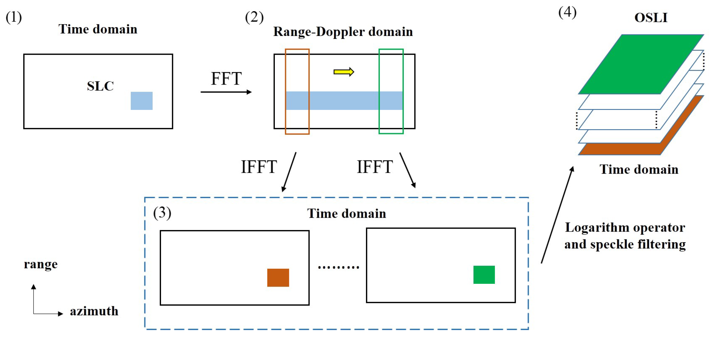
As mentioned in the previous section, a spotlight SAR SLC image is the input material. Using the SLC image increases feasibility of the algorithm. In addition, the above requirements can be fulfilled easily. Because each patch contains all its azimuth information, cutting its signal in the range-Doppler domain will only generate a subaperture image of this patch. The same resolution and overlap requirement are also guaranteed by implementing a fixed sliding window when cutting the azimuth spectrum. The illustration of subaperture processing is shown in Figure 7. In practical implementation, the proposed algorithm processes the SLC patch by patch. Thus, we set the rest of the data as zero so that the original image spacing is retained. Then, we apply the FFT along azimuth. Next, a fixed sliding window will cut the signal’s spectrum to obtain N segmentations of the signal corresponding to the different Doppler. After applying the IFFT on each split azimuth spectrum, we can get N overlapped images. Considering the small angle approximation in the Doppler formula in (7)
Each image corresponds to a look angle , the images are denoted as . Apply the logarithm operator (each is expressed with dB unit) and speckle filtering, the OSLI sequence is obtained by indexing the images with look angle . The expression of OSLI is denoted as
During the process, the azimuth size of the sliding window (it controls the segmented bandwidth of subaperture image) and the overlap rate between adjacent images is key parameters in algorithm.
For the first parameter, the main considerations are SNR and resolution. In a large bandwidth case, the energy of static clutter is accumulated, but it does not work for the moving target signal, because of the smearing effect. Part or whole of the moving target signal may be masked by the clutter in such conditions, which degrades algorithm performance. In the small bandwidth case, the target SNR can be improved since the smearing effect is mitigated. Thus, a small bandwidth is suggested when implementing the method. The quantitative analysis of optimal bandwidth for subaperture image generation is now being studied.
As for the overlap rate, since the spaceborne SAR has little azimuth spectrum information compared with airborne SAR such as circular SAR, the high overlap rate can provide more images which is good for the background image generating step. Hence, a high overlap rate is recommended.
4.3. Radiometric Adjustment
The second processing step is the radiometric adjustment. Because the algorithm assumes the pixel value is only azimuth viewing angle-dependent, the weight caused by the antenna illumination variation need to be removed. The optimal solution is to remove the antenna pattern when knowing its 2D information. Since we do not have such data, we apply an image processing method called intensity normalization [22] to deal with it.
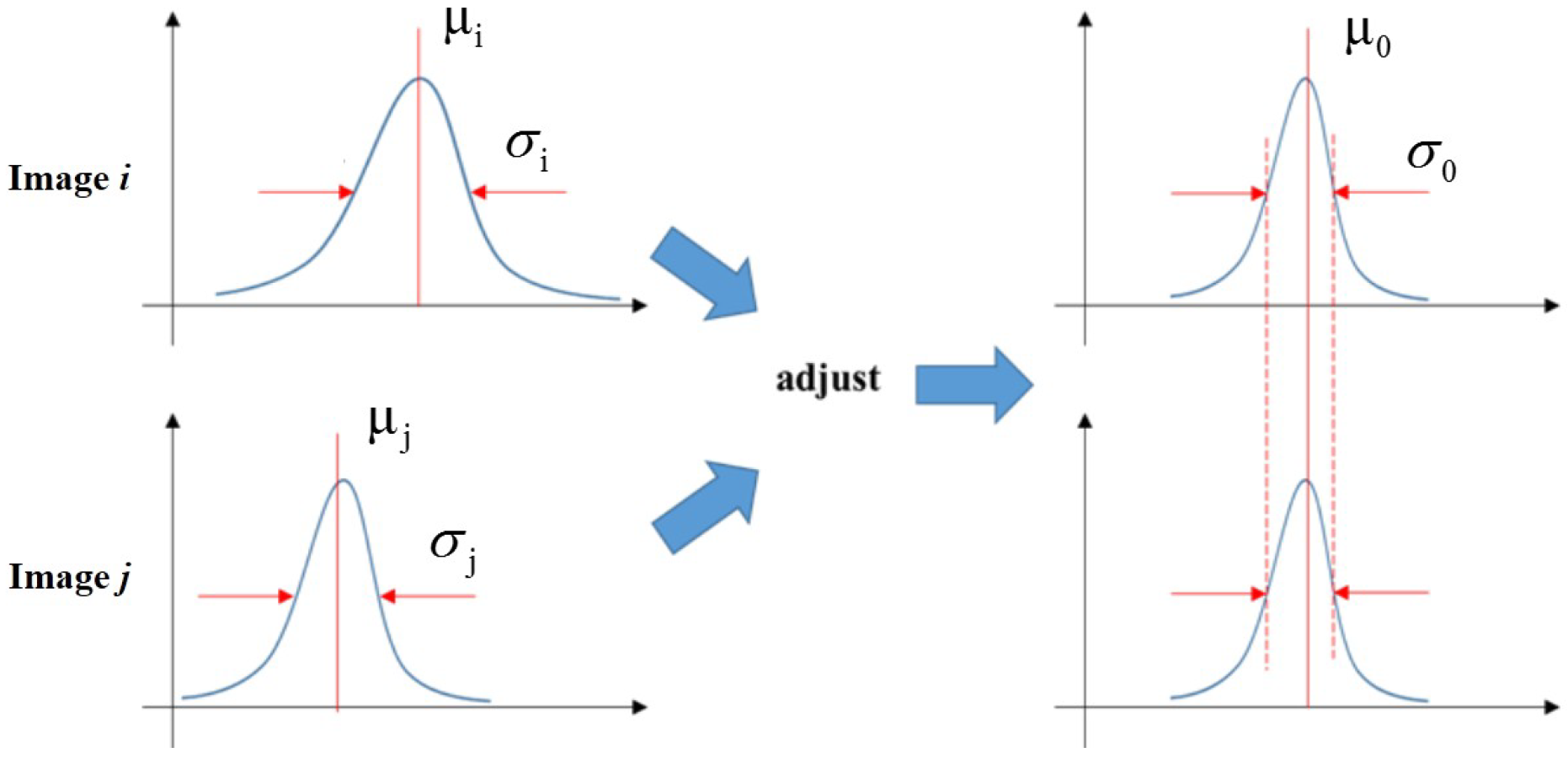
Figure 8 shows the illustration of the intensity normalization. This method adjusts the image statistic of all images to the common value. We first collect all mean and standard deviation of the histogram from each image in OSLI sequence. The corresponding expressions are shown as (9).
E means expectation in (9). Then we calculate their mean values as the common value by (10).
Using the common values to adjust each image in OSLI as (11).
The adjusted OSLI which denoted as can be used for background generation step.
4.4. Background Image Generating and Subtraction
The idea of generating a background image is simple. As mentioned above, the basic assumption is that certain pixel values change slowly along the azimuth viewing angle. With coregistered and radiometric adjusted OSLI, we obtain the curves of pixel values. The position of moving target signature changes relatively fast from image to image. Thus, for a certain pixel, a high value will occur when the moving target signature moves onto it. It is a straightforward thinking to detect this anomaly in the each pixel’s changing curve as [10]. However, different types of static clutter (like anisotropic and isotropic types) present different azimuth backscatter behavior as reported in [23], and thus, makes the uniform threshold hard to be determined. An alternative plan is to use the subaperture image sequence to generate the background image.
We apply the median filter to the each pixel’s changing curve, and select the median value to represent the background. Thus, excluding the high value caused by the moving target signature. In practical, this can be done by applying the median filter to the OSLI along the dimension. The corresponding expression of background image is (12).
is the output background image. Because the image in OSLI is expressed with dB unit, the background image is also in dB unit and adopted with similar notation.
After generate the background image, the foreground image sequence can be obtained via (13).
In (13), the represents subtraction result of ith image in OSLI sequence. Since the background image and the image in OSLI are all expressed in dB unit, the subtraction process is equal to the ratio process. Due to the subtraction process, the unchanged parts (static clutter) in OSLI are gathered around zero in histogram of , while the changed parts(moving target signal) are persevered and fall into the tail of the histogram of . Compare the conventional log-ratio operator in reference [24], expression (13) has the same form. Log-ratio operator is widely used in change detection applications, and the Gaussian distribution is suggested for modeling the ratio image as in [24]. In addition, paper [11] used the real data to prove the effectiveness of modeling the foreground image with this distribution.
The quality of the background image has serious influence on the performance of subsequent steps. Since the following CFAR, modified DBSCAN and Kalman filtering steps are based on the assumption that the moving target signature is persevered and the static scene is subtracted after the background generation and subtraction step. If the filtered background still contains the target signature or its residual signal, the performance of background generation and subtraction will be degraded. From this view, the influence of parameter the number of images (otherwise the aperture length) on background generation and subtraction is investigated in experiment section. It is shown that when more images (aperture length) are used, the better the performance of background generation and subtraction will be.
Since the background image is composed of median values, there is residual clutter in the subtraction results. Considering the Gaussian distribution is effective for modeling the foreground image’s histogram, it is convenient to apply a CFAR detector to detect the moving target signal as the first level of detection in the proposed algorithm.
4.5. CFAR Detection
A conventional two parameter CFAR detector is selected as the first level detector [25]. Due to low SNR in spaceborne SAR image compared with airborne case, the influence of speckle noise and residual clutter is much severe as will be shown in the experiment. Thus, the purpose of this CFAR detector is to provide a coarse detection results. Thus, the false alarm rate is set relatively high, in another word low threshold, so that most of the target signatures can be preserved. The false alarm is reduced by the next two steps.
A CFAR detector is applied using a sliding window centered around the test cell as depicted in Figure 9. The data of background ring is used for estimating the parameter (mean and standard deviation ) of Gaussian distribution. The expression is given as:
It is convenient to make the substitution of to get the normal distribution . As in last subsection, the residual clutter(unchanged part) is around zero in histogram while the moving target fall into the tail part. We assume that thebackground image only contains the static clutter and a high value occurs when the pixel contains moving target signature, thus the target signature will contribute to the positive part of the histogram. Then, the threshold is calculated via (15)
is the false alarm we set. Hence the decision rule for test cell is:
The expression of first level detection results is given as (17)
After the CFAR detector, the morphological closing process is recommended. In the subaperture process step, the small segmented azimuth bandwidth is applied to guarantee the partial or whole moving target signal woould not be masked by the clutter. However, the background image consists of a median value; the value of moving target signal in subtraction result may be partially lower than the CFAR threshold, i.e., the detected moving target signal may be broken after CFAR. The morphological closing can erode those small size false detections and fill the gap between the adjacent broken moving target signatures. In practice, the parameters of morphological closing should be selected carefully so that the false detection which occupies many pixels may be falsely connected. The parameters are chosen so that the one pixel false detection is eliminated. As for those broken moving target signatures which may not be connected by the morphological closing process, the clustering step is selected to deal with this issue.
4.6. Modified DBSCAN
The second level is to use the clustering algorithm to reduce the false alarm. Because the CFAR results are the binary images, the detected target can not be used for applications like speed estimation and direct refocusing. Thus, the clustering step is essential, and the parameters (such as centroid and length) of clustered moving target candidates can be used for the Kalman filtering in the last step. Furthermore, the broken moving signature problem can be solved easily by utilizing the clustering method. Instead of connecting the broken signature, classify those broken signatures as a cluster which is rather an efficient way. Plus, the features of the cluster like centroid also work for next step of Kalman filtering.
Among numerous algorithms, the DBSCAN method [26] is selected because of several advantages. First, DBSCAN can find arbitrarily shaped clusters. Most importantly is that it does not need to specify the number of clusters, compared with the k-means method [27]. Because the number of moving targets is unknown typically, it makes this method well suited for the task. Second, the residual clutter and noise are distributed randomly in foreground images while the moving target signature covers an unbroken area. The false and right detections after CFAR processing also have this feature and, hence, makes the density-based method DBSCAN a good choice.
To apply conventional DBSCAN on the coarse detection result (binary image) needs two parameters to form a cluster: Eps and MinPts. The Eps represents the neighbor radius of a given pixel. MinPts is the minimum number of pixels needed to compose a cluster, i.e., the density threshold. As shown in Figure 10a, the red part denotes the moving target signature and the blue pixels denote the false detections. Since the moving target signal is defocusing along azimuth and, hence, presents as line shaped signature, we apply the conventional method directly on the binary image and we may classify the adjacent false detection as part of a moving target candidate. To solve this problem, we use a rectangle rather than a circle to perform the clustering. Figure 10b illustrates the modified DBSCAN. The length of rectangle along range and azimuth direction are and . The two parameters and Minpts need to be tuned to get good clustering performance. So far the parameters are set according to experience.
The algorithm begins searching pixels randomly, if there are more than Minpts pixels within the rectangle area, these pixels can form a cluster. Those pixels which do not fulfill above condition are labeled with noise. A search and find operation is conducted for all pixels until all pixels are classified in a certain cluster or as noise. We apply this algorithm to each binary image in the CFAR output to obtain the moving target candidates. The output of the second level detection results is
refers to modified DBSCAN. After get the clusters, their centroid and minimal bounding box are extracted for the next Kalman filtering step. The centroid is denoted with , x and y are the range and azimuth direction respectively. The minimal bounding box A is composed of four variables . and are the position of top left point, and are the size of the box.
4.7. Kalman Filtering
Although the modified DBSCAN can further reduce the false alarm and obtain the moving target candidates, the performance of DBSCAN is decreased when the different densities exist. Furthermore, the clutter’s anisotropic scattering behavior and rotating sidelobe may be preserved through the subtraction to the modified DBSCAN processes. Thus, we exploit the moving target’s dynamic behavior in the SAR image sequence to get the final detection results. For Gaofen-3 SAR staring spotlight mode, the observation time is s. During this period, constant acceleration model is a good approximation for modeling the moving target’s motion. And as analyzed in previous section, the target signature presents the linear motion along the azimuth in OSLI. Thus, the traditional Kalman tracker is OK to handle this step [28].
We assume K clusters in are the moving targets. Set their centroid as the start of the track , and its minimal bounding box is also restored in . By applying the Kalman filtering from to , we can get whole tracks. Since the moving target signature moves along azimuth direction with approximately linear motion, while the motion of false detection is random. Thus, the wrong tracks can be excluded, the tracks correspond to the right motion are preserved as the output final detection results.
The state of the system as all the states of each cluster is defined as . These , are the target speed and acceleration along corresponding direction. We use the Kalman filter to predict th state of the system for image . The predicted state is . To find which cluster in the should be assigned to the track , the y direction distance of the centroid and the overlap rate of the minimal bounding box are computed. The recorded ith minimal bounding box in and predicted th centroid are and . The overlap rate between the and the clusters in is shown as
Because the OSLI is overlapped, the moving target signatures are also overlapped. Therefore, the right cluster which can be assigned to the track should meet . We then use the y direction distance to further exclude the wrong clusters, since there might be more than one cluster that can fulfill the condition. The y direction distance between the predicted centroid and the clusters in is given as
consists of two parts, first one the absolute value of the y direction distance. The second part is which is to make sure the assigned target moves in azimuth direction. is the assignment threshold. Then, the cluster which corresponds to the shortest distance is assigned to the track using the information of the assigned cluster to update the Kalman filter and perform the above procedure iteratively until .
However, certain tracks should not to be assigned when several cases happen. First, when the tracked moving target moves out of the scene; second, the certain track is not assigned a cluster more than 3 times (this threshold is obtained by experimental testing). The algorithm is processed patch by patch, thus, we merge the tracks that pass through the azimuth adjacent patch. After we obtain all the tracks, we apply a threshold to get the final detection results. The corresponding expression is given as
The left side (21) denotes the azimuth length of track , while the right side is the threshold. Then those tracks whose azimuth length is lower than the threshold will be excluded. As in the previous signal model section, the azimuth length of target signature is two times of its real azimuth travel distance, i.e., the relates to the target azimuth speed. In another words, the threshold can be set by considering the target’s minimal azimuth speed we want to detect.
5. Experiment
5.1. Processing Results
In order to validate the proposed method, the detail of processing selected Gaofen-3 data (as shown in Figure 1) is presented.
The selected scene is part of the original SLC image, and a moving target signature can be seen clearly. The selected scene does not need to be partitioned, the first step is then subaperture processing. As in the previous section, the small bandwidth is recommended for subaperture processing. Here, the azimuth size of sliding window is 2000 pixels corresponds to the bandwidth of 1495.4 Hz (the original azimuth processing bandwidth is 19,379.69 Hz). The azimuth resolution is reduced from 0.33 to 4.25 m. The overlap rate is set as , which means that the sliding window forms a subaperture image every 200 pixels. The generated image sequence consists of 100 images. Transform the image sequence into dB unit and apply average window to reduce the speckle noise. Then, index the images to get the OSLI sequence.
The original logarithm background subtraction algorithm is developed for the airborne circular SAR mode which has plentiful angular information ( typically). However, Gaofen-3 staring spotlight mode’s azimuth observation angle is only , thus, the whole OSLI (contains 100 images) is used in the following experiment. It will be demonstrated that the good quality of background image and subtraction performance can be achieved by using 100 image. Here, the 18th image is chosen as the example for the demonstration of each step, the image is shown in Figure 11a.
Next is to apply the radiometric adjustment on acquired OSLI sequence. According to (10), the obtained common values are and . Then, using (11) to adjust the histogram of images in OSLI. Figure 12 shows results of 18th and 68th image before and after applying intensity normalization. The red line and green line in images denote the mean value and standard deviation. The first column is histograms of two images before applying intensity normalization. From the subfigures, the mean value and standard deviation of 18th and 68th are not equal. After applying the method, the corresponding parameters are equal as shown in the right side column. Apply this process to all the images in the OSLI to reduce the antenna illumination effect, then generate the corresponding background image with the adjusted OSLI.
In the beginning of this section, the whole OSLI sequence (100 images) is used for the experiment. There are two reasons. First, since the Gaofen-3 has less angular information compared with airborne CSAR, the anisotropic feature are not evident which meet the slowly varying assumption mentioned in Section 4.4. The other one is that the generated background image has better quality if more images are used. This can be found in reference [11]. The generated background image is shown in Figure 11b. Compare Figure 11b and a, it is clear that the moving target in subaperture image is filtered in the background image. Furthermore, the other parts of the signature in the original SLC image are also filtered, thus, validating the effectiveness of the background generation step.
Then, the clutter can be suppressed via the subtraction process. The modified logarithm background subtraction algorithm integrates the log-ratio operator which is widely used in change detection applications to achieve good performance in suppressing the clutter. From the foreground image shown in Figure 11c, the clutter (i.e., static scene) is well suppressed. The right side building structures and left side road are all subtracted. The moving target signature is quiet evident in the subfigure (c), while the rest area looks homogeneous which is very good for target detection.
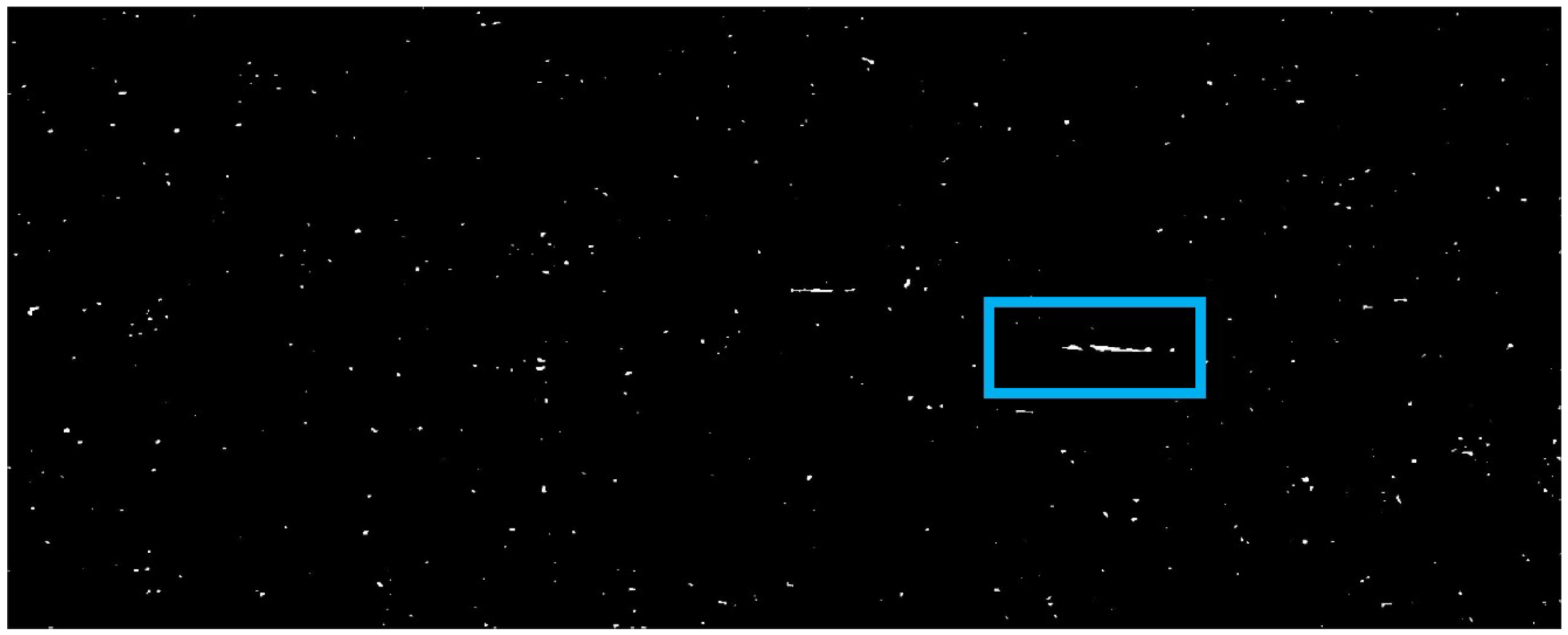
As mentioned, the Gaussian distribution is adopted to characterize the statistical distribution of foreground image. The foreground image’s histogram is shown in Figure 13. The red line is the fitted Gaussian distribution, and it is evident that the histogram matches the distribution. Then, the CFAR detector is applied. The false alarm rate (PFA) is 0.27, so the corresponding low threshold can preserve most of the target signature. The size of CFAR window is , and for the test region. Figure 14 shows result of 18th image after CFAR detection and morphological closing operation. We can see the shape of detected target matches the shape in foreground image. Moreover, a lot of false detections and target signal broken phenomena are as the previous analysis. In Figure 14, we can see target signature presents high density while the false detections are not. Hence, provide the basis for applying the modified DBSCAN to further exclude the false detections.
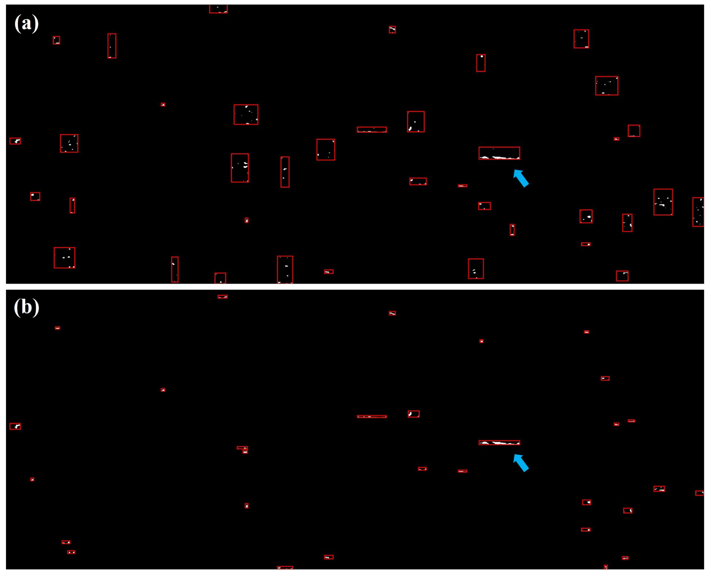
To implement the modified DBSCAN algorithm, three parameters are required: size of rectangle and density threshold MinPts. The size of the rectangle is pixels and pixels, the MinPts is 40. These empirical parameters are acquired by testing, their effectiveness are validated with both experiment results and performance analysis. The optimal parameter and automatic parameter selection is part of further work. To demonstrate the modified DBSCAN method and make a comparison with the conventional DBSCAN method, we apply them to the 18th binary image. The results are shown in Figure 15. The Figure 15a,b are results of the conventional method and the proposed method, respectively. Each cluster is denoted with a rectangle using the minimal bounding box parameter. The arrow points to the moving target signature. From (a) and (b), we can see the target signature in two images are both broken, but the broken parts are well classified as one cluster as expected. Moreover, compared with CFAR result in Figure 14, those low density false detections are excluded in Figure 15a,b. However, comparing (a) and (b), although the real moving target signature in two images are all classified as one cluster, the minimal bounding box in (a) is larger than the box in (b). It means that the adjacent false detections and real moving target signature are falsely classified by conventional method, which matches the previous analysis. From (b), we can find that this disadvantage is avoided by the modified DBSCAN method. In addition, we can also see that the conventional method has more falsely classified clusters. Thus, the comparison proves that the modified DBSCAN method is better than conventional method when classifying moving target signature. The modified DBSCAN is, therefore, demonstrated.
Then we evaluate influence of the parameters and Minpts on the modified DBSCAN’s performance. The modified DBSCAN has two goals, the first is to cluster the broken signature as one cluster, the second one is to reduce the false alarm. Because the moving target signature defocuses along azimuth direction rather than range direction, the and Minpts play key roles in this step. For convenience, the Minpts is expressed with ratio of Minpts to pixels of sliding window to suit different . We characterize performance with two factors: the clustering accuracy on real target signature and the false alarm rate.
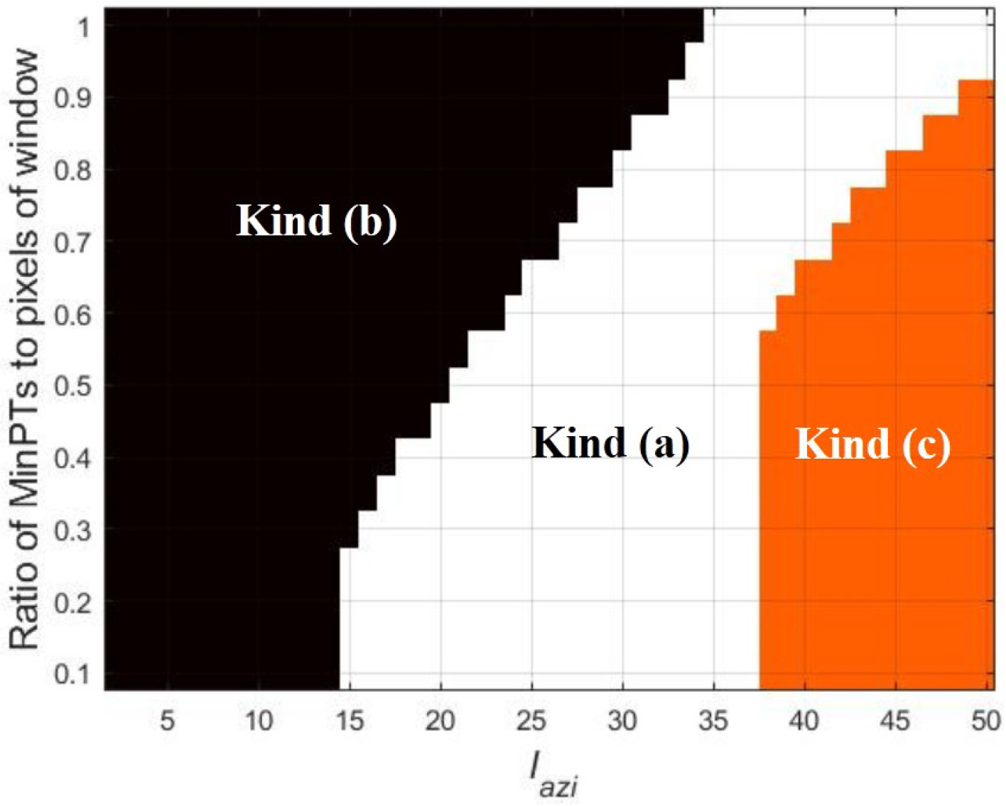
First, we use the 18th image Figure 14 to get the clustering accuracy, and the real moving target signature is labeled manually as the truth data. Because the target signature is broken and surrounded by the false detections. Thus, the results of clustering accuracy have three kinds:
- (a) the real target signatures are classified as one cluster (correct);
- (b) the real target signatures are classified as different clusters (incorrect);
- (c) the real and false target signatures are classified as one cluster (incorrect);
Apply the modified DBSCAN to the 18th image with different and , and compare with the truth data to obtain the clustering accuracy. The result is shown below.
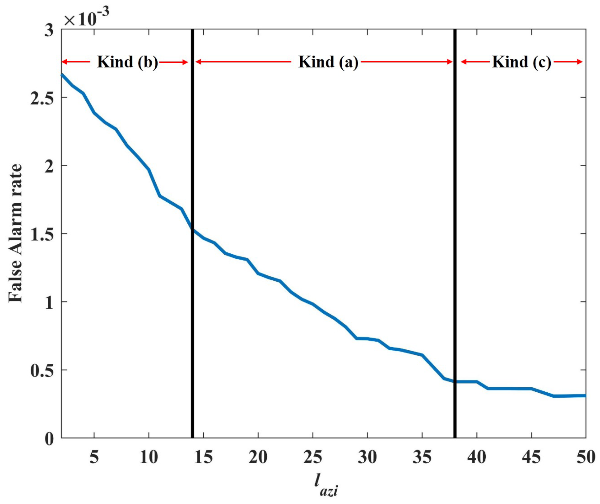
In Figure 16, the black part and orange part are the wrong classifications, kind (b) and kind (c), respectively. The white part denotes the right classification kind (a). It is clear that real target signature can not be correctly clustered when , partly corrected clustered for . For , the target can be corrected classified for all . The selected parameters , , (i.e., ) lie in this interval, which shows the effectiveness of the parameters. Since for all , the target can always be correctly clustered when , the false alarm rate versus when is analyzed. The result is shown as Figure 17.
The false alarm rate is defined as the number of clusters per square kilometer. We can see that the false alarm reduces when increasing the . The curve is divided into three parts according to the clustering accuracy. When and , the real target signature can not be correctly clustered. Thus the effective interval for lies on . In addition, is in this interval, its false alarm rate is 6.08 × which almost reach the minimal value. Thus, the parameters for the experiment are sufficient.
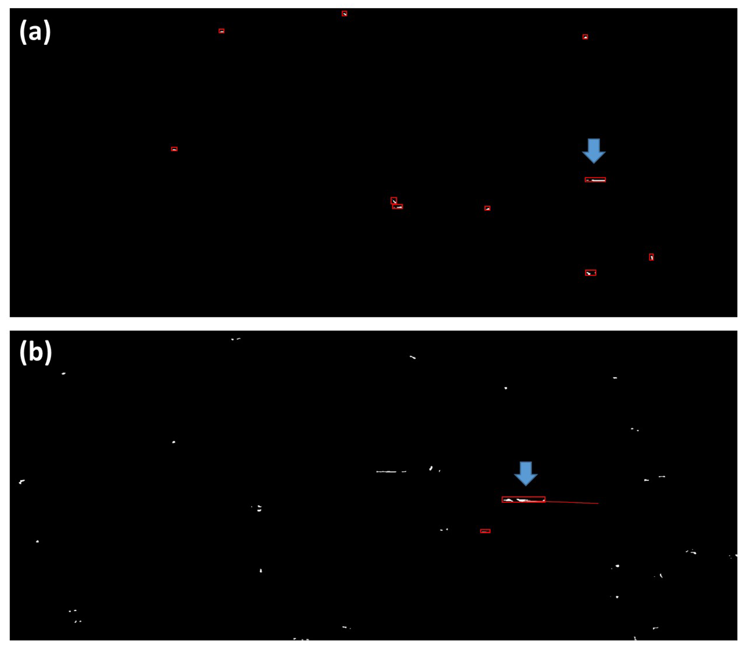
After applying modified DBSCAN, the residual false detections are eliminated by utilizing the true target’s dynamic behavior. Apply the Kalman tracker to the first image, then using the clustering results to update the tracks iteratively. 10 clusters are obtained in first clustered image, thus there are 10 tracks being initialized as shown in Figure 18a. Blue arrow denotes the moving target. The clusters correspond to the tracks are labeled with red rectangles according to the parameter of minimal bonding box.
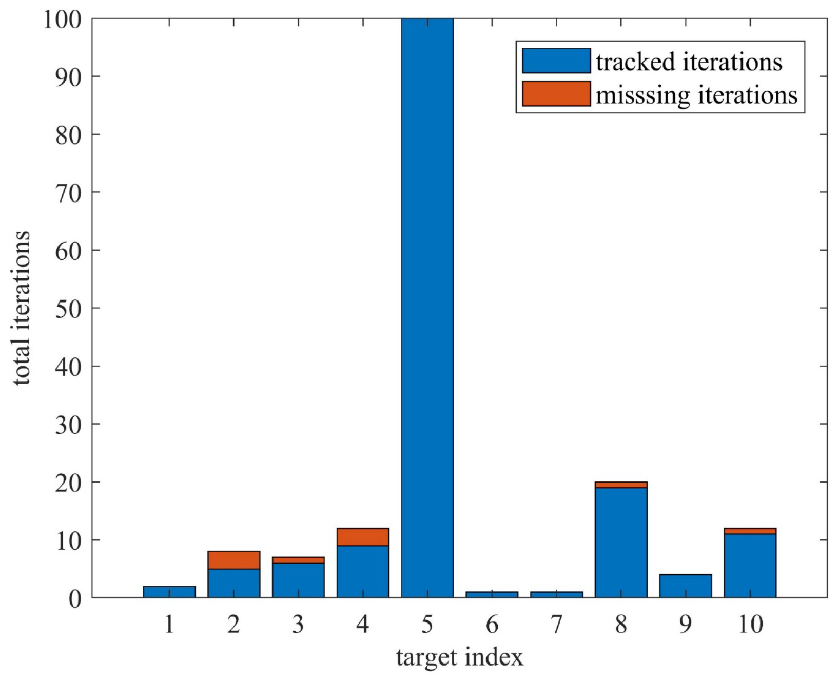
The tracking results in the corresponding 18th clustered image are shown in Figure 18b. Compared with subfigure (a), there are only two tracks still updating. The tracks correspond to the false detections in the first image can be regarded as being excluded. The blue arrow denotes the tracked moving target signature. The red line denotes its moving trace, which shows the good linear moving behavior as analyzed in the previous section. Here, the reader can also notice that the remaining false detection lies on the lower left of the moving target. Although it is tracked in 18 iterations, its trace lies within the current minimal bounding box. After running 100 iterations, we find the update of this false track stops at 20 iteration. Because the false detections appear randomly in images, the false detections do not have dynamic behavior as real moving target signatures. The overall tracked iterations and missing iterations of ten tracks are shown as Figure 19.
The blue and orange part correspond to tracked iterations and missing iterations, respectively. The 5th track is a real moving target, which shows it is tracked in 100 iterations without missing. The rest of the tracks correspond to the false detections stop updating after 20 iterations. We collect the maximal azimuth moving distance of ten tracks, and compute the corresponding azimuth speed according to (5). Table 4 shows the results. According to (21), we set the 100 m as the threshold. Then, the final result is just the 5th track.
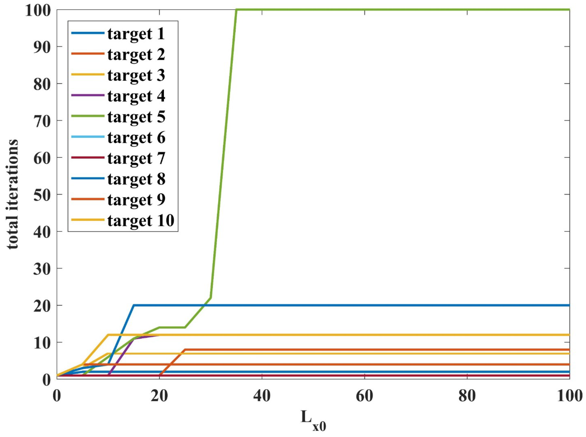
In Kalman filtering step, the important parameter is assignment threshold in (20), since it determines whether a cluster will be assigned to the certain track. Therefore, its influence on the tracking performance is investigated. There is just the real target which can be tracked with a total of 100 iterations. Thus, we perform a tracking step with different , and collect their total tracking iterations of ten clusters. The curve of total tracked iterations of ten clusters versus different is shown in Figure 20.
In the figure, the total tracked iterations of all ten tracks increase as increases, then they reach their maximum value and maintain stability. The fifth is the real target; we can see that the tracking performance is degraded when the is lower than 35. When , its tracked iterations reaches 100 and maintains this value. Thus, for , the tracking performance can be guaranteed.
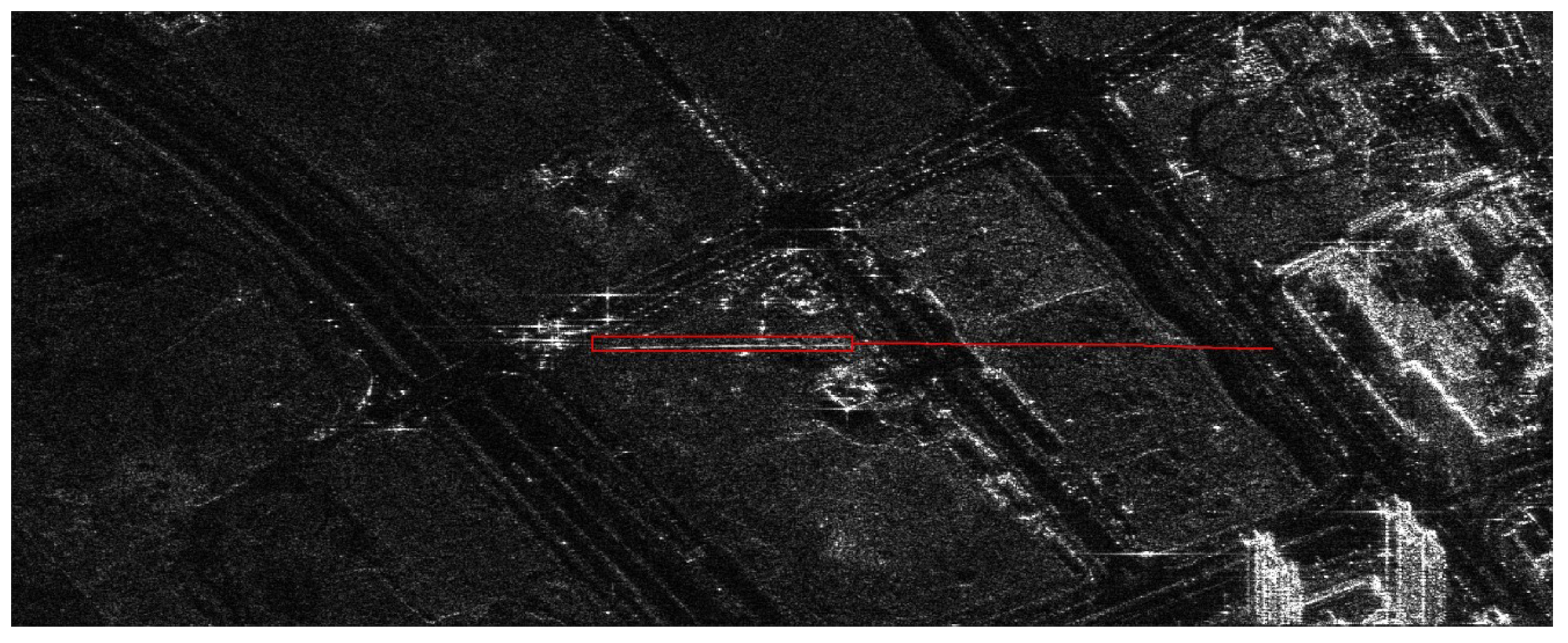
Last, for better illustration, the extracted track information is superimposed on the subaperture image with higher resolution as the final output. We use the final output to make an animation file attached with this paper, and the reader can see the overall tracking result (see Supplementary GIF S1). The example tracking result is illustrated as in Figure 21. The red line denotes the target’s trace, and the red box means its minimal bounding box in the current image. In the figure, the reader can see that the movement is persevered and tracked, and the minimal bounding box matches the area that the target occupied, therefore, the presented modified logarithm background subtraction algorithm is validated.
5.2. Performance Analysis on Background Image Generating and Subtraction
In this section, we make performance analysis on a parameter of the number of images in OSLI (otherwise the aperture length); it is the key parameter in background generation and subtraction step.
The performance is characterized by parameter of SCNR (Signal to Clutter and Noise Ratio, SCNR) improvement . The parameter changes along the number of images in OSLI n. Its formula is given as (22).
The first term in (22) is the target’s SCNR in a foreground image, and the second term is target’s SCNR in original image. and are the maximum intensity of moving target signature and reference clutter respectively. and are the intensity values extracted from the same position as and after subtracting the background generated with a different number of images n.
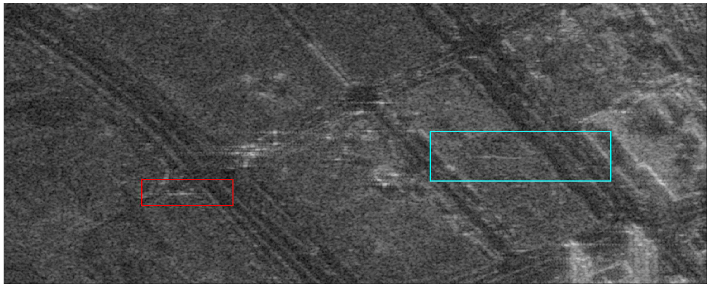
We use the 18th image to perform the analysis as shown in Figure 22. The red box shows a point scatter which is selected as the reference clutter. is extracted from its maximum value. The blue box denotes the moving target area where the is extracted. Then, we apply the background generation and subtraction with different . The examples of background and foreground images of blue box area are shown as Figure 23.
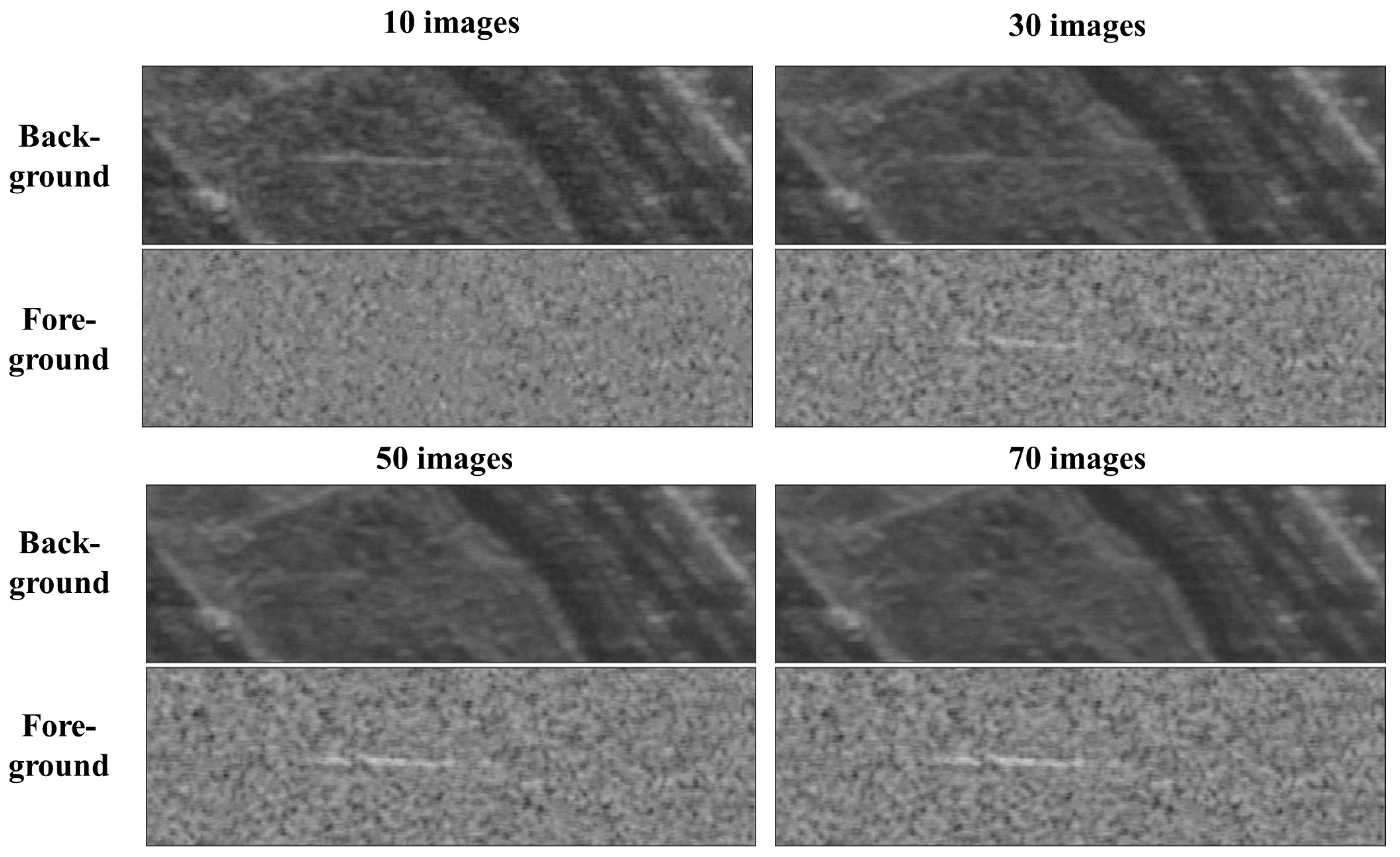
The examples show results using 10, 30, 50, 70 images to perform background generation and subtraction. The first and third rows are the background image. The second and fourth rows are the foreground image. In ten image result, the moving target signature is not filtered, thus, the target signature is canceled in the corresponding foreground. When increasing n, the background image becomes cleaner and the target signature becomes stronger in the foreground image. In 70 image result, the target signature is almost filtered and the target signature is the strongest among the four examples. Thus, it is clear that the more images are used, the better performance we can obtain.
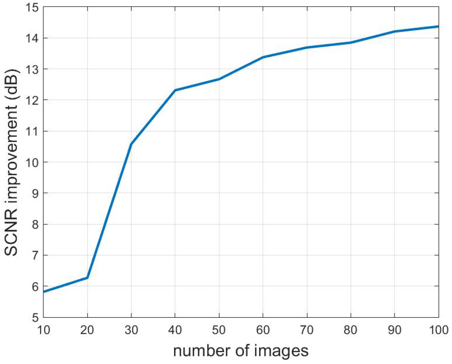
Furthermore, to analyse the performance quantitatively, we apply (22) to the data. The curve of versus number of images n is shown in Figure 24. From figure we can see that along with n, the becomes bigger, which validates the previous analysis. The maximum improvement 14.37 dB is achieved at 100 images, therefore, using 100 images is the optimal parameter for background generation and subtraction in this Gaofen-3 data experiment.
6. Conclusions
In this paper, a new method entitled modified logarithm background subtraction which utilizes the spotlight SAR image to detect ground moving targets is presented. The method is based on logarithm background subtraction (also designed by our team), which is originally developed for airborne SAR. It uses the azimuth subaperture image sequence to model the background (static scene), then detecting moving targets by subtraction process. When applying the original algorithm to the spaceborne spotlight SAR data, a high false alarm problem occurs. To tackle the high false alarm problem due to the target’s low signal-to-noise-ratio (SNR) in the spaceborne case, several improvements are made. First, to preserve most of the moving target signatures, a low threshold CFAR (constant false alarm rate) detector is used to get the coarse detection. Second, because the moving target signatures have higher density than false detections in the coarse detection, a modified DBSCAN (density-based spatial-clustering-of-applications-with-noise) clustering method is then adopted to reduce the false alarm. Third, the Kalman tracker is used to exclude the residual false detections, due to the real moving target signature has dynamic behavior. The proposed method is validated by real data, the shown results also prove the feasibility of the proposed method for both Gaofen-3 and other spaceborne systems.
Although the method is demonstrated with real data, there are also some issues to be solved. First thing is to test the algorithm on more scenes. Second, is to estimate the target’s velocity. From the signal model deduced in this paper, one can find that the range speed can not be calculated via a target’s motion in image space. There are two solutions to this problem. One is to introduce a road model to estimate the velocity. The other one is to combine the multi-channel technique like ATI, since Gaofen-3 is a dual channel configuration. The later one is a more interesting solution. For classical dual channel techniques, they have detection problems like blind speed and not sensitive to target’s azimuth speed. However, the proposed method is sensitive to the azimuth speed and has no blind speed problem. Thus, combining the proposed method and classical dual channel techniques should achieve better performance. The possibility of combining the spotlight mode and dual channel moving target detection mode in Gaofen-3 SAR sensor is now being studied.
Supplementary Materials
The following are available online at https://www.mdpi.com/2072-4292/11/10/1190/s1, GIF S1: supplementary files.zip.
Author Contributions
Under the supervision of Y.L., W.S. performed the experiments and analysis. W.S. wrote the manuscript. B.H. provided the data. W.H. and Y.W. gave valuable advices on manuscript writing.
Funding
This work was supported by the National Natural Science Foundation of China under Grant 61571421 and Grant 61431018.
Conflicts of Interest
The authors declare no conflict of interest.
References
- Dragosevic, M.V.; Burwash, W.; Chiu, S. Detection and Estimation with RADARSAT-2 Moving-Object Detection Experiment Modes. IEEE Trans. Geosci. Remote Sens. 2012, 50, 3527–3543. [Google Scholar] [CrossRef]
- Cerutti-Maori, D.; Sikaneta, I.; Gierull, C.H. Optimum SAR/GMTI Processing and Its Application to the Radar Satellite RADARSAT-2 for Traffic Monitoring. IEEE Trans. Geosci. Remote Sens. 2012, 50, 3868–3881. [Google Scholar] [CrossRef]
- Baumgartner, S.V.; Krieger, G. Dual-Platform Large Along-Track Baseline GMTI. IEEE Trans. Geosci. Remote Sens. 2016, 54, 1554–1574. [Google Scholar] [CrossRef]
- Gierull, C.H. Statistical analysis of multilook SAR interferograms for CFAR detection of ground moving targets. IEEE Trans. Geosci. Remote Sens. 2004, 42, 691–701. [Google Scholar] [CrossRef]
- Lightstone, L.; Faubert, D.; Rempel, G. Multiple phase centre DPCA for airborne radar. In Proceedings of the 1991 IEEE National Radar Conference, Los Angeles, CA, USA, 12–13 March 1991; pp. 36–40. [Google Scholar] [CrossRef]
- Makhoul, E.; Baumgartner, S.V.; Jager, M.; Broquetas, A. Multichannel SAR-GMTI in Maritime Scenarios with F-SAR and TerraSAR-X Sensors. IEEE J. Sel. Top. Appl. Earth Obs. Remote Sens. 2015, 8, 5052–5067. [Google Scholar] [CrossRef]
- Pastina, D.; Turin, F. Exploitation of the COSMO-SkyMed SAR System for GMTI Applications. IEEE J. Sel. Top. Appl. Earth Obs. Remote Sens. 2015, 8, 966–979. [Google Scholar] [CrossRef]
- Ouchi, K. On the multilook images of moving targets by synthetic aperture radars. IEEE Trans. Antennas Propag. 1985, 33, 823–827. [Google Scholar] [CrossRef]
- Kirscht, M. Detection and imaging of arbitrarily moving targets with single-channel SAR. IEE Proc. Radar Sonar Navig. 2003, 150, 7–11. [Google Scholar] [CrossRef]
- Henke, D.; Magnard, C.; Frioud, M.; Small, D.; Meier, E.; Schaepman, M.E. Moving-Target Tracking in Single-Channel Wide-Beam SAR. IEEE Trans. Geosci. Remote Sens. 2012, 50, 4735–4747. [Google Scholar] [CrossRef] [Green Version]
- Shen, W.; Lin, Y.; Yu, L.; Xue, F.; Hong, W. Single Channel Circular SAR Moving Target Detection Based on Logarithm Background Subtraction Algorithm. Remote Sens. 2018, 10, 742. [Google Scholar] [CrossRef]
- Sun, J.; Yu, W.; Deng, Y. The SAR Payload Design and Performance for the GF-3 Mission. Sensors 2017, 17, 2419. [Google Scholar] [CrossRef]
- Han, B.; Ding, C.; Zhong, L.; Liu, J.; Qiu, X.; Hu, Y.; Lei, B. The GF-3 SAR Data Processor. Sensors 2018, 18, 835. [Google Scholar] [CrossRef]
- Jao, J.K. Theory of synthetic aperture radar imaging of a moving target. IEEE Trans. Geosci. Remote Sens. 2001, 39, 1984–1992. [Google Scholar] [CrossRef] [Green Version]
- Chapman, R.D.; Hawes, C.M.; Nord, M.E. Target Motion Ambiguities in Single-Aperture Synthetic Aperture Radar. IEEE Trans. Aerosp. Electron. Syst. 2010, 46, 459–468. [Google Scholar] [CrossRef]
- Shen, W.; Lin, Y.; Chen, S.; Xue, F.; Yang, Y.; Hong, W. Apparent Trace Analysis of Moving Target with Linear Motion in Circular SAR Imagery. In Proceedings of the EUSAR 2018 12th European Conference on Synthetic Aperture Radar, Aachen, Germany, 4–7 June 2018; pp. 1–4. [Google Scholar]
- Raney, R.K. Synthetic Aperture Imaging Radar and Moving Targets. IEEE Trans. Aerosp. Electron. Syst. 1971, AES-7, 499–505. [Google Scholar] [CrossRef]
- Huynh-The, T.; Banos, O.; Lee, S.; Kang, B.H.; Kim, E.; Le-Tien, T. NIC: A Robust Background Extraction Algorithm for Foreground Detection in Dynamic Scenes. IEEE Trans. Circuits Syst. Video Technol. 2017, 27, 1478–1490. [Google Scholar] [CrossRef]
- Huynh-The, T.; Hua, C.; Tu, N.A.; Kim, D. Locally Statistical Dual-Mode Background Subtraction Approach. IEEE Access 2019, 7, 9769–9782. [Google Scholar] [CrossRef]
- Wu, Q.Z.; Jeng, B.S. Background subtraction based on logarithmic intensities. Pattern Recognit. Lett. 2002, 23, 1529–1536. [Google Scholar] [CrossRef]
- Moser, G.; Serpico, S.B. Generalized minimum-error thresholding for unsupervised change detection from SAR amplitude imagery. IEEE Trans. Geosci. Remote Sens. 2006, 44, 2972–2982. [Google Scholar] [CrossRef] [Green Version]
- Radke, R.J.; Andra, S.; Al-Kofahi, O.; Roysam, B. Image change detection algorithms: A systematic survey. IEEE Trans. Image Process. 2005, 14, 294–307. [Google Scholar] [CrossRef] [PubMed]
- Zhao, Y.; Lin, Y.; Hong, W.; Yu, L. Adaptive imaging of anisotropic target based on circular-SAR. Electron. Lett. 2016, 52, 1406–1408. [Google Scholar] [CrossRef]
- Gao, G.; Wang, X.; Niu, M.; Zhou, S. Modified log-ratio operator for change detection of synthetic aperture radar targets in forest concealment. J. Appl. Remote Sens. 2014, 8, 8–10. [Google Scholar] [CrossRef]
- Novak, L.M.; Owirka, G.J.; Netishen, C.M. Performance of a High-Resolution Polarimetric SAR Automatic Target Recognition System. Linc. Lab. J. 1993, 6, 1. [Google Scholar]
- Ester, M.; Kriegel, H.P.; Sander, J.; Xu, X. A Density-based Algorithm for Discovering Clusters a Density-based Algorithm for Discovering Clusters in Large Spatial Databases with Noise. In Proceedings of the Second International Conference on Knowledge Discovery and Data Mining, Portland, OR, USA, 2–4 August 1996; pp. 226–231. [Google Scholar]
- Selim, S.Z.; Ismail, M.A. K-Means-Type Algorithms: A Generalized Convergence Theorem and Characterization of Local Optimality. IEEE Trans. Pattern Anal. Mach. Intell. 1984, PAMI-6, 81–87. [Google Scholar] [CrossRef]
- Kovvali, N.; Banavar, M.; Spanias, A. An Introduction to Kalman Filtering with MATLAB Examples; Morgan & Claypool: San Rafael, CA, USA, 2013. [Google Scholar]
Figure 1.
The upper SAR image shows the selected scene for test. The moving target signature is bounded by the blue box. To show the motion of moving target’s signature, four subaperture images of the area bounded by the blue box are generated as shown in bottom. From image 1 to 4, it is clear that the target signature moves from right to the left.

Figure 2.
Acquisition geometry.

Figure 3.
The azimuth and range speed which can induce indistinguishable cases using parameter of Gaofen-3.
Figure 3.
The azimuth and range speed which can induce indistinguishable cases using parameter of Gaofen-3.

Figure 4.
Subfigure (a–c) are the images of target A,B,C in Table 3 respectively. The blue ‘*’ denotes the calculated image position.
Figure 4.
Subfigure (a–c) are the images of target A,B,C in Table 3 respectively. The blue ‘*’ denotes the calculated image position.

Figure 5.
The target’s azimuth smearing length in 12.5 s (Gaofen-3 illuminating time in staring spotlight mode) versus azimuth speed.
Figure 5.
The target’s azimuth smearing length in 12.5 s (Gaofen-3 illuminating time in staring spotlight mode) versus azimuth speed.

Figure 6.
The flow chart of proposed method.

Figure 7.
The illustration of subaperture processing.

Figure 8.
The illustration of intensity normalization.

Figure 9.
The illustration of CFAR detector.

Figure 10.
The (a,b) are illustration of conventional and modified DBSCAN method respectively.

Figure 11.
The processing example using 18th image of the OSLI sequence. Subfigure (a) is the 18th image. Subfigure (b) is the corresponding background image generated with OSLI (100 images). Subfigure (c) is the foreground image obtained by using (a) minus (b). Blue box denotes the target signature’s position.

Figure 12.
The histograms of 18th and 68th image before and after applying intensity normalization.

Figure 13.
The histograms of foreground image.

Figure 14.
The CFAR detection result of 18th image. The blue box denotes the moving target.

Figure 15.
Subfigure (a,b) are the result of applying the conventional DBSCAN and modified DBSCAN method to 18th image respectively. Each cluster is bounded with the red rectangle according to minimal bounding box parameter. The blue arrow points to the moving target.
Figure 15.
Subfigure (a,b) are the result of applying the conventional DBSCAN and modified DBSCAN method to 18th image respectively. Each cluster is bounded with the red rectangle according to minimal bounding box parameter. The blue arrow points to the moving target.

Figure 16.
Clustering accuracy of real target signature with different and . Black part denotes the real target signatures are classified as different clusters (kind (b)). The orange part denotes the real and false target signatures are classified as one cluster (kind (c)). The white part means real target signatures are classified as one cluster (kind (a)).

Figure 17.
False alarm rate versus when . The curve is divided into three parts according to the clustering accuracy results kind (a), kind (b) and kind (c).
Figure 17.
False alarm rate versus when . The curve is divided into three parts according to the clustering accuracy results kind (a), kind (b) and kind (c).

Figure 18.
Tracking results of first image and 18th image. Blue arrow denotes the moving target. (a) is the first image, all ten clusters are used to initialize the tracks. The clusters correspond to the tracks and are labeled with red rectangles. (b) is the result of 18th image, the red line denotes the moving trace. It is clear that there are only two tracks which are updating after 18 iterations.

Figure 19.
The overall tracked iterations and missing iterations of ten tracks in all 100 iterations. The blue denotes the tracked iterations and orange denotes the missing iterations. The 5th track is real moving target, which shows it is tracked in 100 iterations without missing. The rest tracks correspond to the false detections stop updating after 20 iterations.

Figure 20.
The curve of total tracked iterations of ten clusters versus different . Target 5 is the real moving target, the rest is the false detections.
Figure 20.
The curve of total tracked iterations of ten clusters versus different . Target 5 is the real moving target, the rest is the false detections.

Figure 21.
The final tracking result which is generated by superimposing track’s information on higher resolution subaperture images. The red line denotes the target’s trace, and the red box means its minimal bounding box in the current image.
Figure 21.
The final tracking result which is generated by superimposing track’s information on higher resolution subaperture images. The red line denotes the target’s trace, and the red box means its minimal bounding box in the current image.

Figure 22.
The 18th subaperture image in 100 image sequence. The reference clutter is denoted with a red box, and the blue box denotes a moving target signature.
Figure 22.
The 18th subaperture image in 100 image sequence. The reference clutter is denoted with a red box, and the blue box denotes a moving target signature.

Figure 23.
The examples of background and foreground image of blue box area in Figure 22. The example shows results using 10, 30, 50, 70 images to perform background generation and subtraction.
Figure 23.
The examples of background and foreground image of blue box area in Figure 22. The example shows results using 10, 30, 50, 70 images to perform background generation and subtraction.

Figure 24.
The curve of versus number of images n.


Table 1.
Dataset Parameters.
| Symbol | Parameter | Value | Symbol | Parameter | Value |
|---|---|---|---|---|---|
| Wavelength | 0.056 m | Range To Scene Center | km | ||
| Platform Velocity | 7568 m/s | Azimuth Observing Time | s | ||
| Look Angle | Aperture Width | ~ | |||
| Bandwidth | 240 MHz | Range Spacing | m | ||
| PRF | 3742.7 Hz | Azimuth Spacing | m |
Table 2.
Target/SAR motion functions.
| Directions | SAR | Target |
|---|---|---|
| Azimuth | ||
| Range | 0 | |
| Height | 0 |
Table 3.
Target motion parameters.
| Parameter | Target A | Target B | Target C |
|---|---|---|---|
| 5 m/s | 0 m/s | 5 m/s | |
| 0 m/s | 5 m/s | 5 m/s | |
| 934.6 km | 934.6 km | 934.6 km |
Table 4.
Maximal Azimuth Moving Distance and Corresponding Azimuth Speed.
| Track Number | 1 | 2 | 3 | 4 | 5 | 6 | 7 | 8 | 9 | 10 |
|---|---|---|---|---|---|---|---|---|---|---|
| distance (m) | 12.8 | 35.6 | 37.4 | 36.6 | 417.8 | 11.2 | 21.9 | 22.1 | 27.6 | 31.6 |
| speed (m/s) | 0.5 | 1.4 | 1.5 | 1.5 | 16.7 | 0.4 | 0.9 | 0.9 | 1.1 | 1.3 |
© 2019 by the authors. Licensee MDPI, Basel, Switzerland. This article is an open access article distributed under the terms and conditions of the Creative Commons Attribution (CC BY) license (http://creativecommons.org/licenses/by/4.0/).
Share and Cite
MDPI and ACS Style
Shen, W.; Hong, W.; Han, B.; Wang, Y.; Lin, Y. Moving Target Detection with Modified Logarithm Background Subtraction and Its Application to the GF-3 Spotlight Mode. Remote Sens. 2019, 11, 1190. https://doi.org/10.3390/rs11101190
AMA Style
Shen W, Hong W, Han B, Wang Y, Lin Y. Moving Target Detection with Modified Logarithm Background Subtraction and Its Application to the GF-3 Spotlight Mode. Remote Sensing. 2019; 11(10):1190. https://doi.org/10.3390/rs11101190
Chicago/Turabian StyleShen, Wenjie, Wen Hong, Bing Han, Yanping Wang, and Yun Lin. 2019. "Moving Target Detection with Modified Logarithm Background Subtraction and Its Application to the GF-3 Spotlight Mode" Remote Sensing 11, no. 10: 1190. https://doi.org/10.3390/rs11101190
Note that from the first issue of 2016, this journal uses article numbers instead of page numbers. See further details here.