Hyperspectral and Multispectral Image Fusion Using Cluster-Based Multi-Branch BP Neural Networks


1
Institute for Artificial Intelligence, Beijing National Research Center for Information Science and Technology, State Key Laboratory of Intelligent Technology and Systems, Department of Electronic Engineering, Tsinghua University, Beijing 100084, China
2
Faculty of Information Technology, Beijing Univ. of Technology, Beijing 100124, China
3
School of Opte-Electronics, Beijing Institute of Technology, Beijing 100081, China
*
Author to whom correspondence should be addressed.
Remote Sens. 2019, 11(10), 1173; https://doi.org/10.3390/rs11101173
Submission received: 22 April 2019
/
Revised: 11 May 2019
/
Accepted: 13 May 2019
/
Published: 16 May 2019
(This article belongs to the Special Issue Quality Improvement of Remote Sensing Images)
Abstract
:Fusion of the high-spatial-resolution hyperspectral (HHS) image using low-spatial- resolution hyperspectral (LHS) and high-spatial-resolution multispectral (HMS) image is usually formulated as a spatial super-resolution problem of LHS image with the help of an HMS image, and that may result in the loss of detailed structural information. Facing the above problem, the fusion of HMS with LHS image is formulated as a nonlinear spectral mapping from an HMS to HHS image with the help of an LHS image, and a novel cluster-based fusion method using multi-branch BP neural networks (named CF-BPNNs) is proposed, to ensure a more reasonable spectral mapping for each cluster. In the training stage, considering the intrinsic characteristics that the spectra are more similar within each cluster than that between clusters and so do the corresponding spectral mapping, an unsupervised clustering is used to divide the spectra of the down-sampled HMS image (marked as LMS) into several clusters according to spectral correlation. Then, the spectrum-pairs from the clustered LMS image and the corresponding LHS image are used to train multi-branch BP neural networks (BPNNs), to establish the nonlinear spectral mapping for each cluster. In the fusion stage, a supervised clustering is used to group the spectra of HMS image into the clusters determined during the training stage, and the final HHS image is reconstructed from the clustered HMS image using the trained multi-branch BPNNs accordingly. Comparison results with the related state-of-the-art methods demonstrate that our proposed method achieves a better fusion quality both in spatial and spectral domains.

1. Introduction
Hyperspectral (HS) images can provide abundant spectral and spatial information simultaneously, and have been widely used in various fields. However, the increasing of spectral bands in the HS imaging process results in the limitation on the spatial resolution [1]. On the other hand, multispectral (MS) images, which only have a few spectral bands, generally have much higher spatial resolution, when compared to HS images. Thus, a more useful high-spatial-resolution hyperspectral (HHS) image can be obtained, if we can fuse a low-spatial-resolution hyperspectral (LHS) image with a high-spatial-resolution multispectral (HMS) image over the same scene.
A number of methods have been proposed for HS and MS image fusion, which can be mainly divided into four groups: Pansharpening based, Bayesian based, dictionary learning based and neural network based methods. Specifically, pansharpening-based methods have been proposed to fuse a high-spatial-resolution panchromatic image with a low-spatial-resolution multispectral (LMS) image [2,3] or an LHS image [4]. Using maximum a posteriori (MAP) estimation, Hardie et al. [5] proposed an enhancement method for hyperspectral image using a panchromatic image. In extension, Paris et al. [6] proposed a method to enhance the spatial resolution of MS multiresolution images that have more than one high-spatial-resolution channel. Using WorldView-3 data, Selva et al. [7] proposed an extended pansharpening method to improve the spatial resolution of hyperspectral image, which introduces the histogram matching operation into the synthesized band variant. An extension of the pansharpening based method has been proposed by Zhu et al. [8], which simplifies the LHS and HMS image fusion as several pansharpening processes. It can be seen as a spatial super-resolution process of the LHS image in each band. As for spatial super-resolution, using single image super-resolution and hybrid color mapping (HCM), Hardie et al. [9] proposed an LHS and color image fusion method, where the HCM is defined as a linear transformation solved by least square solution.
To further improve fusion quality, both in spatial and spectral domains, Bayesian-based methods have been proposed, which use Gaussian distribution priors to build various estimators. Based on Bayesian inference, an LHS and HMS image fusion method was proposed by Wei et al. [10]. Besides, a fast fusion method has also been proposed by solving a Sylvester equation associated with a Bayesian estimator [11].
Recently, dictionary learning based methods have also been widely used in hyperspectral image fusion. Huang et al. [12] proposed an LHS and HMS image fusion method, where pure spectral signatures are conducted by a trained spectral dictionary. A coupled matrix factorization method was proposed by Yokoya et al. [13], which unmixed both hyperspectral and multispectral images into abundances and endmembers, i.e., a special form of spectral dictionary. Besides, Simoes et al. [14] proposed an LHS and HMS image fusion method using total variation regularization, in which the spectral dictionary consists of the pure spectral signatures of endmembers. Han et al. [15] proposed a fusion method using sparse representation, where the spectral dictionary consists of the mixed spectral signatures. Moreover, Akhtar et al. [1] offered a sparse representation approach with non-negative constraint using a learned spectral dictionary, which assumes that similar pixels have the same abundances in the estimation of sparse coefficients. Using spectral and spatial dictionaries simultaneously, Nezhad et al. [16] proposed a spectral unmixing and sparse coding based method for the spatial resolution improvement of hyperspectral images.
Very recently, neural network based methods have been widely used in many different areas with much more better performance, such as super-resolution [17], target detection [18], and have also been used in image fusion tasks. Using deep CNN with two branches, Yang et al. [19] proposed a fusion method to extract features from LHS and HMS images, respectively. Palsson et al. [20] firstly proposed a 3-D convolutional neural network (3D-CNN) method to fuse LHS and HMS image into a HHS image. Assuming that the decimation filter between MS and HS image is the same at different spatial resolution scales, an HHS image can be obtained, using the decimation filter estimated with a 3D-CNN, which uses the spatially decimated LMS and LHS image patch-pairs as learning basis. In this case, as the spectral information has not been changed, it can be seen as a spatial super-resolution of the LHS image, while some detailed structural information may be lost, if the decimation filter has not been estimated perfectly.
Considering that HMS and LHS image fusion is usually formulated as a spatial super-resolution of the LHS image, and may result in the loss of spatial information, we formulate it in a new way of spectral super-resolution of the HMS image. Furthermore, a cluster-based multi-branch BPNNs structure (named as CF-BPNNs) is proposed, to ensure a more reasonable spectral mapping for each cluster. In the training stage, owing to the intrinsic characteristic that the spectra are more similar within each cluster than that between clusters and as are the corresponding spectral mapping, unsupervised clustering is used to divide the spectra of the LMS image into several clusters according to spectral correlation. Then, the spectrum-pairs from the clustered LMS image and the corresponding LHS image are used to train the multi-branch BPNNs, to establish the spectral mapping for each cluster. In the fusion stage, since the spectral mapping established in the low-scale spatial resolution can still hold in high-scale spatial resolution, a supervised clustering is used to obtain the corresponding clustered spectra of the HMS image, and the final HHS image is reconstructed from the clustered HMS image using the trained multi-branch BPNNs, accordingly.
The main contributions of this paper are as follows.
- The fusion problem of HMS and LHS image is firstly formulated as a nonlinear spectral mapping from an HMS to HHS image with the help of an LHS image.
- A cluster-based learning method using multi-branch BPNNs is proposed, to ensure a more reasonable spectral mapping for each cluster.
- An associative spectral clustering method is proposed to ensure that the clusters used in the training and fusion stage are consistent.
2. Problem Formulation
An HHS image can be generated by using an HMS image and an LHS image over the same scene, where and () represent the number of pixels per band in and , and () represent the number of spectral bands in and , respectively. As a degraded version of the HHS image in spectral and spatial domain, the relationships between the observed image , and the target HHS image can be formulated as:
where, denotes the spectral response function in the spectral domain, denotes the blurring and down sampling operator in the spatial domain, when denotes the down sampling rate in both vertical and horizontal directions. and denote the zero-mean Gaussian noise in the observation model, which is a popular assumption in the imaging process modeling [10,20]. With a spatial degraded of , the LMS image can be expressed as:
Substituting Equation (2) into Equation (3) leads to the following equation:
where, denotes the zero-mean Gaussian noise. As can be seen in Equation (4), it is a spatial degradation of Equation (1), while the spectral response function has not been changed. In other words, the inverse matrix of the spectral response function , i.e., the spectral mapping established from to in the low-scale spatial resolution, is identical to that in the high-scale spatial resolution (the spectral mapping from to ). Since the target HHS image in Equation (1) is not available, the spectral mapping from to can be learned from to equivalently.
Solving from in Equation (4) is an underdetermined inverse problem with infinite solutions. However, the solution of Equation (4) may become unique when it is solved in a suitable subspace. Considering that the spectral mapping is increasingly easier to estimate, when the spectrum-pairs from and the corresponding become more similar, a suitable subspace can be formed by clustering similar spectra in the following ways:
where and denote the clustered subspace in cluster , and is the total number of clusters. As can be seen in Equation (5), the spectral mapping from to for each cluster can be learned using the spectrum-pairs formed by the clustered spectra of and the corresponding spectra of . It is worth mentioning that the purpose of spectra clustering in Equation (5) is to cluster similar spectra into several subspaces, instead of making an accurate classification for the ground surface objects. Besides, Figure 1 shows the spectral mappings of different clusters using typical spectrum-pairs of and on the AVIRIS dataset, which will be described in more detail in Section 4. As can be seen in Figure 1, the spectral mappings are similar within each cluster, while they are different among different clusters. In other words, the spectral mapping learned in each subspace according to Equation (5) is more reasonable than that learned in the whole spectrum space.
If the spectra in can be clustered into the same subspace as Equation (5), Equation (1) can be rewritten as:
where and denote the corresponding clustered subspace in cluster , and . As the spectral mapping established in the low-scale spatial resolution is identical to that in the high-scale spatial resolution, the target HHS image can be obtained from the clustered HMS image according to Equation (6), by using the trained nonlinear spectral mapping of its corresponding cluster in Equation (5).
3. Proposed Method
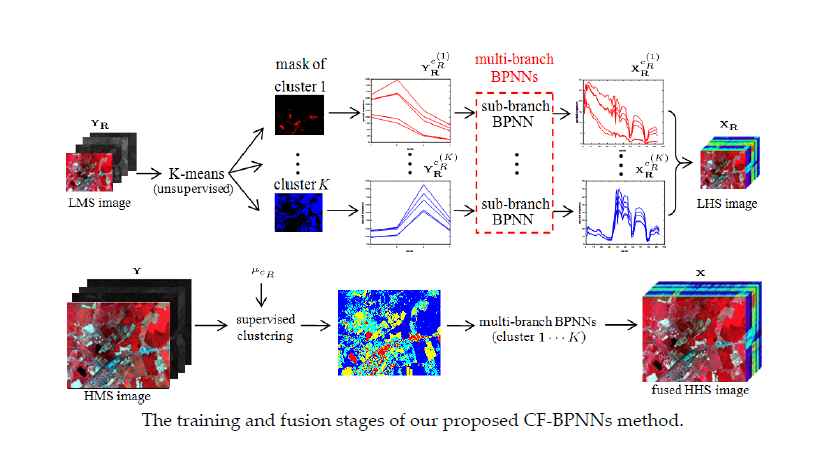
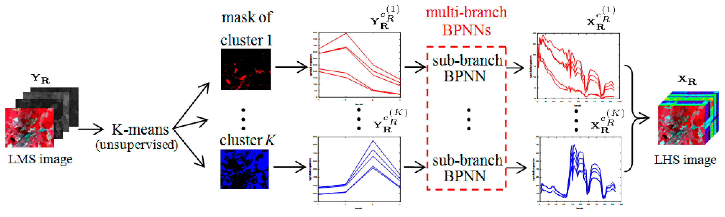
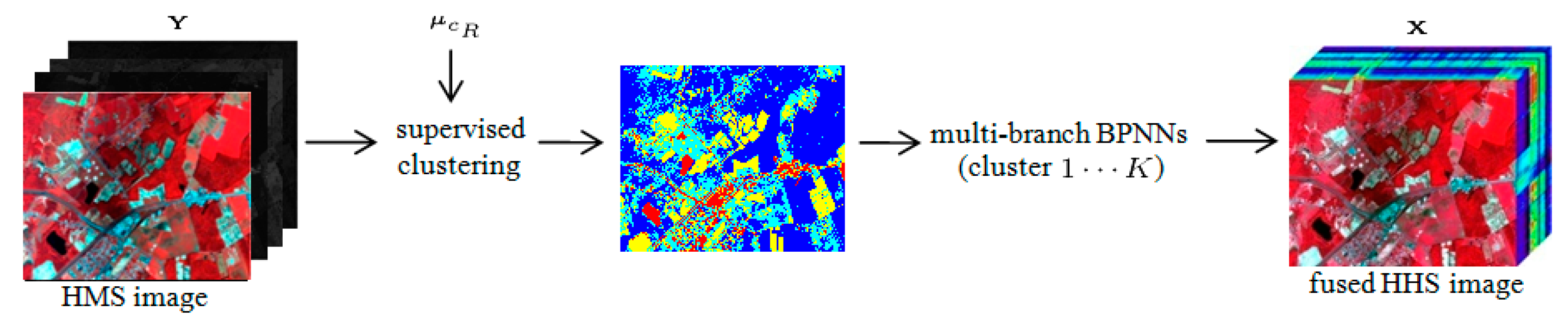
The frameworks of the two stages of our proposed CF-BPNNs method are shown in Figure 2 and Figure 3, respectively. In the training stage shown in Figure 2, an unsupervised spectral clustering is performed on the spectra of the LMS image. Then, the clustered spectra of the LMS image and those of its corresponding LHS image together form spectrum-pairs. Using clustered spectrum-pairs as a learning basis, a series of sub-branch BPNNs is constructed to establish the nonlinear spectral mapping from LMS to LHS image for each cluster. In the fusion stage shown in Figure 3, after an associative spectral clustering on the HMS image, each spectrum in the target HHS image is reconstructed by using the trained nonlinear spectral mapping of its corresponding cluster. The overall framework of our proposed method is shown in Figure 4. As can be seen in Figure 4, the spatial information is provided directly by the HMS image, and the spectral information is provided by the LHS and LMS image through spectral mapping, which is represented by multi-branch BPNNs. The details of our proposed method are described as follows:
3.1. Associative Spectral Clustering for LMS and HMS Images
In the training stage, the spectra of LMS image are grouped into clusters using the minimum intra-cluster distance criterion. It can be described as:
where denotes the th column of , denotes the clustering center of subspace , and denotes the distance between two spectra. Here, spectral angle is employed as the measure of distance:
Given the number of clusters , the above subspace division problem can be viewed as an unsupervised clustering problem that can be solved by the k-means algorithm [21], and the cluster centers can be initialized by the k-means++ algorithm [22], as the k-means++ algorithm consistently outperformed k-means algorithm in both speed and clustering accuracy. Additionally, the corresponding clustered spectra of the LHS image are obtained using the “mask” determined during the above unsupervised clustering, as LMS image is the spectral degraded version of the LHS image with an absolute one-to-one correspondence in the spatial domain.
In the fusion stage, since the spectral mapping established in the low-scale spatial resolution is identical to that in the high-scale spatial resolution, for each cluster, the spectral mapping learned by using the LMS and LHS spectrum-pairs can also be used to the HMS and HHS image. But, the key here is that the spectra in the HMS image should be clustered exactly into the corresponding subspaces determined by the spectra of the LMS image during the training stage. Thus, each spectrum of the HMS image should be supervised clustered into clusters using the above determined clustering center of the LMS image , by the following optimization problem:
The above unsupervised clustering for the LMS image and supervised clustering for the HMS image can be seen as an associative spectral clustering method, carried out before the spectral mapping.
3.2. Multi-Branch BPNNs and Spectral Mapping
To solve the challenging underdetermined inverse problem in Equation (5), we construct a multi-branch BPNNs for different clusters. Specifically, we treat the spectral mapping in each cluster as a nonlinear spectral mapping to be represented by one sub-branch BPNN, since BPNN has a strong nonlinear mapping capability even with a few hidden layers. A basic three-layer BPNN shown in Figure 5, including one hidden layer, is used here for each sub-branch. The output of the BPNN is:
where and denote the inputs and outputs, respectively, denotes the nonlinear active function in the hidden layer, denotes the linear active function in the output layer, () are the weights and offsets, respectively.
In the training stage, in each sub-branch BPNN, the input is the spectrum from LMS image of one cluster, and the output is the corresponding spectrum from LHS image. As shown in Figure 5, the number of atoms in and is equal to and , i.e., the number of spectral bands in and , respectively. After training, the multi-branch BPNNs established a series of nonlinear spectral mapping between LMS and LHS image for different clusters.
In the fusion stage, according to the intrinsic characteristic described above, i.e., spectral mapping established in the low-scale spatial resolution can also hold in the high-scale spatial resolution, the target HHS image can be obtained from the clustered HMS image, using the trained multi-branch BPNNs directly, as shown in Figure 3. For each sub-branch BPNN, the input is the spectrum from the corresponding clustered HMS image, and the output is the reconstructed spectrum in the target HHS image.
4. Experimental Results and Discussion
4.1. Comparison Methods and Quality Metrics
To evaluate the fusion performance of our proposed CF-BPNNs method, the related state-of-the-art methods for LHS and HMS image fusion, such as coupled nonnegative matrix factorization (CNMF) method [13], the generalization of simultaneous orthogonal matching pursuit (G-SOMP+) method [1], the hyperspectral super-resolution (Hysure) method [14], the fast fusion based on sylvester equation (FUSE) method [11], the collaborative representation using local adaptive dictionary pair (LACRF) method [8], the non-factorization sparse representation and error matrix estimation (NFSREE) method [15] and the most new 3D-CNN method [20] are used as comparisons. Furthermore, six full-reference quality metrics are used to evaluate fusion performances, including mean square error (MSE), peak-signal-to-noise ratio (PSNR) [23], spectral angle mapper (SAM) [10], universal image quality index (UIQI) [10], relative dimensionless global error in synthesis (ERGAS) [24], and structural similarity (SSIM) [23]. All of the above methods are conducted using MATLAB R2015b on a computer with a 3.60 GHz CPU and 28 GB RAM.
4.2. Comparison on the First Dataset
In this part of the experiment, the original HS image was acquired on 5 July 1996 by the AVIRIS airborne system [25], ranging from 400 nm to 2500 nm, with a dimension of 512 × 614 × 193. The upper left corner of the original HS image with a dimension of 500 × 600 × 93 is used as the ground-truth of the HHS image, to make its size an integer multiple of the down sampling rate; some of the original bands 1–2, 105–115, 150–170, 223–224 have been removed, considering the serious effects of water absorption. Spectral response functions used in this experiment are the IKONOS-like spectral response functions [10], with a dimension of 4 × 93, covering visible and near infrared bands (). Consequently, the HMS image can be simulated following Equation (1) with a dimension of 500 × 600 × 4, shown as the false color image in Figure 6b. As shown in Figure 6a, the LHS image with a dimension of 100 × 120 × 93 is simulated by a 5 × 5 Gaussian kernel with the standard deviation , and the down sampling rate in both vertical and horizontal directions, which takes one of every five elements in the spatial domain. When the down sampling rate is set to 5, 3.0 is a reasonable value for the standard deviation, which ensures a sufficient amount of information delivered from the scene to the acquired image [26]. In the training stage, as an LMS image is obtained using the same blurring and down sampling operator with a dimension of 100 × 120 × 4, the total number of training data is 12,000 spectra. In the associative spectral clustering, the spectra in this LMS image are divided into 10 clusters to balance the spectrum similarity and the number of training data, which means that the number of training data for each cluster roughly becomes 1200 spectra. Particularly in this experiment, the three-layer BPNN used for each sub-branch is a 4-5-93 BPNN, and the number of undetermined parameters in each BPNN is 583. Thus, we can see that the number of training data for each cluster is nearly two times than the number of undetermined parameters, which is sufficient for the training of this BPNN. In each sub-branch BPNN, the maximum training epochs is set to 100, and 15% of the training data is used as the validation data to mitigate overfitting. Besides, the loss function in the training stage is the mean squared error between the target spectra and the mapped spectra; the sigmoid function is used as the active function in the hidden layer, and linear function is used in the output layer.
Table 1 shows the fusion results on AVIRIS dataset using the averaged MSE, PSNR, UIQI, SAM, ERGAS and SSIM metrics. It can be seen that our proposed CF-BPNNs method shows better fusion results, both in spatial and spectral domains, than all the other methods. Particularly, PSNR is improved in 2 dB than that of the other methods, which shows an outperformance in spatial preservation. Moreover, our proposed CF-BPNNs method improves the performance of spectral reconstruction more than 0.17 in SAM, which is significant for the HHS image. Besides, the fusion results in spectral domain on typical pixels are shown in Figure 7. The results also indicate the outperformance of our proposed CF-BPNNs method in spectrum reconstruction.
Figure 8 shows the fusion results of different methods in band 30 with one region zoomed. To get a better visualization, the brightness of all the fusion images has been increased to the same extent. As can be seen in the zoomed region in Figure 8, our proposed CF-BPNNs method performs better than CNMF, G-SOMP+ and NSFREE methods in spatial structure reconstruction. To easily discern the differences between different methods visually, Figure 9 shows the errors of the fused HHS image in MSE and SAM, respectively. The MSE images visualize the magnitude of the error at each pixel in band 30. The SAM images visualize the spatial distribution of spectral angle errors. Compared with other related methods, our proposed method shows an obvious improvement both in MSE and SAM, as shown in Figure 9f, which means a much better performance in spatial and spectral preservation.
4.3. Comparison on the Second Dataset
In this part of the experiment, 3D-CNN method [20] is used as a new additional comparison technique, since it is the first fusion method based on neural networks. However, as the same network structure and parameter adjustments cannot be achieved exactly, the results of 3D-CNN method can only be taken from their original paper, and the comparisons will use the same dataset and the same quality metrics as given in [20]. In this case, the ROSIS Pavia center dataset [27] with a dimension of 512 × 480 × 102, is used as the ground truth of the HHS image. HMS image is simulated with the IKONOS-like spectral response functions mentioned above, with a dimension of 512 × 480 × 4. Besides, three different types of decimation filters, i.e., bicubic, bilinear, and nearest neighbor, are used for LHS images simulation, with dimensions of 128 × 120 × 102. LMS images are simulated using the corresponding decimation filters, with dimensions of 128 × 120 × 4. In this experiment, the number of training data in our proposed method is 128 × 120 spectra.
Table 2 shows the fusion results on the ROSIS Pavia center dataset using averaged ERGAS, SAM and SSIM metrics. The short lines indicate that there is no relevant information available from the original papers, and the best results are in bold; the second best are underlined. As can be seen in Table 2, except the case of the bicubic decimation filter, our proposed method performs best in all the other circumstances. Our proposed method performs best in SSIM, which shows a better spatial structure preservation ability than the 3D-CNN method in all circumstances, and this result is consistent with the problem setting and inference given in Section 1. Besides, since the spectral mapping may cause some spectral distortion, in the case of the bicubic decimation filter, our proposed method shows a little worse but comparable performance in SAM. As multi-branch BPNNs ensures a more reasonable spectral mapping for each cluster, our proposed CF-BPNNs method performs better in SAM than the 3D-CNN method in most circumstances. The fusion results also show the robustness of our proposed method in terms of different decimation filters.
4.4. Discussions on Parameters Selection
To evaluate the effects of key parameters on the performance of our proposed CF-BPNNs method, significant parameters, such as the number of clusters , the signal-to-noise ratio (SNR) for Gaussian noise, and the lengths of filter, are varied on the AVIRIS dataset.
Figure 10a,b plot the PSNR and SAM curves of the fused HHS image, respectively, as a function of the number of clusters . It can be seen that our proposed CF-BPNNs method shows a better performance in spectral reconstruction with much clusters. However, the spatial performance is better when is between 5 and 20. This may be due to the fact that with more clusters, the reduction of training data in each cluster may affect the training performance of sub-branch BPNN, and will further affect the quality of the fused HHS image. Since training time is the major cost of our proposed method, the relationship between the number of clusters and the training time is evaluated and shown in Figure 10c, and it turns out that the maximum training time for each cluster is decreasing with the increasing of , when the total number of training spectrum-pairs is fixed. Figure 10d shows the fusion performance with different SNRs in terms of PSNR. The result shows that the performance of our proposed CF-BPNNs method shows a stable fusion ability, when SNR is higher than 25 dB.
Figure 11a–c plot the PSNR, SAM and SSIM curves of the fused HHS image, respectively, as a function of the lengths of filter. As can be seen in Figure 11, although the PSNR and SAM curves show a slightly downward and upward trend to some extent, the SSIM curve shows a very stable performance against different lengths of the filter. The above experimental results show that our proposed method performs stably with different lengths of the filter, as the variation of each metric is limited to a fairly small range.
4.5. Comparison with and without Clustering
To evaluate the advantages of clustering, in this part of experiment, our proposed CF-BPNNs method is compared with a fusion method without clustering on the AVIRIS dataset mentioned in Section 4.2. Without clustering means that the spectral mapping in Figure 2 is established only using one branch BPNN. The fusion results are shown in Table 3, where the fusion method without clustering is shown as the results of “F-BPNN”.
As can be seen in Table 3, our proposed CF-BPNNs method with clustering shows much better fusion performances than the F-BPNN method without clustering, both in spatial and spectral domains. Specifically, the CF-BPNNs method improves the performance of the fused HHS image over 3 dB in PSNR, and over 0.4 in SAM than the F-BPNN method. That is to say, the fusion method with clustering yields significant performances than that of the method without clustering, both in spatial and spectral preservation.
5. Conclusions
In this paper, we proposed a new LHS and HMS image fusion method using cluster-based multi-branch BPNNs. Specifically, the LHS and HMS image fusion is formulated as a spectral super-resolution problem from an HMS to HHS image with the help of an LHS image. Multi-branch BPNNs are trained using the spectrum-pairs from the clustered LMS and LHS image, to establish the nonlinear spectral mappings for different clusters. Associative spectral clustering is used to ensure that the clusters in the training and fusion stage are consistent. The target HHS image is obtained from the clustered HMS image using the trained multi-branch BPNNs accordingly, as the spectral mapping is the same in different spatial resolution scales. Experimental results on different datasets demonstrated that our proposed CF-BPNNs method performed better, both in spatial and spectral domains than the other related fusion methods.
Funding
This research was funded in part by the National Nature Science Foundation, Grant Number 61501008, and Beijing Natural Science Foundation of China, Grant Number 4172002.
Conflicts of Interest
The authors declare no conflict of interest.
References
- Akhtar, N.; Shafait, F.; Mian, A. Sparse Spatio-Spectral Representation for Hyperspectral Image Super-Resolution; European Conference on Computer Vision; Springer: Berlin/Heidelberg, Germany, 2014; pp. 63–78. [Google Scholar]
- Carper, W.J.; Lillesand, T.M.; Kiefer, R.W. The use of intensity-hue-saturation transformations for merging SPOT panchromatic and multispectral image data. Photogramm. Eng. Remote Sens. 1990, 56, 457–467. [Google Scholar]
- Jiang, C.; Zhang, H.; Shen, H.; Zhang, L. A practical compressed sensing-based pan-sharpening method. IEEE Geosci. Remote Sens. Lett. 2012, 9, 629–633. [Google Scholar] [CrossRef]
- Loncan, L.; de Almeida, L.B.; Bioucas-Dias, J.M.; Briottet, X.; Chanussot, J.; Dobigeon, N.; Fabre, S.; Liao, W.; Licciardi, G.A.; Simoes, M.; et al. Hyperspectral pansharpening: A review. IEEE Geosci. Remote Sens. Mag. 2015, 3, 27–46. [Google Scholar] [CrossRef]
- Hardie, R.C.; Eismann, M.T.; Wilson, G.L. Map estimation for hyperspectral image resolution enhancement using an auxiliary sensor. IEEE Trans. Image Process. 2004, 13, 1174–1184. [Google Scholar] [CrossRef] [PubMed]
- Paris, C.; Bioucas-Dias, J.; Bruzzone, L. A Novel Sharpening Approach for Superresolving Multiresolution Optical Images. IEEE Trans. Geosci. Remote Sens. 2019, 57, 1545–1560. [Google Scholar] [CrossRef]
- Selva, M.; Santurri, L.; Baronti, S. Improving Hypersharpening for WorldView-3 Data. IEEE Geosci. Remote Sens. Lett. 2018, 1–5. [Google Scholar] [CrossRef]
- Zhu, X.X.; Grohnfeldt, C.; Bamler, R. Exploiting joint sparsity for pansharpening: The J-SparseFI algorithm. IEEE Trans. Geosci. Remote Sens. 2016, 54, 2664–2681. [Google Scholar] [CrossRef]
- Kwan, C.; Choi, J.H.; Chan, S.H.; Zhou, J.; Budavari, B. A super-resolution and fusion approach to enhancing hyperspectral images. Remote Sens. 2018, 10, 1416. [Google Scholar] [CrossRef]
- Wei, Q.; Bioucas-Dias, J.; Dobigeon, N.; Tourneret, J.Y. Hyperspectral and Multispectral Image Fusion Based on a Sparse Representation. IEEE Trans. Geosci. Remote Sens. 2015, 53, 3658–3668. [Google Scholar] [CrossRef]
- Wei, Q.; Dobigeon, N.; Tourneret, J.Y. Fast fusion of multi-band images based on solving a Sylvester equation. IEEE Trans. Image Process. 2015, 24, 4109–4121. [Google Scholar] [CrossRef] [PubMed]
- Huang, B.; Song, H.; Cui, H.; Peng, J.; Xu, Z. Spatial and spectral image fusion using sparse matrix factorization. IEEE Trans. Geosci. Remote Sens. 2014, 52, 1693–1704. [Google Scholar] [CrossRef]
- Yokoya, N.; Yairi, T.; Iwasaki, A. Coupled nonnegative matrix factorization unmixing for hyperspectral and multispectral data fusion. IEEE Trans. Geosci. Remote Sens. 2012, 50, 528–537. [Google Scholar] [CrossRef]
- Simoes, M.; Bioucas-Dias, J.; Almeida, L.; Chanussot, J. A convex formulation for hyperspectral image superresolution via subspace-based regularization. IEEE Trans. Geosci. Remote Sens. 2015, 53, 3373–3388. [Google Scholar] [CrossRef]
- Han, X.; Luo, J.; Yu, J.; Sun, W. Hyperspectral image fusion based on non-factorization sparse representation and error matrix estimation. In Proceedings of the 2017 IEEE Global Conference on Signal and Information Processing (GlobalSIP), Montreal, QC, Canada, 14–16 November 2017; pp. 1155–1159. [Google Scholar]
- Nezhad, Z.H.; Karami, A.; Heylen, R.; Scheunders, P. Fusion of hyperspectral and multispectral images using spectral unmixing and sparse coding. IEEE J. Sel. Top. Appl. Earth Obs. Remote Sens. 2016, 9, 2377–2389. [Google Scholar] [CrossRef]
- Mianji, F.A.; Zhang, Y.; Babakhani, A. Superresolution of hyperspectral images using backpropagation neural networks. In Proceedings of the 2009 2nd International Workshop on Nonlinear Dynamics and Synchronization, Klagenfurt, Austria, 20–21 July 2009; pp. 168–174. [Google Scholar]
- Xiu, L.; Zhang, H.; Guo, Q.; Wang, Z.; Liu, X. Estimating nitrogen content of corn based on wavelet energy coefficient and BP neural network. In Proceedings of the 2015 2nd International Conference on Information Science and Control Engineering, Shanghai, China, 24–26 April 2015; pp. 212–216. [Google Scholar]
- Yang, J.; Zhao, Y.Q.; Chan, J. Hyperspectral and Multispectral Image Fusion via Deep Two-Branches Convolutional Neural Network. Remote Sens. 2018, 10, 800. [Google Scholar] [CrossRef]
- Palsson, F.; Sveinsson, J.R.; Ulfarsson, M.O. Multispectral and hyperspectral image fusion using a 3-D-convolutional neural network. IEEE Geosci. Remote Sens. Lett. 2017, 14, 639–643. [Google Scholar] [CrossRef]
- Spath, H. The Cluster Dissection and Analysis Theory Fortran Programs Examples; Prentice-Hall, Inc.: Bergen, NJ, USA, 1985. [Google Scholar]
- Arthur, D.; Vassilvitskii, S. k-means++: The advantages of careful seeding. In Proceedings of the Eighteenth Annual ACM-SIAM Symposium on Discrete Algorithms; Society for Industrial and Applied Mathematics: Philadelphia, PA, USA, 2007; pp. 1027–1035. [Google Scholar]
- Wang, Z.; Bovik, A.C.; Sheikh, H.R.; Simoncelli, E.P. Image quality assessment: From error visibility to structural similarity. IEEE Trans. Image Process. 2004, 13, 600–612. [Google Scholar] [CrossRef] [PubMed]
- Wald, L. Quality of high resolution synthesised images: Is there a simple criterion? In Proceedings of the Third Conference Fusion of Earth data: Merging Point Measurements, Raster Maps and Remotely Sensed Images, Sophia Antipolis, France, 26–28 January 2000; pp. 99–103. [Google Scholar]
- AVIRIS Airborne System. Available online: http://aviris.jpl.nasa.gov (accessed on 10 September 2018).
- Aiazzi, B.; Selva, M.; Arienzo, A.; Baronti, S. Influence of the System MTF on the On-Board Lossless Compression of Hyperspectral Raw Data. Remote Sens. 2019, 11, 791. [Google Scholar] [CrossRef]
- ROSIS Pavia Center Dataset. Available online: http://www.ehu.eus/ccwintco/index.php/Hyperspectral_ Remote_Sensing_Scenes#Pavia_Centre_scene (accessed on 10 September 2018).
Figure 1.
The spectral mappings of different clusters using typical spectrum-pairs on the AVIRIS dataset.
Figure 1.
The spectral mappings of different clusters using typical spectrum-pairs on the AVIRIS dataset.

Figure 2.
The training stage of our proposed CF-BPNNs method.

Figure 3.
The fusion stage of our proposed CF-BPNNs method.

Figure 4.
The overall framework of our proposed CF-BPNNs method.

Figure 5.
A three-layer BPNN used for each sub-branch BPNN.

Figure 6.
False color images of (a) the inputted LHS and (b) HMS image, (c) the fused HHS image using our proposed method.
Figure 6.
False color images of (a) the inputted LHS and (b) HMS image, (c) the fused HHS image using our proposed method.

Figure 7.
Fusion results in spectral domain on: (a) pixel (400, 140), (b) pixel (500, 180) in AVIRIS data.
Figure 7.
Fusion results in spectral domain on: (a) pixel (400, 140), (b) pixel (500, 180) in AVIRIS data.

Figure 8.
Fusion results on the AVIRIS dataset in band 30. Upper row: whole band; lower row: close up.
Figure 8.
Fusion results on the AVIRIS dataset in band 30. Upper row: whole band; lower row: close up.

Figure 9.
Errors of the fused HHS image in MSE (upper row) and SAM (lower row) on the AVIRIS dataset.
Figure 9.
Errors of the fused HHS image in MSE (upper row) and SAM (lower row) on the AVIRIS dataset.

Figure 10.
Fusion results with different and SNR on the AVIRIS dataset. (a) PSNR, (b) SAM, (c) maximum training time, (d) PSNR.
Figure 10.
Fusion results with different and SNR on the AVIRIS dataset. (a) PSNR, (b) SAM, (c) maximum training time, (d) PSNR.

Figure 11.
Fusion results with different lengths of the filter on the AVIRIS dataset. (a) PSNR, (b) SAM, (c) SSIM.
Figure 11.
Fusion results with different lengths of the filter on the AVIRIS dataset. (a) PSNR, (b) SAM, (c) SSIM.


Table 1.
Averaged MSE, PSNR, UIQI, SAM, ERGAS and SSIM results compared with different methods on the AVIRIS dataset.
Table 1.
Averaged MSE, PSNR, UIQI, SAM, ERGAS and SSIM results compared with different methods on the AVIRIS dataset.
| Method | MSE | PSNR | UIQI | SAM | ERGAS | SSIM |
|---|---|---|---|---|---|---|
| CNMF | 1.6186 | 46.0395 | 0.9866 | 1.4593 | 1.4021 | 0.9951 |
| G-SOMP+ | 1.0728 | 47.8255 | 0.9911 | 1.9503 | 1.2268 | 0.9962 |
| Hysure | 0.4499 | 51.5995 | 0.9933 | 1.0011 | 0.8411 | 0.9979 |
| FUSE | 0.5256 | 50.9242 | 0.9934 | 1.1477 | 0.8584 | 0.9975 |
| LACRF | 1.1300 | 47.6001 | 0.9893 | 1.8461 | 1.2623 | 0.9922 |
| NSFREE | 0.4426 | 51.6707 | 0.9953 | 1.1503 | 0.7849 | 0.9970 |
| CF-BPNNs | 0.2764 | 53.7162 | 0.9970 | 0.8229 | 0.6259 | 0.9989 |
Table 2.
Averaged ERGAS, SAM and SSIM results compared with different methods on the Pavia center dataset.
Table 2.
Averaged ERGAS, SAM and SSIM results compared with different methods on the Pavia center dataset.
| Bicubic | Bilinear | Nearest | |||||||
|---|---|---|---|---|---|---|---|---|---|
| ERGAS | SAM | SSIM | ERGAS | SAM | SSIM | ERGAS | SAM | SSIM | |
| CNMF | 2.007 | 3.319 | 0.980 | 1.767 | 2.978 | 0.984 | 4.951 | 6.965 | 0.923 |
| G-SOMP+ | 2.246 | 3.949 | 0.979 | 2.350 | 4.184 | 0.978 | 2.433 | 5.049 | 0.966 |
| Hysure | 1.757 | 3.000 | 0.982 | 1.984 | 3.142 | 0.978 | 3.051 | 5.170 | 0.961 |
| FUSE | 1.969 | 3.398 | 0.986 | 1.845 | 2.990 | 0.984 | 2.334 | 4.587 | 0.981 |
| LACRF | 3.126 | 5.587 | 0.945 | 3.242 | 5.701 | 0.939 | 3.668 | 6.344 | 0.941 |
| NSFREE | 1.730 | 2.977 | 0.983 | 1.743 | 3.077 | 0.982 | 1.720 | 3.079 | 0.983 |
| 3D-CNN | 1.676 | 2.730 | 0.988 | 2.069 | 3.022 | - | 3.104 | 3.858 | - |
| CF-BPNNs | 1.710 | 2.882 | 0.992 | 1.737 | 2.902 | 0.992 | 1.665 | 2.812 | 0.992 |
Table 3.
Averaged MSE, PSNR, UIQI, SAM, ERGAS and SSIM results compared with the fusion methods with and without clustering on the AVIRIS dataset.
Table 3.
Averaged MSE, PSNR, UIQI, SAM, ERGAS and SSIM results compared with the fusion methods with and without clustering on the AVIRIS dataset.
| Method | MSE | PSNR | UIQI | SAM | ERGAS | SSIM |
|---|---|---|---|---|---|---|
| F-BPNN | 0.6533 | 49.9798 | 0.9929 | 1.2907 | 0.9954 | 0.9980 |
| CF-BPNNs | 0.2764 | 53.7162 | 0.9970 | 0.8229 | 0.6259 | 0.9989 |
© 2019 by the authors. Licensee MDPI, Basel, Switzerland. This article is an open access article distributed under the terms and conditions of the Creative Commons Attribution (CC BY) license (http://creativecommons.org/licenses/by/4.0/).
Share and Cite
MDPI and ACS Style
Han, X.; Yu, J.; Luo, J.; Sun, W. Hyperspectral and Multispectral Image Fusion Using Cluster-Based Multi-Branch BP Neural Networks. Remote Sens. 2019, 11, 1173. https://doi.org/10.3390/rs11101173
AMA Style
Han X, Yu J, Luo J, Sun W. Hyperspectral and Multispectral Image Fusion Using Cluster-Based Multi-Branch BP Neural Networks. Remote Sensing. 2019; 11(10):1173. https://doi.org/10.3390/rs11101173
Chicago/Turabian StyleHan, Xiaolin, Jing Yu, Jiqiang Luo, and Weidong Sun. 2019. "Hyperspectral and Multispectral Image Fusion Using Cluster-Based Multi-Branch BP Neural Networks" Remote Sensing 11, no. 10: 1173. https://doi.org/10.3390/rs11101173
Note that from the first issue of 2016, this journal uses article numbers instead of page numbers. See further details here.