Automated Classification of Trees outside Forest for Supporting Operational Management in Rural Landscapes


Uliège-Gembloux Agro-Bio Tech. TERRA Teaching and Research Center—Forest Is Life, Passage des Déportés 2, BE-5030 Gembloux, Belgium
*
Author to whom correspondence should be addressed.
Remote Sens. 2019, 11(10), 1146; https://doi.org/10.3390/rs11101146
Submission received: 18 March 2019
/
Revised: 10 May 2019
/
Accepted: 11 May 2019
/
Published: 14 May 2019
(This article belongs to the Section Forest Remote Sensing)
Abstract
:Trees have important and diverse roles that make them essential outside of the forest. The use of remote sensing can substantially support traditional field inventories to evaluate and characterize this resource. Existing studies have already realized the automated detection of trees outside the forest (TOF) and classified the subsequently mapped TOF into three geometrical classes: single objects, linear objects, and ample objects. This study goes further by presenting a fully automated classification method that can support the operational management of TOF as it separates TOF into seven classes matching the definitions used in field inventories: Isolated tree, Aligned trees, Agglomerated trees, Hedge, Grove, Shrub, and Other. Using publicly available software tools, an orthophoto, and a LIDAR canopy height model (CHM), a TOF map was produced and a two-step method was developed for the classification of TOF: (1) the geometrical classification of each TOF polygon; and (2) the spatial neighboring analysis of elements and their classification into seven classes. The overall classification accuracy was 78%. Our results highlight that an automated TOF classification is possible with classes matching the definitions used in field inventories. This suggests that remote sensing has a huge potential to support the operational management of TOF as well as other research areas regarding TOF.
1. Introduction
Trees have important and diverse roles that make them essential outside of the forest. Around the world, trees outside the forest (TOF) have a significant impact on national biomass and carbon stocks [1,2]. Locally, they host biodiversity and, as part of the landscape, they represent elements of connectivity for many species relying on trees [3,4]. Goods and environmental services supplied by this resource are essential for people in many regions. The Food and Agriculture Organization of the United Nations (FAO) considers forests and TOF as essential for global food security and nutrition, as people directly and indirectly depend on them. They directly rely on this resource through the consumption and sale of foods harvested, and indirectly through forest-related employment, forest ecosystem services, and forest-based biodiversity [5].
Increased consideration has been progressively given to TOF over the past several decades. In Europe, for example, through agri-environment measures, the European Commission “provides payments to farmers who subscribe, on a voluntary basis, to environmental commitments related to the preservation of the environment and maintaining the countryside” (see https://ec.europa.eu/agriculture/envir/measures_en for further information). At present, TOF are often included in national forest inventories [6]. Nevertheless, monitoring designs are still not adapted to TOF properties, which generally leads to low accuracy. In their review about TOF monitoring, Schnell et al. [6] concluded that, instead of increasing sample size, combining field surveys with prior remote sensing methods is a good approach that could improve TOF estimates without unacceptably increasing costs.
Remotely sensed data have been used in many studies in order to make a global assessment of TOF. In most cases, remote sensing of TOF was only an intermediate processing step to develop a requiring the spatial characterization of TOF for applications such as biomass estimation. Thus, the detection and classification of TOF were often not automated or were done only by applying a simple approach. Some studies mainly used visual interpretation methods to map and classify TOF [7,8,9,10,11]. Other studies implemented automatic processes, often divided into two tasks. The first task consists of mapping the vegetation and separating trees in the forest (TIF) from TOF. The second task consists of classifying different kinds of TOF on the basis of their geometrical properties.
For instance, regarding TOF mapping, Straub et al. [12] used full-waveform laser scanner data acquired by a airborne laser scanning (ALS) system to detect the vegetation with the local density of laser reflection. To separate forest from non-forest areas, they used estimates of height, tree crown cover, size of a vegetation region, and width of a vegetation region. Also with a wall-to-wall ALS dataset, Maack et al. [13] applied a simpler approach. They computed the mean height in a 4 m × 4 m window and used a threshold of 2 m in combination with existing OpenStreetMap (OpenStreetMap Foundation, Sutton Coldfield, UK) data to detect TOF areas. Using multi-spectral aerial imagery (R, G, B, and NIR), Meneguzzo et al. [14] made a comparative study of TOF mapping using two different methods: first, an unsupervised per-pixel classifier; and, secondly, an object-based image analysis. Both methods were found to be appropriate for mapping TOF and could complete ground-based inventory. Using high-resolution satellite imagery, Singh and Chand [15] computed a normalized difference vegetation index (NDVI) to differentiate vegetated from non-vegetated areas with a pixel-based approach. An unsupervised ISODATA classification algorithm was used to separate TOF from other elements. With the same data type, Pujar et al. [16] used an object-based approach. A first coarse scale of segmentation was used to classify land cover. A second fine scale of segmentation was used to detect TOF in the detected agricultural landscape.
Concerning the TOF geometrical classification, Straub et al. [12] classified TOF on the basis of their form and size into two classes: Single tree objects or Connected groups of trees. Singh and Chand [15], Pujar et al. [16], and Seidel et al. [10] made a more detailed geometrical classification into three classes: Single objects, Linear objects, and Ample objects. Singh and Chand [15] classified TOF in these three classes by visual interpretation. Pujar et al. [16] realized it using spectral and geometric segment parameters computed during the segmentation process in an object-based approach. The overall accuracy was 76%, and the kappa coefficient was 0.59. Finally, starting from a TOF map entirely digitized by visual interpretation, Seidel et al. [10] classified TOF using the diameter of the smallest enclosing circle of each polygon as well as a measure of elongation (E).
An automated classification of TOF in three geometrical classes is relevant, as each of these TOF types structure the landscape in a different way. However, a more sophisticated classification method that can support the operational management of TOF in rural landscapes is missing. Indeed, most of the time, field inventories classify TOF elements in finer categories that consider more classification criteria, such as the length of an element, its width, or the number of trees. Furthermore, several TOF elements can often be considered as a single group in such categories. Then, the spatial context has to be used in an automated processing in order to enable a characterization of TOF classes that matches with the definitions used in field inventories. To the best of our knowledge, no study in the literature presents a method to automatically classify fine TOF categories using neighboring and the possible spatial combinations of TOF elements. The objective of this study was to fill this gap by developing a classification method for classes frequently used in rural landscape inventories. In order to ensure that the chosen TOF definitions are relevant for field inventories on a large scale, targeted TOF classes were defined on the basis of European agri-environment measures. In order to suggest a realistic and operational approach, the algorithm was entirely developed by means of publicly available software tools.
2. Materials and Methods
2.1. Study Site
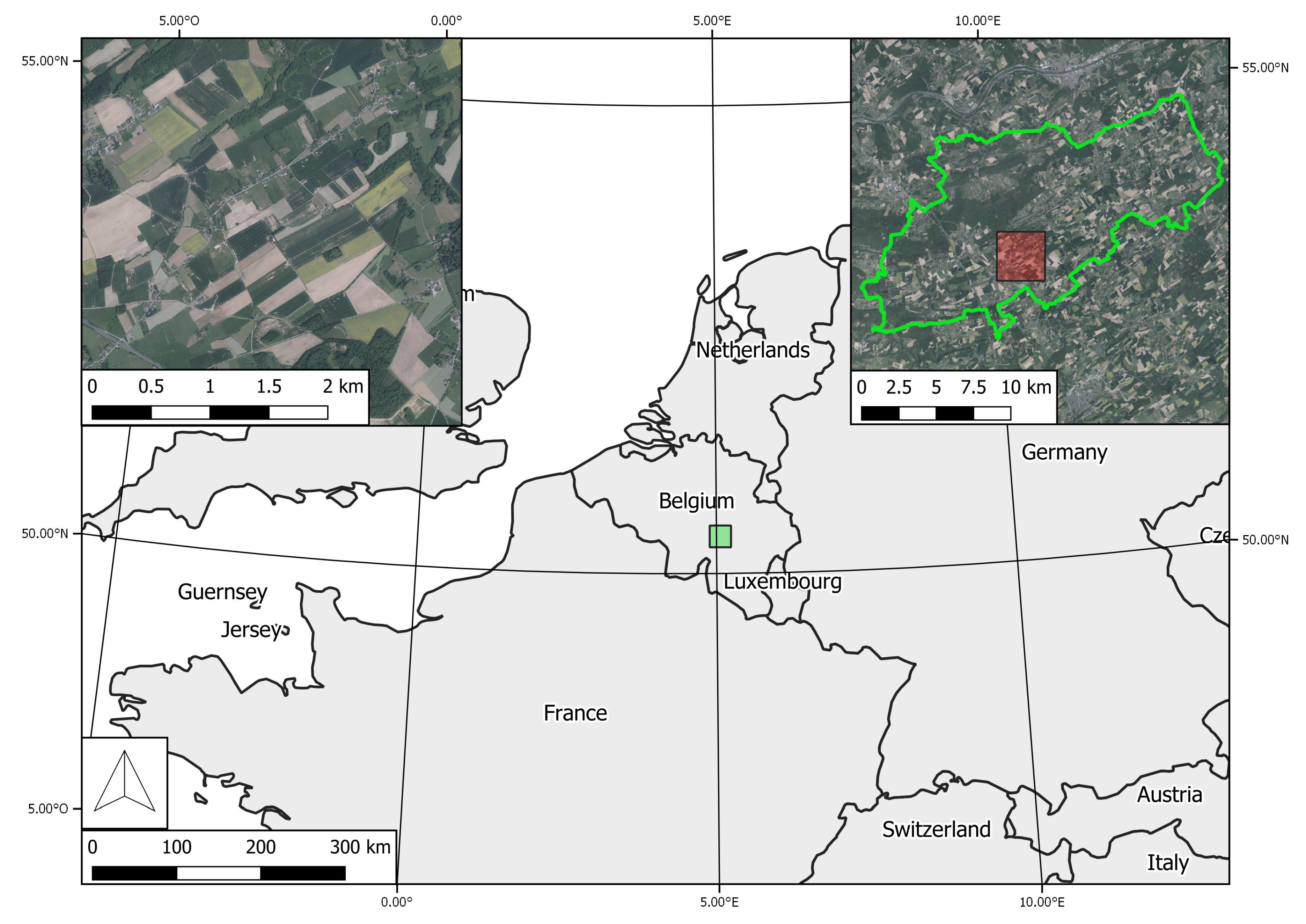
Three adjacent municipalities from southern Belgium were selected as a pilot area (20,076 ha) for this study: Gesves, Assesse, and Ohey (Figure 1). These municipalities combine agricultural and forest contexts and are densely covered by TOF. Table 1 shows the distribution between landcover classes according to the CORINE Land Cover database 2012 (see https://land.copernicus.eu/pan-european/corine-land-cover).
2.2. Remotely Sensed Data
Two publicly available datasets (see http://geoportail.wallonie.be) were used in this study:
- LIDAR data. The study site was covered by two survey flights on 17 December 2013 and 18 January 2014. The average point density of small-footprint discrete airborne LIDAR data was 0.8/m. A canopy height model (CHM) was computed (LIDAR digital surface model—LIDAR digital terrain model) with 1 m ground sampling distance (GSD);
- Orthophotos for which the survey flight took place on 7 June 2013 for the study site. Data were acquired by a VEXCEL UltraCam Xp camera (Vexcel Imaging GmbH, A-8010 Graz, Austria) at 0.25 m GSD. A normalized difference vegetation index (NDVI) was computed at 1 m GSD.
The LIDAR CHM and the NDVI were aligned and stacked into one multiband raster covering the extent of the study site.
2.3. Tools
All the processing steps presented in Section 2 were realized using publicly available software tools. R software [17] was used to develop algorithms and to realize statistical treatments. The package of R [18] was used to develop vector operations. Simple manipulations on raster were realized using the package of R [19]. Advanced processing on raster were realized using the Orfeo Toolbox (OTB) software (see https://www.orfeo-toolbox.org).
2.4. TOF Mapping
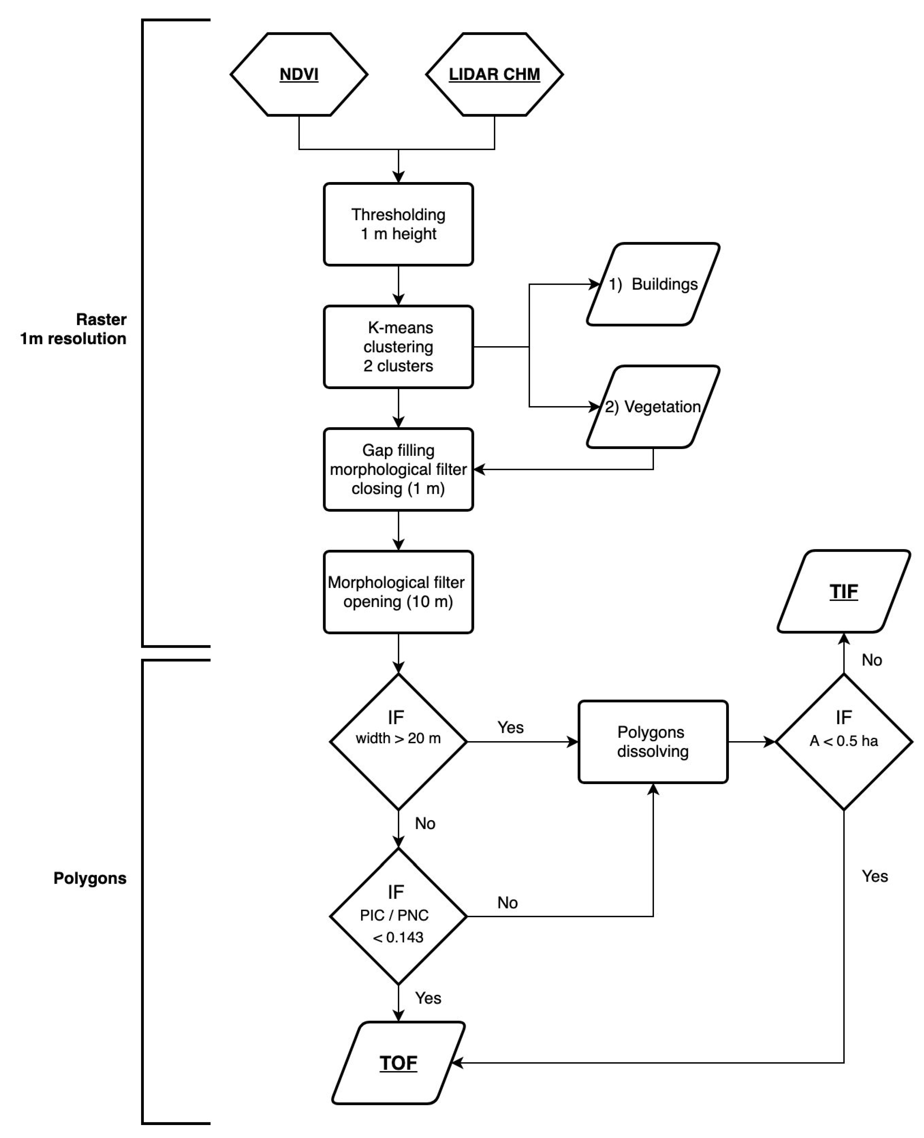
The first part of the processing was applied on raster data (Figure 2, upper part). First, the multi-band raster was masked for LIDAR CHM values smaller than 1 m in height. Through this means, we isolated elevated elements from the ground. Then, an unsupervised classification K-means clustering was applied on the NDVI to separate buildings and vegetation. Only pixels attributed to the cluster grouping higher NDVI values were conserved to make the vegetation raster.
Starting from the vegetation raster, the goal was to conserve only TOF elements. In other words, the elements that did not meet a forest definition were kept. According to the FAO’s definition of forest [20], the forest was defined as a continuous vegetation element larger than 0.5 ha and wider than 20 m.
Small gaps were filled using the binary morphological operation from OTB software (parameters: closing, 1 m in X and Y). The width criterion of the forest definition was tested using a binary morphological operation (parameters: opening, 10 m in X and Y). This processing divided the pixels into two classes: pixels making part of an element wider than 20 m, and pixels making part of an element not wider than 20 m. Afterwards, the raster was polygonized and all subsequent processings were applied to features (Figure 2, bottom).
Polygons not wider than 20 m were subjected to a second test before being classified as TOF. When touching a polygon wider than 20 m, the perimeter in contact (PIC) was compared to the perimeter not in contact with the other polygon (PNC). If the perimeter ratio (PIC/PNC) was lower than 0.143, the polygon was classified as TOF. This value was empirically defined in order to include the elongated polygons in contact with forest. Considering a rectangular element, polygons were considered as elongated if the width/length ratio was smaller than 1/3. For the perimeter ratio (PIC/PNC), it corresponded to 1/7 or 0.143. All polygons with a PIC/PNC ratio higher than 0.143 were dissolved with the polygons in contact.
Afterwards, the area criteria of forest definition was tested on polygons classified wider than 20 m. Polygons smaller than 0.5 ha were classified as TOF. Others were classified as TIF.
2.5. TOF Classification
2.5.1. Targeted TOF Classes
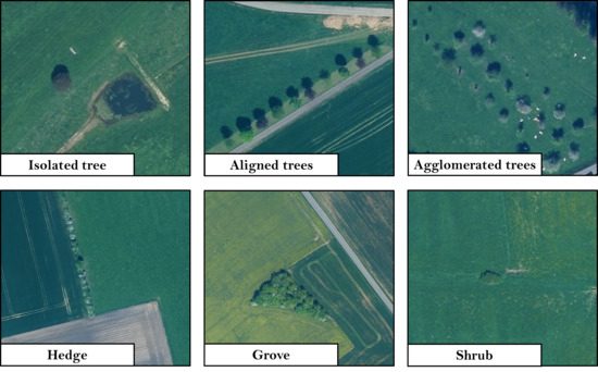
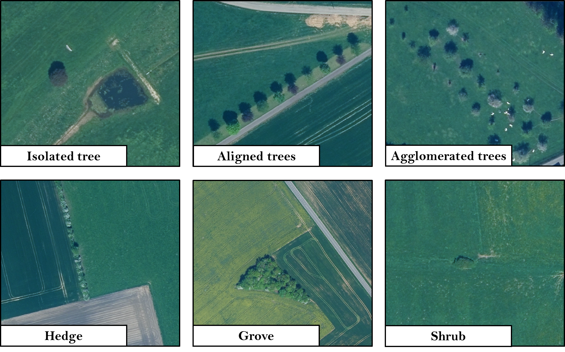
As a European region, the public service of Wallonia (Southern Belgium) has defined control instructions to allocate European agri-environment measures funds. Inspired by its definitions, seven classes were targeted in this paper as being the best compromise between field reality in the European context and a geographic information system (GIS) method. The classes are based on geometric and spatial criteria coming from agri-environment measures definitions adapted for GIS processes. Using GIS, TOF are seen from the sky as crown polygons. According to the following definitions, a woody patch was defined by a nonlinear element having an area smaller than 400 m2:
- Isolated tree: a patch that represents only a single tree crown and that has an area greater than 12.6 m2. For a disk, it corresponds to a diameter of 4 m. The distance between its crown extremity and hedges, groves, and forest is greater than 5 m. The distance between its crown extremity and other patches is larger than 10 m. The circularity (C) is greater than 0.75 ( where A is the area of the polygon, and P is the perimeter);
- Aligned trees: linear group of minimum five patches. The distance between crowns is less than 10 m;
- Agglomerated trees: group of patches not meeting the criteria of aligned trees. The distance between consecutive tree crowns is smaller than 10 m;
- Hedge: linear continuous element with a minimum length (L) of 10 m and a maximum mean width (W) of 20 m. The elongation (E) is higher than 3 ( where E is the elongation, L is the length, and W is the width). Neighboring hedge elements are merged if their distance is less than 5 m;
- Grove: continuous but nonlinear element, the area (A) of which is higher than 400 m2;
- Shrub: patch not assigned to other classes, having a distance of less than 5 m to a neighboring hedge, grove, or forest, and a distance of less than 10 m to a neighboring patch. This class corresponds to shrubs, trees not meeting the criteria to be an isolated tree, and groves smaller than 400 m2;
- Other: TOF not meeting the criteria of any previous definitions.
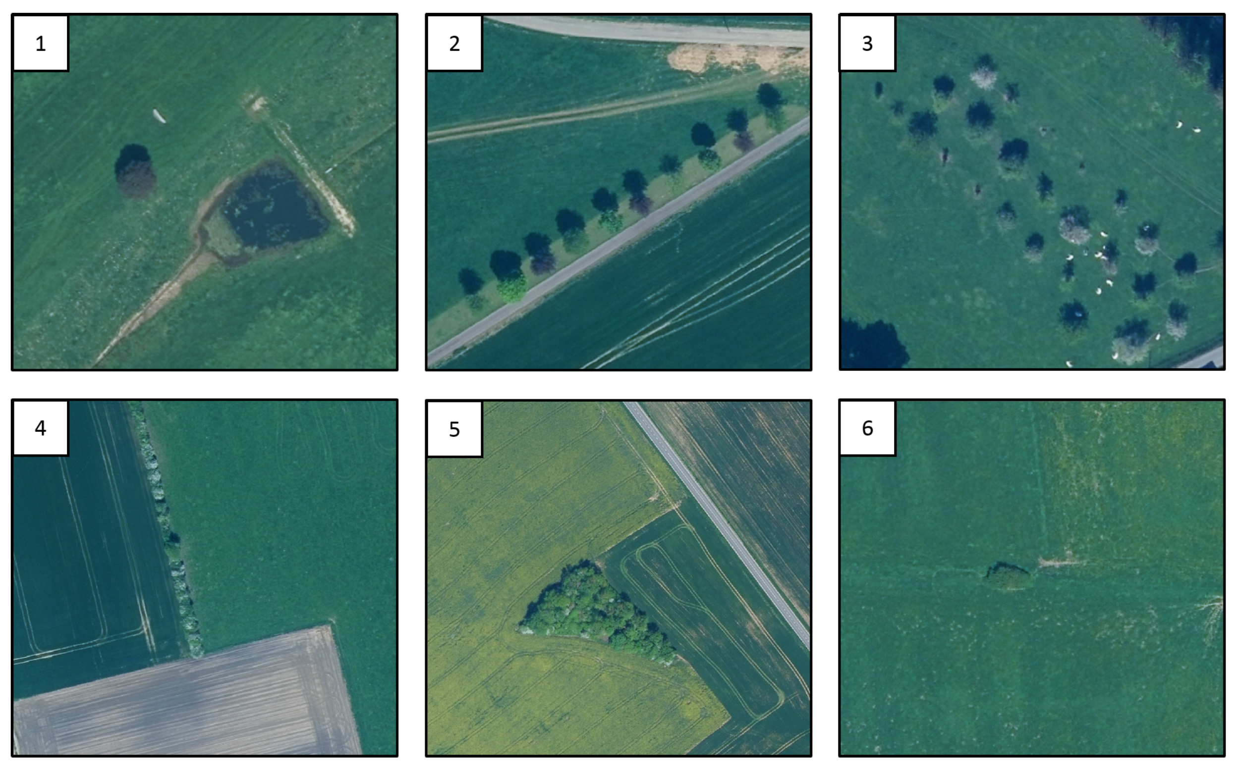
As an example, targeted classes 1 to 6 are illustrated with an orthophoto in Figure 3.
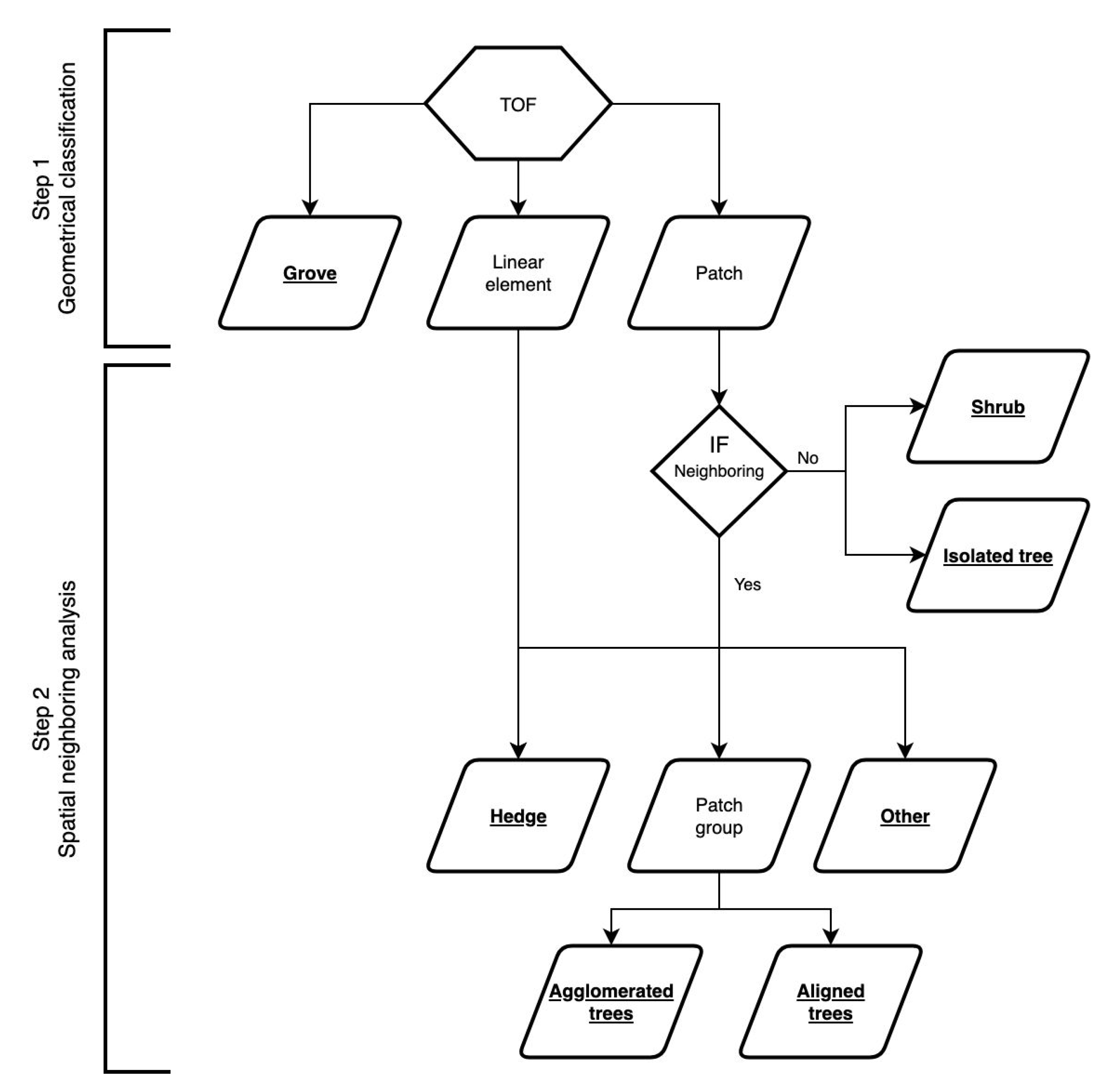
2.5.2. Overall TOF Classification Flowchart
The classification processing was divided into two steps (Figure 4). First, TOF polygons were classified into three geometrical classes: Grove, Linear element, and Patch. Then, the neighboring of Linear elements and Patches was analyzed in order to attribute final TOF classes: Isolated tree, Aligned trees, Agglomerated trees, Hedge, Shrub, and Other.
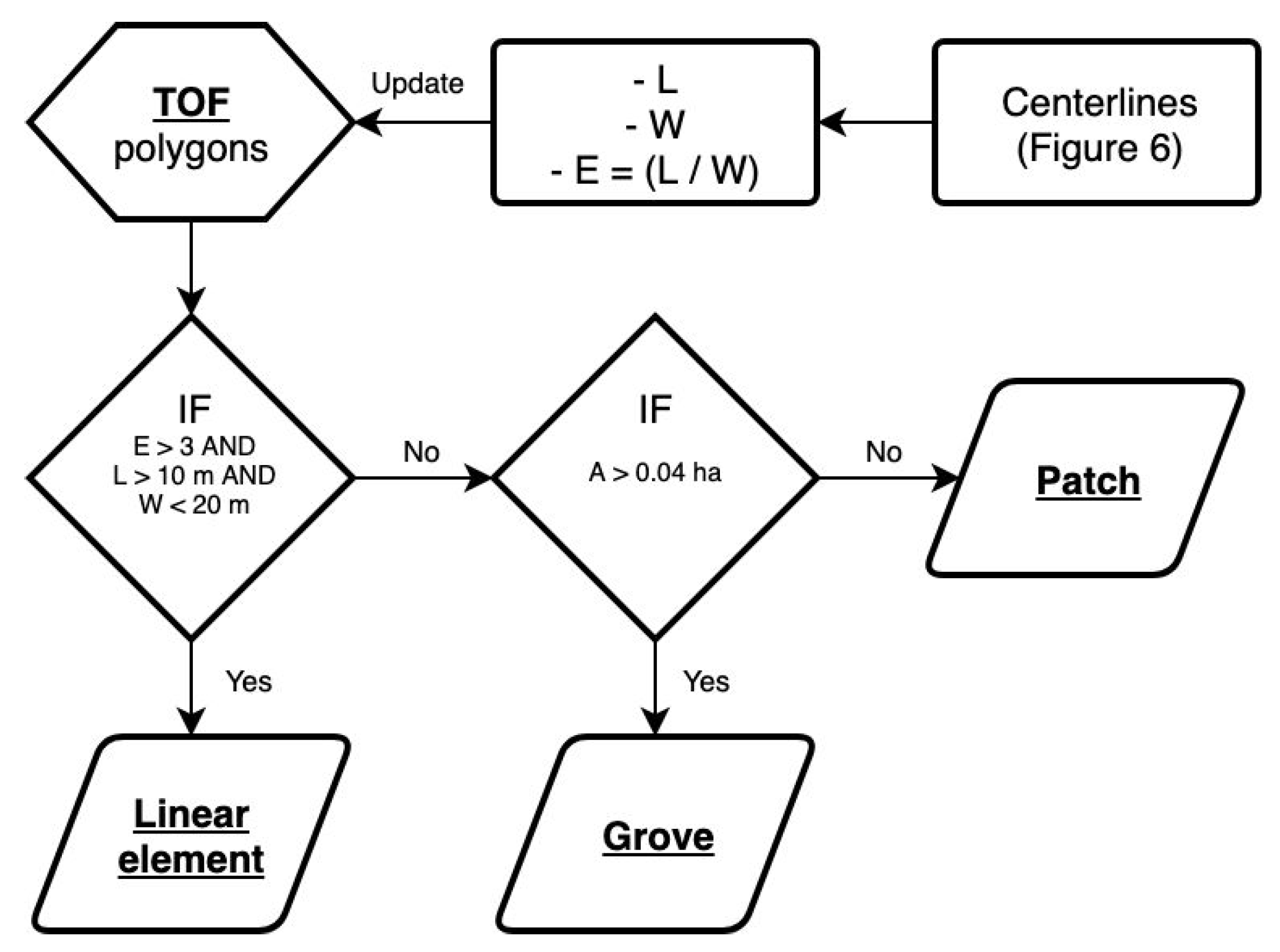
2.5.3. Step 1: Geometrical Classification of TOF Polygons
The goal of this step was to describe the geometry of each TOF polygon based on four parameters: Length (L), Width (W), Elongation (E), and Circularity (C).
Figure 5 describes the classification decisions according to these four parameters. Each polygon was classified into one of the following three classes: Linear element, Grove, and Patch. Among these classes, only the Grove class is a TOF class targeted in this study. Linear element and Patch are intermediate classes that could be combined with another neighboring TOF polygon before the attribution of a targeted class. The analysis of the spatial neighboring is the second step of the TOF classification.
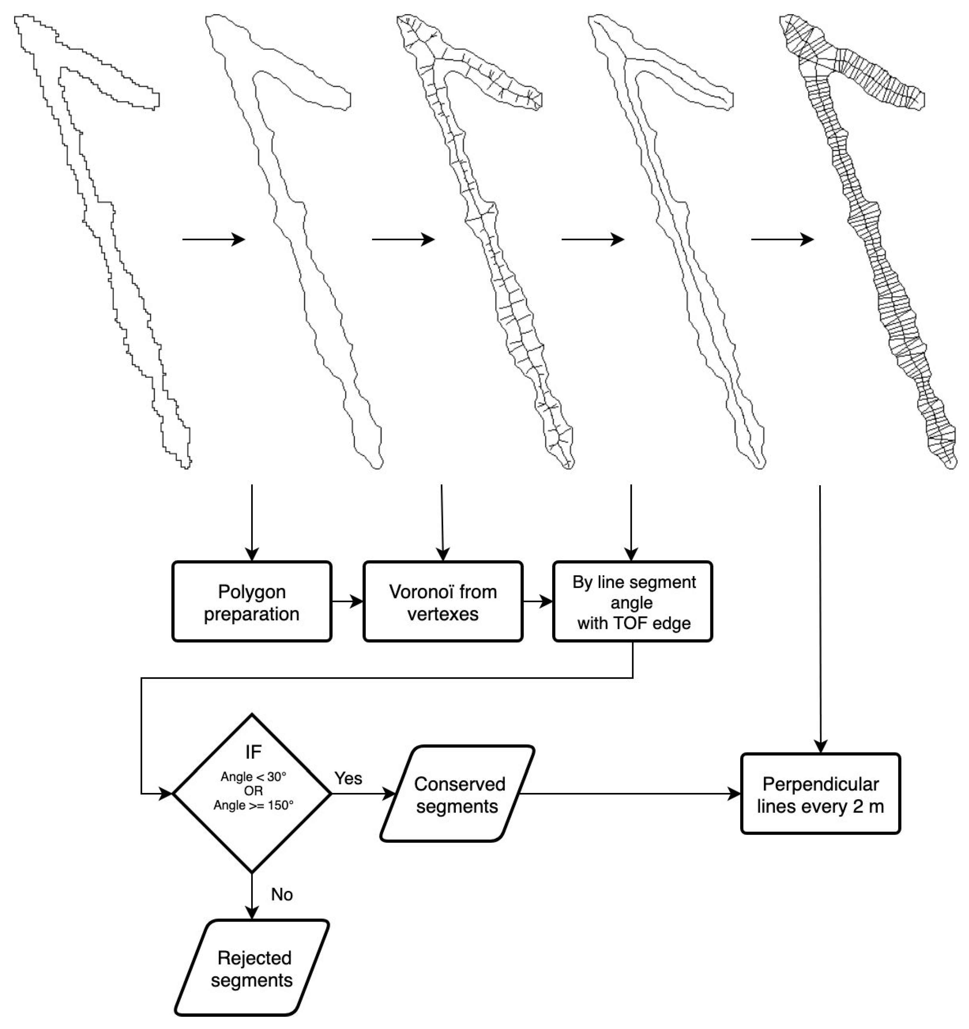
Circularity (C) was computed on smoothed TOF polygons. A positive buffer (+4 m) followed by a negative buffer (−4 m) were applied to smooth the polygon edges formed by 1 m pixel limits. For polygons not wider than 20 m (according to the morphological filter) with circularity lower than 0.5, a centerline was generated in order to evaluate Length (L), Width (W), and Elongation (E). For other polygons, Length, Width, and Elongation were set to 0.
Centerline generation is presented in Figure 6: in addition to the smoothing, TOF polygons were simplified in order to optimize the generation of a skeleton. TOF edges were simplified using the standard Douglas–Peucker algorithm. The tolerance parameter value was set to 0.2 and the preserve topology option was used. By this means, the large number of vertexes was reduced. Furthermore, the edges of the polygons were partitioned into 1-m segments. Then, polygon vertexes were used to generate Voronoi polygons. Voronoi polygon edges were converted into a linestring layer. Only Voronoi edges 0.1 m inside the TOF polygons were conserved.
In order to find the centerline among segments, a filtering process was applied on every line segment. The angle between a line segment and its nearest TOF edge segment (the line formed by two vertexes) was computed. If this angle was greater than 150° or smaller than 30°, it was conserved. Inside a TOF polygon, if the skeleton was cut into several parts after this step, parts were linked by their nearest vertexes. Finally, line segments were merged to create the centerline.
For each TOF centerline segment, perpendicular lines were computed every 2 m and were intersected with their TOF polygon. To avoid estimating width in junctions, perpendicular lines were not conserved when intersecting more than one centerline segment.
For a TOF polygon, Length (L) was computed as the total length of the TOF centerline, and Width (W) was computed as the mean of all the perpendicular line lengths.
2.5.4. Step 2: Spatial Neighboring Analysis
For every feature of the Linear element class and of the Patch class, distances from other features were analyzed from edge to edge. For the Patch class, the potential spatial combinations with other elements in proximity are given in Table 2.
A new class was attributed to Patch TOF having a proximity with these other elements. If several proximities occurred for the same TOF, the order of priority was respected to attribute the new class. For possibilities 1, 2, and 3, the new attributed classes were: Patch group, Hedge, and Other. Thus, a patch near to nothing except the forest or a grove was classified as Other. Furthermore, for possibilities 1 and 2, all the TOF polygons in the same spatial neighboring were grouped into a new multipolygon feature.
Linear element polygons and Hedge multipolygons less than 5 m from each other were grouped into multipolygon features and classified as Hedge.
Patches that were not close to any element were classified as Isolated tree if their area was higher than 12.6 m2 and if Circularity was higher than 0.75. If these two conditions were not met for an isolated Patch, it was classified as Shrub.
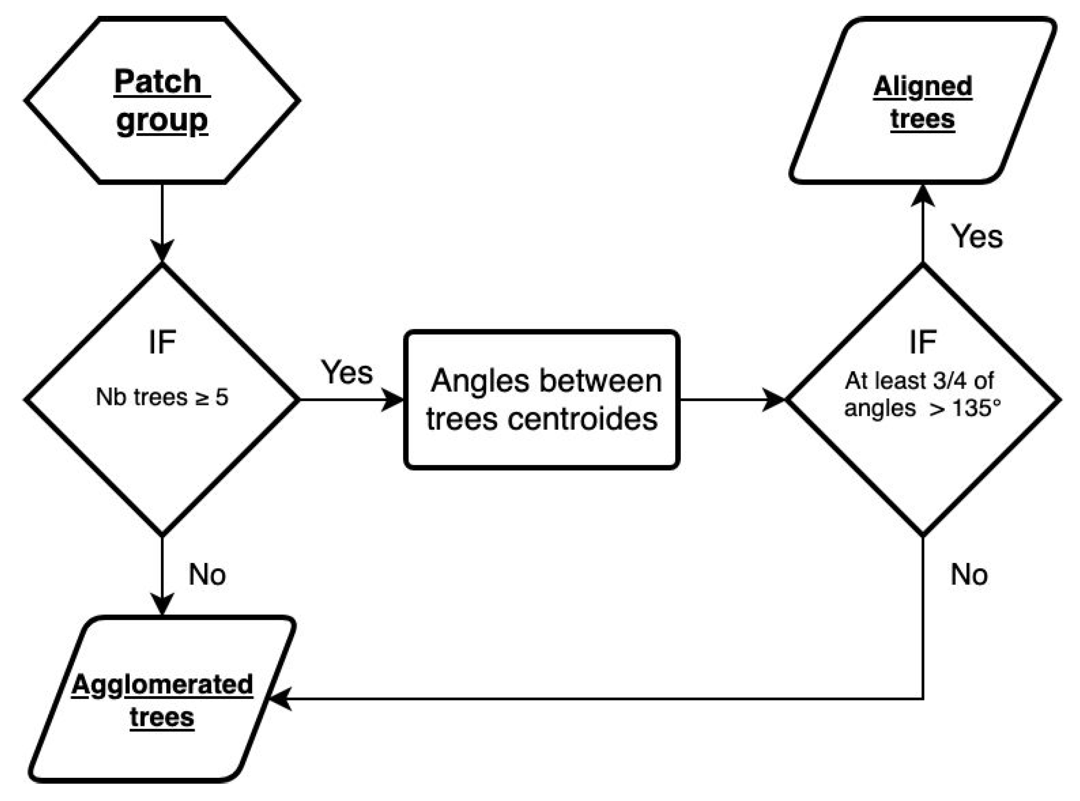
The last treatment classified Patch group multipolygons in two classes: Aligned trees and Agglomerated trees. The number of patches by feature and their aligned disposition were used to make this final classification (Figure 7). The minimum patch number to classify a Patch group into Aligned trees was five. In order to determine if patches were aligned, line segments were generated to link their centroids stepwise, and the angles formed between these segments were then computed. If at least 75% of these angles were greater than 135°, patches were considered as being aligned. For these two classes, the number of patches by feature was saved.
2.5.5. Accuracy Assessment
The TOF classes were primarily designed to inventory TOF agricultural landscapes. For this reason, the accuracy of TOF classification was evaluated in agricultural parcels referenced in the Belgian public database (see http://geoportail.wallonie.be). A visual interpretation of the orthophoto was realized for 10% of the mapped TOF elements located within 5 m of the agricultural parcels layer. The goal was to assess the accuracy of the classification algorithm applied on a TOF map. The accuracy of the TOF mapping was not directly assessed. The 10% sample was randomly selected. Each sample element was visually classified into one class by a skilled operator. If a difference occurred between the automated classification and the visual classification, it was then specified whether the error was due to the TOF classification or to the TOF mapping. Indeed, the TOF classification was based on the geometrical and spatial properties of TOF polygons. Then, if there was some error in the TOF mapping, the algorithm could provide a classification for the polygon which seemed accurate according to its given properties but which was actually erroneous and did not match with the reality observed in the field. When a TOF element was not vegetation but a commission of the TOF map, it was classified as “NO”.
Based on this visual interpretation, a confusion matrix was generated and the overall accuracy was computed. Production (PA) and consumer (CA) accuracies were computed by class. This accuracy assessment was called “complete validation”. Starting from the same dataset, observations with an error associated to the TOF mapping were removed. A second confusion matrix was then generated and accuracy indices (overall accuracy, PA, and CA) were computed. This second accuracy assessment was called “filtered validation”.
3. Results
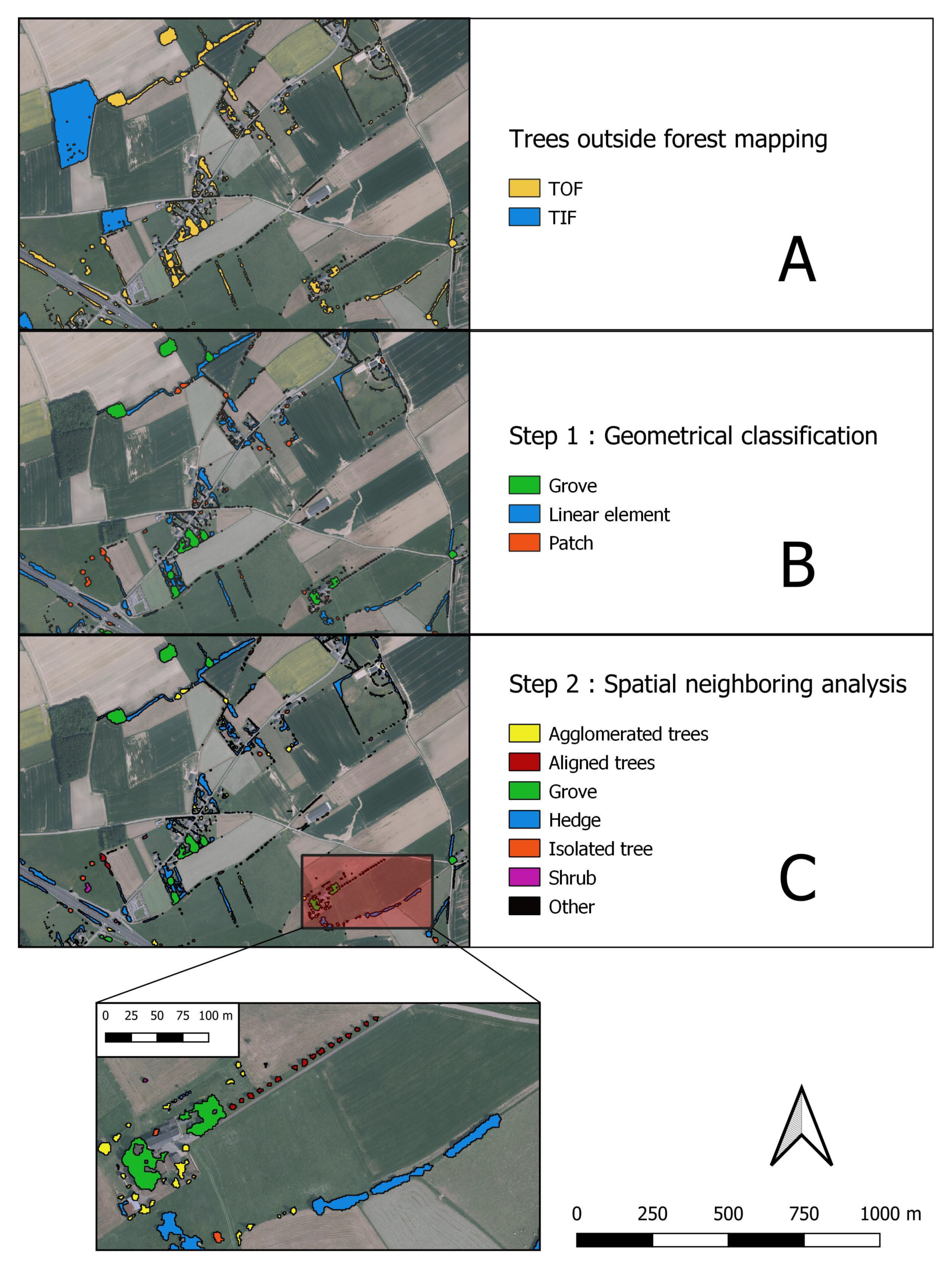
For a visualization zone, Figure 8 shows the results of the TOF mapping as well as those of step 1 and step 2 of the TOF classification.
Table 3 shows areas (ha) covered by the TIF and TOF classes on the study site.
Table 4 shows areas (ha) covered by the targeted classes on the study site.
As shown in Table 5, production accuracies (PAs) and consumer accuracies (CAs) computed with the complete validation were satisfactory. The overall accuracy was 78.4%. The TOF classification was overall conclusive. Nevertheless, the minimum PA was 0.35 for the Aligned trees class and the minimum CA was 0.58 for the Shrub class.
PA and CA were higher for the filtered validation (without errors due to the TOF mapping) with a minimum PA of 0.90 for the Grove class and a minimum CA of 0.89 for the Aligned trees class (Table 5). The overall accuracy was 92.6%. The algorithm of TOF classification made the intended decisions in most cases when considering a reference dataset free from TOF mapping error.
For the complete validation dataset, the overall error of classification was 21.63%; 17.30% were due to the TOF mapping, according to the visual interpretation. The number of validation observations are presented by class in Table 6.
As shown in the confusion matrix built with the complete validation dataset (Table 7), the lowest PA of the Aligned trees class was associated with the confusion with the Agglomerated trees class. The lowest CA of the Shrub class was mainly associated with the confusion with the Agglomerated trees class, the Isolated tree class, and the false detection of vegetation (NO class in Table 7).
4. Discussion
The classification of the seven TOF classes achieved an overall accuracy of 78.4%. This result demonstrates that it is possible to design a fully automated mapping of accurate TOF types that matches the definitions used in field inventories. Accuracies were satisfactory in comparison to similar existing studies. Furthermore, previous studies stopped at step 1 of classification. Using high-resolution satellite imagery, Pujar et al. [16] automatically mapped three TOF classes (Point, Line, and Patch) with an overall accuracy of 75.1% in an agricultural landscape. In their study based on full-waveform laser scanner data, Straub et al. [12] classified four classes: Non-tree vegetation, Forest, Non-forest vegetation—group of trees, Non-forest vegetation—single trees. For the “group of trees” class, the PA was 0.68 and the CA was 0.78. For the “single trees” class, the PA was 0.52 and the CA was 0.69.
The TOF classification deeply depends on TOF polygons’ shape and neighboring. As a consequence, a large part of classification errors were not due to the process itself but to omission, commission, or poor delineations of elements in the TOF mapping. Working on an ideal TOF mask, the developed algorithm predicted the intended class in most cases.
With respect to the aligned trees, the performance of the classification algorithm proved to be highly sensitive to the TOF mapping results. Along an aligned element group, just one missing detection could divide the line into two independent parts no longer meeting the conditions (Figure 7). The worst PA (0.35) of the Aligned trees class confirmed the latter finding (Table 5). Sometimes, aligned trees can be present on both sides of a street. If the street is not wide enough, these two entities were grouped as a single TOF element by the process. A GIS street layer would allow aligned trees to be correctly separated in post-processing in such a case. More generally, the use of an existing GIS layer to test intersection or proximity with structuring elements of the landscape (streets, rivers, etc.) is an interesting perspective to better characterize TOF resources seen from above.
As expected, the most frequent classification error concerned the Shrub class. Indeed, most commissions of TOF detected in the TOF mapping (NO class in Table 7) necessarily had typical properties of the Shrub class as they often corresponded to small but elevated urban elements which can easily be confused with vegetation due to a confusing NDVI signal. Additionally, Agglomerated trees with small height were often classified as Shrub because not all the trees were detected. It appears that the chosen method for vegetation detection is less efficient below a 3-m height and that it produces omissions and poor or incomplete delineations of TOF. Most of the time, this had the effect of classifying separated trees into the Shrub class. Finally, the defined rules applied to differentiate the isolated tree class and the Shrub class are based on an area value and a circularity value. This method appears to be too simple, and it failed in some cases—particularly when the TOF polygon was poorly delineated. More development could be made in order to integrate the certitude that there is one single tree into the existing rules.
In their conclusion, Straub et al. [12] suggested method development in order to classify elongated groups of trees connected with the boundary of the forest as TOF. This was implemented in step 1 through the application of a morphological filter using the distance from the boundary to detect narrow parts of a raster. Nevertheless, this method sometimes revealed unexpected behavior: if there was a gap in the vegetation raster (even as small as one pixel), the distances were then calculated from that gap and the vegetation which was in contact with the gap could be considered as having a width smaller than 20 m while it was actually wider. As a consequence, it could be erroneously classified as TOF.
Separating the vegetation outside the forest in well-defined categories can be regarded as a challenging task. The goal is to reach the best compromise that serves the study objectives. In that way, definitions were built to represent structuring elements of agricultural lands related to agri-environment measures. That is why the results were conclusive in agricultural land, and therefore less adapted to urban areas where the variability of shapes and the number of possible combinations of elements are higher than in agricultural lands. This caused more exceptions and confusion between the defined classes.
5. Conclusions
An accurate and automated classification of trees outside the forest (TOF) that can support the operational management of TOF in rural landscapes was realized. An algorithm was developed for seven classes matching the definitions used in field inventories. The use of the neighboring and possible spatial combinations of TOF elements allowed us to detect complex landscape elements. The overall accuracy of the classification was 78%. This study was entirely carried out by means of publicly available software tools and simple operations in such a way that it improves the reproducibility of the method and shows the potential of geographic information systems and remote sensing for TOF applications. This study demonstrates that automated TOF classification is possible with classes matching the definitions used in field inventories. This suggests that remote sensing has a huge potential to support the operational management of TOF as well as other research areas regarding TOF.
Author Contributions
C.B. and N.L. conceived, designed, and performed the experiments; C.B., P.L., A.M., and N.L. analyzed the data and wrote the paper.
Funding
This research is part of the European Project Interreg V—Forêt Pro Bos portefeuille FeelWood (see https://www.foret-pro-bos.eu), and received financial support from the same.
Acknowledgments
The authors thank Thibault Delinte who performed the visual interpretation used in accuracy assessment.
Conflicts of Interest
The authors declare no conflict of interest. The founding sponsors had no role in the design of the study; in the collection, analyses, or interpretation of data; in the writing of the manuscript; or in the decision to publish the results.
Abbreviations
The following abbreviations are used in this manuscript:
| A | Area |
| ALS | Airborne laser scanning |
| C | Circularity |
| CHM | Canopy height model |
| CA | Consumer accuracy |
| E | Elongation |
| FAO | Food and Agriculture Organization of the United Nations |
| GIS | Geographic information system |
| GSD | Ground sampling distance |
| L | Length |
| NDVI | Normalized Difference Vegetation Index |
| OTB | Orfeo Toolbox software |
| PA | Production accuracy |
| PIC | Perimeter in contact |
| PNC | Perimeter not in contact |
| TIF | Trees in the forest |
| TOF | Trees outside the forest |
| W | Width |
References
- Schnell, S.; Altrell, D.; Ståhl, G.; Kleinn, C. The contribution of trees outside forests to national tree biomass and carbon stocks—A comparative study across three continents. Environ. Monit. Assess. 2015, 187. [Google Scholar] [CrossRef] [PubMed]
- Zomer, R.J.; Neufeldt, H.; Xu, J.; Ahrends, A.; Bossio, D.; Trabucco, A.; van Noordwijk, M.; Wang, M. Global Tree Cover and Biomass Carbon on Agricultural Land: The contribution of agroforestry to global and national carbon budgets. Sci. Rep. 2016, 6. [Google Scholar] [CrossRef] [PubMed]
- McCollin, D.; Jackson, J.; Bunce, R.; Barr, C.; Stuart, R. Hedgerows as habitat for woodland plants. J. Environ. Manag. 2000, 60, 77–90. [Google Scholar] [CrossRef]
- Rossi, J.P.; Garcia, J.; Roques, A.; Rousselet, J. Trees outside forests in agricultural landscapes: Spatial distribution and impact on habitat connectivity for forest organisms. Landsc. Ecol. 2016, 31, 243–254. [Google Scholar] [CrossRef]
- FAO members adopt first global action plan for forest genetic resources. Unasylva 2013, 64, 72–74.
- Schnell, S.; Kleinn, C.; Ståhl, G. Monitoring trees outside forests: A review. Environ. Monit. Assess. 2015, 187. [Google Scholar] [CrossRef] [PubMed]
- Marchetti, M.; Garfì, V.; Pisani, C.; Franceschi, S.; Marcheselli, M.; Corona, P.; Puletti, N.; Vizzarri, M.; di Cristofaro, M.; Ottaviano, M.; Fattorini, L. Inference on forest attributes and ecological diversity of trees outside forest by a two-phase inventory. Ann. For. Sci. 2018, 75, 37. [Google Scholar] [CrossRef]
- Plieninger, T.; Schleyer, C.; Mantel, M.; Hostert, P. Is there a forest transition outside forests? Trajectories of farm trees and effects on ecosystem services in an agricultural landscape in Eastern Germany. Land Use Policy 2012, 29, 233–243. [Google Scholar] [CrossRef] [Green Version]
- Plieninger, T. Monitoring directions and rates of change in trees outside forests through multitemporal analysis of map sequences. Appl. Geogr. 2012, 32, 566–576. [Google Scholar] [CrossRef] [Green Version]
- Seidel, D.; Busch, G.; Krause, B.; Bade, C.; Fessel, C.; Kleinn, C. Quantification of Biomass Production Potentials from Trees Outside Forests—A Case Study from Central Germany. Bioenergy Res. 2015, 8, 1344–1351. [Google Scholar] [CrossRef]
- Seidel, D.; Hähn, N.; Annighöfer, P.; Benten, A.; Vor, T.; Ammer, C. Assessment of roe deer (Capreolus capreolus L.) – vehicle accident hotspots with respect to the location of ‘trees outside forest’ along roadsides. Appl. Geogr. 2018, 93, 76–80. [Google Scholar] [CrossRef]
- Straub, C.; Weinacker, H.; Koch, B. A fully automated procedure for delineation and classification of forest and non-forest vegetation based on full waveform laser scanner data. Int. Arch. Photogramm. Remote Sens. Spat. Inf. Sci. 2008, 37, 1013–1019. [Google Scholar]
- Maack, J.; Lingenfelder, M.; Eilers, C.; Smaltschinski, T.; Weinacker, H.; Jaeger, D.; Koch, B. Estimating the spatial distribution, extent and potential lignocellulosic biomass supply of Trees Outside Forests in Baden-Wuerttemberg using airborne LiDAR and OpenStreetMap data. Int. J. Appl. Earth Observ. Geoinf. 2017, 58, 118–125. [Google Scholar] [CrossRef]
- Meneguzzo, D.; Liknes, G.; Nelson, M. Mapping trees outside forests using high-resolution aerial imagery: A comparison of pixel- and object-based classification approaches. Environ. Monit. Assess. 2013, 185, 6261–6275. [Google Scholar] [CrossRef] [PubMed]
- Singh, K.; Chand, P. Above-ground tree outside forest (TOF) phytomass and carbon estimation in the semi-arid region of southern Haryana: A synthesis approach of remote sensing and field data. J. Earth Syst. Sci. 2012, 121, 1469–1482. [Google Scholar] [CrossRef]
- Pujar, G.; Reddy, P.; Reddy, C.; Jha, C.; Dadhwal, V. Estimation of trees outside forests using IRS high resolution data by object based image analysis. Int. Arch. Photogramm. Remote Sens. Spat. Inf. Sci. 2014, 40, 623–629. [Google Scholar] [CrossRef]
- R Core Team. R: A Language and Environment for Statistical Computing; R Foundation for Statistical Computing: Vienna, Austria, 2018. [Google Scholar]
- Pebesma, E. Simple Features for R: Standardized Support for Spatial Vector Data. The R Journal. 2018. Available online: https://journal.r-project.org/archive/2018/RJ-2018-009/ (accessed on 18 March 2019).
- Hijmans, R.J. Raster: Geographic Data Analysis and Modeling. R package Version 2.8-4. 2018. Available online: https://CRAN.R-project.org/package=raster (accessed on 18 March 2019).
- FAO. FRA 2015 Terms and Definitions; FAO: Rome, Italy, 2015. [Google Scholar]
Figure 1.
Localisation of the study site (green square). The study site edges (green lines) are shown in the top-right corner (orthophoto 2012–2013, Public service of Wallonia). A more detailed view is presented in the top-left corner, located by the red square in the top-right corner view.
Figure 1.
Localisation of the study site (green square). The study site edges (green lines) are shown in the top-right corner (orthophoto 2012–2013, Public service of Wallonia). A more detailed view is presented in the top-left corner, located by the red square in the top-right corner view.

Figure 2.
Flowchart of the trees outside the forest (TOF) mapping. CHM: canopy height model; NDVI: normalized difference vegetation index; TIF: trees in the forest.
Figure 2.
Flowchart of the trees outside the forest (TOF) mapping. CHM: canopy height model; NDVI: normalized difference vegetation index; TIF: trees in the forest.

Figure 3.
Illustration of the targeted classes for the TOF classification: 1: Isolated tree, 2: Aligned trees, 3: Agglomerated trees, 4: Hedge, 5: Grove, 6: Shrub. Orthophoto 2018, Public service of Wallonia.
Figure 3.
Illustration of the targeted classes for the TOF classification: 1: Isolated tree, 2: Aligned trees, 3: Agglomerated trees, 4: Hedge, 5: Grove, 6: Shrub. Orthophoto 2018, Public service of Wallonia.

Figure 4.
Overall flowchart of the TOF classification divided into two steps: geometrical classification and spatial neighboring analysis. Targeted classes are marked in bold and underlined.
Figure 4.
Overall flowchart of the TOF classification divided into two steps: geometrical classification and spatial neighboring analysis. Targeted classes are marked in bold and underlined.

Figure 5.
Flowchart of the first step of classification: geometrical classification of TOF polygons.
Figure 5.
Flowchart of the first step of classification: geometrical classification of TOF polygons.

Figure 6.
Flowchart of the centerline generation.

Figure 7.
Flowchart of the Patch groups classification into two classes: Aligned trees and Agglomerated trees.
Figure 7.
Flowchart of the Patch groups classification into two classes: Aligned trees and Agglomerated trees.

Figure 8.
Visualization zone of the results. (A) the trees outside the forest mapping. Two classes in the legend: trees outside the forest (TOF) and trees in the forest (TIF); (B) step 1 of the TOF classification—geometrical classification of TOF polygons; (C) step 2 of the TOF classification—spatial neighboring analysis. For step 2, a more detailed view is presented on the bottom. Background map: orthophoto 2012–2013, Public service of Wallonia.


Table 1.
Distribution of areas (ha) by land cover class according to the CORINE Land Cover database 2012.
Table 1.
Distribution of areas (ha) by land cover class according to the CORINE Land Cover database 2012.
| Land Cover | Area (ha) |
|---|---|
| Agricultural areas | 13,057.80 |
| Artificial surfaces | 2605.73 |
| Forest and semi-natural areas | 4411.99 |
Table 2.
Spatial combinations for the Patch class, in decreasing order of priority.
| Neighboring Test | 1. Patch 10 m Around | 2. Linear Element 5 m Around | 3. Forest or Grove 5 m Around |
|---|---|---|---|
| New class | Patch group | Hedge | Other |
Table 3.
Areas (ha) covered by trees in the forest (TIF) and trees outside the forest (TOF) on the study site.
Table 3.
Areas (ha) covered by trees in the forest (TIF) and trees outside the forest (TOF) on the study site.
| Class | Area (ha) |
|---|---|
| TIF | 5169.35 |
| TOF | 1040.65 |
Table 4.
Distribution of areas (ha) by targeted class on the study site.
| Class | Area (ha) |
|---|---|
| Agglomerated trees | 74.26 |
| Aligned trees | 2.35 |
| Grove | 339.16 |
| Hedge | 596.58 |
| Isolated tree | 9.75 |
| Other | 6.28 |
| Shrub | 12.27 |
Table 5.
Production accuracies (PAs) and consumer accuracies (CAs) of the classification by TOF class, computed for the complete validation dataset and the filtered validation dataset.
Table 5.
Production accuracies (PAs) and consumer accuracies (CAs) of the classification by TOF class, computed for the complete validation dataset and the filtered validation dataset.
| PA | CA | |||
|---|---|---|---|---|
| Complete | Filtered | Complete | Filtered | |
| Agglomerated trees | 0.79 | 0.98 | 0.80 | 0.97 |
| Aligned trees | 0.35 | 1.00 | 0.73 | 0.89 |
| Grove | 0.78 | 0.90 | 0.95 | 0.97 |
| Hedge | 0.86 | 0.95 | 0.85 | 0.93 |
| Isolated tree | 0.76 | 0.99 | 0.83 | 0.92 |
| Other | 0.92 | 0.92 | 0.76 | 0.97 |
| Shrub | 0.90 | 0.92 | 0.58 | 0.95 |
Table 6.
Number of observations by class in complete and filtered validation datasets.
| Agglomerated Trees | Aligned Trees | Grove | Hedge | Isolated Tree | Other | Shrub | Total | |
|---|---|---|---|---|---|---|---|---|
| Complete | 266 | 11 | 122 | 335 | 124 | 45 | 253 | 1156 |
| Filtered | 220 | 9 | 120 | 305 | 112 | 35 | 155 | 956 |
Table 7.
Confusion matrix of the TOF classification, built with the complete validation dataset. Observations are sorted by reference class in columns, and by prediction class in rows.
Table 7.
Confusion matrix of the TOF classification, built with the complete validation dataset. Observations are sorted by reference class in columns, and by prediction class in rows.
| Prediction | Reference | |||||||
|---|---|---|---|---|---|---|---|---|
| Agglomerated Trees | Aligned Trees | Grove | Hedge | Isolated Tree | NO | Other | Shrub | |
| Agglomerated trees | 213 | 12 | 1 | 27 | 1 | 8 | 0 | 4 |
| Aligned trees | 1 | 8 | 0 | 2 | 0 | 0 | 0 | 0 |
| Grove | 3 | 0 | 116 | 3 | 0 | 0 | 0 | 0 |
| Hedge | 10 | 1 | 28 | 285 | 0 | 5 | 3 | 3 |
| Isolated tree | 5 | 0 | 1 | 2 | 103 | 4 | 0 | 9 |
| NO | 0 | 0 | 0 | 0 | 0 | 0 | 0 | 0 |
| Other | 5 | 0 | 3 | 1 | 0 | 1 | 34 | 1 |
| Shrub | 32 | 2 | 0 | 11 | 31 | 30 | 0 | 147 |
© 2019 by the authors. Licensee MDPI, Basel, Switzerland. This article is an open access article distributed under the terms and conditions of the Creative Commons Attribution (CC BY) license (http://creativecommons.org/licenses/by/4.0/).
Share and Cite
MDPI and ACS Style
Bolyn, C.; Lejeune, P.; Michez, A.; Latte, N. Automated Classification of Trees outside Forest for Supporting Operational Management in Rural Landscapes. Remote Sens. 2019, 11, 1146. https://doi.org/10.3390/rs11101146
AMA Style
Bolyn C, Lejeune P, Michez A, Latte N. Automated Classification of Trees outside Forest for Supporting Operational Management in Rural Landscapes. Remote Sensing. 2019; 11(10):1146. https://doi.org/10.3390/rs11101146
Chicago/Turabian StyleBolyn, Corentin, Philippe Lejeune, Adrien Michez, and Nicolas Latte. 2019. "Automated Classification of Trees outside Forest for Supporting Operational Management in Rural Landscapes" Remote Sensing 11, no. 10: 1146. https://doi.org/10.3390/rs11101146
Note that from the first issue of 2016, this journal uses article numbers instead of page numbers. See further details here.