Automatic Ship Detection in Optical Remote Sensing Images Based on Anomaly Detection and SPP-PCANet


1
Beijing Key Laboratory of Digital Media, School of Computer Science and Engineering, Beihang University, Beijing 100191, China
2
State Key Laboratory of Virtual Reality Technology and Systems, Beihang University, Beijing 100191, China
*
Author to whom correspondence should be addressed.
Remote Sens. 2019, 11(1), 47; https://doi.org/10.3390/rs11010047
Submission received: 15 November 2018
/
Revised: 21 December 2018
/
Accepted: 25 December 2018
/
Published: 29 December 2018
(This article belongs to the Special Issue Pattern Analysis and Recognition in Remote Sensing)
Abstract
:Automatic ship detection technology in optical remote sensing images has a wide range of applications in civilian and military fields. Among most important challenges encountered in ship detection, we focus on the following three selected ones: (a) ships with low contrast; (b) sea surface in complex situations; and (c) false alarm interference such as clouds and reefs. To overcome these challenges, this paper proposes coarse-to-fine ship detection strategies based on anomaly detection and spatial pyramid pooling pcanet (SPP-PCANet). The anomaly detection algorithm, based on the multivariate Gaussian distribution, regards a ship as an abnormal marine area, effectively extracting candidate regions of ships. Subsequently, we combine PCANet and spatial pyramid pooling to reduce the amount of false positives and improve the detection rate. Furthermore, the non-maximum suppression strategy is adopted to eliminate the overlapped frames on the same ship. To validate the effectiveness of the proposed method, GF-1 images and GF-2 images were utilized in the experiment, including the three scenarios mentioned above. Extensive experiments demonstrate that our method obtains superior performance in the case of complex sea background, and has a certain degree of robustness to external factors such as uneven illumination and low contrast on the GF-1 and GF-2 satellite image data.
1. Introduction
In recent decades, research on Synthetic Aperture Radar (SAR) images [1,2,3] has improved considerably, taking advantage of insensitivity in time and weather. However, low resolution and monochrome SAR images can result in the lack of target texture and color features. In addition, despite the visibility of disturbances (wakes) of water surface in SAR images, the characteristics of the ship itself can be invisible, resulting in missed detection. Compared with SAR images, optical images have more detailed information and more obvious geometric structures. This means that optical images can capture more details and complex structures of observation scenes, and can be further used for target recognition. In view of these advantages, ships in optical remote sensing images are often regarded as research targets. Ship detection of marine in optical remote sensing image has a paramount application value in military and civilian fields. The main applications in the military field include battlefield environmental assessment and terrorist activity surveillance. Finding the ship target of interest quickly from many optical remote sensing images is a technical prerequisite for tracking, locating, and identifying a ship. In the civilian sector, attention is paid to the location of passing ships within the target sea area to improve marine administration, thus playing an important role in maritime traffic, safety, and rescue. Therefore, ship target detection is of great significance to optical imaging satellites in marine monitoring.
Traditional object detection is generally divided into two steps: searching and classification. More specifically, a sliding window is used to determine the location of an object, and then the features in this window and shadow classifiers [4] have to be manually designed for further classification [5]. Gradually, methods based on deep neural networks [6] have been proposed successively, which include the steps of labeling raw data and training neural networks. Compared with the traditional method, deep learning methods are more effective and faster for target detection. In the natural image processing for target detection schemes, researchers have successively proposed some target detection techniques, such as RCNN [7], Fast-RCNN [8], Faster-RCNN [9], R-FCN [10], YOLO [11], SSD [12], FPN [13], Mask-RCNN [14], Focal Loss [15] and other deep learning algorithm frameworks. These methods can be used to train outstanding detection models in the public dataset of natural images. However, in the field of ship detection of remote sensing images, the use of the above-mentioned methods has been less impressive in that there is a lack of published datasets with ground truth marks. In the military, the ship dataset is confidential. Moreover, the acquisition of some datasets with ground truth is also limited. Some scholars [16,17,18,19] have labeled ground truth for their own datasets, but these datasets are not used publicly. A fact that cannot be ignored is that manually annotated sample costs are relatively high. Furthermore, there is a difference in imaging mechanism between remote sensing images and natural images, so that in some ways training target recognition algorithms in the dataset of natural images cannot be well applied to remote sensing images. Most importantly, if the target data are not similar to the original data, more challenging work is needed to rough tune or fine tune the neural network when the methods mentioned above are used to load the pre-training model for transfer learning.
To improve the speed and accuracy of ship detection, some coarse-to-fine detection algorithms have been designed [20,21,22]. In recent years, the extraction approaches of ship candidate areas have been proposed, for example, bayesian decision (BD) [23], compressed domain [24], and convolutional neural network [16,25]. In addition, the sparse feature method based on multi-layer sparse coding [26,27,28,29,30] was used to segment the saliency map [21,31,32] to obtain candidate regions. An effective multi scale CFAR detector for the gamma distribution clutter model [33] was also designed to detect candidate targets in the sea. Extended wavelet transform (EWT) was combined with phase saliency map [34] to extract regions of interest (ROI). Simultaneously, in the phase of elimination of false alarms in fine detection, ship detection algorithms have witnessed significant progress. LBP features are extracted from the literature [35,36]. A compressed-domain of the ship detection framework [24] is proposed by means of combining with deep neural network (DNN) and extreme learning machine (ELM). DNN is exploited for high-level feature representation and classification, and ELM is used for efficient feature pooling and decision making. Previous studies [37,38] exclude false alarms by using SVM. Classification algorithms by employing the features of colors, textures and local shapes for ship detection are introduced in [39,40]. Adopting a sparsely-encoded of bag-word model, Sun et al. [41] proposed an automatic target detection framework. The visual saliency model is successively proposed in [42,43]. A multitude of studies [44,45] indicate that the performance of the ship detection system can be improved by combining previous methods. The maximum likelihood (ML) discrimination algorithm [33] is also exploited to further eliminate false alarms.
In some relatively simple conditions, the methods mentioned above can achieve considerable detection results. However, the detection performance of these algorithms will be affected in the following three situations: (a) low contrast between ships and background; (b) scenes with complicated sea conditions, such as large waves and uneven illumination; and (c) false alarm interference, such as clouds, reefs, harbors and islands. In addition, these algorithms also give rise to different levels of missed detection when multiple vessels are docked. Therefore, there is still much room for improvement in ship detection algorithms.
In general, the ship detection methods can be divided into two-stage and one-stage detectors, employing a coarse-to-fine strategy [26,27]. A phase detector, inputs the original image and directly outputs the detection result. Combining the mechanism analysis, experience and knowledge, we adopt two-stage detection techniques in this paper mainly because one-stage detectors have lower accuracy than two-stage detectors. As shown in the previous research, the two main challenges for ship target detection are the extraction of candidate regions in a complex context and the identification of targets when they are similar to false alarm. This method thus utilizes the anomaly detection technology based on the multivariate Gaussian distribution to extract the candidate region (coarse detection). This technology can effectively narrow the subsequent search area and reduce the missed detection rate. Then, the slice of the candidate region is set to a fixed size, which is used as an input of the PCANet network to perform feature training and extraction. In addition, to reduce the missed detection rate, we add spatial pyramid pooling (SPP) at the output layer of PCANet. The SPP allows the images of the training phase to be of various sizes and scales so that the deformation of the object is robust. Training with images of various sizes can improve scale invariance and reduce the occurrence of over fitting. Afterwards, the features extracted by the above stages are then fed into the LibSVM for classification. Due to the addition of SPP, extra overlapping boxes are generated, and we use non-maximum suppression (NMS) to exclude overlapping boxes in false alarms. The fine detection stage effectively screens out accurate vessels from candidate areas, which are roughly detected in the previous stage, further eliminating false alarms and improving the accuracy of detection. By combining the above two stages, the method proposed in this paper can excellently detect the target in the three challenging situations mentioned above.
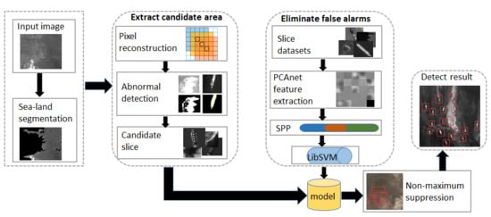
The organization of this paper is as follows. In Section 2, the method adopted is presented, including the anomaly detection based on the multivariate Gaussian distribution to determine the target candidate area. In addition, the algorithm based on SPP-PCANet and LibSVM is described, which extracts and classifies features, and the NMS strategy is discussed, which can eliminate redundant overlapping boxes. The experimental studies are introduced to verify the proposed method in Section 3. Section 4 contains conclusions and further work. The overall flow chart of the method proposed in this paper is shown in Figure 1.
2. Methodology
The ship detection framework adopted by this paper consists of three consecutive phases: pre-processing, pre-screening and discrimination.
2.1. Preprocessing: Sea and Land Segmentation
The quality of the candidate area directly affects the accuracy of the target detection task. To extract fewer high-quality pre-selected windows without redundancy, sea–land image segmentation is performed by using GIS information before anomaly detection. The above operation not only accelerates the speed of target detection, but also improves the performance of target detection and recall rate. The results of the sea–land segmentation experiment are shown in Figure 2.
First, the segmentation results of the image blocks of the land and sea boundaries are coordinated with the GIS library information of the corresponding location. The coordinate solving error is corrected according to the sliding mean value with the maximum matching degree, and then the binary image of the sea–land segmentation is obtained, in which the ocean region is 1 (white) and the land region is 0 (black). Subsequently, the original image is convoluted with the binary image that obtained after the sea–land segmentation, so we get a sea–land segmentation map in which the ocean region exists in the original image. The matching degree is calculated by the following formula.
where Fitting(R) is the matching degree of the binary graph R obtained by image segmentation, is the pixel value of the ith row and the jth column in the binary image, and is a binary map obtained by the sliding window in the GIS library.
2.2. Pre-Screening: Anomaly Detection Algorithm
(a) Maximum interclass variance method
The maximum interclass variance method is also known as the Otsu algorithm, which is derived from the principle of least squares based on gray histogram. The basic rule of the algorithm is to divide the gray value of the image into two parts with the optimal threshold, so that the variance between the two parts is the largest, i.e., the maximum separation. In view of this, the interclass variance of the background and target in the image can be expressed as follows:
where k is the gray level and is the total average gray value of the image. In addition, and represent the average gray value of the background and target parts, respectively, and and are the probabilities of occurrence of the background and the target part. By calculating the inter-class variance at different k values, the corresponding k is the optimal threshold required when reaches the maximum.
(b) Iterative threshold segmentation
The algorithm uses an iterative method to find the optimal threshold for segmentation. First, the parameter is set and an initial estimated threshold is selected. Then, the image is divided into two parts and by the threshold as shown in the following formula:
where represents a portion whose gray value is greater than and represents a part with gray value is less than or equal to . Finally, we calculate the average gray values and of all the pixels in and , respectively, and the new threshold where . The best segmentation threshold can be found if the following conditions are met:
If these above conditions are satisfied, is the optimal threshold ; otherwise, is assigned to , and the above steps are repeated until the optimal threshold is obtained.
(c) Multivariate Gaussian distribution model
In general, the principle of the anomaly detection algorithm is that the number of negative samples is much higher than that of positive samples, so that the parameters of Gaussian model can be fitted with negative samples. The value of is larger for normal samples and smaller for abnormal samples. Since ships (as positive samples) are less accounted for in large proportion of the background ocean (as negative samples) in optical remote sensing images, which satisfies the conditions of abnormality detection, the ship can be detected as an abnormality. Multivariate Gaussian distribution model (Formula (5)) can automatically capture the correlation between different feature variables and identify them as abnormal when the combination is not normal. Moreover, the number of samples is required to be greater than the number of characteristic variables within the multivariate Gaussian distribution, which is not very suitable for n large cases. This is to ensure that the covariance matrix is reversible and there are enough data to fit the parameters in the .
where is an n-dimensional mean vector and covariance is an matrix. If the following condition is met, it is considered to be an abnormal part.
We follow the strategy of moving the window from left to right and top to bottom to rearrange the pixels of each window size. Assuming that the input image size is , the sample is constructed using a sliding window of size so that each sample is a vector. More intuitively, each pixel is the center of its corresponding sliding window in the final image size of . When each pixel is replaced by a vector in the sliding window, a new sample set of is formed, which we denote as . Among them, s is the step size of the sliding window, and we take it as 1; can be considered as the number of samples and as the dimension of each sample.
We assume that each sample obeys the Gaussian distribution, and use them to estimate the value of the parameter mean and the variance to model the eigenvectors. For T samples, we can get the center position of the Gaussian distribution by averaging them. The variance estimate is obtained by subtracting from all samples , , …, the mean value , which is then squared and summed. In more detail, is the average value of feature j, so the model corresponding to is . Therefore, all the datasets taking the average value of feature j is necessary to calculate these probabilities from 1 to n values of j, using these formulas to estimate , …, . Similarly, for , it can be written in vectorization. These training sets are used to fit the model ; similarly, parameters are fitted using all these Gaussian models.
Since the denominator part in Formula (5) is close to 0, it has been experimentally verified that Formulas (5) and (9) are equivalent, so Formula (5) can be simplified as:
The candidate regions whose connected area is larger than a certain threshold are filtered, and then the sliding window to the original image to find the location of the corresponding abnormal position is mapped. Then, the exception area is set to 1 and the non-exception area to 0. In this case, we exploit morphological methods to eliminate isolated small holes, and screen candidate regions according to the eight connected domains to satisfy:
where i and j represent the row number and column numbers of the pixel in the image, respectively. In the experiment, it is appropriate to determine the threshold to be 100 by experimental test for the optical remote sensing image in our dataset. A portion greater than 100 is considered to be an abnormal region, and smaller than 100 is taken as background area. The anomaly detection flow chart of this paper is shown in Figure 3.
Considering that part of the infrared band image in optical remote sensing image does not appear to be covered by mist or thin clouds, to verify the validity of our method, the panchromatic band image of optical remote sensing image was used in the experiment. The anomaly detection method adopted in this paper was compared with those of the Otsu threshold segmentation and iterative segmentation experiments. It could be found that these two methods have the following unsatisfactory aspects: (a) the anti-interference ability of false alarms such as thin clouds and mists is poor, and these false alarms will cover ships and cause missed inspections; and (b) excessive anomalies (false alarms such as clouds and mists are also considered anomalies) cause more false alarms. Conversely, the anomaly detection algorithm based on multivariate Gaussian distribution adopted in this paper can better resist the effects of some false alarms such as thin clouds, haze, and complex sea conditions, and has superior anti-interference ability. Even the ships covered by thin clouds could be still detected, which increases detection rates and reduces false positives. The experimental part of this study shows the analysis results of the comparison with the two methods mentioned above.
2.3. Discrimination: Fine Detection
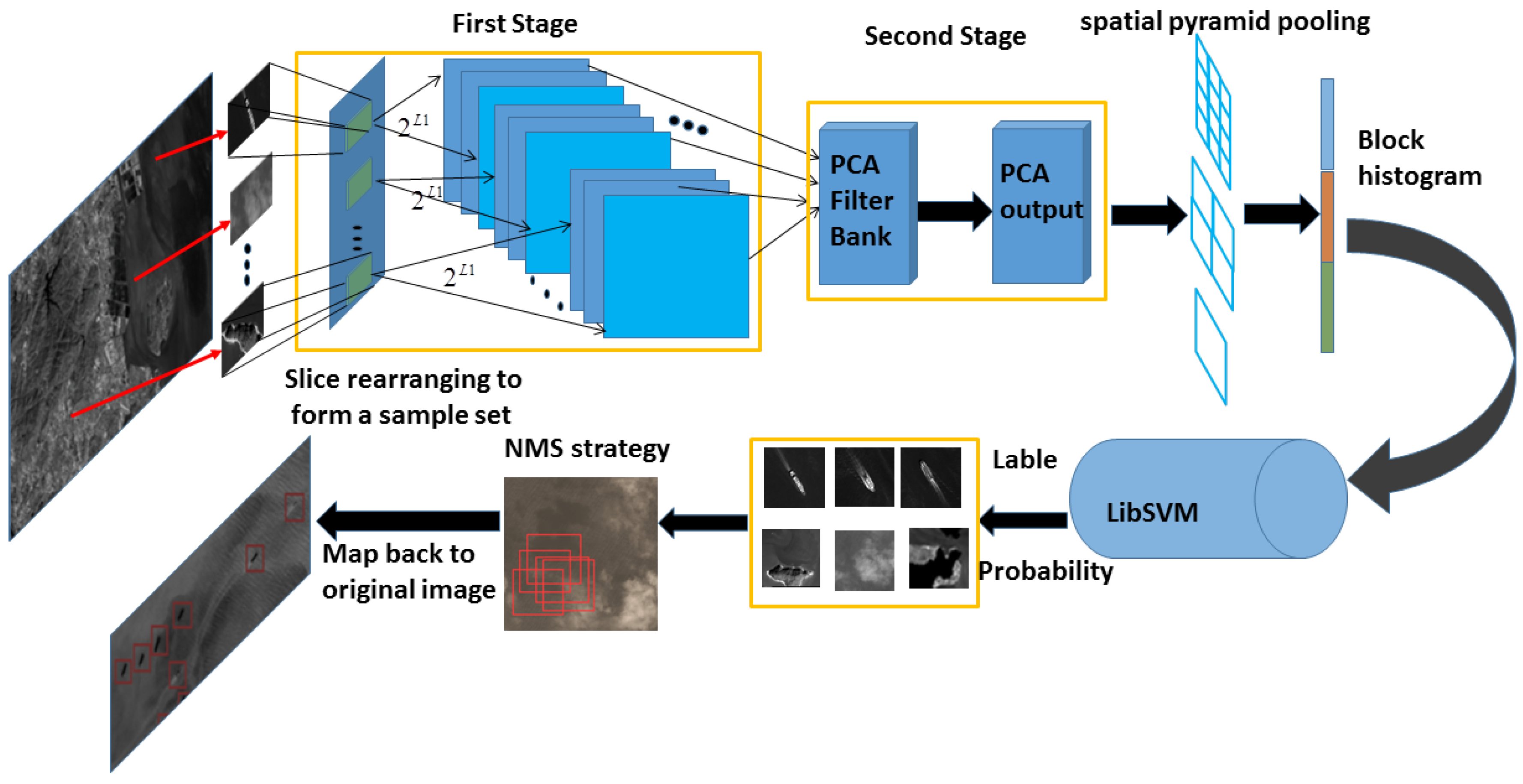
PCANet is a network model that is simpler in training process and can adapt to different tasks and different data types. PCANet mainly consists of three parts: (a) cascaded principal component analysis (PCA); (b) binary hash coding; and (c) block histogram. In this framework, a multi-layer filter kernel is first learned through the PCA method, and then binary hash coding and block histogram features are used for downsampling and encoding operations.
At this stage, feature extraction and classification are performed separately by PCANet and libSVM on the candidate slices obtained from the previous coarse detection. The features extracted by PCANet are used as input to the LibSVM to train the classifier. The fine detection phase further carefully identifies the candidate slice to eliminate the false alarm. Traditional methods for extracting features are Sift, HoG, LBP, Harr, etc. However, these features face great challenges for deformation, illumination, occlusion, background clutter, etc. In contrast, PCANet extracted features can make up for the shortcomings of traditional features, and its advantage is reflected in the more accurate classification of LibSVM, which can reduce more false positives and improve higher accuracy. The process of eliminating false alarms in the fine detection phase is shown in Figure 4.
Suppose there are N training pictures of size . In this experiment, each picture was drawn into a set of line vectors as a sample set, whose size is . We normalized the training image size to a size of 80 × 80. In addition, the number of filters in the first and second stages were 8 and 4, respectively, and the filter size was 7 × 7. In the first stage, principal component analysis was performed on N training pictures. Preprocessing, N training pictures can be obtained:
where is an image obtained after rearrangement and preprocessing of each image. In the first stage, the feature vector corresponding to the first largest feature values were extracted by solving the feature vector of as the filter of the next stage. The filter at this stage can be expressed as:
where denotes the fth principal eigenvector of . Then, the filters obtained in the first stage were, respectively, subjected to a convolution operation on the N images as an input of the second stage. Similar to the first stage, each obtained image was preprocessed, and the results of image segmentation were merged together.
where represents the block result of N pictures and one of the filter convolutions. Similarly, by solving the eigenvector of , the feature vector corresponding to the first L2 largest eigenvalues was taken as a filter.
The above formula represents the filter of the second stage. Then, through the spatial pyramid pooling, hash coding and histogram statistics, the feature vector of each training image was obtained. Finally, we inputed the trained feature vectors into the LibSVM to train and test them.
Generally, training with images of various sizes can improve scale invariance and reduce the occurrence of over fitting. This method adds spatial pyramid pooling (SPP) at the output layer of PCANet so that the input images can be trained by different sizes to generate a fixed-size output. Adding SPP to PCANet not only achieves the effect of multi-stage and multi-scale training, but also can extract and re-aggregate feature maps from different aspects. After each training was completed, the parameters of the network were reserved in the experiment. Then, another dimension was resized and the model based on the previous weight was retrained. Through experimental comparison, it was found that adding SPP can reduce the rate of missed detection, but within the allowable range, the false alarm rate was relatively increased.
In the experiment, we employed the non-maximum suppression (NMS) strategy to eliminate redundant overlapping frames, which can greatly reduce the false alarm rate. More than anything, PCANet has the following unique advantages compared with CNN. (a) The network structure for extracting features is simple. Each layer only performs PCA mapping, and binary hash coding and merging the process of histogram are carried out at the output of last layer. (b) A high level of experience and adjustment skill are not required. (c) The training and testing speed is faster than that of CNN. The CNN structure used in the experiment is as follows: Convolution → Pooling → Convolution → Pooling → Convolution → Pooling → Convolution → Pooling → Convolution → Dropout → Convolution → Softmax → Loss. In addition, the features extracted by PCANet are more efficient and do not excessively eliminate target candidate areas in the previous stage, increasing the detection rate and producing fewer false alarms than CNN.
3. Experimental Results and Analysis
3.1. Dataset Description
The sample data of the optical remote sensing image were derived from the GF-1 and GF-2 satellites. The experiment validated the proposed method on the GF-1 images of 18,192 × 18,000 pixels and GF2 images of 29,200 × 27,620 pixels. These datasets contain a variety of scenarios, such as cloud interference, low contrast, complex sea conditions, port vessels and so on. Before sending data to PCAnet training, we performed different data enhancements to improve performance. The data enhancements used include rotation, scaling, translation, left and right flipping and other operations. We collected 16,178 training samples (of which the validation set accounted for 3178) and 5394 test samples. There were 8343 positive samples and 7835 negative samples in the training set, while the numbers of positive and negative samples in the testing set were 2781 and 2613, respectively. The samples were reshaped to 80 × 80 pixels and stretched to 1 × 6401 as input to the PCANet model for training to extract features, with the last column being the sample label. The features extracted by the model were processed by SPP and then sent to the LibSVM classifier for training and classification. The display of positive and negative samples are shown in Figure 5.
3.2. Contrastive Experiments
To better evaluate the performance of the proposed algorithm in remote sensing image of different scenes, this work applied autocorrelation function to reflect the roughness of texture features [46,47] in a variety of situations. It can be used to measure the background complexity in different scenarios. In remote sensing image processing and interpretation, a multitude of feature are similar in shape, size and tone except for textures. The texture features of an image are often periodic, reflecting the texture of the image itself, such as roughness, smoothness, granularity, randomness, and normativeness. Texture analysis refers to the process of extracting texture features by certain image processing techniques to obtain quantitative or qualitative descriptions of textures. Autocorrelation function methods were employed in this study to extract texture features, which used as a texture measure to effectively reflect the roughness of texture images. Assuming the image is defined as , the autocorrelation function is:
where represents the offset value, and represents the displacement vector. The above equation shows that the autocorrelation function varies with the , which has a corresponding relationship with the change of the texture thickness in the image. More specifically, the algorithm calculates the correlation value between each pixel in the window and the offset value . Generally, the coarse texture region has a higher correlation for a given deviation () than the fine texture region, and thus the texture roughness should be proportional to the expansion of the autocorrelation function.
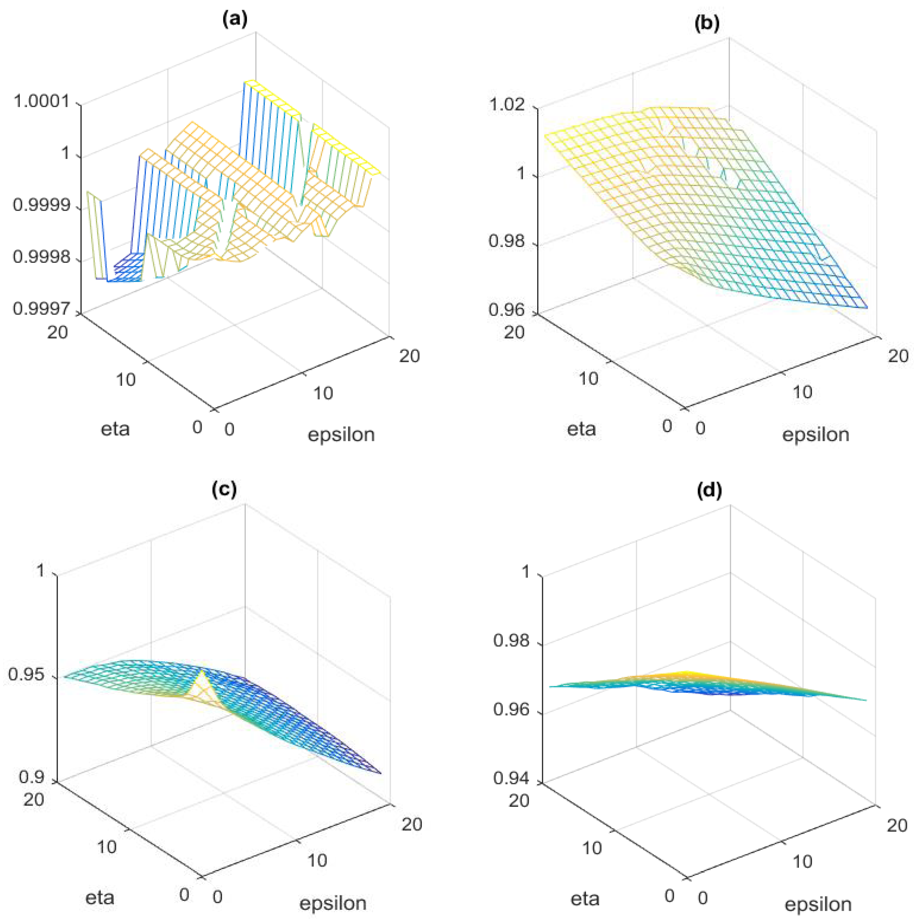
The texture of the image can reflect the roughness of the sea surface. In this experiment, the autocorrelation function is used as the texture measure, which reflects its roughness. Figure 6 reflects the complexity of the sea conditions under four different sea backgrounds: cloud cover, low contrast, complex surface waves and near the coast.
(a) Anomaly detection to extract target candidate regions
To verify the performance of our algorithm, we conducted a comparative analysis with different methods. For the selection of different sizes of the sliding window for anomaly detection, we chose the size of sliding windows as 5 × 5 in Reference [40]. In Reference [40], the size of 3 × 3, 5 × 5 and 9 × 9 sliding windows are experimentally validated, and the influence of experimental results is explained in detail. It is worth mentioning that the detection performance is optimal when the sliding window is chosen as 5 × 5. Figure 7 illustrates the comparison of the anomaly detection algorithm based on the multivariate Gaussian distribution with other candidate region extraction algorithms, including Otsu threshold segmentation and iterative threshold segmentation. It can be seen from experiments that, compared with other methods, our algorithm could excellently highlight the obvious ship area in the case of thin cloud cover (the red rectangle mark in the first row and the fourth column in Figure 7), large wave complex background and low contrast ship (the red rectangular marker in the third row and fourth column in Figure 7). Contrarily, the Otsu threshold segmentation has poor anti-interference ability to thin clouds and mist, and the abnormal regions caused by these false alarms will cover the area of the ship, causing missed detection. In the case of complex background of sea, Otsu threshold segmentation and iterative threshold segmentation led to more obvious segmentation of the ship and wake, resulting in too many connected domains (as shown in the red rectangular box markers in the second and third columns of the second row in Figure 7), which caused more false alarms. On the other hand, these two methods caused missed detection for ships with low contrast. Although adjusting threshold could reduce some false alarm interference, it also reduced the area of ship pixels, thus reducing the detection rate of ship targets. Compared with Otsu threshold segmentation and iterative threshold segmentation algorithms, the anomaly detection algorithm based on multivariate Gaussian distribution in this paper compensated for the defects of these two threshold segmentation methods. The experimental evaluation proved this assertion and showed that our approach effectively dealt with the limitations of the above two methods, especially in achieving significant improvements in some challenging images. The advantages of our approach are mainly reflected in the following facets: (a) the shape of the ship can retain a good anomalous area with fewer noise points; (b) it has better anti-interference for the background of complex sea conditions (such as large waves, thin clouds, mist, etc.); and (c) for vessels under thin cloud cover, it can be detected better.
(b) Fine detection to eliminate false alarms
For the GF1 image with a resolution of 2 m and the GF2 image with a resolution of 0.8 m, the length of the ship’s size ranged from about 30 m to 400 m in this experiment. Our experimental results were based on the statistics of ships whose number of pixels is more than 40. A ship with length less than 30 m is not within the statistical range. During the experiment, when the original image was directly input, and in the case where the SPP was not added, some missed detections occurred. Conversely, when SPP was added, the rate of missed detections was reduced, but the false alarm rate inevitably increased. In view of this, when the original image (18,192 × 18,000 pixels and 29,200 × 27,620 pixels) was cropped into multiple 1000 × 1000 size slices as input, the generated false alarms were basically overlapping boxes when the SPP was added. In light of this result, a non-maximum suppression strategy was utilized to exclude redundant boxes. This operation eliminated more false alarms, thus reducing the excess false rate. To better verify the effectiveness of the proposed method, the experiment were carried out, respectively, on clouds with low-interference, vessels with low contrast, complex sea-surface background and offshore conditions. The experimental results in these four scenarios are shown in Figure 8. Through experiments, we found that the method proposed in this paper can achieve a pleasurable detection effect. To verify the effectiveness of our work, the detection results were measured according to the four criteria of precision (P), recall (R), missed detection rate (MR) and false alarm rate (FR).
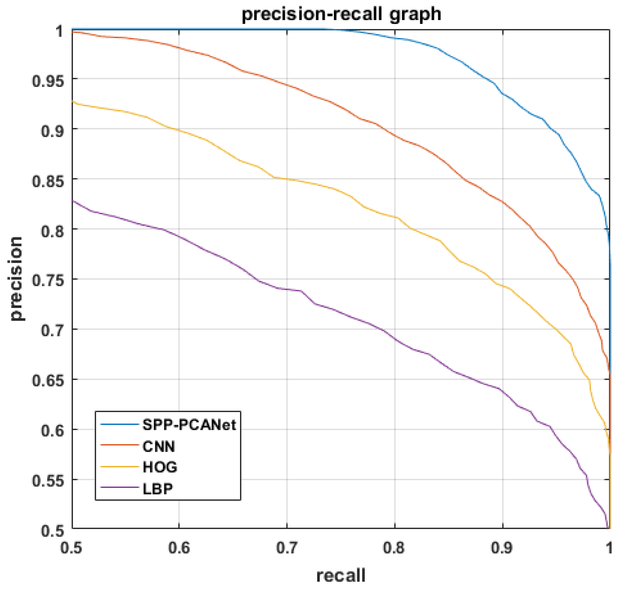
where represents the number of ships that are correctly detected and and are the total number of detections and the number of ships in the test dataset, respectively. We conducted comparative analysis of experiments with three kinds of feature extractor methods. Compared with the CNN, Hog and LBP features, the precision and recall rate of the experimental results of these methods are shown in the following. For detailed extraction and experimental results of each phase, Figure 9 and Table 1 give some reflections of the algorithm’s performance in terms of detection.
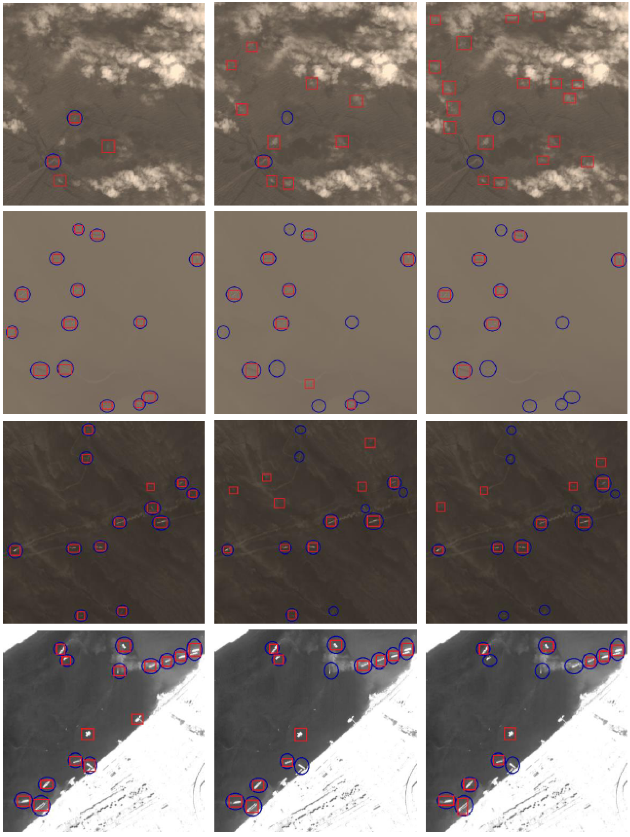
From the tabulate data, it is obvious that the algorithm proposed in this paper can achieve better detection performance. Most of the ship targets could be detected well, and the false alarm was maintained at around 15%. The recall rates of CNN, HOG and LBP are 0.84%, 0.73% and 0.64%, respectively. The recall rate of the ship detection algorithm proposed in this paper could reach 97%, which exceeds the other three methods. However, due to the addition of the spatial pyramid pooling operation, the false alarm rate of this method was higher than that of HOG algorithm, but lower than that of CNN and LBP. When strong interference exists, such as ships with relatively complex sea-surface background, low contrast, cloud interference, etc., the other three methods presented missed detections and excessive false alarms. This is because there are many scattered false alarms in the saliency map when selecting candidate regions. In particular, these feature extractors could not classify these false alarms and ship targets effectively, which led to the detection performance degradation. In Figure 10, the blue oval frame represents the ship target existing in the original image, and the red rectangular frame shows the detection result of different methods. It can be seen from the experimental comparison that, in the above four cases, the CNN, HOG and LBP features were less robust to cloud interference, ships with complex sea conditions, low contrast vessels, and near-shore vessels, which may cause missed detection. Conversely, our method showed favorable detection performance in face of the above situations.
4. Conclusions and Future Work
This study proposes a method for ship detection in optical remote sensing images by combining anomaly detection and spatial pyramid pooling of PCANet algorithms. First, the method adopts the sea–land segmentation strategy to overcome the difficulty of detecting the ships close to land, therefore reducing the large number of false alarms. Then, the anomaly detection algorithm is used to extract the candidate areas of the ships. Finally, within the scope of the false alarms, our method further improves the detection rate by joining SPP-PCANet with the concept of non-maximum suppression. A comparison with three algorithms, namely LBP, HOG and CNN, verifies that our method can achieve a high recall rate and reduce the rate of missed detections. In conclusion, the method developed in this study can achieve considerable robustness and effectiveness in the case of false alarm disturbances such as low contrast ships, ships with complex backgrounds, clouds and mists, and reefs.
Although our algorithm obtains desirable test results, some important problems still need to be solved. First, we will identify the types of ships in optical remote sensing images with high resolution so that the algorithm proposed here will find wider applications in military and civilian fields. In addition, to alleviate the difficulty in obtaining the sample of warships, we will integrate the concept of transfer learning into the algorithm and employ a large number of civilian ship samples to assist the detection of warship targets. Finally, we will create a target dataset with a manually labeled ground truth to better evaluate the performance of our proposed ship detection method.
Author Contributions
Conceptualization, B.L.; Methodology, N.W.; Validation, N.W.; Formal Analysis, N.W., Q.X. and Y.W.; Writing—Original Draft Preparation, N.W., Q.X. and Y.W.; and Writing—Review and Editing, N.W., B.L. and Q.X.
Funding
This research was funded by the National Natural Science Foundation of China (grant Nos. 61672076 and 61331017) and in part by the Army Equipment Research Project under grant 301020203.
Acknowledgments
The authors sincerely thank T. H. Chan, K. Jia and S. H. Gao for sharing their code. The authors also thank the assistant editor and the anonymous commentators for their insightful comments and suggestions. These suggestions have greatly improved the quality of this article.
Conflicts of Interest
The authors declare no conflict of interest.
References
- Tello, M.; Lopez-Martinez, C.; Mallorqui, J. A Novel Algorithm for Ship Detection in SAR Imagery Based on the Wavelet Transform. IEEE Geosci. Remote Sens. Lett. 2005, 2, 201–205. [Google Scholar] [CrossRef] [Green Version]
- Kang, M.; Ji, K.; Leng, X.; Lin, Z. Contextual region-based convolutional neural network with multilayer fusion for SAR ship detection. Remote Sens. 2017, 9. [Google Scholar]
- Leng, X.; Ji, K.; Zhou, S.; Xing, X.; Zou, H. An Adaptive Ship Detection Scheme for Spaceborne SAR Imagery. Sensors 2016, 16, 1345. [Google Scholar] [CrossRef] [PubMed]
- Benedek, C.; Descombes, X.; Zerubia, J. Building Development Monitoring in Multitemporal Remotely Sensed Image Pairs with Stochastic Birth-Death Dynamics. IEEE Trans. Pattern Anal. Mach. Intell. 2011, 34, 33–50. [Google Scholar] [CrossRef] [PubMed]
- Grinias, I.; Panagiotakis, C.; Tziritas, G. MRF-based segmentation and unsupervised classification for building and road detection in peri-urban areas of high-resolution satellite images. Isprs J. Photogram. Remote Sens. 2016, 122, 145–166. [Google Scholar] [CrossRef]
- Yang, X.; Sun, H.; Sun, X.; Yan, M.; Guo, Z.; Fu, K. Position Detection and Direction Prediction for Arbitrary-Oriented Ships via Multiscale Rotation Region Convolutional Neural Network. IEEE Access 2018, 6, 50839–50849. [Google Scholar] [CrossRef]
- Girshick, R.; Donahue, J.; Darrell, T.; Malik, J. Region-based Convolutional Networks for Accurate Object Detection and Segmentation. IEEE Trans. Pattern Anal. Mach. Intell. 2016, 38, 142–158. [Google Scholar] [CrossRef] [PubMed]
- Girshick, R.B. Fast R-CNN. In Proceedings of the International Conference on Computer Vision, Las Condes, Chile, 11–18 December 2015; pp. 1440–1448. [Google Scholar]
- Ren, S.; He, K.; Girshick, R.; Sun, J. Faster R-CNN: towards real-time object detection with region proposal networks. In Proceedings of the International Conference on Neural Information Processing Systems, Montreal, QC, Canada, 7–12 December 2015; pp. 91–99. [Google Scholar]
- Dai, J.; Li, Y.; He, K.; Sun, J. R-FCN: Object Detection via Region-based Fully Convolutional Networks. Neural Inf. Process. Syst. 2016, 379–387. [Google Scholar]
- Redmon, J.; Divvala, S.; Girshick, R.; Farhadi, A. You Only Look Once: Unified, Real-Time Object Detection. In Proceedings of the Computer Vision and Pattern Recognition, Las Vegas Valley, NV, USA, 26 June–1 July 2016; pp. 779–788. [Google Scholar]
- Liu, W.; Anguelov, D.; Erhan, D.; Szegedy, C.; Reed, S.; Fu, C.Y.; Berg, A.C. SSD: Single Shot MultiBox Detector. In Proceedings of the European Conference on Computer Vision, Amsterdam, The Netherlands, 8–16 October 2016; pp. 21–37. [Google Scholar]
- Lin, T.Y.; Dollar, P.; Girshick, R.; He, K.; Hariharan, B.; Belongie, S. Feature Pyramid Networks for Object Detection. In Proceedings of the IEEE Conference on Computer Vision and Pattern Recognition, Honolulu, HI, USA, 21–26 July 2017; pp. 936–944. [Google Scholar]
- He, K.; Gkioxari, G.; Dollar, P.; Girshick, R. Mask R-CNN. In Proceedings of the IEEE International Conference on Computer Vision, Venice, Italy, 22–29 October 2017; pp. 2980–2988. [Google Scholar]
- Lin, T.Y.; Goyal, P.; Girshick, R.; He, K.; Dollar, P. Focal Loss for Dense Object Detection. IEEE Trans. Pattern Anal. Mach. Intell. 2017, PP, 2999–3007. [Google Scholar]
- Kang, M.; Leng, X.; Lin, Z.; Ji, K. A modified faster R-CNN based on CFAR algorithm for SAR ship detection. In Proceedings of the International Workshop on Remote Sensing with Intelligent Processing, Shanghai, China, 19–21 May 2017; pp. 1–4. [Google Scholar]
- Yang, X.; Sun, H.; Fu, K.; Yang, J.; Sun, X.; Yan, M.; Guo, Z. Automatic Ship Detection of Remote Sensing Images from Google Earth in Complex Scenes Based on Multi-Scale Rotation Dense Feature Pyramid Networks. Remote Sens. 2018, 10, 132. [Google Scholar] [CrossRef]
- Lin, H.; Shi, Z.; Zou, Z. Maritime Semantic Labeling of Optical Remote Sensing Images with Multi-Scale Fully Convolutional Network. Remote Sens. 2017, 9, 480. [Google Scholar] [CrossRef]
- Qiu, S.; Wen, G.; Liu, J.; Deng, Z.; Fan, Y. Unified Partial Configuration Model Framework for Fast Partially Occluded Object Detection in High-Resolution Remote Sensing Images. Remote Sens. 2018, 10, 464. [Google Scholar] [CrossRef]
- Dong, C.; Liu, J.; Xu, F. Ship Detection in Optical Remote Sensing Images Based on Saliency and a Rotation-Invariant Descriptor. Remote Sens. 2018, 10, 400. [Google Scholar] [CrossRef]
- Xu, F.; Liu, J.; Dong, C.; Wang, X. Ship Detection in Optical Remote Sensing Images Based on Wavelet Transform and Multi-Level False Alarm Identification. Remote Sens. 2017, 9, 985. [Google Scholar] [CrossRef]
- Xu, F.; Liu, J.; Sun, M.; Zeng, D.; Wang, X. A Hierarchical Maritime Target Detection Method for Optical Remote Sensing Imagery. Remote Sens. 2017, 9, 280. [Google Scholar] [CrossRef]
- Proia, N.; Page, V. Characterization of a Bayesian Ship Detection Method in Optical Satellite Images. IEEE Geosci. Remote Sens. Lett. 2010, 7, 226–230. [Google Scholar] [CrossRef]
- Tang, J.; Deng, C.; Huang, G.B.; Zhao, B. Compressed-Domain Ship Detection on Spaceborne Optical Image Using Deep Neural Network and Extreme Learning Machine. IEEE Trans. Geosci. Remote Sens. 2014, 53, 1174–1185. [Google Scholar] [CrossRef]
- Zou, Z.; Shi, Z. Ship Detection in Spaceborne Optical Image With SVD Networks. IEEE Trans. Geosci. Remote Sens. 2016, 54, 5832–5845. [Google Scholar] [CrossRef]
- Li, Z.; Yang, D.; Chen, Z. Multi-layer Sparse Coding Based Ship Detection for Remote Sensing Images. In Proceedings of the IEEE International Conference on Information Reuse and Integration, Francisco, CA, USA, 13–15 August 2015; pp. 122–125. [Google Scholar]
- Li, H.; Li, Z.; Chen, Z.; Yang, D. Multi-layer sparse coding model-based ship detection for optical remote-sensing images. Int. J. Remote Sens. 2017, 38, 6281–6297. [Google Scholar] [CrossRef]
- Han, J.; Zhou, P.; Zhang, D.; Cheng, G.; Guo, L.; Liu, Z.; Bu, S.; Wu, J. Efficient, simultaneous detection of multi-class geospatial targets based on visual saliency modeling and discriminative learning of sparse coding. Isprs J. Photogram. Remote Sens. 2014, 89, 37–48. [Google Scholar] [CrossRef]
- Yokoya, N.; Iwasaki, A. Object Detection Based on Sparse Representation and Hough Voting for Optical Remote Sensing Imagery. IEEE J. Sel. Top. Appl. Earth Observ. Remote Sens. 2015, 8, 2053–2062. [Google Scholar] [CrossRef]
- Wang, X.; Shen, S.; Ning, C.; Huang, F.; Gao, H. Multi-class remote sensing object recognition based on discriminative sparse representation. Appl. Opt. 2016, 55, 1381–1394. [Google Scholar] [CrossRef] [PubMed]
- Wang, H.; Zhu, M.; Lin, C.; Chen, D. Ship detection in optical remote sensing image based on visual saliency and AdaBoost classifier. Optoelectron. Lett. 2017, 13, 151–155. [Google Scholar] [CrossRef]
- Qin, Y.; Lu, H.; Xu, Y.; Wang, H. Saliency detection via Cellular Automata. In Proceedings of the 2015 IEEE Conference on Computer Vision and Pattern Recognition (CVPR), Boston, MA, USA, 7–12 June 2015; pp. 110–119. [Google Scholar]
- Ao, W.; Xu, F.; Li, Y.; Wang, H. Detection and Discrimination of Ship Targets in Complex Background From Spaceborne ALOS-2 SAR Images. IEEE J. Sel. Top. Appl. Earth Observ. Remote Sens. 2018, 11, 536–550. [Google Scholar] [CrossRef]
- Nie, T.; He, B.; Bi, G.; Zhang, Y.; Wang, W. A Method of Ship Detection under Complex Background. ISPRS Int. J. Geo-Inf. 2017, 6, 159. [Google Scholar] [CrossRef]
- Song, Z.; Sui, H.; Wang, Y. Automatic ship detection for optical satellite images based on visual attention model and LBP. In Proceedings of the 2014 IEEE Workshop on Electronics, Computer and Applications, Lake Placid, NY, USA, 10 March 2014; pp. 722–725. [Google Scholar]
- Yang, F.; Xu, Q.; Gao, F.; Hu, L. Ship detection from optical satellite images based on visual search mechanism. In Proceedings of the Geoscience and Remote Sensing Symposium, Milan, Italy, 26–31 July 2015; pp. 3679–3682. [Google Scholar]
- Zhu, C.; Zhou, H.; Wang, R.; Guo, J. A Novel Hierarchical Method of Ship Detection from Spaceborne Optical Image Based on Shape and Texture Features. IEEE Trans. Geosci. Remote Sens. 2010, 48, 3446–3456. [Google Scholar] [CrossRef]
- Xia, Y.; Wan, S.; Yue, L. A Novel Algorithm for Ship Detection Based on Dynamic Fusion Model of Multi-feature and Support Vector Machine. In Proceedings of the International Conference on Image & Graphics, Hefei, China, 12–15 August 2011; pp. 521–526. [Google Scholar]
- Selvi, M.U.; Kumar, S.S. Sea Object Detection Using Shape and Hybrid Color Texture Classification. Commun. Comput. Inf. Sci. 2011, 204, 19–31. [Google Scholar]
- Shi, Z.; Yu, X.; Jiang, Z.; Li, B. Ship Detection in High-Resolution Optical Imagery Based on Anomaly Detector and Local Shape Feature. IEEE Trans. Geosci. Remote Sens. 2014, 52, 4511–4523. [Google Scholar]
- Li, Y.; Sun, X.; Wang, H.; Sun, H.; Li, X. Automatic Target Detection in High-Resolution Remote Sensing Images Using a Contour-Based Spatial Model. IEEE Geosci. Remote Sens. Lett. 2012, 9, 886–890. [Google Scholar] [CrossRef]
- Bi, F.; Zhu, B.; Gao, L.; Bian, M. A Visual Search Inspired Computational Model for Ship Detection in Optical Satellite Images. IEEE Geosci. Remote Sens. Lett. 2012, 9, 749–753. [Google Scholar]
- Zhu, J.; Qiu, Y.; Zhang, R.; Huang, J.; Zhang, W. Top-Down Saliency Detection via Contextual Pooling. J. Signal Process. Syst. 2014, 74, 33–46. [Google Scholar] [CrossRef]
- ElDarymli, K.; McGuire, P.; Power, D.; Moloney, C.R. Target detection in synthetic aperture radar imagery: A state-of-the-art survey. J. Appl. Remote Sens. 2013, 7, 071598. [Google Scholar] [CrossRef]
- Greidanus, H.; Kourti, N. Findings of the DECLIMS project—Detection and Classification of Marine Traffic from Space. In Proceedings of the Advances in SAR Oceanography from Envisat and ERS Missions, Frascati, Italy, 23–26 January 2006. [Google Scholar]
- Zheng, N.; Zheng, W.; Xu, Z.L.; Wang, D.C. Bridge Target Detection in SAR Images Based on Texture Feature. Appl. Mech. Mater. 2013, 347-350, 3634–3638. [Google Scholar] [CrossRef]
- Zhan, Y.; You, H.E. Fast Algorithm for Maneuvering Target Detection in SAR Imagery Based on Gridding and Fusion of Texture Features. Geo-Spat. Inf. Sci. 2011, 14, 169–176. [Google Scholar]
Figure 1.
The overall flow chart of target detection. The process from left to right are sea–land segmentation, candidate area extraction, false alarm exclusion, and detection results.
Figure 1.
The overall flow chart of target detection. The process from left to right are sea–land segmentation, candidate area extraction, false alarm exclusion, and detection results.

Figure 2.
The original images are in the first row of the figure, and the results of sea and land segmentation are the second row. Among them, the black area represent the land portions.
Figure 2.
The original images are in the first row of the figure, and the results of sea and land segmentation are the second row. Among them, the black area represent the land portions.

Figure 3.
Extraction of candidate regions of ship targets based on anomaly detection algorithm.

Figure 4.
Exclude false alarm diagram. PCANet feature extraction and LibSVM classifier flow chart.

Figure 5.
The presentation of positive and negative sample datasets. Among them, the scenes of positive samples in the first three columns are cloud interference, low contrast, and complex sea conditions; Columns 4–6 are positive samples in the normal sea background; and the last two columns are negative samples.

Figure 6.
Texture roughness under different background. Among them, (a–d) represent the background of low contrast, the port scene, complex sea surface, and cloud interference.
Figure 6.
Texture roughness under different background. Among them, (a–d) represent the background of low contrast, the port scene, complex sea surface, and cloud interference.

Figure 7.
The upper, middle, and lower rows are the results of abnormal detection of cloud (or mist) coverage, relatively complicated sea conditions, and low contrast of the ship. The first three columns from left to right represent the original image, iterative segmentation, and Otsu threshold segmentation, respectively, and the last column represents the anomaly detection results of the multivariate Gaussian distribution used in this paper.

Figure 8.
Target detection results of different methods under different experimental conditions: (a) cloud interference; (b) ship with low contrast; (c) complex sea conditions; and (d) near-shore vessel.
Figure 8.
Target detection results of different methods under different experimental conditions: (a) cloud interference; (b) ship with low contrast; (c) complex sea conditions; and (d) near-shore vessel.

Figure 9.
Precision and recall curves of different algorithms.

Figure 10.
Comparison of target detection results in different methods under different scenarios. The first column is the result of our method, the second column is the result of CNN, and the third column is the result of HOG.
Figure 10.
Comparison of target detection results in different methods under different scenarios. The first column is the result of our method, the second column is the result of CNN, and the third column is the result of HOG.


Table 1.
Comparison of accuracy and recall of ships by different methods.
| Algorithm | P (%) | R (%) | MR (%) | FR (%) | C_s | S_s |
|---|---|---|---|---|---|---|
| CNN | 0.83 | 0.84 | 0.16 | 0.17 | 361 | 430 |
| Hog | 0.86 | 0.73 | 0.27 | 0.14 | 314 | 430 |
| LBP | 0.82 | 0.64 | 0.36 | 0.18 | 275 | 430 |
| Our method | 0.85 | 0.97 | 0.03 | 0.15 | 417 | 430 |
© 2018 by the authors. Licensee MDPI, Basel, Switzerland. This article is an open access article distributed under the terms and conditions of the Creative Commons Attribution (CC BY) license (http://creativecommons.org/licenses/by/4.0/).
Share and Cite
MDPI and ACS Style
Wang, N.; Li, B.; Xu, Q.; Wang, Y. Automatic Ship Detection in Optical Remote Sensing Images Based on Anomaly Detection and SPP-PCANet. Remote Sens. 2019, 11, 47. https://doi.org/10.3390/rs11010047
AMA Style
Wang N, Li B, Xu Q, Wang Y. Automatic Ship Detection in Optical Remote Sensing Images Based on Anomaly Detection and SPP-PCANet. Remote Sensing. 2019; 11(1):47. https://doi.org/10.3390/rs11010047
Chicago/Turabian StyleWang, Nan, Bo Li, Qizhi Xu, and Yonghua Wang. 2019. "Automatic Ship Detection in Optical Remote Sensing Images Based on Anomaly Detection and SPP-PCANet" Remote Sensing 11, no. 1: 47. https://doi.org/10.3390/rs11010047
Note that from the first issue of 2016, this journal uses article numbers instead of page numbers. See further details here.