Analysis on the Effects of SAR Imaging Parameters and Environmental Conditions on the Standard Deviation of the Co-Polarized Phase Difference Measured over Sea Surface

Abstract

This study aimed at analyzing the effect of Synthetic Aperture Radar (SAR) imaging parameters and environmental conditions on the standard deviation of the co-polarized phase difference (${\sigma }_{{\phi }_C}$) evaluated over sea surface. The latter was shown to be an important polarimetric parameter widely used for sea surface target monitoring purposes. A theoretical model, based on the tilted-Bragg scattering, is proposed to predict the behavior of ${\sigma }_{{\phi }_C}$ against incidence angle for different roughness conditions. Then, a comprehensive experimental analysis, based on the processing of L-, C- and X-band polarimetric SAR scenes collected over different test areas under low-to-moderate wind conditions and covering a broad range of incidence angle, was carried out to discuss the effects of sensor’s and environmental parameters on sea surface ${\sigma }_{{\phi }_C}$. Results show that SAR imaging parameters severely affect ${\sigma }_{{\phi }_C}$, while the impact of meteo-marine conditions, under low-to-moderate wind regime, is almost negligible. Those outcomes have significant relevance to support the design of effective and robust algorithms for marine and maritime applications based on ${\sigma }_{{\phi }_C}$, including the detection of metallic targets (ships and offshore infrastructures as oil/gas platforms, aquacultures, wind farms, etc.) and polluted areas.

1. Introduction

The preservation and sustainable management of ocean resources and ecosystems are mandatory goals according to several international strategies, policy programmes and technical reports as the 2030 Agenda, the Blue Growth European Union program and the United Nations report for sustainable development [1,2,3,4,5]. Within this context, remote sensing tools, due to their synoptic view and frequent revisit time, are of paramount importance for a broad range of applications including global weather predictions, storm and hurricane warnings, wave and current forecastings, coastal storm surges, ship routing, commercial fishing and climate change [6].

Microwave imaging of sea surface from space allows the retrieval of several geophysical parameters that, once tailored models are available, can be transformed into added-value products that include, among others, significant wave height from radar altimeters, wave spectrum from Synthetic Aperture Radars (SARs), sea surface wind field from scatterometers and sea surface temperature and salinity from radiometers [6]. Furthermore, additional information on ocean targets of interest such as sea ice extent, pollutants, metallic infrastructures, icebergs, ships, etc. can be derived.

When dealing with microwave active remote sensing of the oceans, the unprecedented benefits offered by SAR sensors operating in multi-polarization modes is unambiguously recognized for a wide range of marine and maritime applications, including coastline extraction [7,8,9], metallic target detection [10,11,12], sea pollution monitoring [13,14,15,16] and sea ice observation [17,18,19]. All the approaches share a similar physical rationale that relies on the exploitation of the different polarimetric properties that characterize the target of interest and the sea clutter. Nonetheless, the performance is significantly affected by the amount of scattering information available that, in turn, depends on [8,10,14,20,21]:

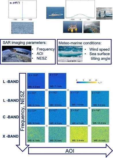
• SAR acquisition parameters, e.g., polarization, Angle Of Incidence (AOI), incident wavelength and Noise-equivalent sigma zero (NESZ);
• target features, e.g., damping properties of the pollutant, ship orientation and ice layer thickness; and
• meteo-marine conditions, e.g., sea state, swell and wave patterns.

Among the different polarimetric SAR architectures, conventional dual-polarimetric SAR imaging modes, i.e., the ones that consist of transmitting a linearly polarized wave (horizontal (H) or vertical (V)) while receiving coherently in an orthogonal linear basis (H–V), are attracting more attention in the perspective of operational services since they offer, for a wide range of ocean applications, a sufficient polarimetric information content over a large swath [7,16,22]. Among the dual-polarimetric SARs, it is worth mentioning the one operated by the German TerraSAR-X (TSX) mission that provides coherent HH-VV SAR measurements routinely. Among the polarimetric features that can be extracted from a coherent dual-polarimetric HH-VV SAR, the standard deviation of the co-polarized phase difference (${\sigma }_{{\phi }_C}$) has been demonstrated to be a powerful tool for marine and maritime applications. In fact, it is successfully used to perform the observation of metallic targets [23,24,25,26], the monitoring of oil pollution [14,16,27,28] and iceberg detection/sea ice classification [29,30].

All those applications share the same physical rationale, i.e., they exploit ${\sigma }_{{\phi }_C}$ as a reliable and robust estimator of the correlation between the co-polarized channels. This means that, at least from a theoretical viewpoint, since sea surface scattering is ruled by the Bragg mechanism, the co-polarized channels result in a unitary correlation that makes the co-polarized phase difference statistical distribution resembling a Dirac delta function [31,32,33,34]. In real cases, when a low-depolarizing scenario is considered, e.g., a sea surface Bragg scattering, a large correlation between co-polarized channels applies that results in a narrow co-polarized phase difference distribution. Hence, marine targets, e.g., ships, oil slicks, icebergs, etc., that result in departure from Bragg scattering are characterized by a broader co-polarized phase difference distribution. This means that ${\sigma }_{{\phi }_C}$ can be successfully exploited to emphasize non-Bragg scattering targets with respect to the Bragg-like sea surface background.

Following this rationale, in the literature, ${\sigma }_{{\phi }_C}$ has been mainly investigated in terms of sea/target separability (e.g., mean contrast and average target-to-clutter ratio are usually adopted as figures of merit [17,20,23,26,35]). In [28], ${\sigma }_{{\phi }_C}$ values spanning the range ≈ 3–18${}^{°}$ have been reported, at C-band, over sea surface under low-to-moderate wind conditions over different geographical locations. Dierking and Wesche [29] found that, at C-band, larger ${\sigma }_{{\phi }_C}$ values are in place when the measured co-polarized channels approach the sensor’s noise floor. In [30], ${\sigma }_{{\phi }_C}$ values of about 6${}^{°}$ have been measured at C-band with AOI = 40${}^{°}$ over sea surface and thin sea ice. In [10], larger ${\sigma }_{{\phi }_C}$ values, i.e., about 30${}^{°}$, have been measured over sea surface at X-band. The authors also observed a sensitivity of ${\sigma }_{{\phi }_C}$ with both the estimation window’s size and the sea state parameters. In [36], the behavior of ${\sigma }_{{\phi }_C}$ is investigated with reference to a specific test case, i.e., the Taylor Energy oil seep in the Gulf of Mexico, where a large TSX SAR dataset was considered under limited SAR imaging configuration (X-band, AOI = 26${}^{°}$, 34${}^{°}$ and 43${}^{°}$).

Hence, literature studies clearly point out the dependence of ${\sigma }_{{\phi }_C}$ on both sensor’s and environmental parameters. Nevertheless, the behavior of ${\sigma }_{{\phi }_C}$ is analyzed for specific applications only, i.e., for a given target (ships and oil slicks); sensor’s configuration, i.e., for a given frequency and/or limited AOI range; and environmental conditions [16,23,29,30,37]. In no case, to the best of our knowledge, the role of sensor’s and environmental parameters on ${\sigma }_{{\phi }_C}$ is investigated in a systematic way.

In this study, a significant extension of the work carried out in [36] was made. The analysis undertaken in [36] was improved as follows:

• The analysis on the effects of different frequencies, i.e., L- and C-band, and sea surface tilting angle on sea surface ${\sigma }_{{\phi }_C}$ was included.
• The analysis on the influence of incidence angle on sea surface ${\sigma }_{{\phi }_C}$ was undertaken on a much broader AOI range, i.e., about 20–60${}^{°}$.
• The behavior of sea surface ${\sigma }_{{\phi }_C}$ with respect to AOI was investigated by comparing model predictions’ with actual SAR measurements over the whole range of Bragg AOIs (≈20–60${}^{°}$).

Hence, a comprehensive analysis on the behavior of ${\sigma }_{{\phi }_C}$ over sea surface was provided for the first time. A large polarimetric SAR dataset collected in a wide range of SAR acquisition parameters (frequency, AOI, and NESZ) and meteo-marine conditions (sea surface roughness and wind speed (WS)) was considered to give a more complete understanding on how those parameters affect sea surface ${\sigma }_{{\phi }_C}$. Furthermore, to better interpret the experimental results, a theoretical scattering framework, based on the polarimetric X-Bragg model, is proposed that allows giving a physical understanding of the behavior of sea surface ${\sigma }_{{\phi }_C}$ under noise-free conditions. It must be explicitly pointed out that this comprehensive study is of paramount importance to support all the operational techniques based on ${\sigma }_{{\phi }_C}$, e.g., to find the most suitable SAR configuration in relation with the ocean target to be detected.

The remainder of the paper is organized as follows: in Section 2, the theoretical background that lies at the basis of the sensitivity analysis is presented; in Section 3, SAR dataset and ancillary information are provided; in Section 4, the experiments based on the theoretical model provided in Section 2 are presented and discussed; in Section 5, experiments related to the sensitivity analysis undertaken on the actual SAR dataset are presented and discussed; and conclusions are drawn in Section 6.

2. Polarimetric Framework

The co-polarized phase difference was theoretically predicted over sea surface using a polarimetric sea surface scattering model. The latter, based on the X-Bragg scattering model developed in [36], assumed that sea surface is mainly governed by the tilted-Bragg scattering mechanism. This is a reasonable assumption under low-to-moderate wind conditions (i.e., ≈ 2–14 m/s) and under intermediate AOIs (i.e., ≈ 20–60${}^{°}$).

From the scattering viewpoint, sea surface is considered as a distributed low-depolarizing scene. Hence, second-order descriptors, i.e., the covariance matrix $\mathbf{C}$, are needed to describe sea surface polarimetric scattering [38]. In the monostatic backscattering case, invoking reciprocity and the reflection symmetry property, the 3 × 3 Hermitian and semi-definite positive covariance matrix $\mathbf{C}$ can be defined as follows [38]:

$$\mathbf{C}=\left(\begin{array}{ccc}{C}_{11}& C_{12}& C_{13}\\ {C_{12}}^{*}& C_{22}& C_{23}\\ {C_{13}}^{*}& {C_{23}}^{*}& C_{33}\end{array}\right)=\left(\begin{array}{ccc}\langle |S_{hh}{|}^2\rangle & 0& \langle S_{hh}{S_{vv}}^{*}\rangle \\ 0& 2\langle |S_{hv}{|}^2\rangle & 0\\ \langle S_{vv}{S_{hh}}^{*}\rangle & 0& \langle |S_{vv}{|}^2\rangle \end{array}\right),$$

(1)

where $S_{pq}$ is the complex scattering amplitude with $\left\{p,q\right\}=\left\{h,v\right\}$, while $\langle ·\rangle$, $|·|$ and ${}^{*}$ stand for ensemble average, modulus and complex conjugate operators, respectively.

According to the X-Bragg scattering theory, the sea surface covariance matrix can be predicted as follows [39,40,41]:

$$\begin{array}{c}{\mathbf{C}}_{\mathbf{X}}=\left(\begin{array}{ccc}{C}_{X_{11}}& 0& C_{X_{13}}\\ 0& C_{X_{22}}& 0\\ {C_{X_{13}}}^{*}& 0& C_{X_{33}}\end{array}\right)=\\ {\mathbf{U}}^{-1}\left(\begin{array}{ccc}|B_h+B_v{|}^2& (B_h+B_v)({B_h}^{*}-{B_v}^{*})\mathrm{sinc}\left(2\beta \right)& 0\\ ({B_h}^{*}+{B_v}^{*})(B_h-B_v)\mathrm{sinc}\left(2\beta \right)& \frac{1}{2}{|B_h-B_v|}^2\left(1+\mathrm{sinc}\left(4\beta \right)\right)& 0\\ 0& 0& \frac{1}{2}{|B_h-B_v|}^2\left(1-sinc\left(4\beta \right)\right)\end{array}\right)\mathbf{U},\end{array}$$

(2)

where the subscript “X” stands for X-Bragg model and $\mathbf{U}$ is a con-similarity linear transformation given by [38]:

$$\mathbf{U}=\frac{1}{\sqrt{2}}\left(\begin{array}{ccc}1& 0& 1\\ 1& 0& -1\\ 0& \sqrt{2}& 0\end{array}\right).$$

(3)

In Equation (2), $\beta$ is the surface local tilting angle, while $B_h$ and $B_v$ are the Fresnel complex coefficients for Bragg scattering under horizontal and vertical polarizations, respectively, which are given by [41]:

$$\left\{\begin{array}{c}{B}_h=\frac{\cos (\mathrm{AOI})-\sqrt{ϵ-{\sin }^2(\mathrm{AOI})}}{\cos (\mathrm{AOI})+\sqrt{ϵ-{\sin }^2(\mathrm{AOI})}}\hfill \\ B_v=\frac{(ϵ-1)\left({\sin }^2(AOI)-ϵ\left(1+{\sin }^2(AOI)\right)\right)}{{\left(ϵ\cos (AOI)+\sqrt{ϵ-{\sin }^2(AOI)}\right)}^2}\hfill \end{array}\right..$$

(4)

In the X-Bragg sea surface scattering model, $\beta$ is related to the amount of surface roughness and it rules both the cross-polarized backscattering and the HH-VV coherence, while the Bragg scattering coefficients are related to the incidence angle and to the frequency-dependent relative electric permittivity of seawater, $ϵ$ [41]. $\beta$ was assumed to be uniformly distributed in the range [−90${}^{°}$, +90${}^{°}$], where $\beta$ ≈ 0${}^{°}$ describes an almost flat sea surface (negligible cross-polarized backscattering and HH-VV coherence close to 1), while $\beta$ ≈ ±90${}^{°}$ characterizes an extremely rough sea surface (significant cross-polarized backscattering and HH-VV coherence that tends to 0) [41]. In [15,40], it is found that reliable $\beta$ values fall within the range [−30${}^{°}$, 30${}^{°}$].

Once $\mathbf{C}$ is predicted according to the X-Bragg scattering model, the co-polarized phase difference can be obtained:

$$\angle C_{X_{13}}=\angle \left(\frac{1}{2}|B_h+B_v{|}^2-\frac{1}{4}{|B_h-B_v|}^2\left(1-\mathrm{sinc}(4\beta )\right)-j\Im ({B_h}^{*}+{B_v}^{*})(B_h-B_v)\mathrm{sinc}(2\beta )\right),$$

(5)

where $\angle (·)$ and $\Im (·)$ mean phase and imaginary part, respectively. Note that Equation (5) allows explicitly pointing out the relationship between the co-polarized phase difference and SAR acquisition parameters (through the Bragg scattering coefficients, i.e., AOI and frequency) and geometric/dielectric properties of sea surface (through $\beta$ and $ϵ$). Hence, it is a starting point to understand the effects of such parameters on the co-polarized phase difference distribution.

3. Datasets

In this section, the SAR dataset and the ancillary data are briefly described.

3.1. SAR Dataset

The L-, C- and X-band polarimetric SAR dataset consists of 14 scenes acquired between June 2006 and July 2013. The two L-band Single-look complex (SLC) full-polarimetric Uninhabited Aerial Vehicle Synthetic Aperture Radar (UAVSAR) scenes were acquired with an AOI ranging from about 22${}^{°}$ to 65${}^{°}$ in the northern part of the Gulf of Mexico. The UAVSAR system operates at center frequency of 1.26 GHz and is characterized by a NESZ of about −53 dB at mid-swath [42].

The four L-band SLC full-polarimetric ALOS PALSAR-1 (AP) scenes were acquired between June 2006 and April 2009 with an AOI from about 22${}^{°}$ to 25${}^{°}$ in the northern part of the Gulf of Mexico and off the northeastern coast of Brazil. The Japanese AP system operates at center frequency of 1.27 GHz with a NESZ of −29 dB at near range (21.5${}^{°}$) [43].

The four C-band SLC full-polarimetric RADARSAT-2 (RS) scenes were collected between January 2009 and May 2010 with AOI ranging from about 22${}^{°}$ to 41${}^{°}$ in the northern part of the Gulf of Mexico and off the California coast. The Canadian RS system operates at center frequency of 5.40 GHz with a NESZ of −35 dB [44].

The four X-band SLC dual co-polarimetric HH-VV TSX scenes were collected between December 2011 and July 2012 with an AOI range of 25${}^{°}$ to about 35${}^{°}$ in the northern part of the Gulf of Mexico. The German TSX system operates at center frequency of 9.60 GHz with a mean NESZ of −22 dB [45].

Figure 1 shows excerpts (1000 × 1000 pixels) of the VV-polarized intensity images of the whole SAR dataset representing homogeneous sea surface areas. Figure 1 is organized in a matrix format, where rows refer to the different SAR sensors (UAVSAR, AP, RS and TSX from the top to the bottom) and columns are arranged according to increasing AOI (from left to right). Note that, even though the same decibel (dB) scale is adopted, i.e., [0 −40], the sea surface patterns and, therefore, the backscattering change significantly according to the SAR imaging parameters and meteo-marine conditions. An overview of the SAR dataset is provided in

Table 1. General information on SAR imagery.

SAR Sensor	UAVSAR	AP	RS	TSX
Frequency (GHz)	1.26	1.27	5.40	9.60
Imaging mode	Full-polarimetric	Full-polarimetric	Full-polarimetric	Dual co-polarimetric
Slant range × azimuth resolution (m)	1.7 × 1.0	9.4 × 3.6	4.7 × 5.1	1.2 × 6.6
Number of scenes	2	4	4	4
Nominal NESZ (dB)	−53	−29	−35	−22

and

Table 2. Overview of the dataset.

SAR Data				Ancillary Wind Info
SAR Sensor	Scene ID	Acquisition Date	AOI Range (${}^{°}$)	Speed (m/s)	Direction (${}^{°}$)
UAVSAR	1	25/07/2013	22.0–27.0	4.2	115.4
			31.0–35.0
			38.0–42.0
	2	22/06/2010	22.0–26.0	7.1	321.0
			31.0–35.0
			38.0–42.0
AP	3	02/04/2009	22.7–25.0	3.1	232.0
	4	20/06/2006	22.7–25.0	4.9	298.6
	5	14/03/2007	22.7–25.0	7.4	332.2
	6	19/03/2009	22.7–25.0	8.0	243.3
RS	7	31/01/2009	22.6–24.2	9.0	215.1
	8	04/05/2010	23.4–25.3	4.3	129.3
	9	26/09/2009	31.3–33.0	4.7	142.9
	10	01/05/2010	39.3–40.7	12.0	331.3
TSX	11	01/07/2012	25.0–26.7	4.1	1.3
	12	05/12/2011	25.0–26.7	9.2	5.1
	13	17/05/2012	33.0–34.5	3.8	168.6
	14	19/06/2012	33.0–34.5	8.4	305.0

. Note that the whole SAR dataset is partitioned according to three AOI ranges: low (22–27${}^{°}$), intermediate (31–35${}^{°}$) and high (38–42${}^{°}$) (see Table 2).

3.2. Ancillary Wind Field Information

The wind information was provided by the Physical Oceanography Distributed Active Archive Center (PO.DAAC) that makes available science data to a wide user community [46,47,48]. The wind information was collected from two different sources depending on the SAR imagery acquisition period. The wind field co-located to SAR scenes acquired before 2012 was collected from the Cross-Calibrated Multi-Platform (CCMP) project, while the wind field related to the SAR scenes acquired since 2012 was collected from the Advanced Scatterometer (ASCAT) instrument on MetOp-A (Meteorological Operational Satellites) satellite.

The CCMP product is characterized by a spatial resolution of about 25 km and combines cross-calibrated satellite winds from RMS Remote Sensing Systems derived from microwave radiometers and from scatterometers, in situ measurements and reanalysis data from the European Center for Medium-Range Weather Forecasts (ECMWF) ERA-40 Reanalysis [49]. The wind products obtained from ASCAT are characterized by an effective resolution of 50 km and are delivered by the European Organization for the Exploitation of Meteorological Satellites (EUMETSAT) Ocean and Sea Ice Satellite Application Facility (OSI SAF) through the Royal Netherlands Meteorological Institute (KNMI) [50].

The SAR scenes were all collected under low-to-moderate wind conditions, i.e., from about 3 m/s to 12 m/s. The wind information is summarized in Table 2.

4. Model-Based Experimental Results

In this section, the behavior of ${\sigma }_{{\phi }_C}$ against AOI and $\beta$ is discussed using both the theoretical model presented in Section 2 and actual polarimetric SAR measurements collected by UAVSAR (see Table 1 and Table 2). The latter, on the one side, is characterized by a very low NESZ that guarantees high-quality measurements even at larger AOIs, while, on the other side, UAVSAR scenes cover a broad range of AOIs (spanning from about 20${}^{°}$ to 60${}^{°}$) and, therefore, they make possible comparing theoretical predictions with actual measurements over the whole range of Bragg AOIs.

To predict realistic ${\sigma }_{{\phi }_C}$ values, we used $\beta$ values estimated from the UAVSAR scenes using the formula proposed in [51]:

$$\mathrm{sinc}(4\beta )=\frac{Tr(\mathbf{C})-2C_{22}-0.5\Re (C_{13})}{Tr(\mathbf{C})-0.5\Re (C_{13})},$$

(6)

where $Tr(·)$ is the trace operator and $\Re (·)$ means real part. Hence, for each SAR scene, three equal-sized homogeneous sea surface regions of interest (ROIs) were excerpted that are characterized by low (22–27${}^{°}$), intermediate (31–35${}^{°}$) and high (38–42${}^{°}$) AOI, respectively. Accordingly, to better understand the behavior of $\beta$, normalized histograms were computed (see Figure 2). It can be noted that the empirical statistical distribution of $\beta$ (see blue histograms) resembles a Gaussian bell for any AOI, as witnessed by the fitted distribution (see red curves) that satisfies the chi-square test with 0.05 confidence interval.

Once $\beta$ was obtained, to predict ${\sigma }_{{\phi }_C}$, a Monte Carlo approach based on 1000 independent simulations for each AOI was implemented.

For each simulation, $\beta$ was randomly selected according to a Gaussian distribution whose mean and standard deviation values were obtained from the UAVSAR ROIs, i.e., 9.9${}^{°}$ and 0.8${}^{°}$ for the UAVSAR scene ID 1 and 7.3${}^{°}$ and 0.7${}^{°}$ for the UAVSAR scene ID 2 (see

Table 3. Values of ${\sigma }_{{\phi }_C}$, $\beta$ and HH and VV SNR evaluated within ROIs selected over a homogeneous sea surface area. ${\sigma }_{{\phi }_C}$ and $\beta$ are presented as mean ± standard deviation value.

SAR Sensor	ID	AOI (${}^{°}$)	${\mathit{\sigma }}_{{\mathit{\phi }}_{\mathit{C}}}$ (${}^{°}$)	WS (m/s)	$\mathit{\beta }$ (${}^{°}$)	SNR (dB)
						HH	VV
UAVSAR	1	22.0–27.0	1.0 ± 0.4	4.2	9.6 ± 0.8	39.0	38.7
		31.0–35.0	1.1 ± 0.5		10.2 ± 0.9	35.6	35.9
		38.0–42.0	1.4 ± 0.5		10.0 ± 0.7	30.1	32.1
	2	22.0–26.0	0.7 ± 0.3	7.1	6.6 ± 0.7	38	40.3
		31.0–35.0	1.0 ± 0.4		7.7 ± 0.7	35.7	38.7
		38.0–42.0	1.3 ± 0.5		7.5 ± 0.6	30.2	34.9
AP	3	22.7–25.0	3.0 ± 1.3	3.1	8.3 ± 2.0	18.7	20.3
	4	22.7–25.0	3.2 ± 1.3	4.9	8.2 ± 2.0	19.3	20.3
	5	22.7–25.0	3.2 ± 1.4	7.4	7.3 ± 1.7	21.2	22.0
	6	22.7–25.0	3.0 ± 1.2	8.0	9.5 ± 2.3	20.8	21.5
RS	7	22.6–24.2	4.0 ± 2.0	9.0	5.9 ± 1.7	27.8	28.2
	8	23.4–25.3	3.7 ± 1.7	4.3	6.7 ± 1.9	27.4	27.8
	9	31.3–33.0	5.0 ± 2.3	4.7	8.4 ± 2.6	19.2	21.4
	10	39.3–40.7	8.0 ± 4.0	12.0	9.6 ± 3.2	14.5	18.2
TSX	11	25.0–26.7	8.8 ± 6.4	4.1	–	9.2	9.8
	12	25.0–26.7	7.4 ± 5.7	9.2	–	10.2	10.4
	13	33.0–34.5	18.4 ± 16.5	3.8	–	2.7	3.8
	14	33.0–34.5	12.6 ± 10.0	8.4	–	5.8	7.9

).

Simulation results are depicted in Figure 3a, where the continuous and dashed lines are related to $\beta$ extracted from UAVSAR scenes ID 1 and ID 2, respectively. It can be noted that, in both cases, ${\sigma }_{{\phi }_C}$ increases with AOI, with ${\sigma }_{{\phi }_C}$ values ranging from about 0.01${}^{°}$ at near range to about 0.15${}^{°}$ at far range.

${\sigma }_{{\phi }_C}$ values measured from actual UAVSAR scenes using a 9 × 9 moving window are depicted in Figure 3b, where continuous and dashed lines stand for UAVSAR scene ID 1 and ID 2, respectively. It can be noted that both measured and simulated ${\sigma }_{{\phi }_C}$ increase with the incidence angle. This witnesses that the X-Bragg model succeeds in predicting the actual behavior of ${\sigma }_{{\phi }_C}$ with respect to AOI. However, the simulated and measured ${\sigma }_{{\phi }_C}$ values are completely different, i.e., the simulated ${\sigma }_{{\phi }_C}$ values are about one order of magnitude smaller (measured ${\sigma }_{{\phi }_C}$ values range from about 0.5${}^{°}$ at near range to about 4${}^{°}$ at far range). Nonetheless, this is not a surprising result. The theoretical scattering model predicts a noise-free behavior referred to a low-depolarizing Bragg scattering surface, i.e., the co-polarized phase difference distribution should resemble, ideally, a Dirac delta function (i.e., ${\sigma }_{{\phi }_C}=0^{°}$), while UAVSAR measurements, although very accurate, are noisy and refer to a real scattering surface, i.e., sensor and environmental parameters cause decorrelation between the co-polarized channels that results in a broader co-polarized phase difference distribution (i.e., larger ${\sigma }_{{\phi }_C}$ values). Note that a similar trend for ${\sigma }_{{\phi }_C}$ is experimentally observed in [42]. Notwithstanding that, the global ${\sigma }_{{\phi }_C}$ behavior with respect to AOI is well-described by the X-Bragg scattering model.

Figure 3 also shows that the model succeeds in predicting ${\sigma }_{{\phi }_C}$ values related to the UAVSAR scene ID 1, which are slightly larger than the corresponding ones related to the UAVSAR scene ID 2. This is because actual $\beta$ values were used in the simulations.

5. Experimental Results

The sensitivity of ${\sigma }_{{\phi }_C}$ with respect to acquisition parameters, i.e., AOI, NESZ and incident wavelength, and meteo-marine conditions, i.e., WS and $\beta$, was analyzed using actual polarimetric SAR data (Table 1 and Table 2). When dealing with SAR imaging parameters, hardware and technical constraints suggest that there is a close relationship among NESZ, AOI and wavelength [45,52]. In addition, from a scattering viewpoint, when a Bragg surface backscattering is considered, the larger is the AOI, the lower is the signal-to-noise ratio (SNR), i.e., the mean ratio between co-polarized sea surface backscattering and the nominal NESZ [36,42]. When dealing with meteo-marine parameters, both $\beta$ and near-surface wind speed are related to geometrical sea surface characteristics, i.e., sea surface roughness. Hence, a preliminary analysis devoted to understanding the relationship between $\beta$ and WS is due.

To accomplish this task, the normalized $\beta$ histograms were evaluated for each ROI belonging to AP and RS SAR scenes for low, intermediate and high AOIs (see Figure 4), where the mean WS values obtained from the external sources described in Section 3.2 were also annotated. First, it can be noted that $\beta$ normalized histograms are broader (about 2–3 times) than the corresponding UAVSAR ones (see Figure 2). This is most likely due to the higher NESZ that characterizes AP and RS rather than rougher sea state conditions (see Table 3). In addition, no clear relationship between WS and $\beta$ was observed. This suggests that, although both $\beta$ and WS are related to the sea surface roughness, there is no clear link between them. Consequently, the sensitivity of ${\sigma }_{{\phi }_C}$ with respect to WS and $\beta$ deserves to be analyzed separately.

Hence, the whole SAR dataset was processed according to the methodology described in Section 4 for the UAVSAR case. The only difference relies on the fact that AP, RS and TSX SAR scenes are characterized by a significantly narrower AOI range if compared to UAVSAR (less than 3${}^{°}$ from near to far range, see Table 2) and, therefore, only one ROI was selected for each scene. ${\sigma }_{{\phi }_C}$ maps, obtained according to Migliaccio et al. [28], are shown in Figure 5, where it can be noted how ${\sigma }_{{\phi }_C}$ is affected by both SAR imaging parameters and environmental conditions. In fact, ${\sigma }_{{\phi }_C}$ values range from about 0${}^{°}$ to more than 15${}^{°}$ along the whole dataset. The lowest ${\sigma }_{{\phi }_C}$ values are shown in Figure 5a,b, corresponding to UAVSAR acquisitions (L-band, NESZ = −53 dB), while the largest values are related to TSX acquisitions (X-band, NESZ = −22 dB) (see Figure 5m,n). In addition, since columns in Figure 5 are organized according to increasing AOI (as in Figure 1), it can be noted that ${\sigma }_{{\phi }_C}$ increases with AOIs, as suggested by the model-based analysis presented in Section 4.

The visual interpretation was confirmed by the quantitative analysis undertaken on 1000 independent samples, randomly selected from the ROIs, whose ${\sigma }_{{\phi }_C}$ mean and standard deviation values were evaluated together with the average SNR (see Table 3). In Table 3, mean and standard deviation values of the $\beta$ parameter estimated from the whole dataset according to Equation (6) are also listed. It must be noted that $\beta$ values related to TSX SAR scenes are not available since full-polarimetric information is needed to estimate $\beta$. The following subsections focus on the quantitative analysis of the effects produced by sensor and scene parameters on sea surface ${\sigma }_{{\phi }_C}$, separately.

5.1. Sensitivity Analysis: Meteo-Marine Parameters

The influence of WS and $\beta$ on ${\sigma }_{{\phi }_C}$ was analyzed. When dealing with the effects of WS on ${\sigma }_{{\phi }_C}$, according to Table 2, the AP SAR imagery were considered since the four SAR scenes were acquired under very similar SAR imaging parameters, i.e., the same AOI (≈24${}^{°}$) and incident wavelength (L-band), and by almost the same estimated mean SNR, i.e., ≈19–22 dB for both channels (see Table 3). Results listed in Table 3 clearly point out that, although the AP SAR scenes were collected under different wind conditions, i.e., ≈3 m/s and 8 m/s for SAR scene ID 3 and 6, respectively, they are characterized by very similar ${\sigma }_{{\phi }_C}$ mean values, i.e., ≈ 3.1${}^{°}$. In addition, WS does not affect significantly the variability of ${\sigma }_{{\phi }_C}$—see the standard deviation of ${\sigma }_{{\phi }_C}$ in Table 3, which is close to ≈ 1.3${}^{°}$ for all AP SAR scenes. The same comments apply for SAR scene ID 4 and 5. Hence, it can be concluded that, under low-to-moderate wind conditions, ${\sigma }_{{\phi }_C}$ is almost unaffected by WS.

To discuss the effects of $\beta$ on ${\sigma }_{{\phi }_C}$, it is worth analyzing results that refer to AP and RS SAR imagery—see ID 5–8 in Table 3, since they refer to SAR scenes collected under similar acquisition parameters, i.e., L-band, AOI of ≈ 24${}^{°}$ and average SNR of about 21 dB (C-band, AOI of ≈ 24${}^{°}$ and average SNR of about 28 dB). It can be noted that, from the results in Table 3, SAR scenes ID 5 and 6 are characterized by almost the same ${\sigma }_{{\phi }_C}$ values, i.e., 3.1${}^{°}$± 1.3${}^{°}$, although SAR scene ID 6 is characterized by a $\beta$ value that is about 30% larger than the one related to the SAR scene ID 5. The same comments apply for SAR scene ID 7 and 8, which are characterized by almost the same ${\sigma }_{{\phi }_C}$ values, i.e., 4.0${}^{°}$ ± 2.0${}^{°}$ and 3.7${}^{°}$± 1.7${}^{°}$, respectively, although the $\beta$ parameter estimated from SAR scene ID 7 is about 25% larger than the one evaluated from SAR scene ID 8.

Hence, this experimental analysis shows that there is no clear trend between $\beta$ and ${\sigma }_{{\phi }_C}$. In particular, $\beta$ does not play a dominant role in broadening/shrinking the co-polarized phase difference distribution.

5.2. Sensitivity Analysis: SAR Imaging Parameters

The influence of noise floor, incidence angle and wavelength on ${\sigma }_{{\phi }_C}$ was analyzed. As explicitly pointed out above, it is not straightforward to isolate their individual contribution since they are inter-connected.

To analyze the effects of NESZ on ${\sigma }_{{\phi }_C}$, SAR scenes collected by the L-band UAVSAR and AP platforms were considered since they are characterized by completely different NESZ values, i.e., −53 dB and −29 dB, respectively (see Table 1), while sharing the same operating frequency. In addition, the AOI range that characterizes AP SAR scenes was included into the one provided by UAVSAR. Hence, those datasets allow a fair analysis of the impact of noise floor in broadening/shrinking the co-polarized phase difference distribution. UAVSAR scenes ID 1 and ID 2 and AP SAR scenes ID 3–6 are characterized by a SNR equal to ≈39 dB and ≈21 dB, respectively (see Table 3). Their mean ${\sigma }_{{\phi }_C}$ values are 0.85${}^{°}$ and 3.1${}^{°}$, respectively. Hence, one can note that, when halving the SNR, ${\sigma }_{{\phi }_C}$ increases of about four times. In addition, results listed in Table 3 show that a lower SNR corresponds to a larger ${\sigma }_{{\phi }_C}$ variability, whose standard deviation increases from 0.35${}^{°}$ (UAVSAR scenes ID 1–2, low AOI) to 1.3${}^{°}$ (AP SAR scenes ID 3–6), i.e., about four times.

When dealing with the effects of AOI on ${\sigma }_{{\phi }_C}$, first results presented and discussed in Section 4, obtained considering UAVSAR imagery, suggest that AOI significantly affects ${\sigma }_{{\phi }_C}$ (see Figure 3). It was found that UAVSAR ${\sigma }_{{\phi }_C}$ increases of about 23% (29%) when moving from low to intermediate (intermediate to high) AOI. Nonetheless, to further confirm those results, RS and TSX SAR datasets were analyzed according to Table 2. In particular, RS (TSX) SAR scene ID 9 (11) and SAR scene ID 10 (14) were considered for lower and higher AOI, respectively. It must be underlined that both couples of SAR images were acquired under the same incident wavelength and they are characterized by almost the same SNR. When dealing with RS SAR scenes, an increase of about 25% in AOI results in an increase of about 60% in the ${\sigma }_{{\phi }_C}$ mean value, i.e., from 5${}^{°}$ to 8${}^{°}$ when AOI moves from about 32${}^{°}$ to about 40${}^{°}$ (see Table 3). When dealing with TSX SAR scenes, the ${\sigma }_{{\phi }_C}$ mean value grows from about 9${}^{°}$ to about 13${}^{°}$ (≈ 43%) when the AOI increases from about 26${}^{°}$ to about 34${}^{°}$ (31%) (see Table 3). The variability of ${\sigma }_{{\phi }_C}$ also increases when AOI increases.

When dealing with the effects of incident wavelength on ${\sigma }_{{\phi }_C}$, according to Table 1, a fair analysis cannot be undertaken since each SAR platform is characterized by its NESZ. However, the L-band AP and C-band RS SAR imagery are considered since SAR scenes are characterized by the closest NESZ values within the dataset (≈6 dB difference). In addition, they were observed under almost the same AOI (see SAR scene ID 3–8 in Table 3). It can be observed, in Table 3, that, when moving from L- to C-band SAR images, ${\sigma }_{{\phi }_C}$ values increase, on average, of ≈24% (from 3.1${}^{°}$ to 3.85${}^{°}$), even though it must be pointed out that the mean SNR that characterizes L-band SAR measurements, i.e., 20.5 dB, is about 36% lower than the corresponding C-band one, i.e., 27.8 dB. Hence, although the larger mean SNR provided by C-band RS SAR measurements with respect to L-band ones would result in significantly lower ${\sigma }_{{\phi }_C}$ values (as discussed previously), an increasing trend of ${\sigma }_{{\phi }_C}$ values was observed when moving from L- to C-band SAR imagery, witnessing the key role played by the incident wavelength on the co-polarized phase difference distribution. In addition, the ${\sigma }_{{\phi }_C}$ variability, i.e., the standard deviation of ${\sigma }_{{\phi }_C}$, also increases from L- to C-band of ≈42%. Results relevant to TSX SAR imagery listed in Table 3 also confirm the increasing trend of ${\sigma }_{{\phi }_C}$ when decreasing the incident wavelength. It can be observed how, under almost the same AOI, ${\sigma }_{{\phi }_C}$ values approximately doubled when moving from C- to X-band (see SAR scenes ID 7–8 and 11–12, and SAR scenes ID 9 and 14). Nonetheless, a completely different behavior applies for TSX SAR scene ID 13 that is characterized by the largest ${\sigma }_{{\phi }_C}$ mean and standard deviation values within the whole SAR dataset, i.e., 18.4${}^{°}$± 16.5${}^{°}$. This is likely due to the fact that SAR scene ID 13 is severely corrupted by noise due to the high TSX NESZ (see Table 1): the average SNR lies very close to 3 dB, which is a threshold value usually adopted to judge the reliability of SAR measurements [24,42]).

6. Conclusions

A theoretical and experimental study aimed at investigating the sensitivity of ${\sigma }_{{\phi }_C}$ with respect to SAR acquisition parameters (NESZ, AOI, and incident wavelength) and meteo-marine conditions (WS and $\beta$) was performed. The X-Bragg polarimetric scattering model was adopted as a reference scattering framework to predict the behavior of ${\sigma }_{{\phi }_C}$ over sea surface, while experiments on actual measurements were accomplished considering a polarimetric SAR dataset that consists of 14 scenes collected over sea surface under different imaging configurations and environmental conditions. The main outcomes of this study are summarized as follows:

• The X-Bragg sea surface scattering model allows predicting the increasing trend of ${\sigma }_{{\phi }_C}$ with respect to AOI over sea surface along the whole range of Bragg scattering incidence angles, i.e., ≈20–60${}^{°}$.
• Under low-to-moderate sea state conditions, SAR imaging parameters have a stronger effect on ${\sigma }_{{\phi }_C}$ than meteo-marine parameters, which play a negligible role.
• Among SAR imaging parameters, incident wavelength and NESZ result in the most pronounced effect on sea surface ${\sigma }_{{\phi }_C}$.

These outcomes can altogether support the design of polarimetric SAR architectures/algorithms that aim at enhancing the contrast between a given marine target of interest (ships, surfactants, icebergs, etc.) and sea clutter. Future works may include the extension of such sensitivity analysis on a larger SAR dataset (i.e., to include higher wind regimes) and the application of the proposed approach to find the most suitable SAR configuration to observe reference targets, e.g., ships.

References

1. Costanza, R. The ecological, economic, and social importance of the oceans. Ecol. Econ. 1999, 31, 199–213. [Google Scholar] [CrossRef]
2. Visbeck, M. Ocean science research is key for a sustainable future. Nat. Commun. 2018, 9, 690. [Google Scholar] [CrossRef] [PubMed]
3. Fanning, L.; Mahon, R.; Baldwin, K.; Douglas, S. Transboundary waters assessment Programme (TWAP) assessment of governance arrangements for the ocean, Volume 1: Transboundary large marine ecosystems. IOC Tech. Ser. 2015, 119, 91. [Google Scholar]
4. European Commission. Report on the Blue Growth Strategy Towards More Sustainable Growth and Jobs in the Blue Economy; European Commission: Brussels, Belgium, 2017. [Google Scholar]
5. Nations, U. The Sustainable Development Goals Report 2016; United Nations: New York, NY, USA, 2016. [Google Scholar]
6. National Academies of Sciences, Engineering, and Medicine and others. Active earth remote sensing for ocean applications. In A Strategy for Active Remote Sensing Amid Increased Demand for Radio Spectrum; National Academies Press: Washington, DC, USA, 2015. [Google Scholar]
7. Ding, X.; Nunziata, F.; Li, X.; Migliaccio, M. Performance analysis and validation of waterline extraction approaches using single-and dual-polarimetric SAR data. IEEE J. Sel. Top. Appl. Earth Observ. Remote Sens. 2015, 8, 1019–1027. [Google Scholar] [CrossRef]
8. Nunziata, F.; Buono, A.; Migliaccio, M.; Benassai, G. Dual-polarimetric C-and X-band SAR data for coastline extraction. IEEE J. Sel. Top. Appl. Earth Observ. Remote Sens. 2016, 9, 4921–4928. [Google Scholar] [CrossRef]
9. Yu, Y.; Acton, S.T. Automated delineation of coastline from polarimetric SAR imagery. Int. J. Remote Sens. 2004, 25, 3423–3438. [Google Scholar] [CrossRef]
10. Velotto, D.; Nunziata, F.; Migliaccio, M.; Lehner, S. Dual-polarimetric TerraSAR-X SAR data for target at sea observation. IEEE Geosci. Remote Sens. Lett. 2013, 10, 1114–1118. [Google Scholar] [CrossRef]
11. Nunziata, F.; Migliaccio, M.; Brown, C.E. Reflection symmetry for polarimetric observation of man-made metallic targets at sea. IEEE J. Ocean. Eng. 2012, 37, 384–394. [Google Scholar] [CrossRef]
12. Li, H.; Perrie, W.; He, Y.; Lehner, S.; Brusch, S. Target detection on the ocean with the relative phase of compact polarimetry SAR. IEEE Trans. Geosci. Remote Sens. 2013, 51, 3299–3305. [Google Scholar] [CrossRef]
13. Migliaccio, M.; Nunziata, F. On the exploitation of polarimetric SAR data to map damping properties of the Deepwater Horizon oil spill. Int. J. Remote Sens. 2014, 35, 3499–3519. [Google Scholar] [CrossRef]
14. Migliaccio, M.; Nunziata, F.; Buono, A. SAR polarimetry for sea oil slick observation. Int. J. Remote Sens. 2015, 36, 3243–3273. [Google Scholar] [CrossRef] [Green Version]
15. Buono, A.; Nunziata, F.; Migliaccio, M.; Li, X. Polarimetric analysis of compact-polarimetry SAR architectures for sea oil slick observation. IEEE Trans. Geosci. Remote Sens. 2016, 54, 5862–5874. [Google Scholar] [CrossRef]
16. Velotto, D.; Migliaccio, M.; Nunziata, F.; Lehner, S. Dual-polarized TerraSAR-X data for oil-spill observation. IEEE Trans. Geosci. Remote Sens. 2011, 49, 4751–4762. [Google Scholar] [CrossRef]
17. Marino, A.; Dierking, W.; Wesche, C. A depolarization ratio anomaly detector to identify icebergs in sea ice using dual-polarization SAR images. IEEE Trans. Geosci. Remote Sens. 2016, 54, 5602–5615. [Google Scholar] [CrossRef]
18. Dabboor, M.; Geldsetzer, T. Towards sea ice classification using simulated RADARSAT Constellation Mission compact polarimetric SAR imagery. Remote Sens. Environ. 2014, 140, 189–195. [Google Scholar] [CrossRef]
19. Gill, J.P.; Yackel, J.J. Evaluation of C-band SAR polarimetric parameters for discrimination of first-year sea ice types. Can. J. Remote Sens. 2012, 38, 306–323. [Google Scholar] [CrossRef]
20. Touzi, R.; Charbonneau, F.; Hawkins, R.; Vachon, P. Ship detection and characterization using polarimetric SAR. Can. J. Remote Sens. 2004, 30, 552–559. [Google Scholar] [CrossRef]
21. Nunziata, F.; Buono, A.; Migliaccio, M. COSMO-SkyMed Synthetic Aperture Radar Data to Observe the Deepwater Horizon Oil Spill. Sustainability 2018, 10, 3599. [Google Scholar] [CrossRef]
22. Kudryavtsev, V.N.; Chapron, B.; Myasoedov, A.G.; Collard, F.; Johannessen, J.A. On dual co-polarized SAR measurements of the ocean surface. IEEE Geosci. Remote Sens. Lett. 2013, 10, 761–765. [Google Scholar] [CrossRef]
23. Liu, C.; Vachon, P.; Geling, G. Improved ship detection with airborne polarimetric SAR data. Can. J. Remote Sens. 2005, 31, 122–131. [Google Scholar] [CrossRef]
24. Minchew, B. Determining the mixing of oil and sea water using polarimetric synthetic aperture radar. Geophys. Res. Lett. 2012, 39. [Google Scholar] [CrossRef] [Green Version]
25. Marino, A.; Velotto, D.; Nunziata, F. Offshore Metallic Platforms Observation Using Dual-Polarimetric TS-X/TD-X Satellite Imagery: A Case Study in the Gulf of Mexico. IEEE J. Sel. Top. Appl. Earth Obs. Remote Sens. 2017, 10, 4376–4386. [Google Scholar] [CrossRef]
26. Ryu, E.; Yang, C.S.; Ouchi, K. Comparison of Ship Detection Accuracy Based on Image Contrast with Different Combinations HH-and VV-polarization TerraSAR-X SAR Images. IEICE Tech. Rep. 2017, 117, 13–16. [Google Scholar]
27. Salberg, A.B.; Rudjord, Ø.; Solberg, A.H.S. Oil spill detection in hybrid-polarimetric SAR images. IEEE Trans. Geosci. Remote Sens. 2014, 52, 6521–6533. [Google Scholar] [CrossRef]
28. Migliaccio, M.; Nunziata, F.; Gambardella, A. On the co-polarized phase difference for oil spill observation. Int. J. Remote Sens. 2009, 30, 1587–1602. [Google Scholar] [CrossRef]
29. Dierking, W.; Wesche, C. C-Band radar polarimetry—Useful for detection of icebergs in sea ice? IEEE Trans. Geosci. Remote Sens. 2014, 52, 25–37. [Google Scholar] [CrossRef]
30. Moen, M.A.; Doulgeris, A.P.; Anfinsen, S.N.; Renner, A.H.; Hughes, N.; Gerland, S.; Eltoft, T. Comparison of feature based segmentation of full polarimetric SAR satellite sea ice images with manually drawn ice charts. Cryosphere 2013, 7, 1693–1705. [Google Scholar] [CrossRef] [Green Version]
31. Joughin, I.R.; Winebrenner, D.P.; Percival, D.B. Probability density functions for multilook polarimetric signatures. IEEE Trans. Geosci. Remote Sens. 1994, 32, 562–574. [Google Scholar] [CrossRef]
32. Schuler, D.L.; Lee, J.S.; Hoppel, K.W. Polarimetric SAR image signatures of the ocean and Gulf Stream features. IEEE Trans. Geosci. Remote Sens. 1993, 31, 1210–1221. [Google Scholar] [CrossRef]
33. Lee, J.S.; Hoppel, K.W.; Mango, S.A.; Miller, A.R. Intensity and phase statistics of multilook polarimetric and interferometric SAR imagery. IEEE Trans. Geosci. Remote Sens. 1994, 32, 1017–1028. [Google Scholar]
34. Guissard, A. Phase calibration of polarimetric radars from slightly rough surfaces. IEEE Trans. Geosci. Remote Sens. 1994, 32, 712–715. [Google Scholar] [CrossRef]
35. Nunziata, F.; Gambardella, A.; Migliaccio, M. A unitary Mueller-based view of polarimetric SAR oil slick observation. Int. J. Remote Sens. 2012, 33, 6403–6425. [Google Scholar] [CrossRef]
36. Buono, A.; Nunziata, F.; de Macedo, C.R.; Velotto, D.; Migliaccio, M. A sensitivity analysis of the standard deviation of the co-polarized phase difference for sea oil slick observation. IEEE Trans. Geosci. Remote Sens. 2018. [Google Scholar] [CrossRef]
37. Nunziata, F.; de Macedo, C.R.; Buono, A.; Velotto, D.; Migliaccio, M. On the analysis of a time series of X-band TerraSAR-X SAR imagery over oil seepages. Int. J. Remote Sens. 2018. in print. [Google Scholar] [CrossRef]
38. Lee, J.S.; Pottier, E. Polarimetric Radar Imaging: From Basics to Applications; CRC Press: Boca Raton, FL, USA, 2009. [Google Scholar]
39. Yin, J.; Yang, J.; Zhou, Z.S.; Song, J. The extended Bragg scattering model-based method for ship and oil-spill observation using compact polarimetric SAR. IEEE J. Sel. Top. Appl. Earth Observ. Remote Sens. 2015, 8, 3760–3772. [Google Scholar] [CrossRef]
40. Buono, A.; Nunziata, F.; Migliaccio, M. Analysis of Full and Compact Polarimetric SAR Features over the Sea Surface. IEEE Geosci. Remote Sens. Lett. 2016, 13, 1527–1531. [Google Scholar] [CrossRef]
41. Hajnsek, I.; Pottier, E.; Cloude, S.R. Inversion of surface parameters from polarimetric SAR. IEEE Trans. Geosci. Remote Sens. 2003, 41, 727–744. [Google Scholar] [CrossRef]
42. Minchew, B.; Jones, C.E.; Holt, B. Polarimetric analysis of backscatter from the Deepwater Horizon oil spill using L-band synthetic aperture radar. IEEE Trans. Geosci. Remote Sens. 2012, 50, 3812–3830. [Google Scholar] [CrossRef]
43. EORC JAXA: ALOS Data Users Handbook Rev. C. 2008. Available online: https://www.eorc.jaxa.jp/ALOS/en/doc/fdata/ALOS_HB_RevC_EN.pdf (accessed on 5 October 2018).
44. Slade, B. RADARSAT-2 Product Description; Tech. Rep. RN-SP-S2-1238; MDA Ltd.: Richmond, BC, Canada, 2009. [Google Scholar]
45. Eineder, M.; Fritz, T. TerraSAR-X Basic Product Specification Document. Technical Report, TX-GS-DD-3302. 2010. Available online: https://www.dlr.de/dlr/Portaldata/1/Resources/documents/TX-GS-DD-3302_Basic-Product-Specification-Document_1_7.pdf (accessed on 18 October 2018).
46. Carvalho, D.; Rocha, A.; Gómez-Gesteira, M.; Alvarez, I.; Santos, C.S. Comparison between CCMP, QuikSCAT and buoy winds along the Iberian Peninsula coast. Remote Sens. Environ. 2013, 137, 173–183. [Google Scholar] [CrossRef]
47. Gao, G.; Wang, X.; Niu, M. Statistical modeling of the reflection symmetry metric for sea clutter in dual-polarimetric SAR data. IEEE J. Ocean. Eng. 2016, 41, 339–345. [Google Scholar]
48. Migliaccio, M.; Nunziata, F.; Montuori, A.; Paes, R.L. Single-look complex COSMO-SkyMed SAR data to observe metallic targets at sea. IEEE J. Sel. Top. Appl. Earth Observ. Remote Sens. 2012, 5, 893–901. [Google Scholar] [CrossRef]
49. Atlas, R.; Hoffman, R.N.; Ardizzone, J.; Leidner, S.M.; Jusem, J.C.; Smith, D.K.; Gombos, D. A cross-calibrated, multiplatform ocean surface wind velocity product for meteorological and oceanographic applications. Bull. Am. Met. Soc. 2011, 92, 157–174. [Google Scholar] [CrossRef]
50. Verhoef, A.; Stoffelen, A. ASCAT Wind Product User Manual Version 1.15. Document external project: SAF/OSI/CDOP/KNMI/TEC/MA/126; 2018, EUMETSAT. Available online: http://projects.knmi.nl/publications/fulltexts/ss3_pm_ascat_1.15.pdf (accessed on 18 October 2018).
51. Mattia, F.; Le Toan, T.; Souyris, J.C.; De Carolis, C.; Floury, N.; Posa, F.; Pasquariello, N. The effect of surface roughness on multifrequency polarimetric SAR data. IEEE Trans. Geosci. Remote Sens. 1997, 35, 954–966. [Google Scholar] [CrossRef]
52. Younis, M.; Huber, S.; Patyuchenko, A.; Bordoni, F.; Krieger, G. Performance Comparison of Reflector- and Planar-Antenna Based Digital Beam-Forming SAR. IEEE J. Antennas Propag. 2009, 2009, 614931. [Google Scholar] [CrossRef]
Figure 1. SAR dataset. VV-polarized intensity images (excerpts’ size: 1000 × 1000), in dB scale, over homogeneous sea surface area. Rows refer to the different SAR sensors: (a,b) UAVSAR; (cf) AP; (gj) RS; and (kn) TSX. Columns are organized according to increasing AOI: (a,c,g,k) low, i.e., 22–27 ° ; (d,e,h,i,l,m) intermediate, i.e., 31–35 ° ; and (b,f,j,n) high, i.e., 38–42 ° .
Remotesensing 11 00018 g001
Figure 2. Normalized β histograms and fitted Gaussian distributions referring to: (ac) UAVSAR scene ID 1 acquired at low (22–27 ° ), intermediate (31–35 ° ) and high (38–42 ° ) AOIs, respectively; and (df) the same for UAVSAR scene ID 2.
Remotesensing 11 00018 g002
Figure 3. Simulated (a); and measured (b) behavior of σ φ C with respect to AOI relevant to UAVSAR scenes ID 1 (red line) and 2 (blue dashed line).
Remotesensing 11 00018 g003
Figure 4. Normalized β histograms, evaluated over the homogeneous sea surface ROIs. The figure is organized in a matrix format. Rows refer to: AP (ad); and RS (eh) SAR sensors. Columns refer to the AOI: (a,e) low (22–27 ° ); (b,c,f,g) intermediate (31–35 ° ); and (d,h) high (38–42 ° ). The corresponding mean WS values are also annotated.
Remotesensing 11 00018 g004
Figure 5. σ φ C ( ° ) images evaluated over the ROIs shown in Figure 1. Rows refer to the different SAR sensors: (a,b) UAVSAR; (cf) AP; (gj) RS; and (kn) TSX. Columns are organized according to increasing AOI: (a,c,g,k) low, i.e., 22–27; (d,e,h,i,l,m) intermediate, i.e., 31–35; and (b,f,j,n) high, i.e., 38–42.
Remotesensing 11 00018 g005