Satellite-Based Spatiotemporal Trends of Canopy Urban Heat Islands and Associated Drivers in China’s 32 Major Cities


Key Laboratory of Virtual Geographic Environment of Ministry of Education, Jiangsu Center for Collaborative Innovation in Geographical Information Resource Development and Application, College of Geographic Science, Nanjing Normal University, Nanjing 210023, China
*
Author to whom correspondence should be addressed.
Remote Sens. 2019, 11(1), 102; https://doi.org/10.3390/rs11010102
Submission received: 4 December 2018
/
Revised: 21 December 2018
/
Accepted: 3 January 2019
/
Published: 8 January 2019
(This article belongs to the Special Issue Urban Heat Island Remote Sensing)
Abstract
:The urban heat island (UHI) effect, in which urbanized areas tend to have warmer conditions compared to their rural surroundings, has drawn increasing attention in recent years. Using ground-based and satellite remote sensing data, we present a method to quantify the spatial pattern and diurnal and seasonal variations in canopy layer heat islands (CLHIs) in China’s 32 major cities during 2009 and investigate their relationships with built-up intensity (BI), nighttime lights, vegetation activity, surface albedo, and surface urban heat island intensity (SUHII). The results show that both the annual daytime and nighttime CLHI intensities (CLHIIs) were positive ranging from 0.2 °C to 2.2 °C and from 0.3 °C to 2.4 °C for these major cities, respectively. Higher CLHIIs were observed in the night, especially for northern parts of China. Along urban–rural gradients, the CLHI effect had an exponential decay shape and differed greatly by season. The CLHII distribution correlated positively and significantly to BI and nighttime lights. Vegetation activity was negatively correlated with the CLHII and more strongly in summer. Surface albedo showed an extremely weak correlation with the CLHII. In addition, CLHII had a strong correlation with SUHII. The annual daytime SUHII was 1.2 ± 1.1 °C (mean ± standard deviation) with 0.40 °C (95% confidence interval 0.36 to 0.44 °C) of annual daytime CLHII. The annual nighttime SUHII was 2.0 ± 0.8 °C with 1.04 °C (0.99 to 1.09 °C) of annual nighttime CLHII. Our results suggest that, reducing built-up intensity and anthropogenic heat emissions and increasing urban vegetation provide a co-benefit of mitigating SUHI and CLHI effects.
1. Introduction
As urbanization accelerates across the world [1], especially over the past three decades in China [2], the urban heat island (UHI) effect has received extensive attention [3,4,5,6,7,8,9]. Urban heat island refers to a serious climate problem in which the urban environment tends to experience overall warmer conditions compared to the rural surroundings, bringing about ecological environmental and human health effects, such as the impact on vegetation phenology, more energy consumption, and heat-related mortality [1,10,11].
Typically, two main strands of research, i.e., surface urban heat island (SUHI) and canopy layer heat island (CLHI), are devoted to investigate UHI effects [12]. The SUHI is determined by the difference in temperature at the surface and has a strong relationship with the surface orientation relative to the sun and land-use and land-cover [13,14]. The CLHI refers to a rise in the temperature of the urban atmosphere, and is determined by the difference in surface air temperature (SAT, generally taken as the value at 2 m above the ground) between urban and rural surroundings.
Weather stations generally provide limited spatial coverage, which limits the analysis of CLHI. In contrast, SUHI retrieval from thermal infrared remote sensing has been widely conducted across big cities around the world because of easy access and broad coverage [4,15,16,17]. These studies indicated that increasing vegetation coverage and surface albedo in urban areas, and reducing anthropogenic heat emissions are effective measures with which to mitigate UHI. On the other side, the temperature at the canopy layer is closely related to human sensible temperature and disease transmission, and especially shows major health risks among elderly people [18,19]. The negative health consequences of high temperatures would be exacerbated by the UHI effect [20,21], however, the majority of the literature discusses land surface temperature (LST) for SUHI analysis [4,14,15,16,17,22,23], and few studies use SAT retrieval from satellite data to analyze the CLHI effect [12,13]. The use of satellite-based data to retrieve SAT for the analysis of the CLHI pattern was conducted in several cities, such as Wuhan [12], Milan [13], Shanghai [24], Rome [25], and Beijing [26]. Furthermore, research also compared the SUHI and CLHI of a city [26]. However, few studies link surface urban heat island to canopy urban heat island on a large scale. Investigating CLHI and its relationship with SUHI on a national scale is needed as it helps to improve our understanding of UHI.
In this project, we quantified the spatial pattern, diurnal and seasonal variations in CLHI during 2009, and compared the between-city differences in CLHI intensity (CLHII) to investigate their relationships with possible driving forces and SUHI intensity (SUHII). Using ground-based data and moderate-resolution imaging spectroradiometer (MODIS) products, we produced 1-km spatial resolution SAT maps to quantify the CLHII in China’s 32 major cities. Built-up intensity (BI), nighttime lights, vegetation activity, and surface albedo were used to explain CLHII distribution. Finally, we discussed the relationships between SUHI and CLHI effects.
2. Materials and Methods
2.1. Data Sources
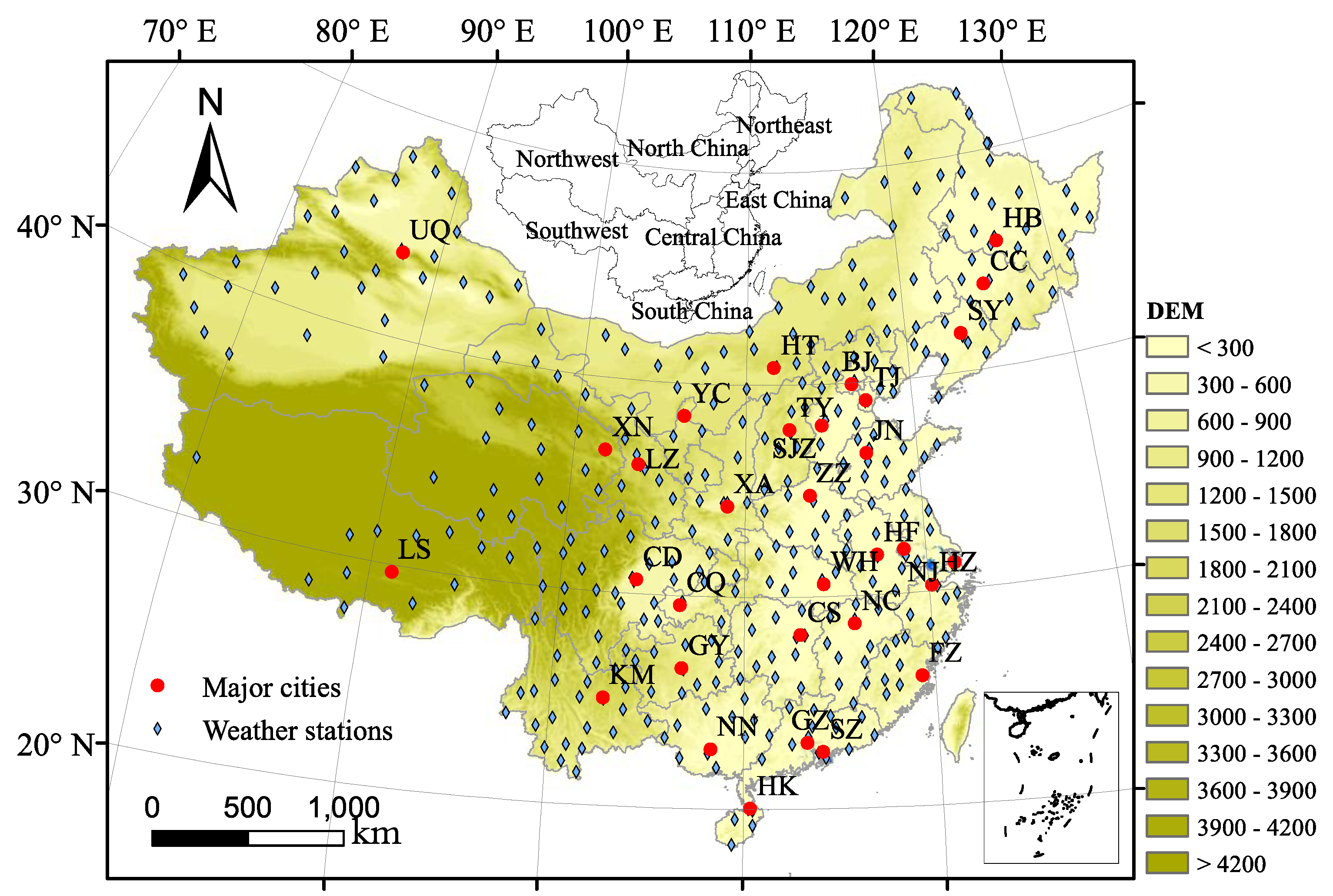
This article focuses on 32 major cities in China, including 31 municipalities or provincial capitals and one special economic zone (Figure 1). MODIS collection-5 products of LST (703 images), enhanced vegetation index (EVI, 228 images), land-use land-cover (LULC, 19 images), and surface shortwave albedo (456 images) were collected in 2009. These satellite data are of high quality and are widely used [17,27,28]. The MODIS instruments on board both the Aqua and Terra Spacecraft platforms can obtain the image of the entire Earth surface with a revisit period of 1 to 2 d. The 8-d mean LST products (MYD11A2) including daytime (~13:30) and nighttime (~01:30) temperature were used. The LST data generally had an absolute bias of less than 1 K [27]. The MODIS monthly EVI products (MOD13A3) were used to reflect vegetation activity. The MODIS yearly LULC data (MCD12Q1) were used to distinguish urban pixels. The MODIS albedo products (MCD43B3) including black sky albedo (BSA) and white sky albedo (WSA) over shortwave broadband (0.3–3.0 μm) were collected. Because the BSA is linearly correlated with WSA [4], only WSA was applied in this study. The MODIS LST, EVI, and albedo cover China with a spatial resolution of 1 km. The MODIS surface reflectance and LULC products (MOD09A1) cover China with a spatial resolution of 500 m. A digital elevation model (DEM, 62 images) was obtained from the Consultative Group on International Agricultural Research (CGIAR) consortium for spatial information with a spatial resolution of approximately 90 m. The Defense Meteorological Satellite Program (DMSP) Operational Linescan System (OLS) nighttime lights (1 image) were available from the US National Oceanic and Atmospheric Administration (NOAA). All data were resampled to 1 km spatial resolution using bilinear interpolation, and were merged into monthly composites. The NOAA’s National Centers for Environmental Information (NCEI, https://gis.ncdc.noaa.gov/) provides access to global weather data. A total of 370 weather station data sets were collected (Figure 1). The weather data records the hourly/sub-hourly SAT. We used SAT observed at 02:00 and 14:00 to match the observation times of LST data.
2.2. Methods
2.2.1. Near-Surface Air Temperature Estimation and Evaluation
The underlying relationships among SAT, LST, and auxiliary data have been widely investigated for estimating SAT distributions [29,30]. The LST, a surface parameter significantly affected by the land cover, plays the most important role in the estimation of SAT [31,32,33]. In addition, a large amount of auxiliary data was used to improve the model performance, e.g., DEM [30,31], normalized difference vegetation index (NDVI) [32], nighttime lights [34]. These data have been used well to characterize the spatial pattern of SAT and also the change on time [33]. Random forest, an algorithm establishing multiple decision trees and merges them together for more accurate and stable predictions, was found to produce more accurate SAT distributions compared with ordinary least squares regression and support vector machine methods [31]. The algorithm can avoid the problem of multicollinearity faced by general regression analysis, with the ability to reach rapid convergence and confer strong generalization [35]. It has been applied to good effect in both large-scale and fine-scale SAT mapping [12,34]. Here, we used random forest regression models implemented in R language of version 3.4.3 (https://www.r-project.org/) to map monthly mean daytime (14:00) and nighttime (02:00) SAT based on EVI, nighttime lights, LULC, DEM, and daytime and nighttime LST data [34]. Quality reports from these products indicated that cloud-contaminated pixels had been removed. Therefore, monthly SAT at pixel level was only obtained in areas with clear sky days. First, we integrated daily hourly SAT (i.e., daytime: 14:00 and nighttime: 02:00) into monthly mean hourly SAT to maintain consistency with satellite data. Next, SAT observations as response variable, and EVI, nighttime lights, LULC, DEM, and daytime and nighttime LST as regression variables, were applied to random forest regression models to predict daytime and nighttime SAT over the entire study area. The sample was divided into 90% training sets and 10% validation sets. Training sets were used to establish the relationships between variables. Validation sets were used to evaluate model accuracy. A 10-fold cross-validation was conducted to obtain stable models. The standard deviation, mean absolute error (MAE) and root mean square error (RMSE) were used to evaluate model performance.
2.2.2. Quantifying CLHII along Urban-Rural Gradients
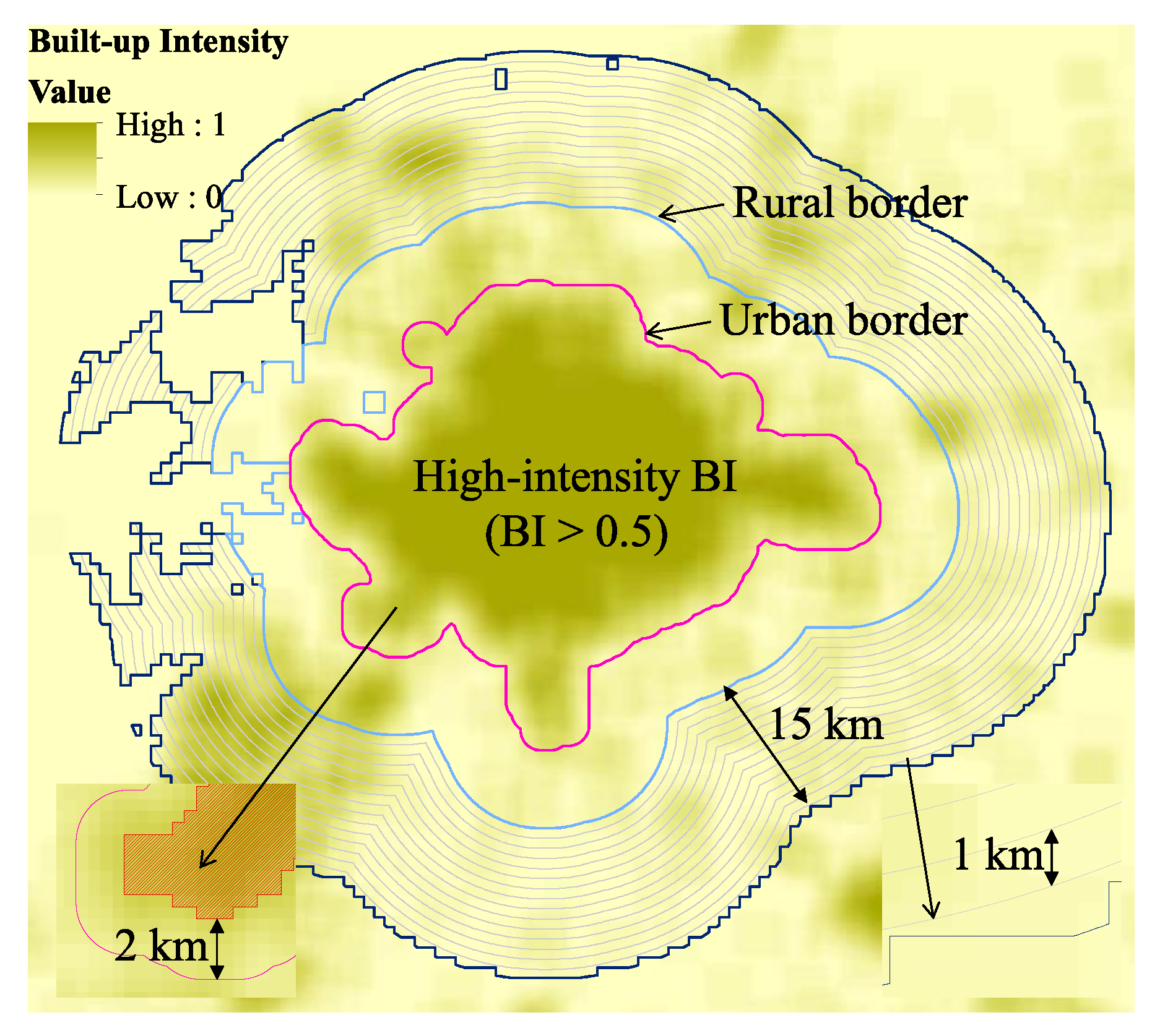
Yearly MODIS LULC map regions were grouped into seven types (i.e., forest, grassland, cropland, water, urban, bare ground, and snow) that used to distinguish urban coverage. We followed the steps below to define urban and surrounding rural areas [17]. First, we generated a BI map from impervious surface (i.e., the surface mainly covered by impenetrable materials such as asphalt, concrete, brick, stone) extracted from MODIS land cover map based on a 1 km × 1 km moving window method. Next, we selected a 50% BI threshold to divide the BI maps into high-intensity and low-intensity BI polygons [15]. Then, we aggregated the high-intensity BI polygons and then created a buffer distance of 2 km to delineate the urban border. We defined a rural area as a buffer area around an urban area, with the same size as the urban area [17]. In particular, we excluded water pixels and those pixels with altitudes exceeding 50 m above the highest point in the urban areas, since it may overshadow the effects of urbanization on local temperature [15,36]. For each city, 15 km buffers, in 1 km intervals, emanating outwards from the surrounding suburban areas to the outer suburbs were created to calculate UHI intensity along urban-rural gradients. The way of regional division is shown in Figure 2.
Previous studies have used LST differences between urban and rural areas to calculate the SUHII [4]. Generally, this method is more objective in comparison with previous analyses using a point a certain distance away from the urban area as its reference location [15,16], yet it fails to calculate the CLHII due to an obvious CLHI footprint along urban–rural gradients [12]. On this basis, we defined the CLHII and SUHII as the difference between urban temperature (the average temperature over an urban area as a bulk, without considering internal variations in a city) and the median of temperature in the outermost buffer zones (i.e., the background temperature), because it can reduce the possible bias caused by the outliers among the three outermost buffer zones [36]. We calculated the temperature difference (∆Tn) in each buffer area and the surrounding rural temperature as follows:
where ∆Tn is the temperature difference between the buffern and the background area; Tn is the temperature in buffern; Trural is the rural temperature around the urban area (i.e., background temperature). Among them, ∆T0 represents CLHII or SUHII in the urban area.
ΔTn = Tn − Trural,
2.2.3. Quantifying the Potential Drivers of CLHI
Vegetation parameter, surface physical parameters, and two density parameters were defined to explain the CLHII’s spatial variations. The vegetation parameter is calculated as the difference in EVI (δEVI) between urban and rural areas. Surface physical parameters were calculated by the difference in surface albedo (δAlbedo) between urban and rural areas. Density parameters include nighttime lights and BI. In addition, we linked SUHI to CLHI effects across China’s 32 major cities. Each of the buffers was a unit of statistical data and was used for correlation analysis. We calculated annual and seasonal CLHII during 2009 for each city. Seasonal changes were tested in spring (March–May), summer (June–August), autumn (September–November), and winter (December–February). Linear regression was used to analyze the relationships between CLHII and the variables used in this study across multiple cities.
3. Results
3.1. Spatial Pattern of CLHII and SUHII
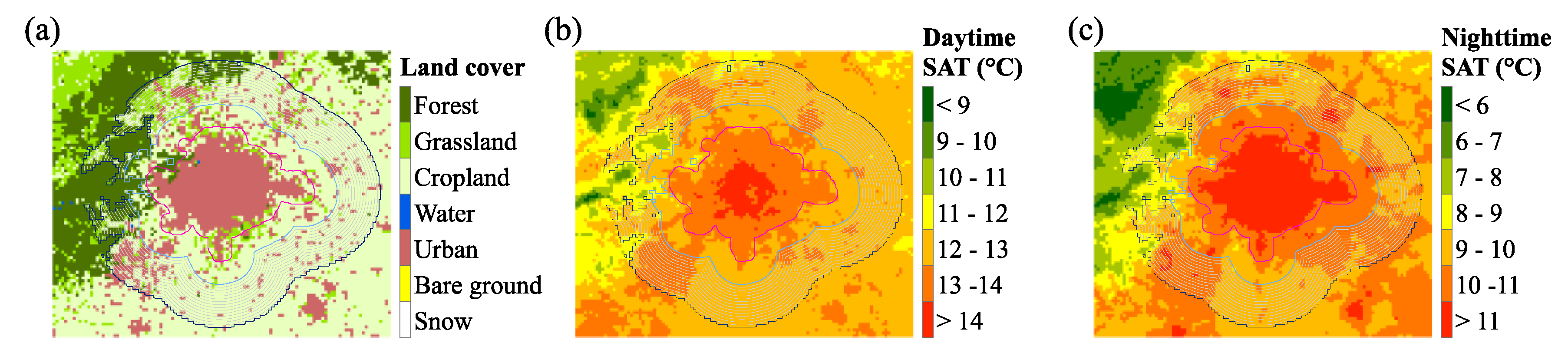
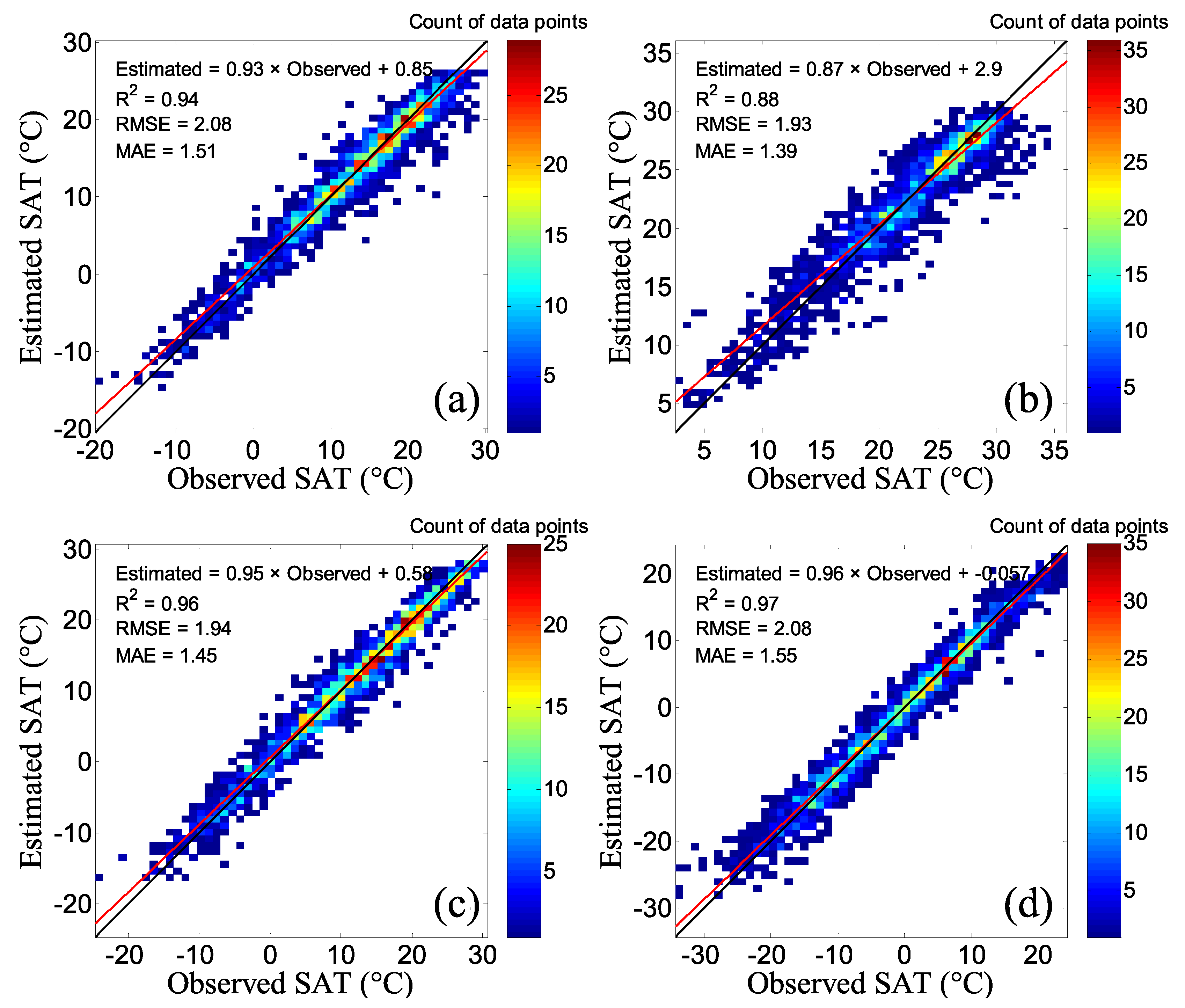
Figure 3a shows the land cover and Figure 3b,c shows sthe spatial distribution of SAT during the day and night in the Beijing metropolitan area. Apparently, the SAT in urban pixels was higher than in other areas during both day and night in Beijing, presenting a clear CLHI effect. Figure 4 shows the prediction errors of the regression model used to map SAT. The standard deviations of the observed SAT were 8.6 °C, 5.6 °C, 10.2 °C, and 11.1 °C in spring, summer, autumn, and winter, respectively. These standard deviations were significantly larger than the corresponding RMSE (Figure 4). Also, the cross-validation R2 ranged from 0.88 in summer to 0.97 in winter. These results indicate that the retrieval algorithm of SAT was accurate. The method presented in this article significantly improves the spatial scale and accuracy of CLHI monitoring, compared to the case study (R2 = 0.53) in Wuhan city, China [12].
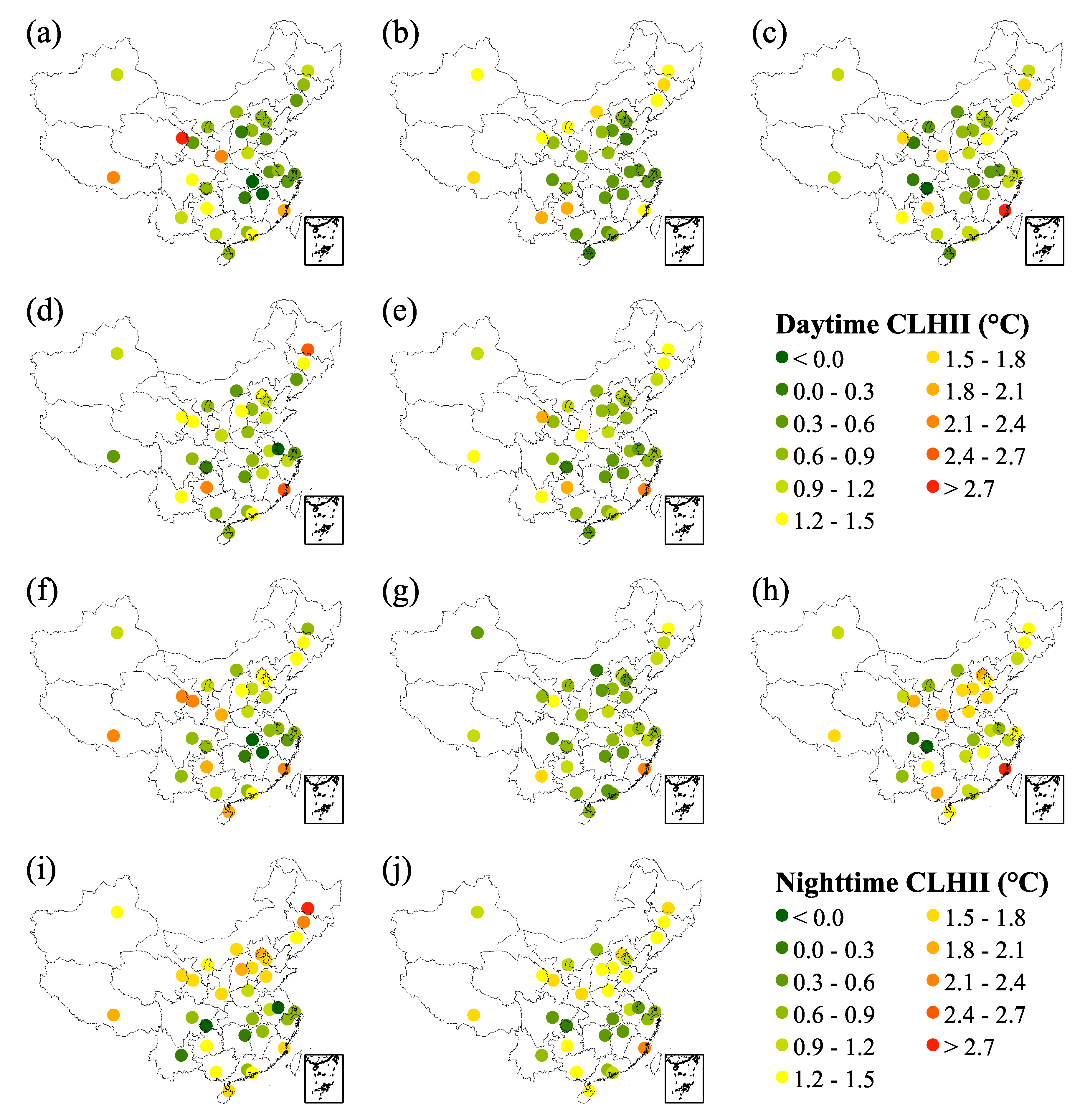
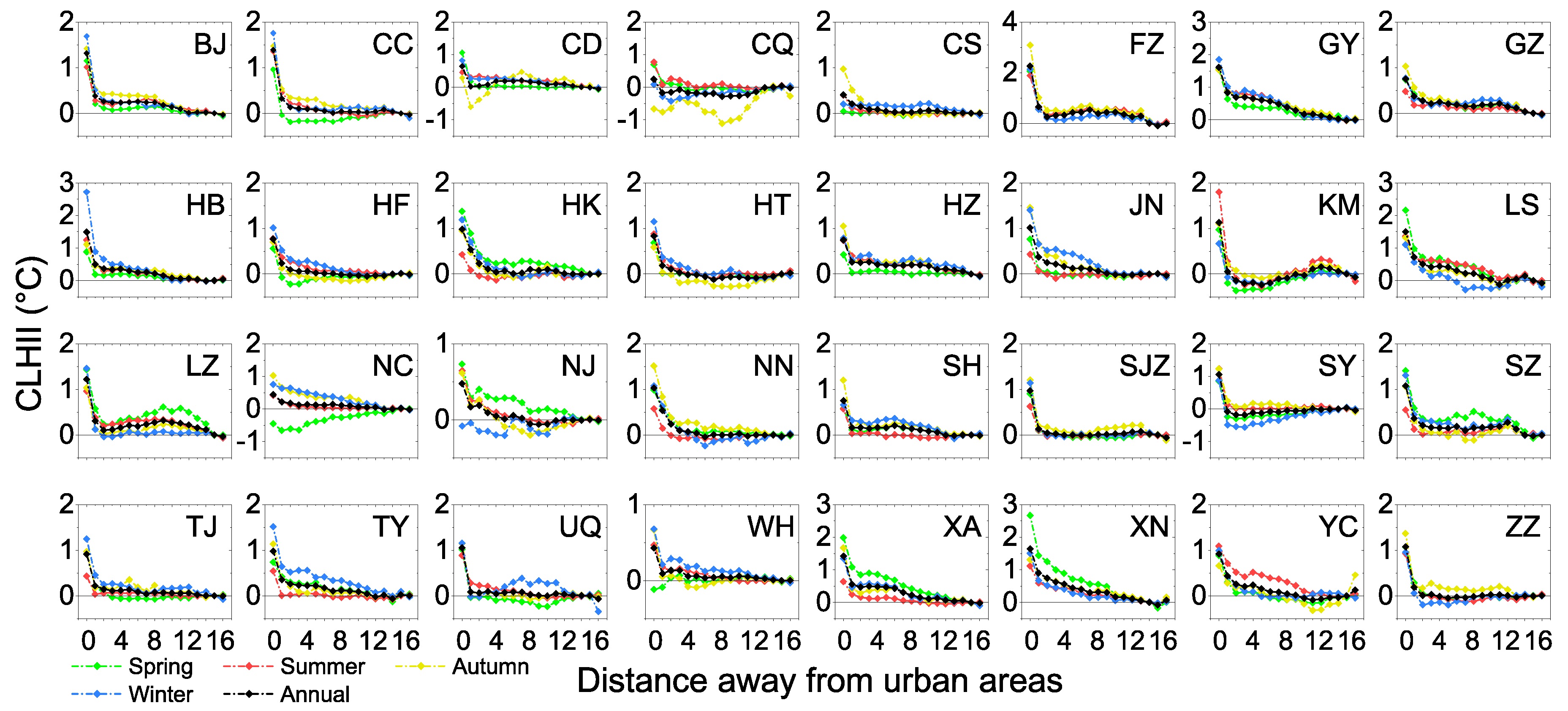
Both the annual daytime and nighttime CLHIIs were positive for these 32 major cities, which ranged from 0.2 °C to 2.2 °C in the day and from 0.3 °C to 2.4 °C in the night, respectively (the weakest CLHI in Chongqing and the strongest CLHI in Fuzhou in both day and night). The CLHII during the day varied irregularly in space, presenting a higher annual CLHII in the northeast, northwest, and southwest. During the night, the major cities located in the north of China (Northeast, Northwest, and North China) experienced more intense annual CLHII (Table 1). Diurnal variation shows that the CLHII is generally higher in the night, especially for northern parts of China (Figure 5). This asymmetrical diurnal variation had a consistent trend with SUHII in that nighttime SUHII in the northern parts of China tends to be higher [17]. Seasonal variation shows that the Southwest tends to present a higher CLHII in summer during both day and night (Table 1, Figure 5). Coastal cities showed a weaker CLHI effect compared to that above inland cities possibly due to the influence of atmosphere circulation. Figure 6 shows the SAT difference between urban buffers and background areas. It is found that urban and surrounding areas had higher SAT than rural areas, and the CLHI effect had an exponential decay shape along urban–rural gradients, which is the same as the trends seen along urban-rural gradients in SUHII observed in previous studies [36]. In addition, the difference in CLHII was apparent among both cities and seasons (Figure 6). For instance, Chongqing experienced a canopy layer cool island effect in autumn. This cool island effect was also observed in Nanchang and Wuhan in spring and Nanjing in winter (Figure 6).
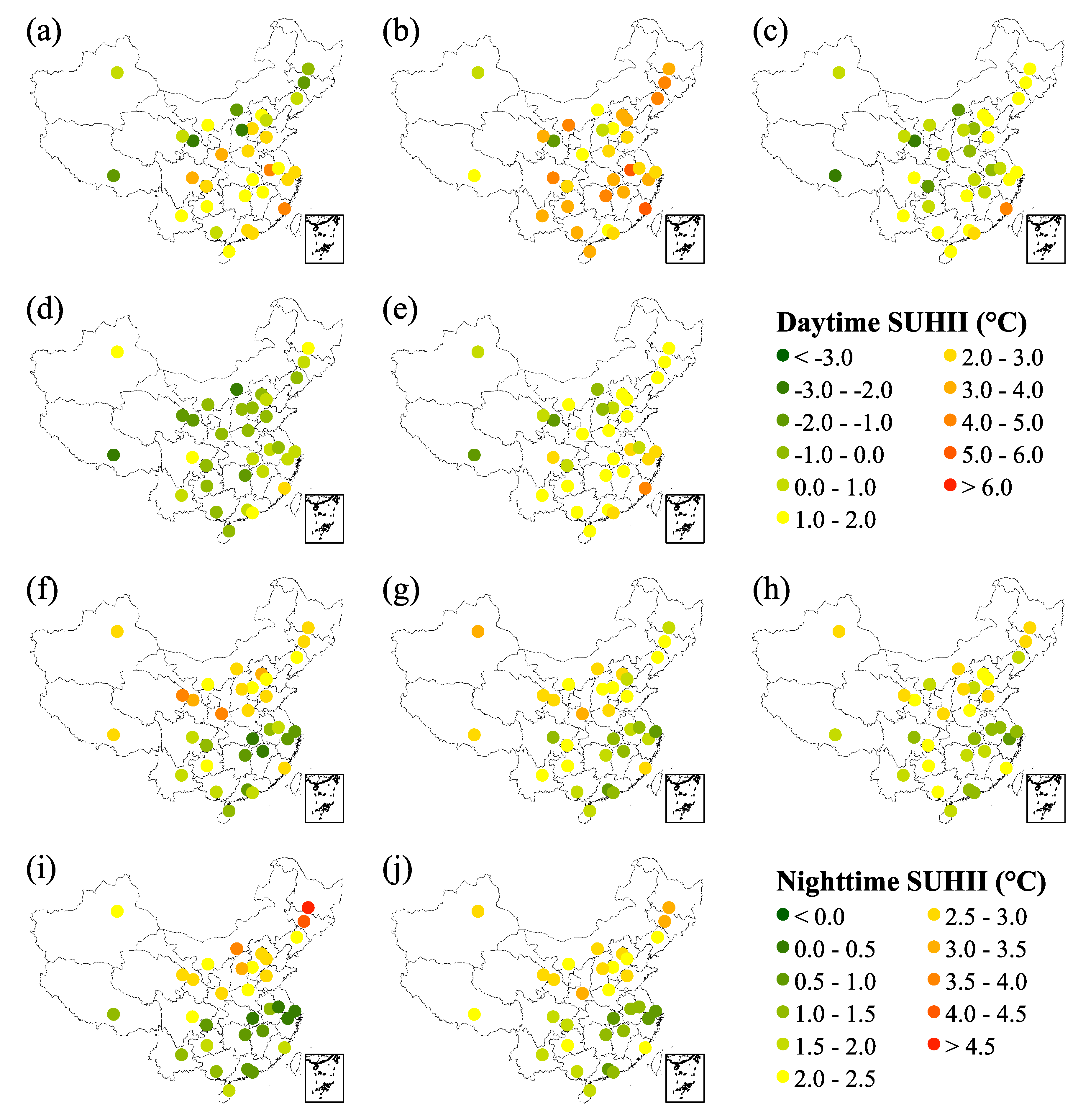
Figure 7 shows the spatial pattern of SUHII for 32 major cities. The annual mean daytime and nighttime SUHII had regional differences, which ranged from −2.0 (Lanzhou) to 4.3 (Fuzhou), and 0.7 (Wuhan) to 3.2 (Harbin), respectively. The negative (Lanzhou) and low (Wuhan) values may be due to the influence of water environment, as the Lanzhou is the only provincial capital to cross the Yellow River, and the water area in Wuhan accounts for nearly 1/4 of the total area of city. On the whole, more intense daytime SUHII was observed in cities located in the northeast, east, and southern regions of China, compared with those in the northwest and southwest. In contrast, a higher nighttime SUHII was observed in the cities located in the northern and southwest parts of China, compared to those in the southern and eastern regions. There were obvious seasonal variations in the spatial patterns of SUHII, especially for the daytime SUHII. Most of the cities experienced more intense daytime SUHII in summer compared to those in winter. At all seasons, most of the cities had more intense nighttime SUHII in northern China. This spatial pattern of SUHII in both day and night is consistent with the result of previous studies [17].
3.2. Drivers of Spatial Variation in CLHI
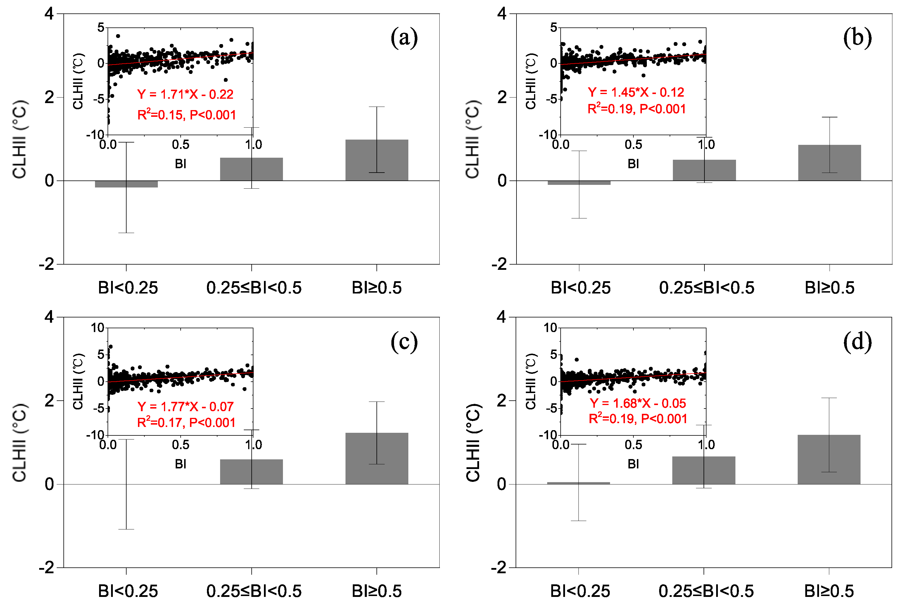
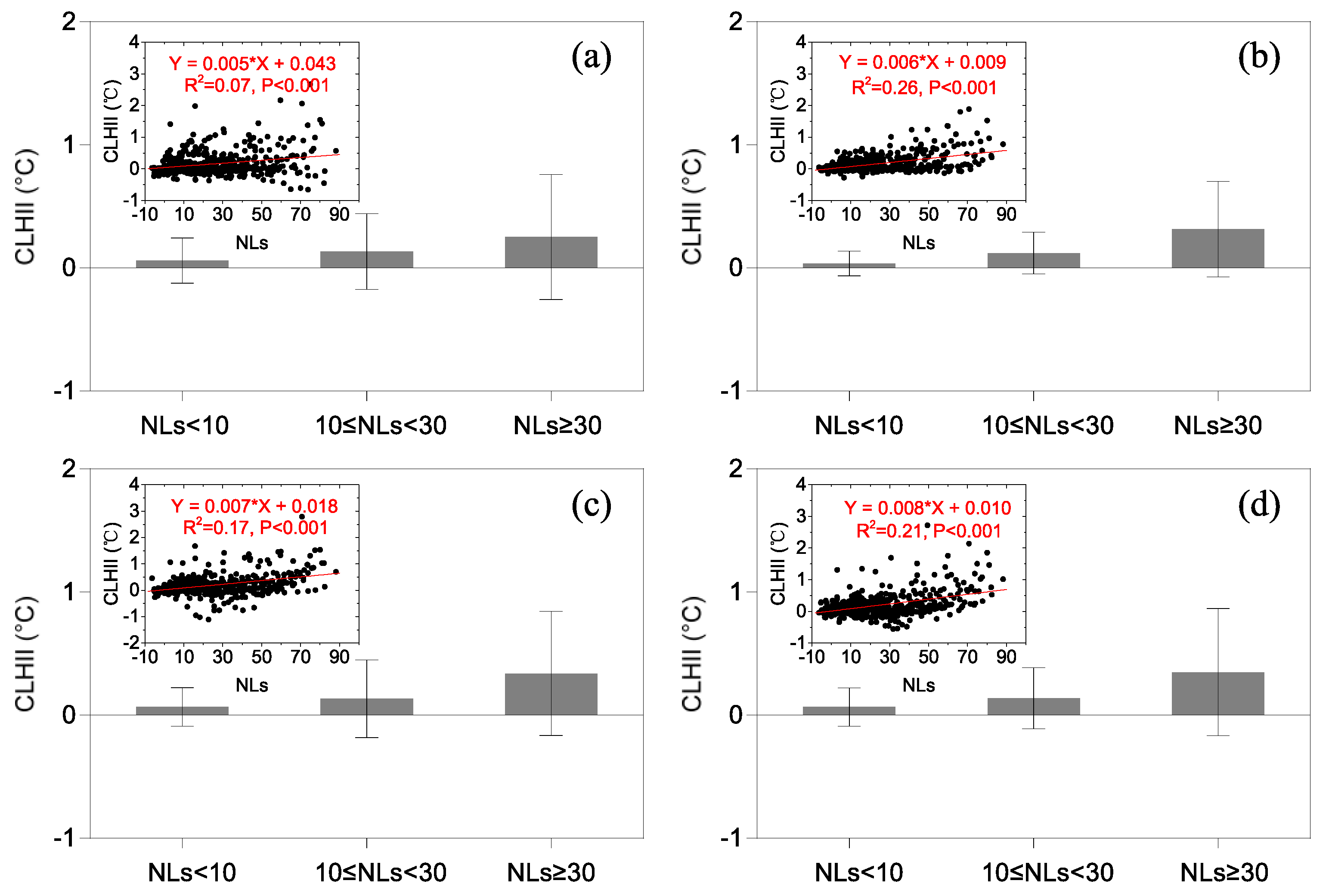
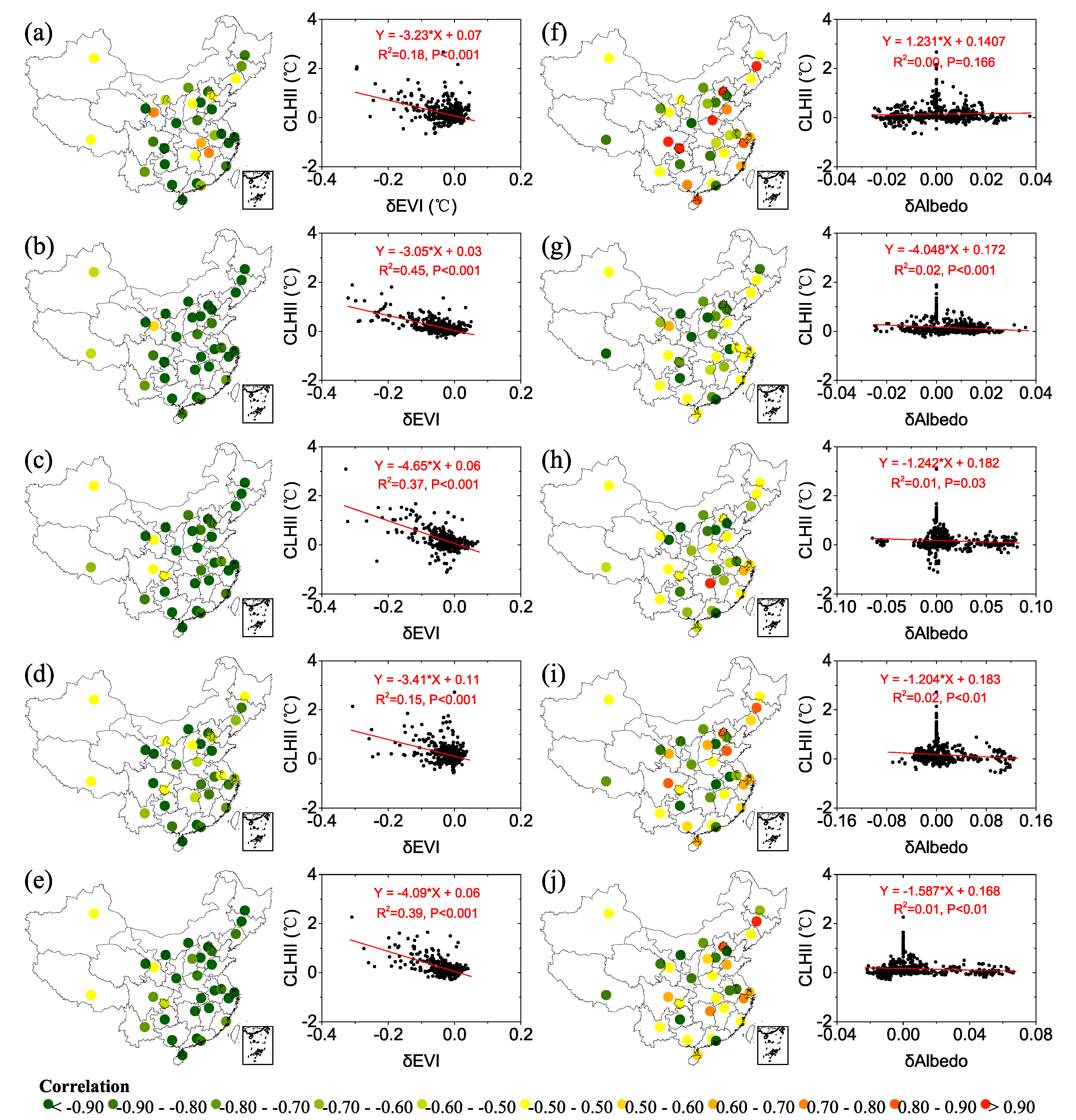
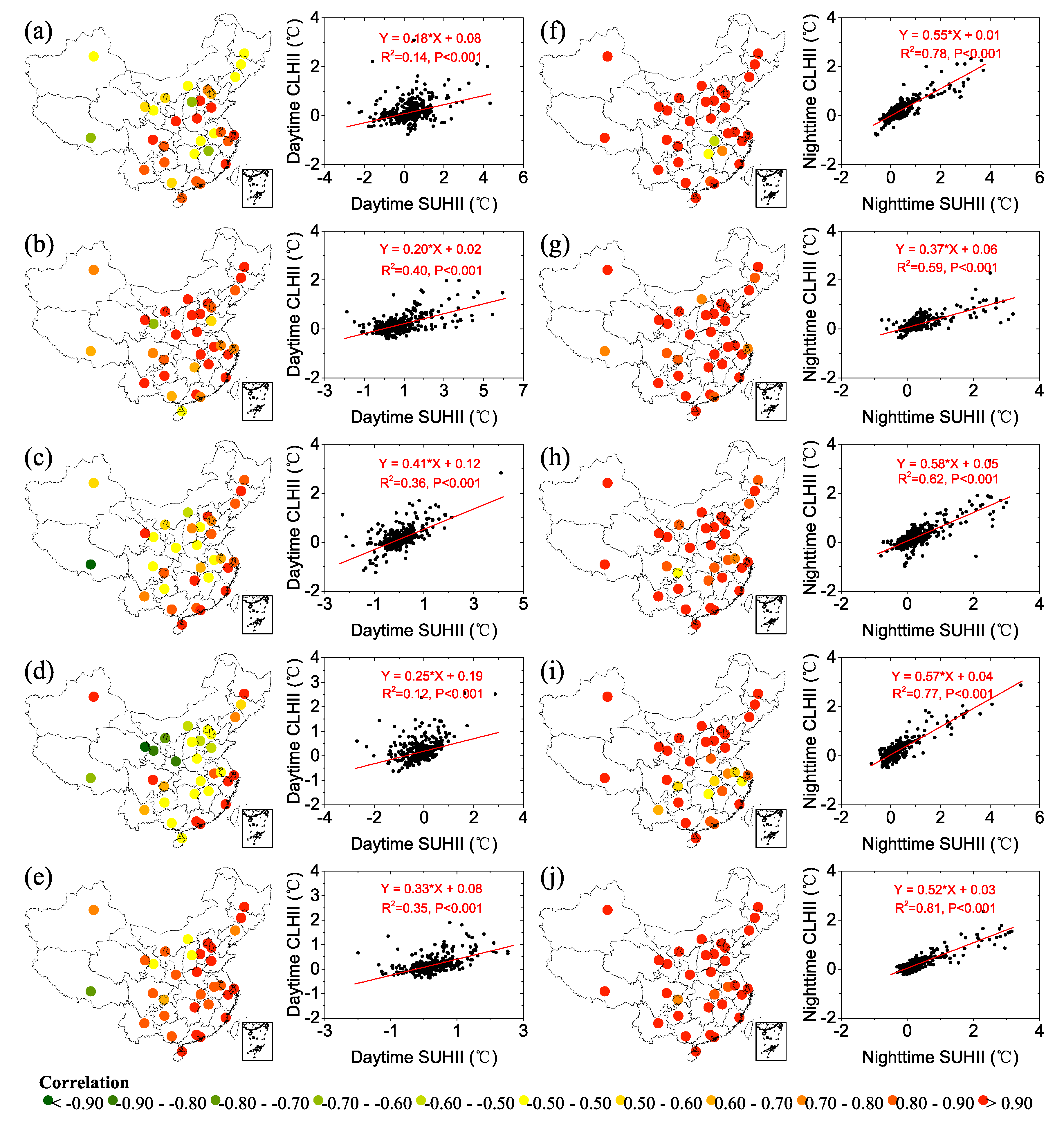
Figure 8 shows that BI had significant and positive effects on CLHII, with a small seasonal variation (significance level p < 0.001), indicating that the urban areas having high BI tend to have more intense CLHII. The nighttime lights correlated significantly and positively to the CLHII, which suggests that higher anthropogenic emissions exacerbate the CLHI effect, especially in summer and winter (Figure 9). Additionally, the relationship of CLHII with vegetation and surface albedo are shown in Figure 10; compared with winter (R2 = 0.15, p < 0.001), vegetation activity was correlated more strongly and negatively to the CLHII in summer (R2 = 0.45, p < 0.001). Compared with other seasons, surface albedo was correlated more strongly and negatively to the CLHII in summer and winter, but presents very low correlations. (R2 = 0.02, p < 0.01). Most of the cities showed significant and positive correlation with daytime and nighttime SUHII (Figure 11). In particular, most cities had a stronger correlation between CLHII and SUHII during the day in summer (Figure 11a–d), and during nighttime in other seasons (Figure 11f–i).
4. Discussion
4.1. Possible Drivers Controlling CLHII Spatial Patterns
The SUHII was driven by different variables, such as vegetation activity, surface albedo, anthropogenic heat emissions, and BI [17]. These variables control the surface energy balance by changing the heat fluxes [37]. Our results indicated that CLHII has strong correlations with SUHII, particularly during the night. The possible mechanisms controlling CLHII are discussed below.
4.1.1. Built-Up Intensity
There were significant and positive correlations between CLHII and BI, and the relationships had small seasonal variations (Figure 8). We conclude that BI aggravates the CLHII by significantly increasing the burden on surface, resulting in more heat storage at the surface and more heat release in the form of sensible heat flux to atmosphere. A possible reason for this could be higher BI is expected to help maintain warmer temperatures than those in areas with lower BI, because this heat can be emitted by human activities and is stored by buildings and roads in urban areas [17,38,39] thus increasing the burden on the CLHI effect.
4.1.2. Nighttime Lights
Nighttime lights are used as a proxy for socio-economic activities [40,41], and are also considered as a proxy for anthropogenic heat emissions [17,42]. The anthropogenic heat flux released into the atmosphere directly affects the local temperature. This part of the heat also can be converted into sensible heat flux [43], and contribute to maintaining the SUHII, particularly during the night [4]. We find significant and positive correlation between CLHII and nighttime lights (Figure 9), especially in summer and winter. This positive correlation between CLHII and nighttime lights is analogous to the studies of SUHII [4,17,39]. Therefore, we suggest the important role of anthropogenic heat emissions on the CLHI effect. This correlation between CLHII and nighttime lights is better than that with SUHII, implying the more direct influence of anthropogenic emissions on the CLHI effect compared to SUHI effect.
4.1.3. Vegetation Activity
Vegetation increasing the latent heat flux via evaporation is expected to have a cooling effect compared with impervious surfaces, and hence offers potential for mitigation of SUHI effects [4,16,23]. In addition, vegetation correlated significantly and negatively to the CLHII in both summer and winter [12]. Our results show obvious spatial and seasonal variations in the relationships between CLHII and δEVI (Figure 10). Furthermore, our results support the mechanism by which vegetation mitigates the CLHI effect, through transpiration releasing water vapor, thus increasing the latent heat flux. The vegetation feedback is more significant in summer and weakly in winter, which is attributed to the phenology that vegetation undergoes more evaporation during the mature period compared to that in periods of plant growth and senescence.
4.1.4. Surface Albedo
The proportion of impervious surfaces continues to increase as a result of rapid urbanization, resulting in lower emissivity and surface albedo in urban areas. Together, the new materials used in urban areas reduce heat loss because they can absorb more all-wavelength radiation and have a higher heat-storage capacity [37,38]. The nighttime SUHII is generally driven by the surface heat fluxes absorbed in the daytime [37], and hence those cities with larger and negative surface albedo difference between urban and background areas (i.e., a larger and negative δAlbedo) are expected to experience more intense SUHII at night. The surface albedo has a more significant effect in winter compared to summer owing to defoliation and snow-cover [17]. In contrast, to confirm the difficult to interpret the δAlbedo in a heterogeneous and variable scenario (urban and rural), research found that the δAlbedo contributed little to the SUHI in Chinese cities both in spatial patterns and seasonal trends [44]. Similar to the results from Zhou et al. [44], our results show that the impacts of surface albedo to CLHII disappeared (Figure 10), given that this correlation is very low. In other words, our result shows a loss of correlation with SAT, which is consistent with the results as reported in Baldinelli et al. [45]. In fact, the relationship between surface albedo and SAT is not simple, due to the impact of the vegetation (low albedo), present both in the urban and rural areas, as well as the seasonal variation. Also, when the micro-scale heat transfer effect is high, their correlation disappears [45].
4.2. Spatial Distribution of CLHII and Their Potential Drivers
The spatial distribution of CLHII was affected by physical mechanism, presenting diurnal and seasonal variations (Figure 5). The annual daytime CLHII was explained by greater vegetation cover in the southwest [17], and also in the northeast, and northwest (Figure 10, Table 1). During the night, more intense annual CLHII in the northern parts of China, could be explained by low soil moisture and strong positive feedback arising from the LST (Figure 7 and Figure 11). A higher CLHII was observed in the southwest in summer, which was mainly explained by the strong vegetation feedback (Figure 10). Both nighttime lights and BI aggravated CLHII (Figure 8 and Figure 9). A few cities experienced a canopy layer cool island effect (Figure 6). For instance, there is a canopy layer cool island effect observed in Chongqing in the autumn (Figure 6), which could be explained by the weak vegetation feedback (Figure 10c).
4.3. Relationship between CLHI and SUHI Effects
The SUHII is generally thought to be biophysical in nature, arising from the difference of surface properties between urban and rural land, including sensible heat convection efficiency, evaporative cooling, sunlight reflection, and anthropogenic heat emissions [46,47]. We find that most of the cities presented strong correlations between CLHII and SUHII, particularly at night (Figure 11). The annual daytime SUHII (~13:30) explained 35% of the variation in annual daytime (14:00) CLHII. The annual nighttime SUHII (~01:30) explained 81% of the variation in annual nighttime (02:00) CLHII (Figure 11). These results indicated that the SUHI effect correlated significantly to the CLHI effect, which is consistent with a case study in Milan, in which SAT and LST show a correlation coefficient greater than 0.95 at night and a correlation coefficient of less than 0.6 during the day [48]. Furthermore, the annual daytime SUHII was 1.2 ± 1.1 °C with 0.40 °C (Figure 11, 95% confidence interval 0.36 to 0.44 °C) of annual daytime CLHII observed in urban areas. The annual nighttime SUHII was 2.0 ± 0.8 °C, accompanied by 1.04 °C (Figure 11, 0.99–1.09 °C) of annual nighttime CLHII. In addition, the daytime and nighttime SUHII explained 40% and 59% of the variation in CLHII during summer, respectively. In contrast, the daytime and nighttime SUHII explained 12% and 77% of the variation in CLHII in winter. The difference in correlation resulting from diurnal and seasonal variations can be interpreted as arising from heat storage in daytime and heat release at night, and more heat being absorbed in summer compared to winter.
5. Conclusions
This study quantified the spatial pattern, diurnal and seasonal variations in CLHI effect and its drivers in China’s 32 major cities. Both the annual daytime and nighttime CLHII were positive ranging from 0.2 °C to 2.2 °C and from 0.3 °C to 2.4 °C in China’s 32 major cities, respectively. The cities located in Northern China experienced more intense CLHII, particularly at night. In addition, the CLHI effect had an exponential decay shape along urban–rural gradients. Nighttime lights and BI had positive effects on the CLHII. Vegetation correlated negatively, and more strongly, to the CLHII in summer. Surface albedo showed an extremely weak correlation with the CLHII. In particular, we provided a method to link CLHI to SUHI effects across China’s 32 major cities, and indicated that CLHII had strong correlations with SUHII, implying the mitigation of SUHI effect provides a co-benefit in mitigating CLHI effect. In summary, this research provides a new CLHI monitoring process and can be used to guide further studies across other cities. However, in reality, the air temperature can be influenced by advection, so that CLHII can depend on the wind and atmospheric stability. Some studies have shown that wind speed affects surface–atmospheric interactions, causing attenuation of UHI effect [49,50]. Therefore, it is necessary to consider more meteorological parameters to better understand the spatiotemporal variation of CLHI effect in future studies.
Author Contributions
Conceptualization, L.L.; Data curation, L.L.; Formal analysis, L.L.; Funding acquisition, L.L. and Y.Z.; Methodology, L.L.; Writing – original draft, L.L.; Writing – review & editing, L.L. and Y.Z.
Funding
This research was funded by the Postgraduate Research & Practice Innovation Program of Jiangsu Province (Grant #: KYCX18_1203), and the National Natural Science Foundation of China (Grant #: 41671428).
Acknowledgments
We thank all reviewers for their comments towards improving the technical quality of the manuscript.
Conflicts of Interest
The authors declare no conflict of interest.
References
- Grimm, N.B.; Faeth, S.H.; Golubiewski, N.E.; Redman, C.L.; Wu, J.; Bai, X.; Briggs, J.M. Global change and the ecology of cities. Science 2008, 319, 756–760. [Google Scholar] [CrossRef] [PubMed]
- United, N. World Urbanization Prospects: The 2009 Revision; Department of Economic and Social Affairs, Population Division: New York, NY, USA, 2009. [Google Scholar]
- Zhou, L.M.; Dickinson, R.E.; Tian, Y.H.; Fang, J.Y.; Li, Q.X.; Kaufmann, R.K.; Tucker, C.J.; Myneni, R.B. Evidence for a significant urbanization effect on climate in China. Proc. Natl. Acad. Sci. USA 2004, 101, 9540–9544. [Google Scholar] [CrossRef] [PubMed] [Green Version]
- Peng, S.; Piao, S.; Ciais, P.; Friedlingstein, P.; Ottle, C.; Bréon, F.M.; Nan, H.; Zhou, L.; Myneni, R.B. Surface urban heat island across 419 global big cities. Environ. Sci. Technol. 2012, 46, 696. [Google Scholar] [CrossRef] [PubMed]
- Kalnay, E.; Cai, M. Impact of urbanization and land-use change on climate. Nature 2003, 42, 528–531. [Google Scholar] [CrossRef] [PubMed]
- Georgescu, M.; Morefield, P.E.; Bierwagen, B.G.; Weaver, C.P. Urban adaptation can roll back warming of emerging megapolitan regions. Proc. Natl. Acad. Sci. USA 2014, 111, 2909–2914. [Google Scholar] [CrossRef] [PubMed] [Green Version]
- Santamouris, M. Heat Island Research in Europe: The State of the Art. Adv. Build. Energy Res. 2007, 1, 123–150. [Google Scholar] [CrossRef]
- Zhao, L.; Lee, X.; Smith, R.B.; Oleson, K. Strong contributions of local background climate to urban heat islands. Nature 2014, 511, 216–219. [Google Scholar] [CrossRef]
- Giannaros, C.; Nenes, A.; Giannaros, T.M.; Kourtidis, K.; Melas, D. A comprehensive approach for the simulation of the Urban Heat Island effect with the WRF/SLUCM modeling system: The case of Athens (Greece). Atmos. Res. 2018, 201, 86–101. [Google Scholar] [CrossRef]
- Zhang, X.; Friedl, M.A.; Schaaf, C.B.; Strahler, A.H.; Schneider, A. The footprint of urban climates on vegetation phenology. Geophys. Res. Lett. 2004, 31, 179–206. [Google Scholar] [CrossRef]
- Tan, J.; Zheng, Y.; Tang, X.; Guo, C.; Li, L.; Song, G.; Zhen, X.; Yuan, D.; Kalkstein, A.J.; Li, F.; et al. The urban heat island and its impact on heat waves and human health in Shanghai. Int. J. Biometeorol. 2010, 54, 75–84. [Google Scholar] [CrossRef]
- Li, L.; Huang, X.; Li, J.; Wen, D. Quantifying the spatiotemporal trends of Canopy Layer Heat Island (CLHI) and its driving factors over Wuhan, China with satellite remote sensing. Remote Sens. 2017, 9, 536. [Google Scholar] [CrossRef]
- Pichierri, M.; Bonafoni, S.; Biondi, R. Satellite air temperature estimation for monitoring the canopy layer heat island of Milan. Remote Sens. Environ. 2012, 127, 130–138. [Google Scholar] [CrossRef]
- Gaur, A.; Eichenbaum, M.K.; Simonovic, S.P. Analysis and modelling of surface urban heat island in 20 Canadian cities under climate and land-cover change. J. Environ. Manag. 2017, 206, 145–157. [Google Scholar] [CrossRef] [PubMed]
- Imhoff, M.L.; Zhang, P.; Wolfe, R.E.; Bounoua, L. Remote sensing of the urban heat island effect across biomes in the continental USA. Remote Sens. Environ. 2010, 114, 504–513. [Google Scholar] [CrossRef] [Green Version]
- Tran, H.D.; Uchihama, S.O.; Yasuoka, Y. Assessment with satellite data of the urban heat island effects in Asian mega cities. Int. J. Appl. Earth Obs. 2006, 8, 34–48. [Google Scholar] [CrossRef]
- Zhou, D.; Zhao, S.; Liu, S.; Zhang, L.; Chao, Z. Surface urban heat island in China’s 32 major cities: Spatial patterns and drivers. Remote Sens. Environ. 2014, 152, 51–61. [Google Scholar] [CrossRef]
- Koken, P.J.M.; Piver, W.T.; Ye, F.; Elixhauser, A.; Olsen, L.M.; Portier, A.C.J. Temperature, air pollution, and hospitalization for cardiovascular diseases among elderly people in denver. Environ. Health Perspect. 2003, 111, 1312. [Google Scholar] [CrossRef] [PubMed]
- Vandentorren, S.; Bretin, P.; Zeghnoun, A.; Mandereau-Bruno, L.; Croisier, A.; Cochet, C.; Riberon, J.; Siberan, I.; Declercq, B.; Ledrans, M. August 2003 heat wave in France: Risk factors for death of elderly people living at home. Eur. J. Public Health 2006, 16, 583–591. [Google Scholar] [CrossRef]
- Goggins, W.B.; Chan, E.Y.Y.; Ng, E.; Ren, C.; Chen, L. Effect modification of the association between short-term meteorological factors and mortality by urban heat islands in Hong Kong. PLoS ONE 2012, 7, 9–14. [Google Scholar] [CrossRef]
- Smargiassi, A.; Goldberg, M.S.; Plante, C.; Fournier, M.; Baudouin, Y.; Kosatsky, T. Variation of daily warm season mortality as a function of micro-urban heat islands. J. Epidemiol. Community Heal. 2009, 63, 659–664. [Google Scholar] [CrossRef] [Green Version]
- Tomlinson, C.J.; Chapman, L.; Thornes, J.E.; Backer, C.J. Derivation of Birmingham’s summer surface urban heat island from MODIS satellite images. Int. J. Climatol. 2012, 32, 214–224. [Google Scholar] [CrossRef]
- Yuan, F.; Bauer, M.E. Comparison of impervious surface area and normalized difference vegetation index as indicators of surface urban heat island effects in Landsat imagery. Remote Sens. Environ. 2007, 106, 375–386. [Google Scholar] [CrossRef]
- Huang, W.; Li, J.; Guo, Q.; Mansaray, L.R.; Li, X.; Huang, J. A satellite-derived climatological analysis of urban heat island over Shanghai during 2000–2013. Remote Sens. 2017, 9, 641. [Google Scholar] [CrossRef]
- Fabrizi, R.; Bonafoni, S.; Biondi, R. Satellite and ground-based sensors for the urban heat island analysis in the city of Rome. Remote Sens. 2010, 2, 1400–1415. [Google Scholar] [CrossRef]
- Sun, H.; Chen, Y.; Zhan, W. Comparing surface- and canopy-layer urban heat islands over Beijing using MODIS data. Int. J. Remote Sens. 2015, 36, 5448–5465. [Google Scholar] [CrossRef]
- Wan, Z. New refinements and validation of the MODIS Land-Surface Temperature/Emissivity products. Remote Sens. Environ. 2008, 112, 59–74. [Google Scholar] [CrossRef]
- Schaaf, C.B.; Gao, F.; Strahler, A.H.; Lucht, W.; Li, X.; Tsang, T.; Strugnell, N.C.; Zhang, X.; Jin, Y.; Muller, J.-P.; Lewis, P.; et al. First operational BRDF, albedo nadir reflectance products from MODIS. Remote Sens. Environ. 2002, 83, 135–148. [Google Scholar] [CrossRef] [Green Version]
- Benali, A.; Carvalho, A.C.; Nunes, J.P.; Carvalhais, N.; Santos, A. Estimating air surface temperature in Portugal using MDOIS LST data. Remote Sens. Environ. 2012, 124, 108–121. [Google Scholar] [CrossRef]
- Chen, F.; Liu, Y.; Liu, Q.; Qin, F. A statistical method based on remote sensing for the estimation of air temperature in China. Int. J. Climatol. 2015, 35, 2131–2143. [Google Scholar] [CrossRef]
- Ho, H.C.; Knudby, A.; Sirovyak, P.; Xu, Y.; Hodul, M.; Henderson, S.B. Mapping maximum urban air temperature on hot summer days. Remote Sens. Environ. 2014, 154, 38–45. [Google Scholar] [CrossRef]
- Yoo, C.; Im, J.; Park, S.; Quackenbush, L.J. Estimation of daily maximum and minimum air temperatures in urban landscapes using MODIS time series satellite data. ISPRS J. Photogramm. Remote Sens. 2018, 137, 149–162. [Google Scholar] [CrossRef]
- Li, L.; Zha, Y. Satellite-based regional warming hiatus in China and its implication. Sci. Total Environ. 2019, 648, 1394–1402. [Google Scholar] [CrossRef] [PubMed]
- Li, L.; Zha, Y. Mapping relative humidity, average and extreme temperature in hot summer over China. Sci. Total Environ. 2018, 615, 875–881. [Google Scholar] [CrossRef] [PubMed]
- Breiman, L. Random forests. Mach. Learn. 2001, 45, 5–32. [Google Scholar] [CrossRef]
- Zhou, D.; Zhao, S.; Zhang, L.; Sun, G.; Liu, Y. The footprint of urban heat island effect in China. Sci. Rep. 2015, 5, 11160. [Google Scholar] [CrossRef] [Green Version]
- Arnfield, A.J. Two decades of urban climate research: A review of turbulence, exchanges of energy and water, and the urban heat island. Int. J. Climatol. 2003, 23, 1–26. [Google Scholar] [CrossRef]
- Oke, T.R. The energetic basis of the urban heat island. Q. J. R. Meteorol. Soc. 1982, 108, 1–24. [Google Scholar] [CrossRef]
- Yow, D.M. Urban heat islands: Observations, impacts, and adaptation. Geogr. Compass 2007, 1, 1227–1251. [Google Scholar] [CrossRef]
- Doll, C.H.; Muller, J.-P.; Elvidge, C.D. Night-time Imagery as a Tool for Global Mapping of Socioeconomic Parameters and Greenhouse Gas Emissions. Ambio 2000, 29, 157–162. [Google Scholar] [CrossRef]
- Elvidge, C.D.; Baugh, K.E.; Kihn, E.A.; Kroehl, H.W.; Davis, E.R.; Davis, C.W. Relation between satellite observed visible-near infrared emissions, population, economic activity and electric power consumption. Int. J. Remote Sens. 1997, 18, 1373–1379. [Google Scholar] [CrossRef]
- Sailor, D.J. A review of methods for estimating anthropogenic heat and moisture emissions in the urban environment. Int. J. Climatol. 2011, 31, 189–199. [Google Scholar] [CrossRef] [Green Version]
- Christen, A.; Vogt, R. Energy and radiation balance of a central European city. Int. J. Climatol. 2004, 24, 1395–1421. [Google Scholar] [CrossRef] [Green Version]
- Zhou, D.; Bonafoni, S.; Zhang, L.; Wang, R. Remote sensing of the urban heat island effect in a highly populated urban agglomeration area in east china. Sci. Total Environ. 2018, 628–629, 415–429. [Google Scholar] [CrossRef] [PubMed]
- Baldinelli, G.; Bonafoni, S.; Rotili, A. Albedo retrieval from multispectral landsat 8 observation in urban environment: Algorithm validation by in situ measurements. IEEE J-STARS 2017, 99, 1–8. [Google Scholar] [CrossRef]
- Oke, T.R. Boundary Layer Climates; Routledge: Abington, UK, 2002. [Google Scholar]
- Voogt, J.A.; Oke, T.R. Thermal remote sensing of urban climates. Remote Sens. Environ. 2013, 86, 370–384. [Google Scholar] [CrossRef]
- Anniballe, R.; Bonafoni, S.; Pichierri, M. Spatial and temporal trends of the surface and air heat island over Milan using MODIS data. Remote Sens. Environ. 2014, 150, 163–171. [Google Scholar] [CrossRef]
- Morris, C.J.G.; Simmonds, I.; Plummer, N. Quantification of the influences of wind and cloud on the nocturnal urban heat island of a large city. J. Appl. Meteorol. 2001, 40, 169–182. [Google Scholar] [CrossRef]
- Memon, R.A.; Leung, D.Y.C.; Liu, C.H. Effects of building aspect ratio and wind speed on air temperatures in urban-like street canyons. Build. Environ. 2010, 45, 176–188. [Google Scholar] [CrossRef]
Figure 1.
Map showing the topography of China and the location of weather stations and the 32 major cities. These cities are municipalities or provincial capitals, except a special economic zone of Shenzhen. A total of 370 weather stations from the National Weather Service (NWS) record the hourly surface air temperature (SAT). Subplot shows seven geographical divisions in China. Abbreviations: BJ, Beijing; CC, Changchun; CD, Chengdu; CQ, Chongqing; CS, Changsha; FZ, Fuzhou; GY, Guiyang; GZ, Guangzhou; HB, Harbin; HF, Hefei; HT, Hohhot; HZ, Hangzhou; JN, Jinan; KM, Kunming; LS, Lhasa; LZ, Lanzhou; NC, Nanchang; NJ, Nanjing; NN, Nanning; SH, Shanghai; SJZ, Shijiazhuang; SY, Shenyang; SZ, Shenzhen; TJ, Tianjin; TY, Taiyuan; UQ, Urumqi; WH, Wuhan; XA, Xi’an; XN, Xining; YC, Yinchuan; ZZ, Zhengzhou.

Figure 2.
A schematic map shows the way of regional division.

Figure 3.
Beijing area maps of (a) Moderate Resolution Imaging Spectroradiometer (MODIS) land cover/use data, annual; (b) daytime (14:00); and (c) nighttime (02:00) surface air temperature in 2009. The pink, blue, and mazarine lines denote the borders of Beijing’s urban areas, suburban areas of the same size as urban areas, and outer suburbs with 15 km buffer distance measured outwards from suburb to outer suburb, respectively. Grey lines are equally spaced lines between suburban areas and the outer suburbs plotted at 1-km intervals.

Figure 4.
Density scatterplots of model fitting and cross-validation (CV) in (a) spring, (b) summer, (c) autumn, and (d) winter at the seasonal level (n = 2170). Abbreviations: RMSE, root mean squared prediction error; MAE, mean absolute error.
Figure 4.
Density scatterplots of model fitting and cross-validation (CV) in (a) spring, (b) summer, (c) autumn, and (d) winter at the seasonal level (n = 2170). Abbreviations: RMSE, root mean squared prediction error; MAE, mean absolute error.

Figure 5.
Spatial distribution of CLHII during the period January–December 2009 across China’s 32 major cities, including seasonal variations during the day in (a) spring, (b) summer, (c) autumn, (d) winter, and (e) annual, and during the night in (f) spring, (g) summer, (h) autumn, (i) winter, and (j) annual.

Figure 6.
Surface air temperature difference between urban buffers and background areas in China’s 32 major cities: 0 represents urban areas, 1 represents suburban areas of the same area as the urban areas, and 2–16 represent the buffers radiating outwards from urban to rural areas at 1-km intervals.

Figure 7.
Maps showing the spatial pattern of the daytime SUHII in (a) spring, (b) summer, (c) autumn, (d) winter, and (e) annual, and the nighttime SUHII in (f) spring, (g) summer, (h) autumn, (i) winter, and (j) annual during the period January–December 2009 across China’s 32 major cities.
Figure 7.
Maps showing the spatial pattern of the daytime SUHII in (a) spring, (b) summer, (c) autumn, (d) winter, and (e) annual, and the nighttime SUHII in (f) spring, (g) summer, (h) autumn, (i) winter, and (j) annual during the period January–December 2009 across China’s 32 major cities.

Figure 8.
Relationships of CLHII with BI. The average of seasonal CLHII is shown for different BI bins (mean ± standard deviation). The insets show the correlation between CLHII and BI intensity. CLHII in (a) spring, (b) summer, (c) autumn, and (d) winter for different BI binned into 0.25 intervals. The red line is the linear regression line.

Figure 9.
Relationships of CLHII with nighttime lights (NLs). The average of seasonal CLHII is shown for different NLs bins (mean ± standard deviation). The insets show the correlation between CLHII and NLs. CLHII in (a) spring, (b) summer, (c) autumn, and (d) winter for different NLs binned into 20 intervals. The red line is the linear regression line.

Figure 10.
Relationships between CLHII and vegetation and surface albedo. Correlations and relationships between CLHII and δEVI are shown in the vector and scatter diagram in (a) spring, (b) summer, (c) autumn, and (d) winter, respectively. (e) Shows the correlation of annual CLHII with δEVI. Correlations and relationships between CLHII and δAlbedo are shown in the vector and scatter diagram in (f) spring, (g) summer, (h) autumn, and (i) winter, respectively. (j) Shows the correlation of annual CLHII with δAlbedo. The red line is the linear regression line.

Figure 11.
Relationships between CLHII and SUHII. Correlations and relationships between daytime (14:00) CLHII and daytime (~13:30) SUHII are shown in the vector and scatter diagram in (a) spring, (b) summer, (c) autumn, and (d) winter, respectively. (e) Shows the correlation of annual daytime CLHII with daytime SUHII. Correlations and relationships between nighttime (14:00) CLHII and nighttime (~01:30) SUHII are shown in the vector and scatter diagram in (f) spring, (g) summer, (h) autumn, and (i) winter, respectively. (j) Shows the correlation of annual nighttime CLHII with nighttime SUHII. The red line is the linear regression line.


Table 1.
Annual and seasonal variations in daytime (14:00) and nighttime (02:00) canopy layer heat island intensity (CLHII, °C, mean ± standard deviation) across seven geographical divisions (Northeast, North China, Northweast, East China, Southwest, Central China and South China) within China.
Table 1.
Annual and seasonal variations in daytime (14:00) and nighttime (02:00) canopy layer heat island intensity (CLHII, °C, mean ± standard deviation) across seven geographical divisions (Northeast, North China, Northweast, East China, Southwest, Central China and South China) within China.
| Northeast | North China | Northwest | East China | Southwest | Central China | South China | |
|---|---|---|---|---|---|---|---|
| Spring daytime CLHII (°C) | 0.7 ± 0.3 | 0.6 ± 0.3 | 1.5 ± 1.1 | 0.6 ± 0.7 | 1.3 ± 0.5 | 0.3 ± 0.7 | 1.0 ± 0.3 |
| Summer daytime CLHII (°C) | 1.4 ± 0.2 | 0.8 ± 0.5 | 1.1 ± 0.4 | 0.6 ± 0.4 | 1.4 ± 0.7 | 0.5 ± 0.3 | 0.4 ± 0.2 |
| Autumn daytime CLHII (°C) | 1.3 ± 0.3 | 0.7 ± 0.2 | 1.0 ± 0.6 | 1.1 ± 0.8 | 0.7 ± 1.0 | 0.8 ± 0.3 | 0.9 ± 0.2 |
| Winter daytime CLHII (°C) | 1.5 ± 1.1 | 1.0 ± 0.3 | 1.1 ± 0.3 | 1.0 ± 0.8 | 1.0 ± 0.9 | 0.6 ± 0.2 | 0.9 ± 0.2 |
| Annual daytime CLHII (°C) | 1.2 ± 0.3 | 0.7 ± 0.2 | 1.2 ± 0.5 | 0.8 ± 0.6 | 1.1 ± 0.6 | 0.6 ± 0.3 | 0.8 ± 0.2 |
| Spring nighttime CLHII (°C) | 1.1 ± 0.3 | 1.2 ± 0.3 | 1.7 ± 0.7 | 0.7 ± 0.8 | 1.3 ± 0.7 | 0.3 ± 0.6 | 1.3 ± 0.6 |
| Summer nighttime CLHII (°C) | 1.2 ± 0.0 | 0.6 ± 0.3 | 0.8 ± 0.3 | 1.0 ± 0.6 | 1.0 ± 0.5 | 0.7 ± 0.3 | 0.6 ± 0.2 |
| Autumn nighttime CLHII (°C) | 1.2 ± 0.2 | 1.4 ± 0.5 | 1.3 ± 0.5 | 1.5 ± 0.9 | 0.7 ± 0.9 | 1.2 ± 0.4 | 1.4 ± 0.4 |
| Winter nighttime CLHII (°C) | 2.1 ± 0.8 | 1.8 ± 0.2 | 1.5 ± 0.2 | 0.9 ± 0.6 | 0.8 ± 0.8 | 0.6 ± 0.6 | 1.3 ± 0.4 |
| Annual nighttime CLHII (°C) | 1.4 ± 0.2 | 1.3 ± 0.3 | 1.3 ± 0.4 | 1.0 ± 0.6 | 0.9 ± 0.6 | 0.7 ± 0.4 | 1.1 ± 0.3 |
© 2019 by the authors. Licensee MDPI, Basel, Switzerland. This article is an open access article distributed under the terms and conditions of the Creative Commons Attribution (CC BY) license (http://creativecommons.org/licenses/by/4.0/).
Share and Cite
MDPI and ACS Style
Li, L.; Zha, Y. Satellite-Based Spatiotemporal Trends of Canopy Urban Heat Islands and Associated Drivers in China’s 32 Major Cities. Remote Sens. 2019, 11, 102. https://doi.org/10.3390/rs11010102
AMA Style
Li L, Zha Y. Satellite-Based Spatiotemporal Trends of Canopy Urban Heat Islands and Associated Drivers in China’s 32 Major Cities. Remote Sensing. 2019; 11(1):102. https://doi.org/10.3390/rs11010102
Chicago/Turabian StyleLi, Long, and Yong Zha. 2019. "Satellite-Based Spatiotemporal Trends of Canopy Urban Heat Islands and Associated Drivers in China’s 32 Major Cities" Remote Sensing 11, no. 1: 102. https://doi.org/10.3390/rs11010102
Note that from the first issue of 2016, this journal uses article numbers instead of page numbers. See further details here.