DEM Generation from Multi Satellite PlanetScope Imagery

Abstract

Planet Labs have recently launched a large constellation of small satellites (3U cubesats) capable of imaging the whole Earth landmass everyday. These small satellites capture multiple images of an area on consecutive days or sometimes on the same day with a spatial resolution of 3–4 m. Planet Labs endeavors to operate the constellation in a nadir pointing mode, however, the view angle of these satellites currently varies within a few degrees from the nadir leading to varying B/H ratio for overlapping image pairs. Due to relatively small scene footprint and small off-nadir angle, the baseline to height ratio (B/H) of the overlapping PlanetScope images is often less than 1:10, which is not ideal for 3D reconstruction. Therefore, this paper explores the potential of Digital Elevation Model generation from this multi-date, multi-satellite PlanetScope imagery. The DEM generation from multiple PlanetScope images is achieved using a volumetric stereo reconstruction technique, which applies semi global matching in georeferenced object space. The results are evaluated using a LiDAR based DEM (5 m) over Mount Teide (3718 m) in Canary Islands and the ALOS (30 m) DEM on rugged terrain of the Nanga Parbat massif (8126 m) in the western Himalaya range. The proposed methodology is then applied on images from two PlanetScope satellites overpasses within a couple of minutes difference to compute the DEM of the Khurdopin glacier in the Karakoram range, known for its recent surge. The quantitative assessment of the generated elevation models is done by comparing statistics of the elevation differences between the reference LiDAR and ALOS DEM and the PlanetScope DEM. The Normalized Median of Absolute Deviation (NMAD) of the elevation differences between the computed PlanetScope DEM and LiDAR DEM is 4.1 m and the elevation differences for the ALOS DEM over stable terrain is 3.9 m. The results show that PlanetScope imagery can lead to sufficient quality DEM even with a small baseline to height ratio. Therefore, the daily PlanetScope imagery is a valuable data source and the DEM generated from this imagery can potentially be employed in numerous applications requiring multi temporal DEMs.

1. Introduction

Digital Elevation model (DEM) is an essential data component in fields of Remote Sensing, Hydrology and Glaciology. DEM is typically generated from stereo/tri-stereo optical satellite imagery, radar interferometry and laser scanning [1,2,3]. On a global scale, SRTM (radar), ASTER (optical) and ALOS (optical) DEMs are freely available with 1 arcsecond resolution. Recently, the global DEM from Tandem-X mission based on radar interferometry has also become available at 0.4 arcsecond resolution. Multi-temporal DEMs can provide valuable information in studying dynamic phenomena such as glacier surges, avalanches and landslides [4,5]. Multi temporal DEMs are widely used to calculate mass balance of glaciers [1,6] and motion of landslides [4,7]. The aim of this study is to explore the potential of PlanetScope imagery for creating multi temporal DEMs especially in the context of glaciated areas. There have been many incidents of avalanches, landslides and glacier surges in high mountain ranges. The availability of pre and post event DEMs in such scenarios can provide valuable information for studying these phenomena as well as for rescue efforts.

There are currently a number of satellites having stereo or multi view capabilities, whose data can be utilized to create elevation models. In the free imagery domain stereo images from ASTER’s nadir and backward looking cameras can be utilized to create DEM. The revisit time of ASTER is 16 days while the spatial resolution of stereo images is 15 m. Therefore, DEM generated from ASTER offers limited potential in studying dynamic phenomena in comparison to daily PlanetScope imagery. On the other hand, high resolution imaging satellites offer sub meter stereo as well as multi-view capabilities but this stereo acquisition is typically performed on demand. Therefore, there is a limited availability of high resolution stereo images in the archives especially for the Karakoram/Hindukush region. Furthermore, on demand acquisition of high resolution satellite stereo imagery is quite costly. Therefore, in comparison, daily PlanetScope imagery can be a valuable alternative for generating multi temporal DEMs for any region of the world.

Planet Labs [8] have recently launched a large constellation of 3U cubesats (10 cm × 10 cm × 30 cm) also called Doves with the capability of imaging the whole Earth land mass every day. On 14 February 2017, 88 Dove satellites were launched into orbit and currently there are more than 150 Dove satellites orbiting the Earth. The PlanetScope satellites are in two different orbital configurations. Some of the satellites are in International Space Station Orbit, while most satellites are in the Sun Synchronous orbit with an altitude of 475 km and having equatorial crossing between 9:30 and 11:30. The ground sampling distance of the Dove satellites in Sun Synchronous orbit is approximately 3.7 m. The imaging payload of the Dove satellites consists of a CCD array with about 6600 × 4400 pixels. The imaging sensor is either three-band or four-band frame imager in which the Blue, Green, and Red wavelengths are captured by one half while the NIR image is captured by the other half of the CCD array [9].

The PlanetScope imagery has a relatively small scene footprint, i.e., 24.4 km × 8.1 km (approximately). Each satellite captures an image with approximately 1 s interval, resulting in a small overlap between consecutive images. The Planet Team endeavors to operate Dove constellation in nadir pointing mode. However, there is a variation in the across track view angle of these satellites which is constrained within $\pm 5$ degrees off nadir. This variation from strict nadir pointing is done to allow better daily coverage of the Earth. This variation in the view angle results in varying B/H ratio and overlap between different satellite overpasses due to different pointing angles at the time of the image acquisition. The B/H ratio is typically lower than 1:10 and can even become lower than 1:100. Occasionally, some image pairs have a B/H ratio better than 1:10. This baseline to height ratio of overlapping images is not ideal for high quality DEM generation. However, smaller B/H ratio leads to better image matching as well as less occlusions. An earlier study based on short baseline Pleiades triplet images has shown that even with short baseline (1:9) the height accuracy is not influenced much, perhaps because the image matching performs better on a shorter baseline, which partially compensates the effect of weak stereo geometry [10]. The results in this paper also show that, even with shorter baseline (<1:10), sufficient quality DEM can be generated. The accuracy and robustness of the DEM can be further improved by incorporating multi date images of the given area as provided by the daily PlanetScope imagery.

The DEM generation is based on the Semi Global Matching (SGM) [11] in object space. This method is especially suited for multiple overlapping images as in the case of PlanetScope imagery. SGM is a commonly used algorithm for dense matching of aerial and satellite imagery [12,13,14,15]. SGM is a robust and efficient algorithm and has achieved good accuracy on KITTI [16] and Middlebury [17] benchmarks, while a variant of SGM has been used to win the IARPA challenge [18,19]. The dense matching is typically performed on the stereo rectified image pair, although the stereo rectification step in not necessary, and one can perform matching directly in original image space [20]. In the case of several multi-view images, the stereo rectification process has to be applied to each overlapping image pair. The 3D reconstruction pipeline consisting of stereo rectification, dense matching and then triangulation using satellite imagery along with the Rational Polynomial Coefficients (RPC) data have been presented in Satellite Stereo Pipeline (s2p) [15] and RPC Stereo Processor [12]. In contrast to this methodology, a simpler 3D reconstruction pipeline can be implemented by optimizing the matching cost directly in object space without the need for stereo rectification and then triangulation into object space. These multi view stereo matching algorithms, often referred to as volumetric reconstruction algorithms, apply dense matching in object space [13,21,22]. These methods first discretize the object space into voxels and then project the images on to these voxels and apply some photo-consistency measure. A satellite based multi view reconstruction in object space using SGM has been presented in d’Angelo and Kuschk [23]. Another example of application of SGM in object space is presented in Bethmann and Luhmann [24]. The free and open source library MicMac also has an implementation of dense matching in 3D space utilizing multi directional dynamic programming [20,25,26].

In Facciolo et al. [19], DEM generation is achieved using multi date high resolution (30 cm) satellite images (47 images) of an urban area. The 3D reconstruction is achieved using pair wise stereo rectification, stereo matching and then triangulation using the provided RPC. The individual stereo reconstructed points are then registered and fused together to create a single point cloud. This is in fact similar to the objective of this paper, i.e., 3D reconstruction from multi date satellite imagery; however, in the case of PlanetScope imagery, the ground footprint of each image is often much smaller than the Area of Interest (AOI), as in the case of glaciers in the Karakoram and Himalaya region, and the registration of point clouds from multiple stereo pairs is not trivial in the presence of small overlap. Therefore, in the proposed methodology, the optimization is performed directly in the object space and even small overlaps between the images are taken in to account for matching purposes. Recently in Rupnik et al. [27], a 3D reconstruction pipeline for multi view very high resolution satellite imagery in MicMac has been presented, which also utilizes the data used in Facciolo et al. [19] and presents a recursive filter based depth map fusion, which can also be employed to the elevation maps presented in this work.

The evaluation of the proposed methodology is first performed using a LiDAR DEM available from Centro Nacional de Informací on Geográfica (CNIG), Spain. The LiDAR data were acquired with a point density of 0.5 pts/m${}^2$ in 2009 with the vertical accuracy of 20 cm [28]. The points belonging to the terrain were converted to a DTM at 5 m resolution. In high mountain regions, LiDAR data are scarcely available, therefore the ALOS DEM (30 m) generated by the Japanese Aerospace Agency (JAXA) from the data acquired by the Panchromatic Remote-sensing Instrument for Stereo Mapping (PRISM) on the Advanced Land Observing Satellite (ALOS) is used. The ALOS mission operated between 2006 and 2011. The PRISM instrument consists of three sensors acquiring images in nadir, forward and backward looking directions with a spatial resolution of 2.5 m. The global DEM is generated with a 5 m spatial resolution which is commercially available while the 30 m DEM is made freely available. The height accuracy of the ALOS DEM has been reported to be 5 m (RMSE) [29]. The ALOS DEM [30] provides global coverage with multiple cloud free acquisitions over various areas. There are a couple of reasons for selecting ALOS DEM over SRTM or ASTER [31] DEMs. The accuracy of the ALOS and SRTM DEM has been reported to be better than ASTER DEM [32,33]. However, due to comparatively larger time difference between the data acquisitions of SRTM and PlanetScope imagery, ALOS is preferred. Furthermore, the penetration of radar signals into ice/snow can lead to biased results [34]. It should be noted that ALOS DEM also contains some no data or holes especially in the glaciated high mountains. The recently announced TanDEM-X global DEM [35] has a better spatial resolution, however the current version of the TanDEM-X global DEM over these mountainous regions contains many areas with only single observation or larger inconsistencies among multiple observations, therefore, further processing of TanDEM-X DEM over these areas is necessary before utilization in subject applications.

2. Methodology

In this work, 4-band (Blue, Green, Red, and Near Infrared) Level 1B imagery was used for DEM generation. The Level 1B PlanetScope Basic Imagery Product contains radiometric and sensors corrections with Top of Atmosphere Radiance having bit depth of 16 bits. Image matching is basically performed using single image band, which can be chosen based on the scene type. In snow covered areas, the Blue, Green and Red bands have many saturated pixels, especially the pixels covering the area with fresh snow, while the NIR band has least amount of saturated pixels for such scenarios.

The process starts by creating a volumetric representation of the object space with latitude (lat), longitude (lon) and elevation defined for each voxel. The grid size was chosen according to the GSD of the images. The height resolution can be adjusted according to the height range of the AOI. As the AOI can be arbitrarily large, the object space was divided into tiles of predefined size, which can be chosen according to the available CPU/GPU memory. The elevation values were then optimized separately for each individual tile. The grid size chosen in this work was 4 m (0.13 arc seconds) while the elevation step was 20 m. The RPC provide transformation between the image and the Geographic (lat,lon) coordinates. Therefore, the voxel space was built using lat, lon and elevation grids. There was an overlap between tiles of the AOI to ensure continuity between individual tiles.

Rational Polynomial Coefficients (RPCs) are provided along with each image for deriving the transformations between the image and the object space. The RPC data provided with each image were used for deriving the image coordinates of each voxel as given in Equations (1) and (2). However, there is typically a bias associated with the RPC data, which occurs due to the limited accuracy of the satellite orientation and ephemeris data [36,37]. It is necessary to compensate this RPC bias to correctly match images. Here, the relative RPC bias was corrected without using any ground control points. The relative RPC bias means that one image is defined as the base image and the RPCs of the overlapping images are then corrected with reference to this base image. To correct the RPC bias, tie points were first automatically extracted using SIFT features [38,39]. The initial approximation of the 3D position of these points was determined using first order RPC coefficients [36]. The RPC bias and the 3D position of the tie points were then estimated using alternating least squares adjustment of Equations (3) and (4). If ground control points were available, then both the RPC bias and the 3D positions of the tie points could be simultaneously estimated using a Bundle Adjustment type least squares adjustment combining Equations (3) and (4) [36,37].

$$x_{ij}=\frac{P_1(Lat,Lon,Elev)}{P_2(Lat,Lon,Elev)}$$

(1)

$$y_{ij}=\frac{P_3(Lat,Lon,Elev)}{P_4(Lat,Lon,Elev)}$$

(2)

$$\left[\begin{array}{c}{v}_{x_{ij}}\\ v_{y_{ij}}\end{array}\right]=\left[\begin{array}{ccc}{b}_1& b_2& b_3\\ b_4& b_5& b_6\end{array}\right]\left[\begin{array}{c}\Delta X_j\\ \Delta Y_j\\ \Delta Z_j\end{array}\right]+\left[\begin{array}{c}{x}_{ij}^0-x_{ij}\\ y_{ij}^0-y_{ij}\end{array}\right]$$

(3)

$$\left[\begin{array}{c}{v}_{x_{ij}}\\ v_{y_{ij}}\end{array}\right]=\left[\begin{array}{cccccc}1& x_{ij}& y_{ij}& 0& 0& 0\\ 0& 0& 0& 1& x_{ij}& y_{ij}\end{array}\right]\left[\begin{array}{c}{a}_1\\ a_2\\ a_3\\ a_4\\ a_5\\ a_6\end{array}\right]+\left[\begin{array}{c}{x}_{ij}^0-x_{ij}\\ y_{ij}^0-y_{ij}\end{array}\right]$$

(4)

$$\Delta x_{ij}=a_1+a_2{x}_{ij}+a_3{y}_{ij}$$

(5)

$$\Delta y_{ij}=a_4+a_5{x}_{ij}+a_6{y}_{ij}$$

(6)

where $(\Delta X_j,\Delta Y_j,\Delta Z_j)$ are the corrections to the ground coordinates of the point j, $v_{x_{ij}}{v}_{y_{ij}}$ are the residuals of the image coordinates of point j in image i, $(x_{ij},y_{ij})$ are the observed image coordinates of the tie point and $(x_{ij}^0,y_{ij}^0)$ are the image coordinates according to the approximate ground position and RPC data. $(b_1,b_2,b_3,b_4,b_5,b_6)$ are the partial derivatives of the image coordinates with respect to ground position as given in Equations (1) and (2). In this work, these partial derivatives have been numerically computed using finite differences. The parameters $(a_1,a_2,a_3,a_4,a_5,a_6)$ are the affine transformation parameters. An affine bias correction model as given in Equations (5)–(8) was used to compensate RPC bias.

$$x_{ij}=\Delta x_{ij}+\frac{P_1(Lat,Lon,Elev)}{P_2(Lat,Lon,Elev)}$$

(7)

$$y_{ij}=\Delta y_{ij}+\frac{P_3(Lat,Lon,Elev)}{P_4(Lat,Lon,Elev)}$$

(8)

where $\Delta x_{ij}$ and $\Delta y_{ij}$ are the bias corrections for point j in image i estimated using adjustment of Equation (4). These corrections were then applied to the RPC data provided with each image.

The evaluation of the RPC bias in PlanetScope imagery shows it is typically less than $0.5$ pixels and in the range of 0.05–0.2 pixels on average. The good relative accuracy of the RPCs provided with the PlanetScope imagery is due to the fact that the images are already corrected for sensor orientation inaccuracies by matching the features between PlanetScope images and the reference scenes from other satellites like ALOS and RapidEye [9]. A bundle adjustment type RPC refinement is already performed by Planet [8] for each individual strip (consecutive images acquired from a single satellite) using reference imagery. The absolute georeferencing error of the PlanetScope imagery has been reported to be less than 10 m [40].

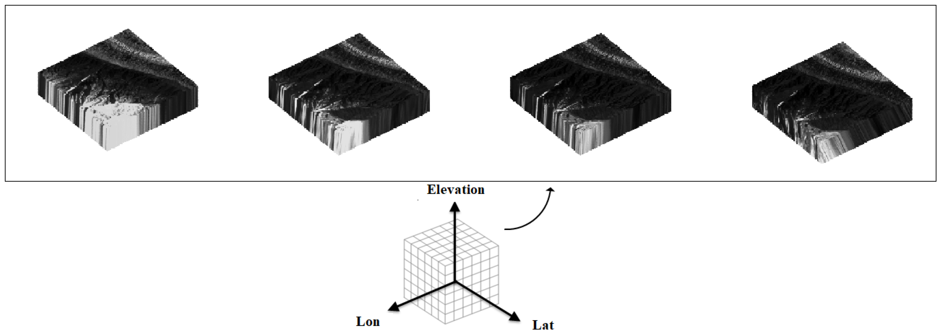
The ground coordinates of the four corners of each image are given in the metadata file of the image, which were used to select images covering the current tile of the AOI. Then, using RPC of each image, the image was projected on to the voxel space, thus creating a 3D volume for each image, as shown in Figure 1. Thus, for n images covering the spatial extent of the current tile of AOI, n image volumes were created. Now, the photo consistency measure could be applied to estimate the elevation at each grid point. Here, Census [41,42] was used as the local matching cost with a window size of $9\times 9$. Given n image volumes, there were $\frac{n(n-1)}{2}$ pairwise combinations on which Census matching and subsequently SGM could be applied. Thus, $\frac{n(n-1)}{2}$ matching costs were computed by first computing pairwise matching using Census and then optimizing the costs using eight path SGM. The cost function for SGM is:

$${\displaystyle E\left(Z\right)=\sum _{g}C(g,Z)+\sum _{f\in N_g}(P_{1}T\left[\right|Z_g-Z_f|=1])+\sum _{f\in N_g}(P_{2}T\left[\right|Z_g-Z_f|>1])}$$

(9)

where $C(g,Z)$ is the local matching cost at each grid point for different values of elevation (Z), $P_{1}T$ is the penalty for elevation difference of one voxel, $P_{2}T$ is the penalty for all elevation differences greater than one voxel and f is the grid point in the neighborhood ($Ng$) of g. This cost function can be optimized efficiently in 1D. In the SGM algorithm, this cost was optimized for 8 or 16 1D paths and the resulting cost was aggregated. The minimum cost location at each grid point gives the elevation. The sub voxel elevation values were computed by fitting a quadratic curve to the neighboring costs of the minimum cost location at each grid point. The final elevation was then computed by taking the median of pairwise elevations estimated at each grid point. A spatial median filter was then applied on the resulting elevations. The resulting point cloud with regular grid spacing may still contain errors or outliers, which are usually small segments of points located at a larger distance from the actual surface. These points were filtered out by computing the median distance of k-nearest neighbours for each point and the points which exceed a pre-defined threshold were removed. RPC refinement, dense matching and point cloud filtering were implemented in MATLAB.

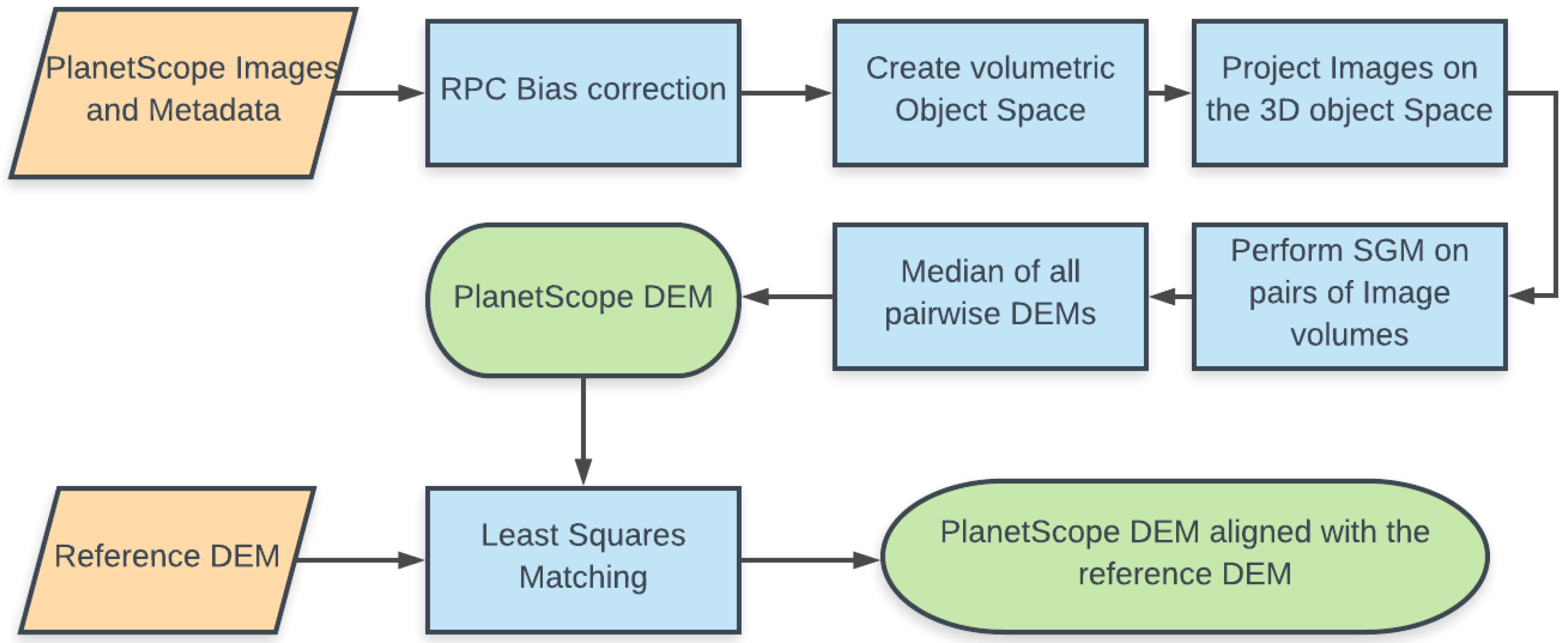
The filtered point cloud was transformed from Geographic coordinates to UTM coordinates for further processing. The filtered point was then interpolated into a raster of required grid size using a planar interpolation in which a plane was fitted to the neighbors of each grid point. To compare the computed DEM with other reference DEMs such as ALOS or LiDAR DEM, the two DEMs should be coregistered to each other. For this purpose, a Least Squares Matching (LSM) [43] approach was performed on the two DEMs to register them together. During the evaluation, it was observed that a shift in 3D was not sufficient for fine registration with the reference DEM. Therefore, a six parameter rigid transformation (3D rotation + 3D translation) was estimated and then applied to the PlanetScope DEM for fine registration. On test sites containing glaciers and snow, the glaciated regions were filtered out so that the LSM was only performed using the stable terrain. The outlines of the glaciated areas were extracted from Randolph Glacier Inventory (RGI) [44]. The rasterization of the point cloud and the LSM was performed using software OPALS [45]. The flow chart of the methodology is presented in Figure 2.

The B/H ratio is directly linked to quality of the DEM. As the B/H ratio decreases, the resulting elevation models get noisier. Therefore, pairwise matching is not performed for image pairs having B/H less than 1:60 as it was observed that results of lower B/H ratio image pairs were not reliable. The satellite position is not explicitly mentioned in the metadata of PlanetScope images. Therefore, the B/H ratio was calculated using RPC data by computing the image ray vectors for overlapping pixels of each image pair and computing the angle between these vectors. The convergence angle was then converted into B/H assuming a stereo normal case.

3. Study Areas

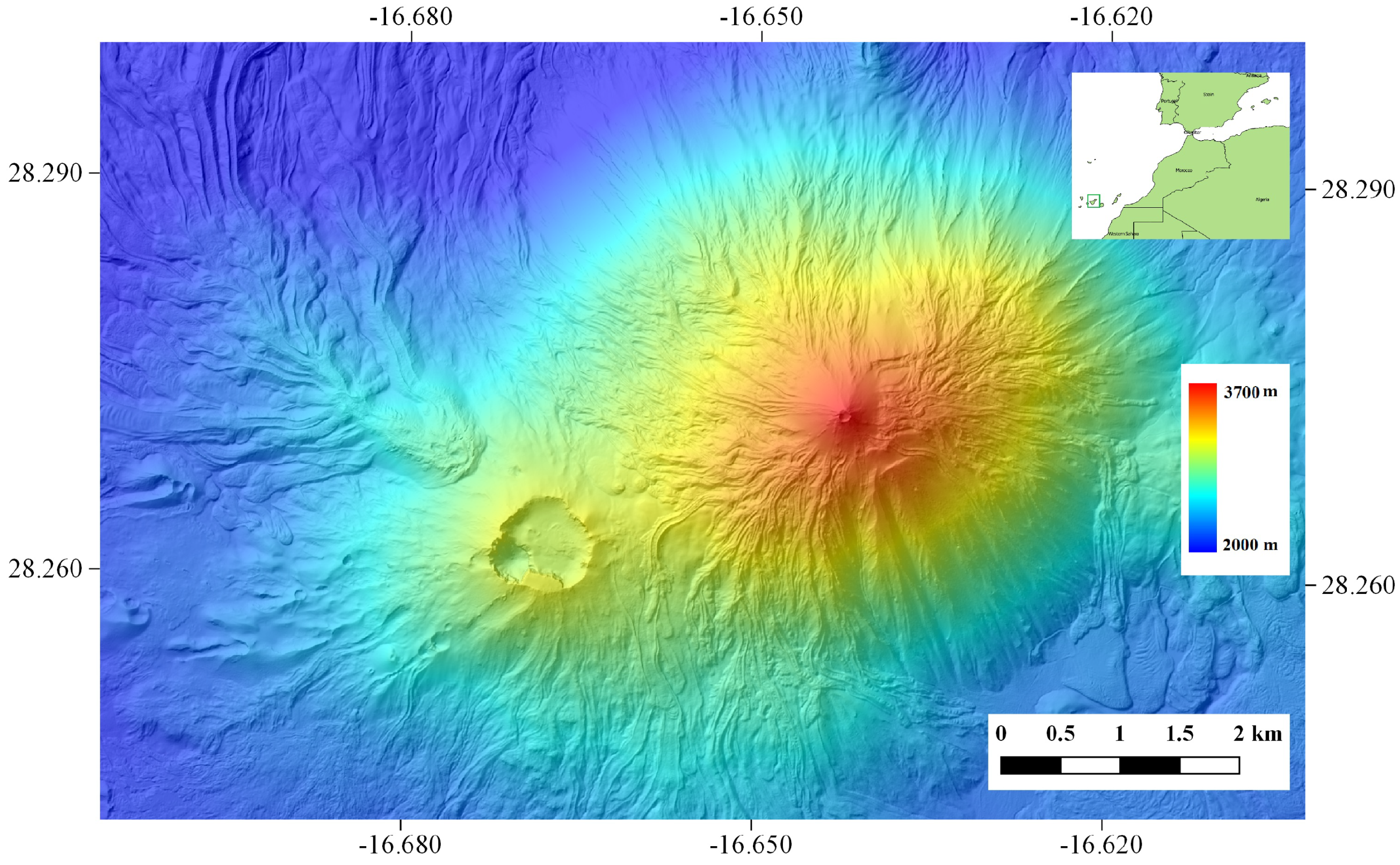
The first study area is Mount Teide (3718 m) in Tenerife, Canary Islands, Spain as shown in Figure 3. Mount Teide is an active volcano which last erupted in 1909. The subject area as shown in Figure 3 contains elevation range from 1800 m to 3718 m. This area was specifically chosen because of the availability of the LiDAR derived DEM and terrain similar to the high mountain ranges. The subject area contains minimal vegetation cover. The reference system of the LiDAR derived DTM as available from CNIG is REGCAN95 with UTM projection, while the elevations are orthometric according to the Earth Gravitational Model (EGM) 2008 fitted to the local vertical datum at the Canary Islands. The orthometric heights are converted to ellipsoidal heights by adding the geoid undulation to the orthometric height.

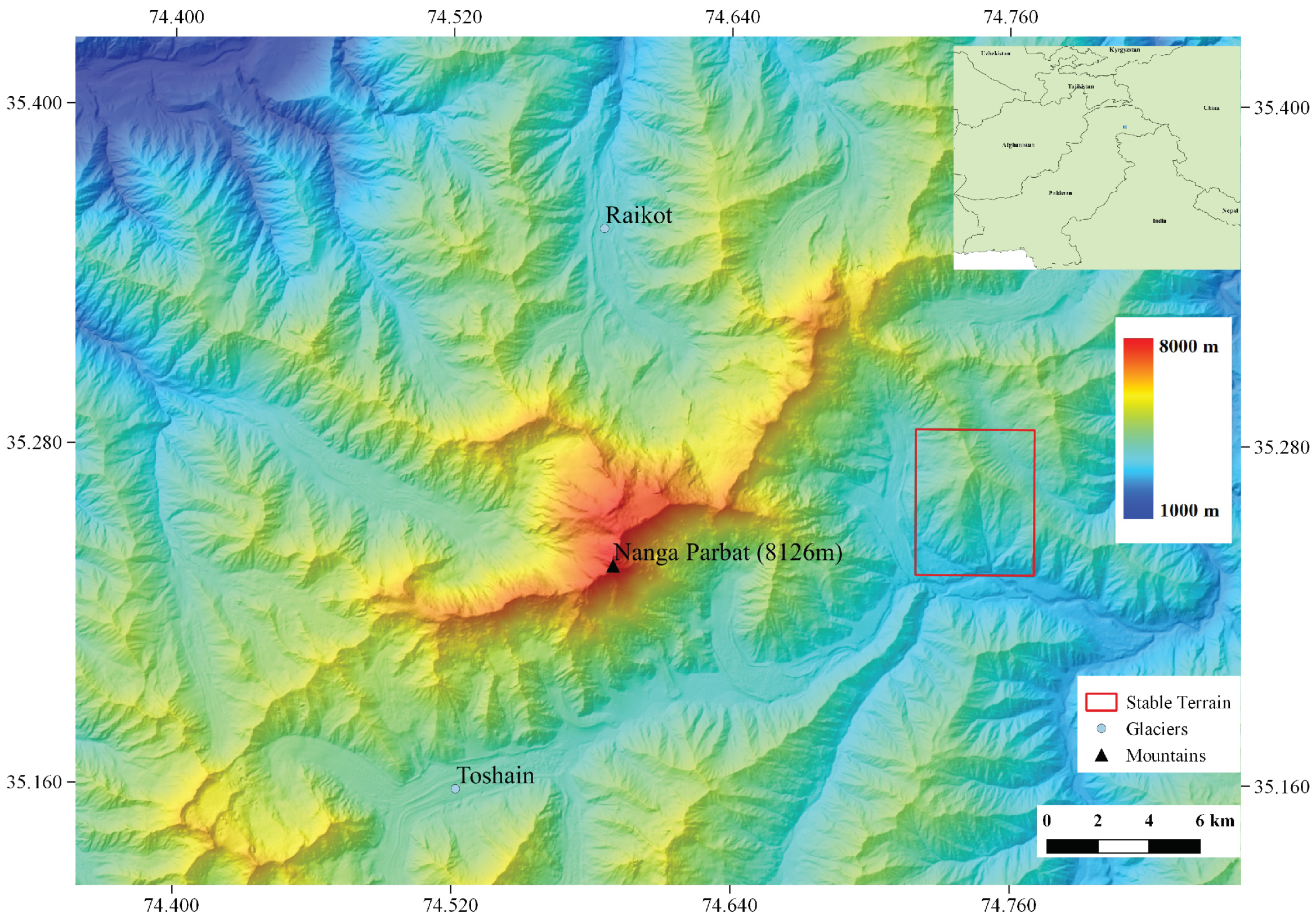
To test the vertical accuracy of the PlanetScope DEM on the rugged terrain of the Himalaya and Karakoram mountain ranges, the Nanga Parbat (8126 m) massif in the western Himalaya was chosen, which is the ninth highest peak in the world. The region and the AOI is shown in Figure 4. The glaciers in the Nanga Parbat massif have shown relatively small retreat, which is in contrast to the glacial retreat in eastern Himalaya [46]. The Nanga Parbat peak offers steep vertical relief over various locations and is therefore, a suitable site for evaluation of the methodology especially in the context of the glaciated high mountain ranges. Other high peaks in the region could also be chosen for such study. The most cloud free days in this region are in late autumn (October/November) but at this time of the year the Sun elevation is considerably lower which leads to large shadows that cause problems in image matching. Therefore, the choice of area depends on the availability of cloud free data with fewer shadows. Furthermore, in comparison to peaks such as K2 (8611 m), Nanga Parbat offers stable terrain (non-glaciated) in close proximity, which is required for fine registration of the PlanetScope DEM with a reference DEM. For the Nanga Parbat test area, ALOS DEM was used as the reference DEM. In ALOS DEM, the horizontal coordinates are according to the Geodetic Reference System GRS80, while the elevations are referenced to the EGM96 geoid, which are converted to the ellipsoidal heights for computing the elevation differences.

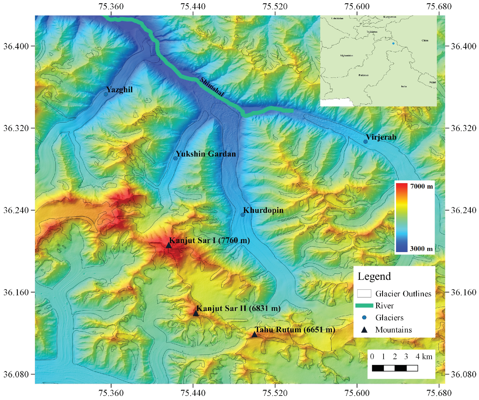
Now, to test the methodology over a dynamic scene, the Khurdopin Glacier (Figure 5) in the Shimshal valley of the Karakoram range was chosen. The glacier originates from the Tahum Rutum (6651 m), Kanjut Sar I (7760 m) and Kanjut Sar II (6831 m) peaks and the terminus of the glacier lies at the elevation of around 3400 m. The Khurdopin Glacier is especially significant due to its recent surge in 2017 with peak velocities of up to 5 km year${}^{-1}$ [47,48,49]. This glacier surge caused the blockade of the Shimshal River, which resulted in the creation of an ice dammed lake. During late July, the lake water drained from a subglacial stream. A sudden breach of such an ice dammed lake could cause floods and damage to the downstream settlements. The Khurdopin Glacier has surged in the past with a surging frequency of about 20 years. Several glaciers in this region have shown surging behaviour [50]. A better understanding of this surging activity is required especially due to the risks pertaining to the downstream settlements as well as the risks to the infrastructure.

4. Results

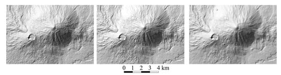
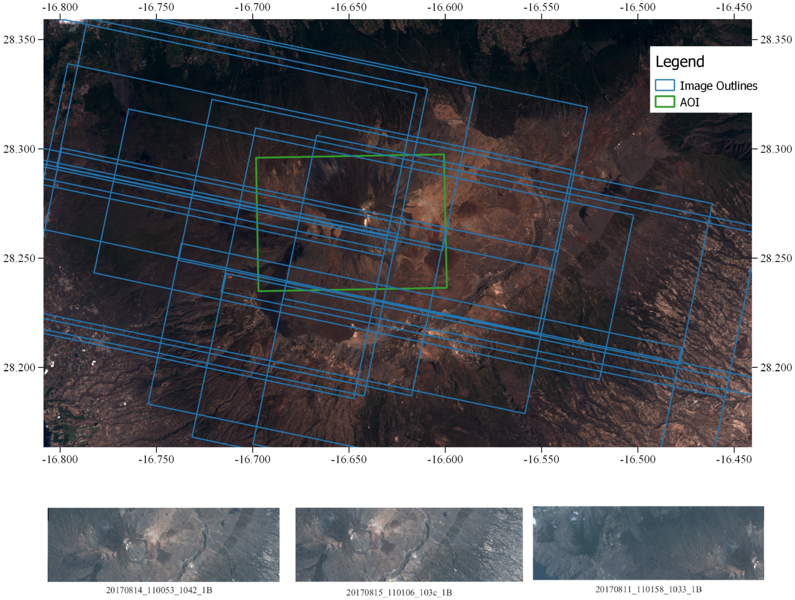
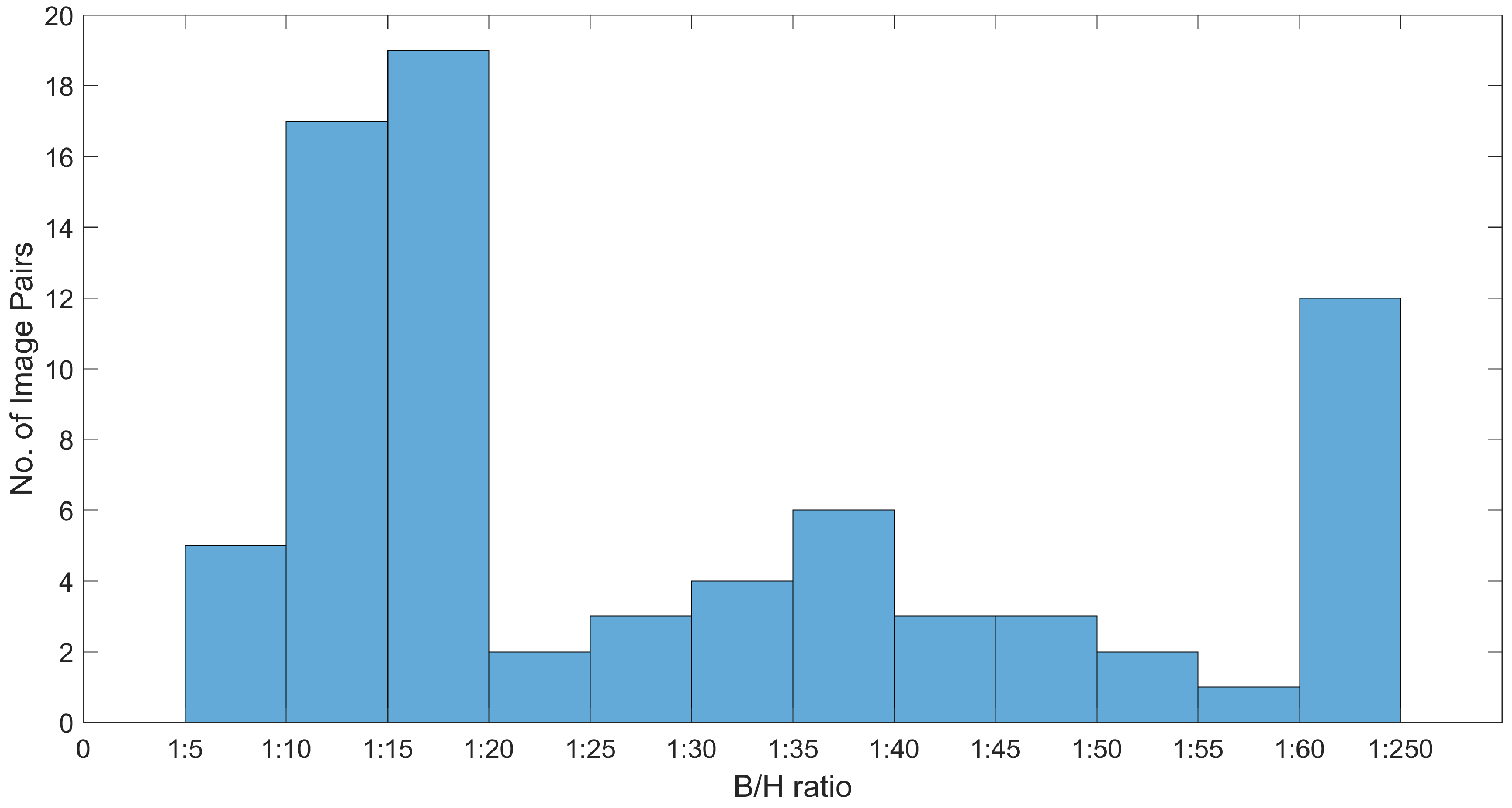
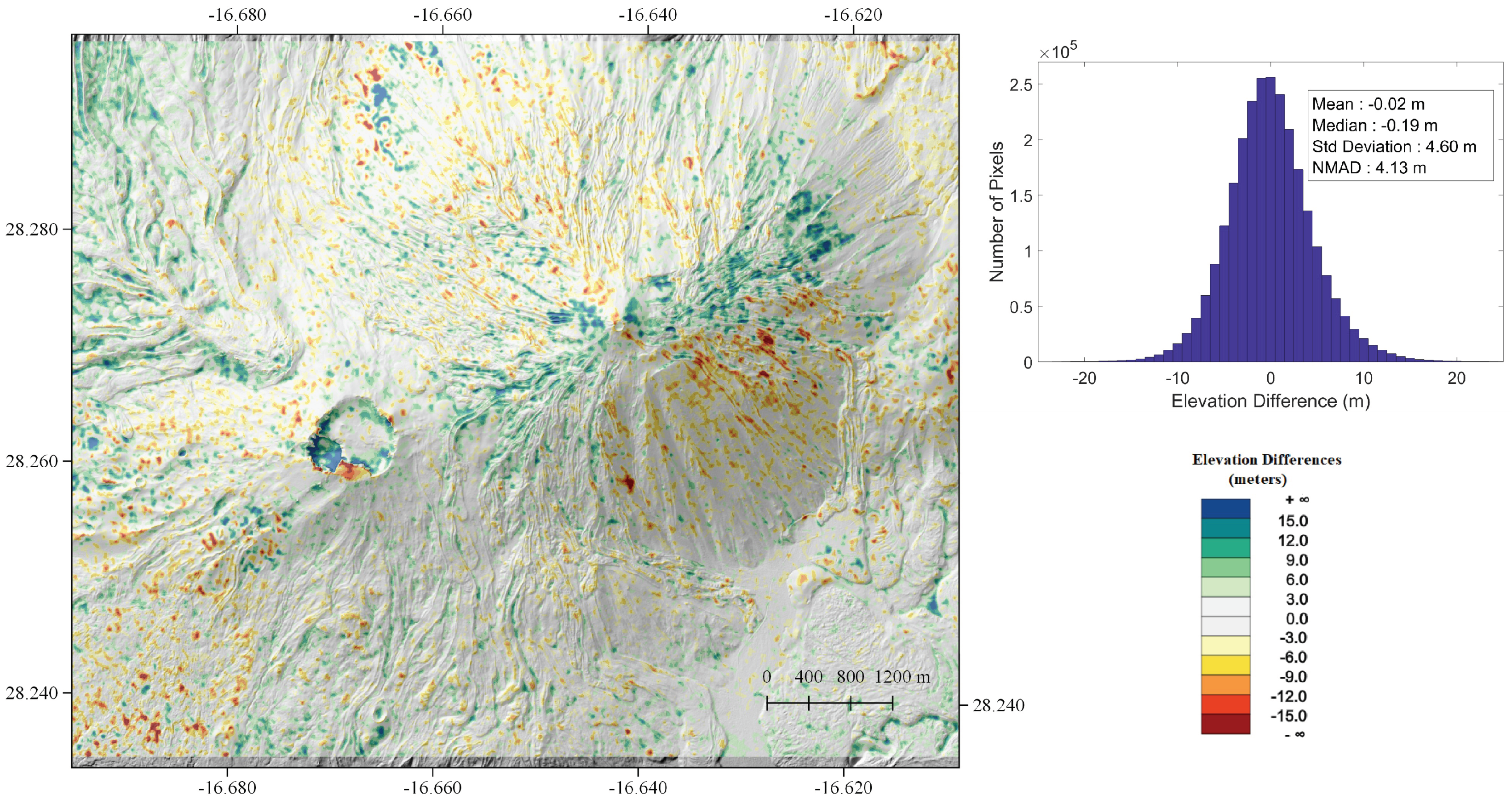
To create DEM of Mount Teide, PlanetScope image acquisitions from nine overpasses between 6 August 2017 and 30 August 2017 at around 11:00:00 UTC ± 5 min were used, as shown in Figure 6. The B/H ratio of the overlapping images are given in the histogram shown in Figure 7. The DEM was generated with a spatial resolution of 5 m covering an area of around 56 km${}^2$. The resolution of the DEM should in principle follow the Nyquist–Shannon criterion, i.e., the DEM resolution should be twice the GSD of images. For evaluation, the LiDAR based DEM with 5 m resolution is available, therefore, a 5 m DEM was created from PlanetScope imagery so that resampling of the reference LiDAR DEM is avoided. The elevation differences over the subject area are shown in Figure 8. The statistics of the elevation differences show that the two DEM are well registered and the NMAD is 4.1 m. 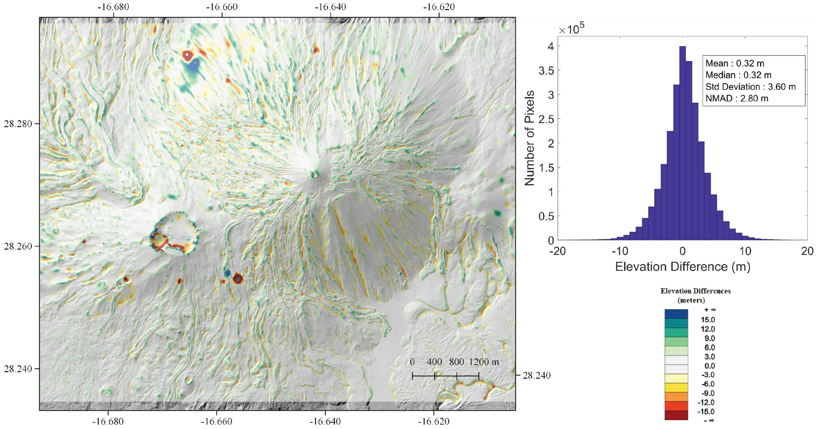The NMAD is a robust estimator of the standard deviation in the case of outliers in the data [51,52]. As a comparison, the NMAD of elevation differences between the LiDAR DEM and the ALOS (30 m) DEM over the subject area is 2.8 m, as shown in Figure 9. The ALOS 30 m DEM was resampled at 5 m resolution to compute the elevation difference between LiDAR and ALOS DEM as the 5 m ALOS DEM was not available. 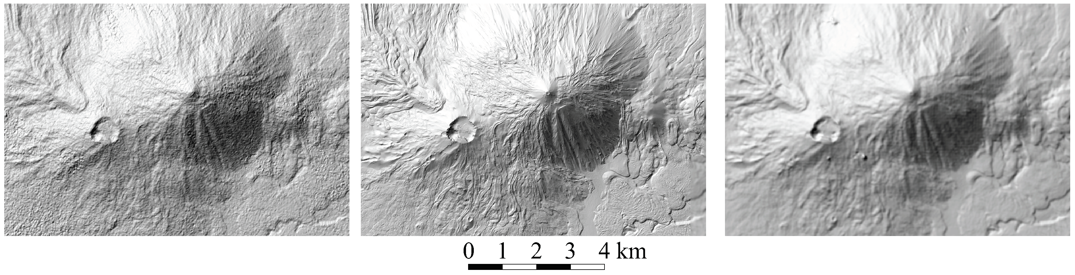Figure 10 shows the hillshades of the PlanetScope, LiDAR and ALOS DEMs. The visual analysis of the Hillshades also show that the PlanetScope DEM captures a similar level of detail as the ALOS DEM, however the PlanetScope DEM contains much higher noise.

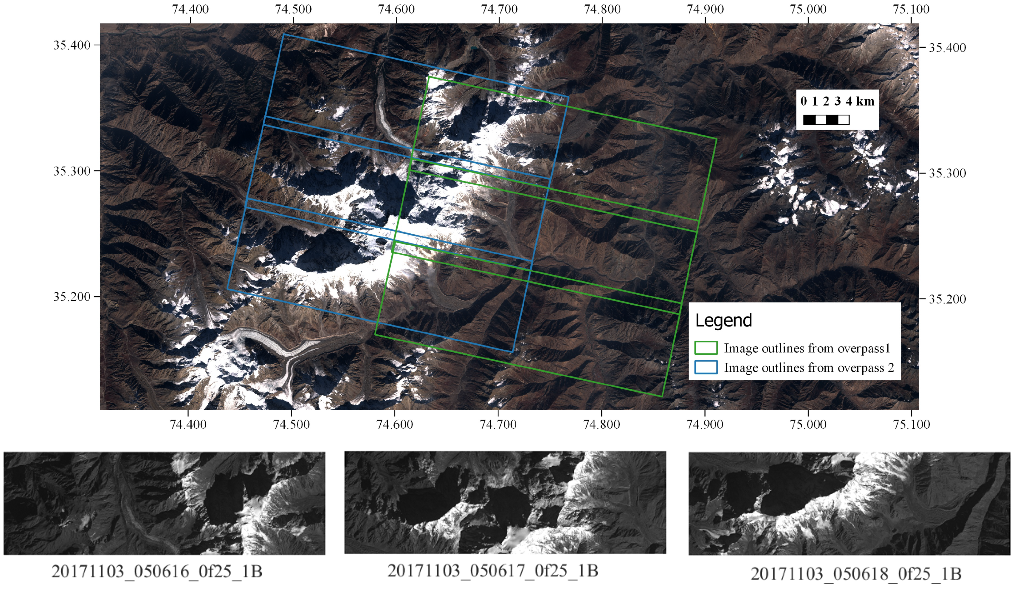
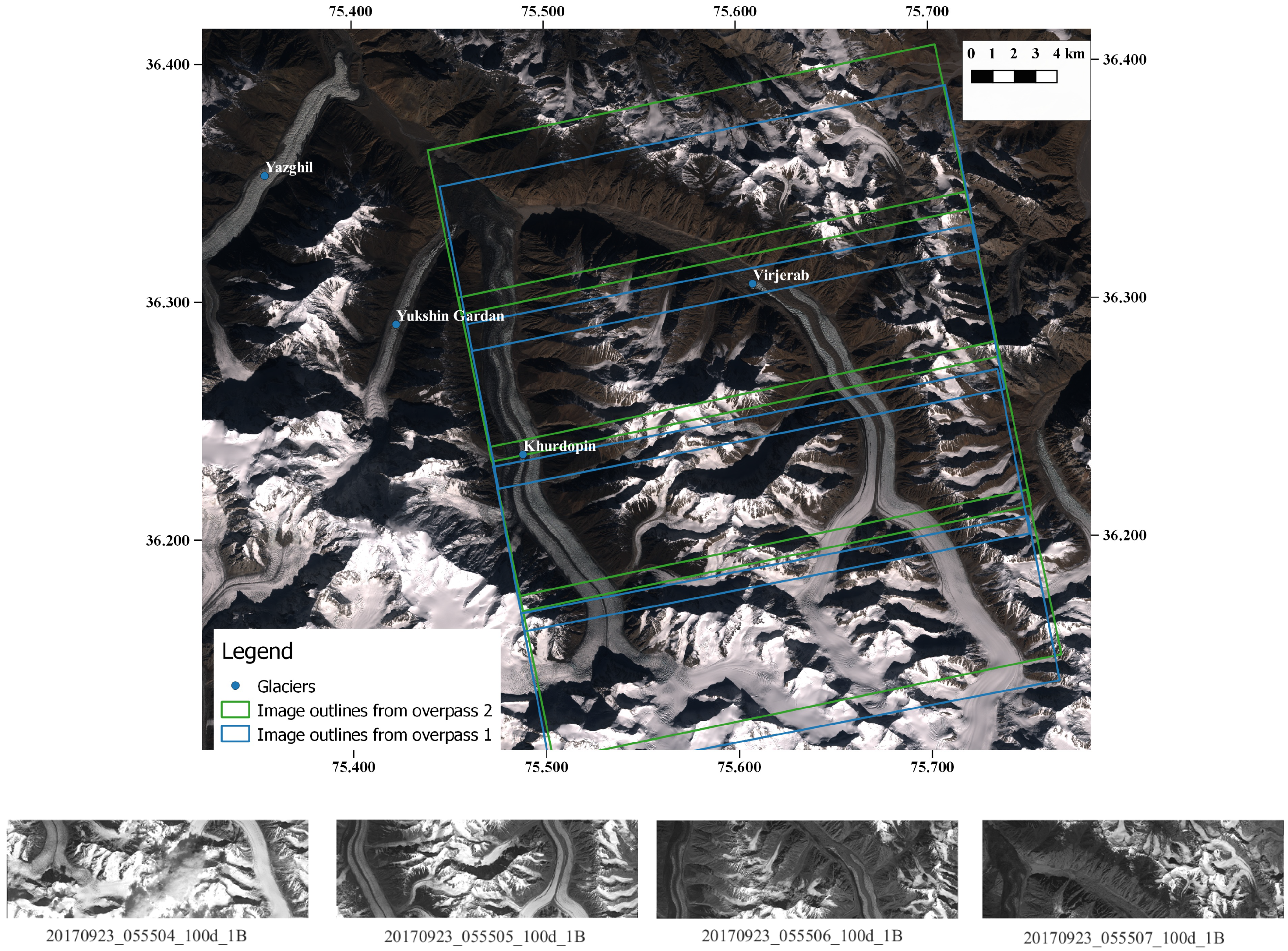
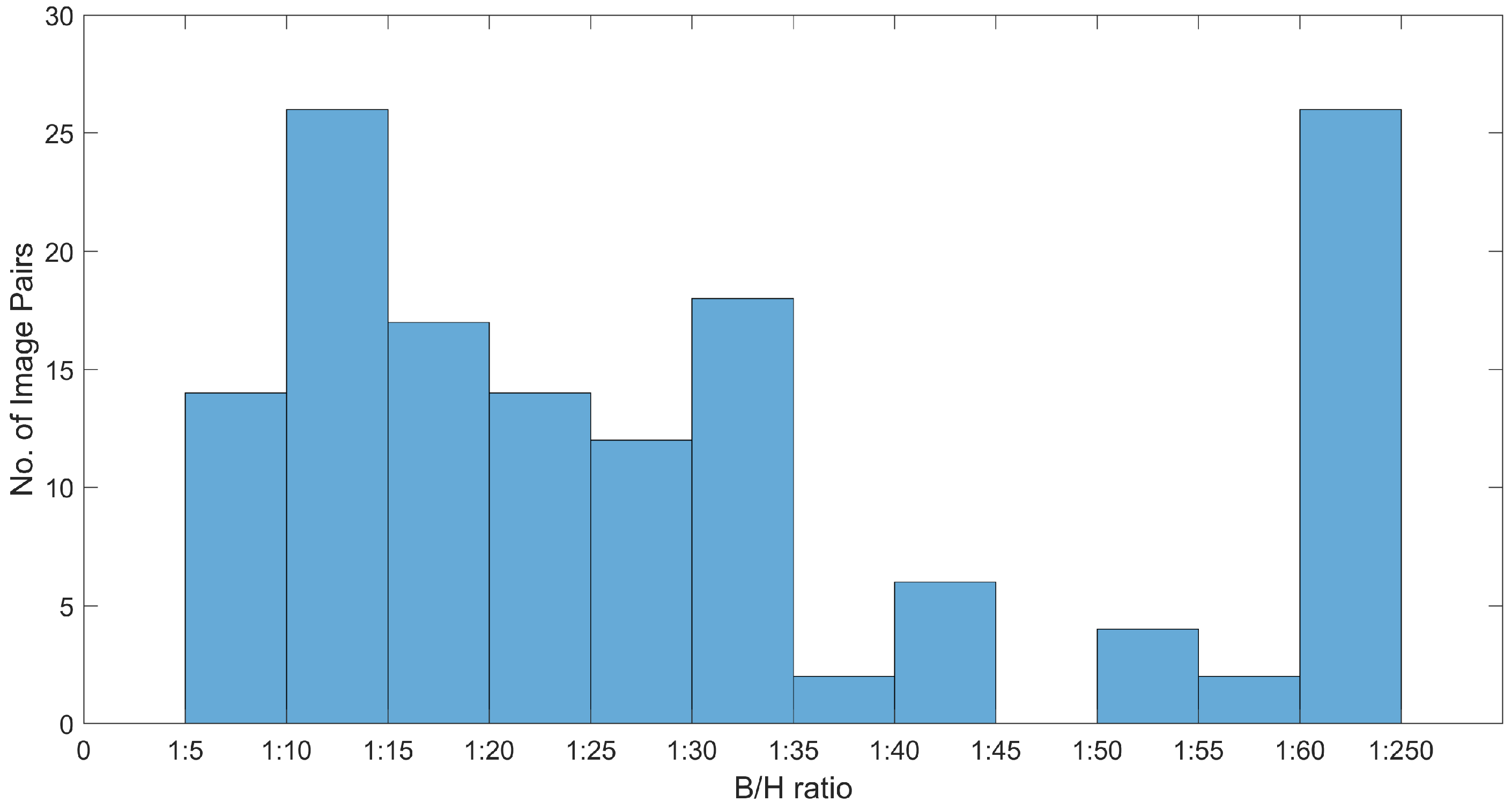
The DEM generation process is then evaluated on the Nanga Parbat massif in the Western Himalaya. The DEM generation was done on an area of about 324 km${}^2$ using thirty Plantscope images acquired between 30 October 2017 and 7 November 2017 at around 05:04:00 UTC ± 3 min from 14 overpasses over the subject area. Figure 11 shows the outlines of six images from two overpasses and the individual images from single overapass. 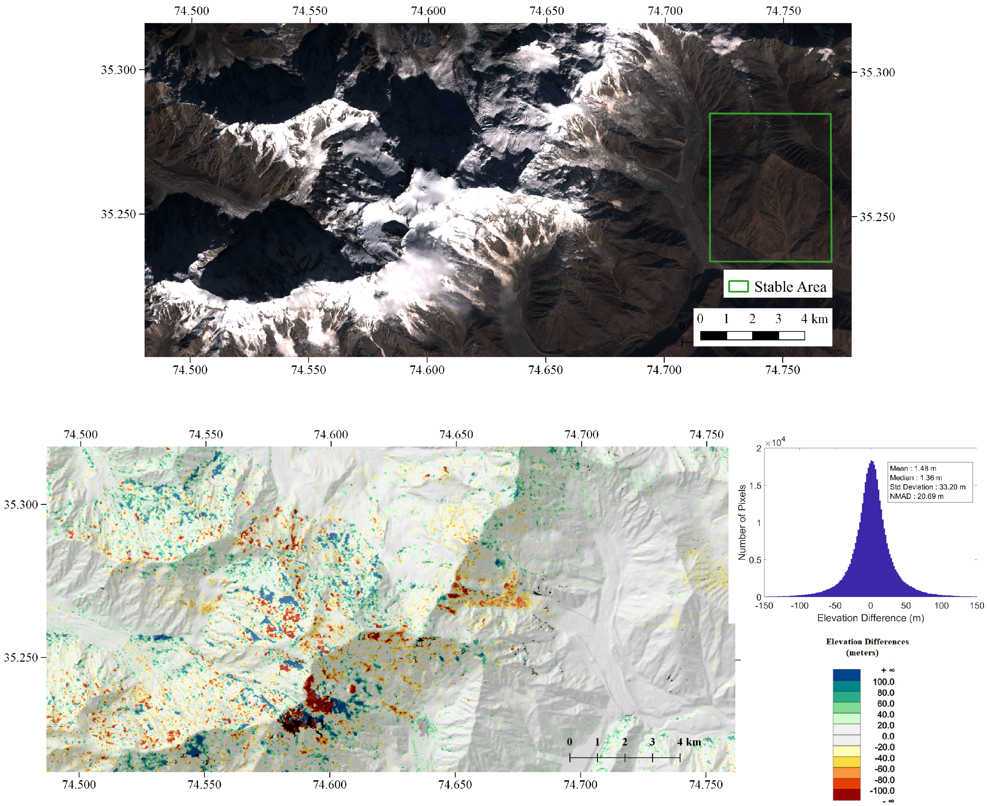The B/H ratio of the overlapping image pairs are given in the histogram shown in Figure 12. Large number of pixels in Red, Green and Blue bands are saturated in the subject area. On the other hand, very little texture is visible in the shadows in the NIR band. Therefore, the DEM is generated by taking of the median of the elevation maps from Red and NIR bands. The elevation differences between the PlanetScope DEM and the ALOS DEM are shown in Figure 13. The histogram shows the statistics of the elevation differences between the two DEMs. The median error is 1.36 m and normalized median absolute deviation (NMAD) is 20.69 m. It should be noted that the major part of this area is snow covered or glaciated and most of the outliers visible in Figure 13 belong to the snow covered area. The elevation differences over the snow covered area can actually be because of the change in the surface elevation due to snow accumulation or snow melting during the large time differences between the data acquisition of the two DEMs. Therefore, it is recommended to compare elevation differences over supposedly stable parts of the AOI, i.e., non-snow/ice covered areas. 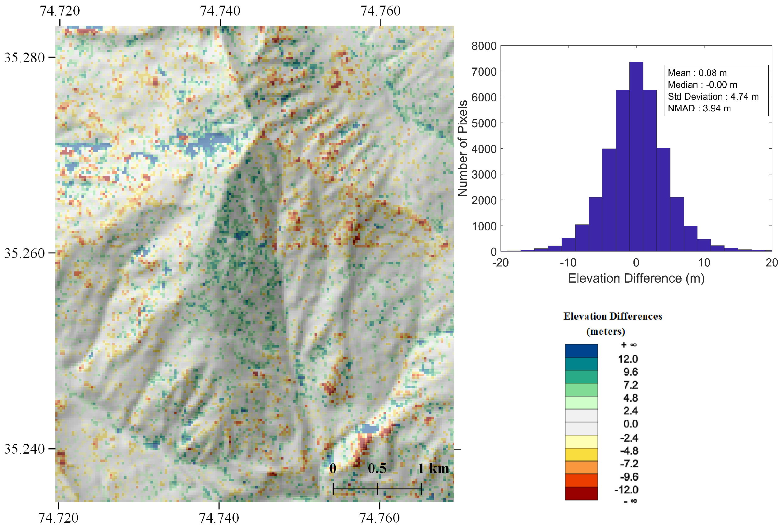For this purpose, DEM was again computed for an area of about 25 km${}^2$ on the east side of the Nanga Parbat, as shown in Figure 14. The area contains minimal shadows as well as no snow cover. The elevation range is from 2600 m to 4600 m, while the maximum slope is $58.2$ degrees and a mean slope of $28.9$ degrees. The median elevation difference between the ALOS and the PlanetScope DEM is 0.00 m, while the NMAD over stable terrain is 3.9 m. It should be mentioned that both ALOS and Planetscope DEM are created from stereo/multi view images. Therefore, errors are expected in low texture areas and occluded pixels. A visual inspection of the elevation differences shows that most of the outliers occur in small shadowed areas. It has been observed that in shadowed regions the texture is not discernible as a result the image matching does not perform well over shadowed regions. Consequently, the elevations at the shadowed regions are biased towards higher elevation. This is visible in the elevation differences shown in Figure 13 and in the statistics of elevation differences, i.e., median elevation differences is biased towards a positive value.

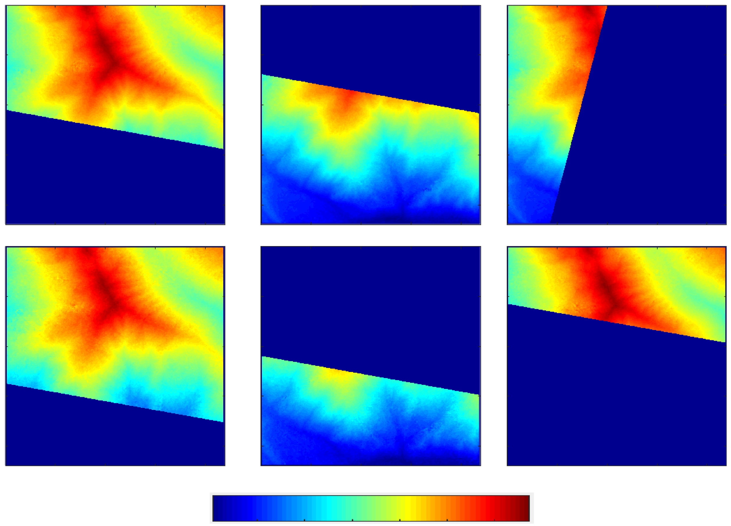
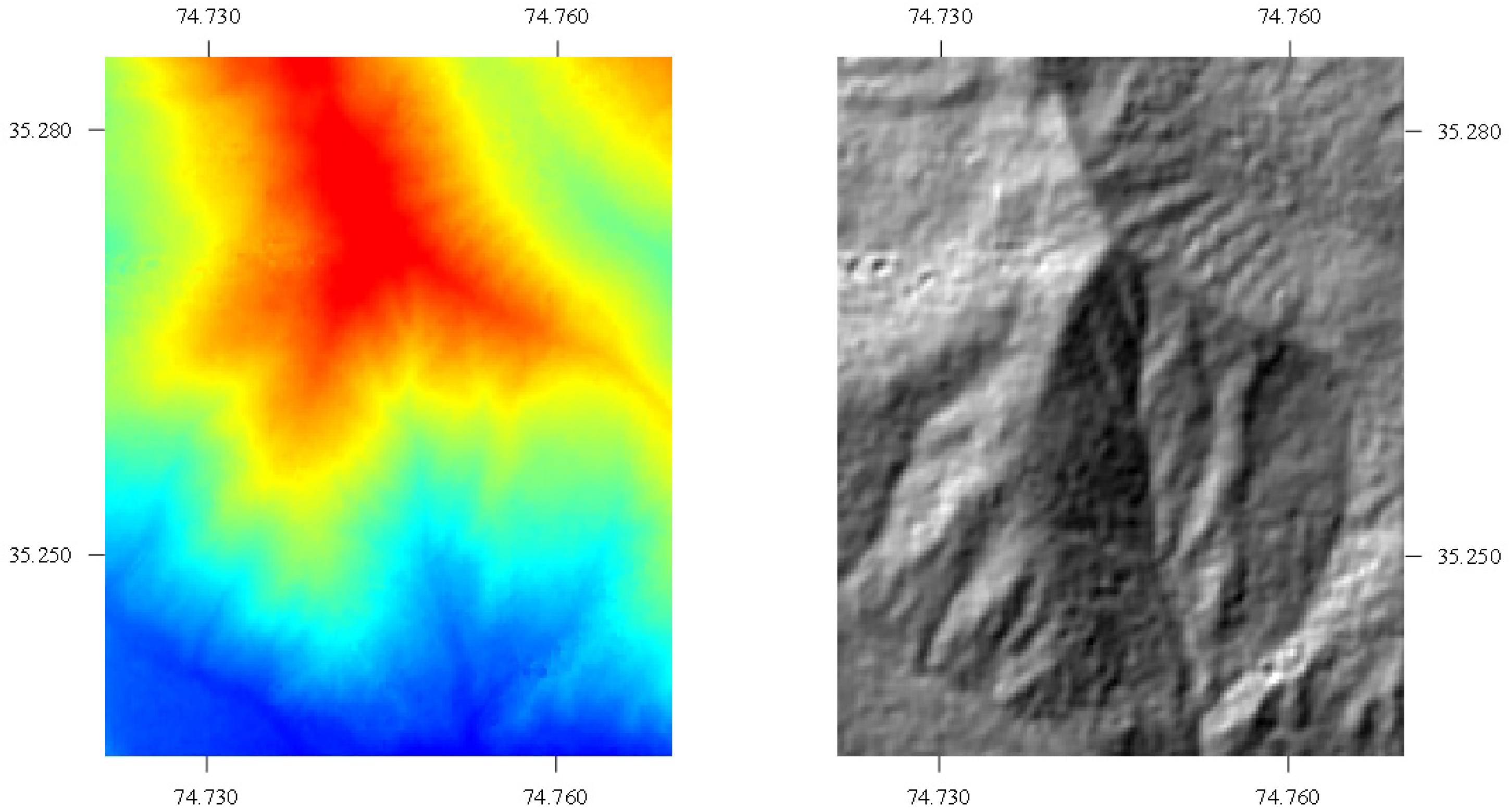
Figure 15 shows the results of SGM from pairwise matching of overlapping image pairs on the stable terrain of about 25 km${}^2$. As the individual images may only cover part of the AOI, the tile partly contains no data in the pairwise SGM. The final elevation model of the given tile is computed by taking median of the pairwise SGM results as discussed in previous section. The resulting DEM and the corresponding hillshaded model are shown in Figure 16.

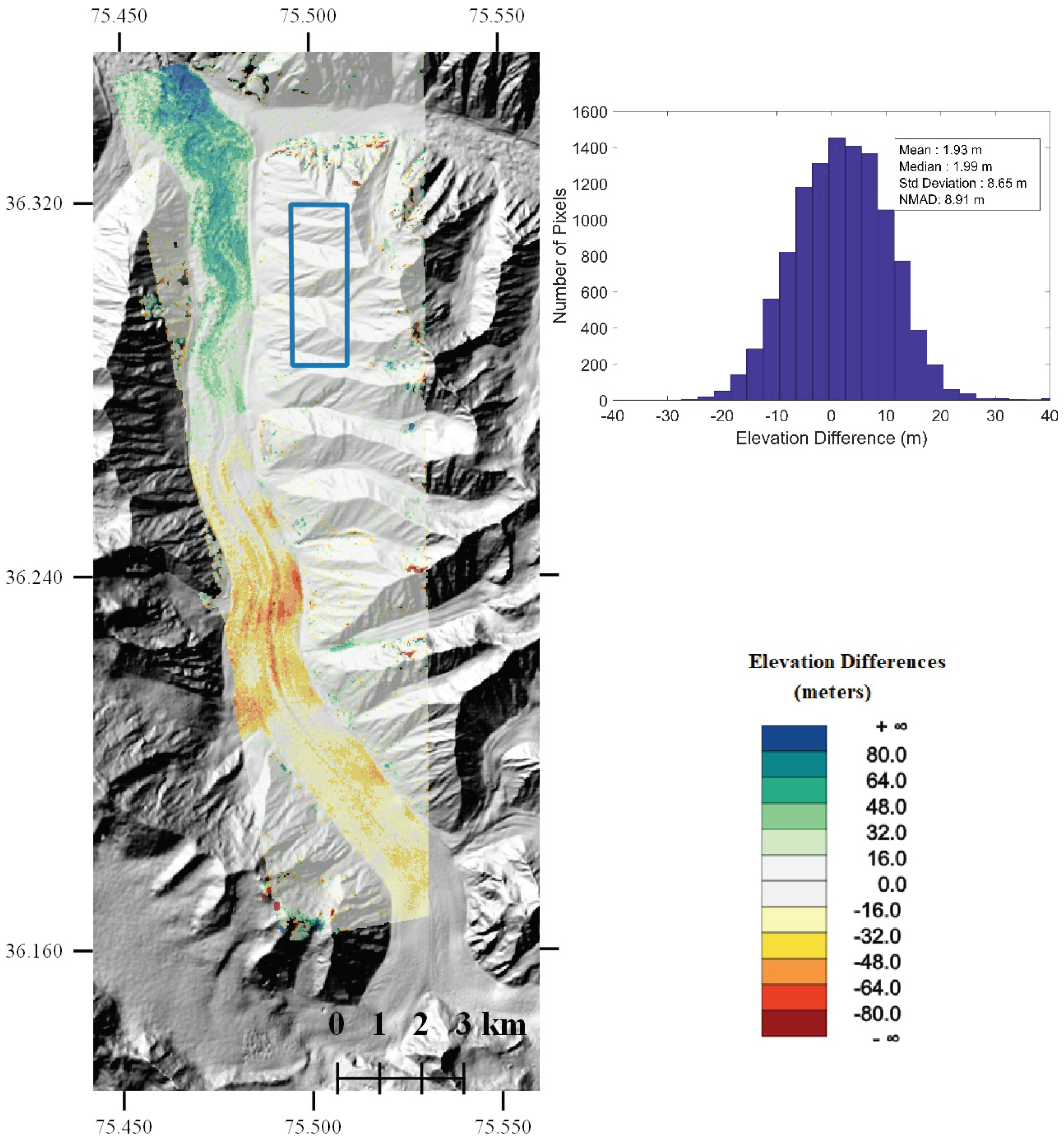
In the next test case, the elevation model over Khurdopin glacier was computed using PlanetScope images from two overpasses over the glacier from 23 September 2017, as shown in Figure 17. The glacier is in motion due to its recent surge, therefore, it is important to use images with a small time difference otherwise the motion of the glacier can lead to errors in the resulting DEM. The time difference between the two satellite passes is about 1.5 min. Three images from each overpass were taken to compute the DEM of the Khurdopin glacier. The images with the largest overlap have a B/H ratio of 1:13. The quality of the generated DEM was again evaluated using the stable terrain on the east side of the glacier. The statistics of the elevation differences over stable terrain shows that differences are greater than in the case of Nanga Parbat, which is due to the fact that images from only two overpasses were used to compute the DEM. Therefore, the quality of the DEM is lower due to low redundancy. The elevation differences over glacier, as shown in Figure 18, depict the changes in the glacier due to recent surge in which the volume of ice from the accumulation zone is transported downstream towards the valley. The validation of the elevation differences over glacier is difficult. An earlier study [48] has presented elevation differences over Khurdopin glacier using ASTER and TanDEM-X DEMs. In this study, ASTER DEM from May 2017 have been used to compute elevation difference due to glacier surge. Because the glacier is surging and there is a four-month time difference between PlanetScope DEM (September 2017) and the ASTER DEM (May 2017), the two DEMs cannot be directly compared.

The statistics of the elevation differences summarized in

Table 1. Summary of the area wise statistics of the elevation differences in meters (m). These statistics are calculated only for the stable terrain, as shown in the histograms above. $\sigma$ is the standard deviation. The approximate Sun elevation angle at the time of the image acquisitions for each test area are given in the 3rd column.

Area	Mean Slope (deg)	Sun Elevation (deg)	Mean	Median	$\mathit{\sigma }$	NMAD
Mount Teide	21.9	57	−0.02	−0.19	4.60	4.13
Nanga Parbat	28.9	33	0.08	0.00	4.74	3.94
Khurdopin Glacier	36.9	51	1.93	1.99	8.65	8.91

show that the results are promising in comparison to the earlier studies. In Tadono et al. [30], the standard deviation of elevation differences between the ALOS and SRTM DEMs of mountainous terrain in Nepal has been reported to be around 10 m. In Wong et al. [53], the standard deviation of elevation differences between SRTM (90 m) and a LiDAR derived DEM over mountainous tropical forest in Malaysia is reported to be around 10 m. In Hu et al. [32], the standard deviation of elevation differences between SRTM and DEM derived from aerial imagery has been reported to be around 18 m for a mountainous terrain in Hubei, China. 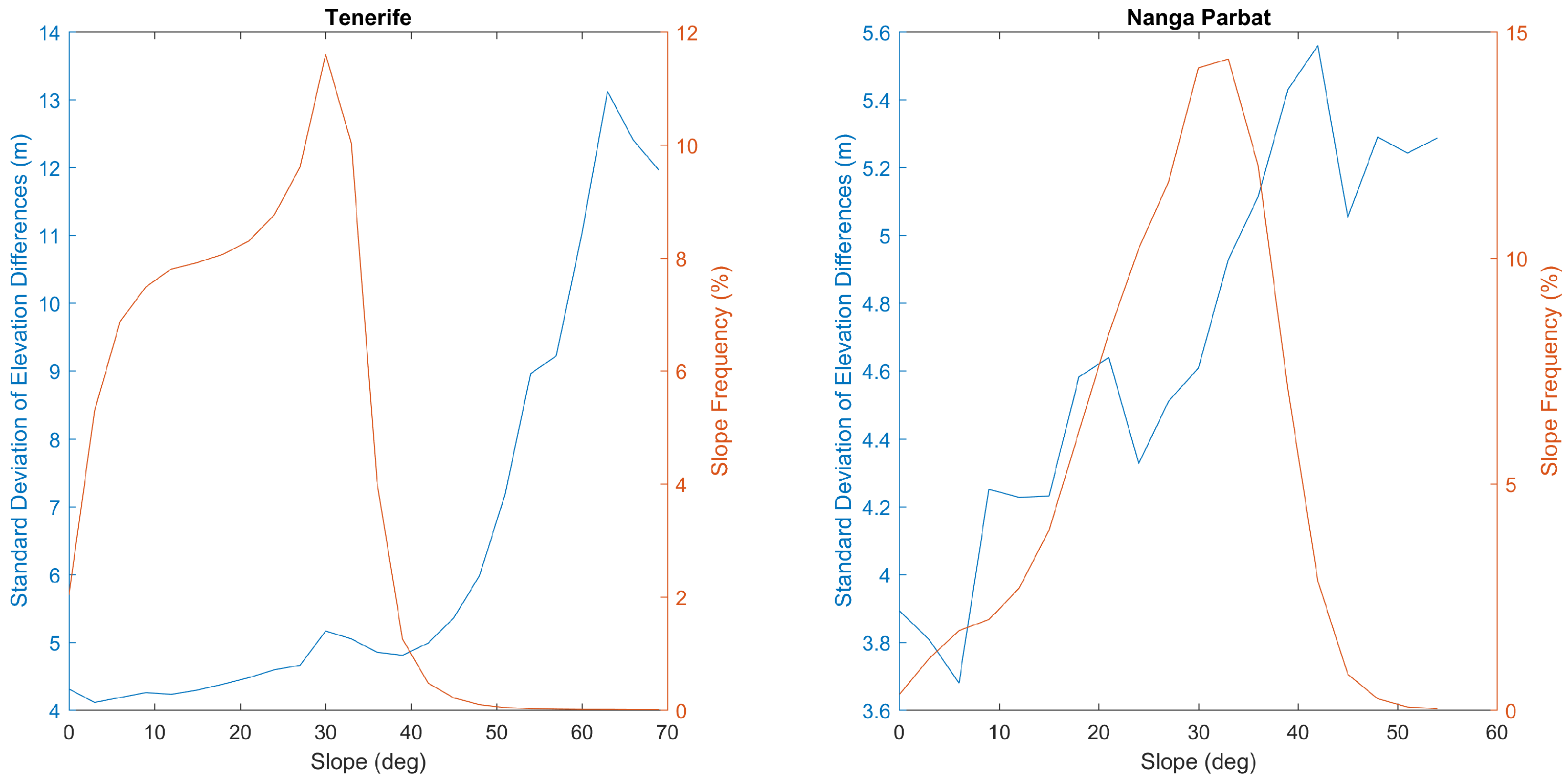In comparison, the summary of the statistics of the elevation differences of the three test areas used in this paper are shown in Table 1, which confirm the quality of the DEM generated from multiple PlanetScope Images. The variation in the elevation differences with different slope angles ($3^{\circ }$ bins) are shown in Figure 19. As expected, the standard deviation of the elevation differences increase with the slope of the DEM. However, the increase in the standard deviation is relatively smaller than the previous studies [32].

The results of the relative RPC bias adjustment using an affine model are given in

Table 2. Summary of the RPC refinement results. All values are in pixels. $\Delta x$ and $\Delta y$ are computed from Equations (5) and (6), respectively.

Area	Max $\Delta$x	Max $\Delta$y	Mean $\Delta$x	Mean $\Delta$y	RMSE
Mount Teide	0.46	0.36	0.07	0.09	0.16
Nanga Parbat	0.87	0.60	0.16	0.17	0.18
Khurdopin Glacier	0.44	0.27	0.07	0.05	0.16

. The results show that the RPC provided with the images are already accurate to within sub pixel range. However, the RPC refinement is still required, especially since the B/H is small, which results in a weak convergence angles. Even sub pixel RPC error can lead to large elevation differences in the resulting pairwise DEMs. The RMSE of the adjustment is around 0.17 pixels for all three test sites.

Table 3. Approximate Baseline to Height ratio of the image pairs used for each area. Last column shows the number of image pairs with B/H less than 1:60.

Area	Max B/H	Min B/H	B/H < 1:60
Mount Teide	1:7	1:57	12
Nanga Parbat	1:7	1:59	26
Khurdopin Glacier	1:13	1:13	0

gives the summary of the statistics of the B/H ratio of image pairs used for each area. The last column of Table 3 shows the number of image pairs whose B/H is less than 1:60. It should be noted that, even though some image pairs have B/H ratio better than 1:10, the overlap between them can be small. Therefore, it is important to utilize image pairs with smaller B/H for completeness as well as for increasing the redundancy.

5. Discussion

The accuracy of the derived DEM depends on the B/H ratio of the image pairs. As pointed out earlier, the B/H ratio of multisatellite PlanetScope imagery is typically small due to nadir looking configuration and a relatively smaller scene footprint. The better B/H ratio are the consequence of the off nadir view angle. Therefore, the potential of PlanetScope imagery for DEM generation is directly related to the image acquisition strategy of Planet. If the Dove constellation is operated in a strict nadir pointing mode (depending on the pointing accuracy of the Dove satellite’s attitude control system), then the B/H ratio will be small and subsequently the quality of DEM will be reduced as the smaller B/H ratio result in higher magnitude noise in the elevation models. Future advances in attitude control of small satellites could allow spacecraft operation at specific view angles, which could enhance the DEM generation potential of the PlanetScope imagery.

For static scenes, it is recommended to use images acquisitions from similar times of the day and preferably with only a few days difference, otherwise the movement of shadows (due to change in the Sun position in the sky) cause errors in the resulting DEM. For the Mount Teide test area, cloud free image acquisitions were not available on consecutive days. As a result, PlanetScope images from nine overpasses from 6 August 2017 to 30 August 2017 were used for Mount Teide test area. Decreasing the number of images decreases the redundancy and leads to larger elevation differences between the PlanetScope and the reference DEM. Therefore, utilizing images with relatively larger time difference in image acquisitions was unavoidable for the Mount Teide test area.

The DEM generated from a single day images of Khurdopin glacier is especially significant and can have far reaching implications in the context of studying dynamic phenomena. In the archives of PlanetScope daily imagery, a couple of other cloud free acquisitions over Khurdopin glacier from a single day are also available. 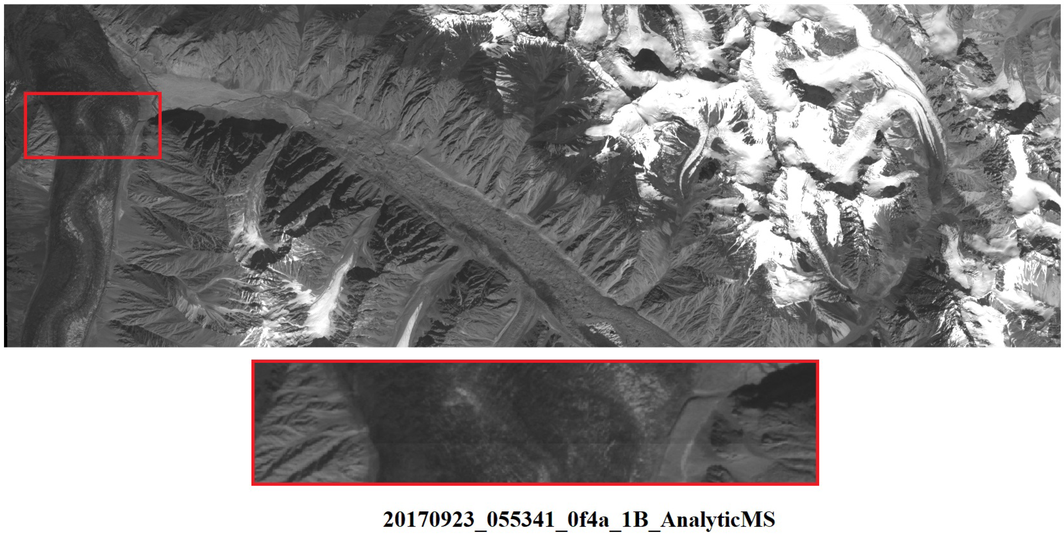The evaluation of those images has also revealed similar results as given in Figure 18. For some same day acquisitions, the B/H ratio is too small for generating reliable DEM. The registration of the Khurdopin Glacier DEM was challenging due to large snow covered area and large shadows due to high relief. Subsequently, the registration of the Khurdopin DEM is not as good as in the other two cases. The shadows in the image result in mismatches and eventually lead to inaccuracies in the DEM. Therefore, images from summer season with highest Sun elevation are expected to give better results. However, the cloud free coverage is limited during this season especially in the Karakoram region. Furthermore, part of snow/ice having high reflectivity results in the saturation of the pixels even in the NIR band. The PlanetScope imagery comes with an Unusable Data Mask (UDM) file, which contains the mask for anomalous pixels that can be used to mask out saturated pixels. The availability of the multiple images, i.e., greater than two, for a given area is essential for a robust DEM computation. When using only two images, significant outliers have been occasionally observed in the computed DEM due problems in image matching. Some artefacts in the original images have also been observed as shown in Figure 20. A visual inspection of different PlanetScope images shows differences in the radiometric appearance of the images from different satellites. Although the Census matching cost is robust against global radiometric differences, a better radiometric calibration is expected to yield better output [54].

The RPCs provided with the PlanetScope imagery have good relative accuracy and the relative RPC bias is typically less than $0.5$ pixels, as shown in Table 2. As mentioned earlier, the RPC provided with each image are already refined using tie points from reference imagery. However, this process is only performed for each strip independently. Therefore, the RPC refinement process given above is expected to yield better 3D reconstruction as different images from different satellites are simultaneously utilized in the adjustment procedure. However, due to relatively smaller overlaps of some images, it has been challenging to find enough well distributed tie points in each image, which can then be utilized in the RPC refinement process. This problem was especially significant for the images of Khurdopin Glacier and Nanga Parbat where parts of the images get saturated because of high reflection from snow covered areas. Therefore, a better RPC refinement process would involve either Ground Control Points (GCP) or points from reference imagery covering the extent of the AOI. Due to short baseline, the resulting 3D reconstruction is very sensitive to the RPC bias present in each image pair. If the bias correction is not performed correctly, then there are mismatches between the elevations computed from each pair. Some systematic errors in the elevation differences can be noticed in the results provided above. Therefore, a further evaluation of the RPC bias compensation in PlanetScope imagery is required.

6. Conclusions

This paper presents a methodology for creating DEM from multisatellite PlanetScope imagery. The results show that, even with a small baseline, multiple images from different overpasses can be utilized to create good quality DEM, which can be an alternative to freely available DEMs such as SRTM, ALOS and ASTER. The proposed methodology and results are especially significant for studying dynamic phenomenon as well as investigating the disaster related events such as avalanches or landslides because the pre and post event images are acquired daily by PlanetScope satellites (assuming cloud free coverage). The NMAD value of 4.1 m for the elevation differences between the LiDAR and PlanetScope DEM shows that the quality of the DEM is good in comparison to the earlier studies, which have compared global DEMs with GCPs and LiDAR data. The NMAD of elevation differences between ALOS and PlanetScope DEM on stable area around Nanga Parbat is 3.9 m. The good quality of the DEM can perhaps be attributed to the fact that image matching performs well with small baseline images along with the fact that multiple image pairs can be utilized for static scenes, which increases the redundancy and leads to better accuracy of the elevation models. Further improvements in the results is expected when using ground control points for RPC refinement, as well as performing a better denoising of the generated elevation models. The DEM generation potential of the PlanetScope imagery is however strongly linked to the data acquisition strategy by Planet. A more constrained nadir pointing can lead to smaller B/H ratio, which could adversely effect the DEM generation potential. On the other hand, operating Dove satellites at specific view angles could enhance the DEM generation potential of the PlanetScope imagery.