Mapping Inter-Annual Land Cover Variations Automatically Based on a Novel Sample Transfer Method


Abstract

1. Introduction
2. Materials
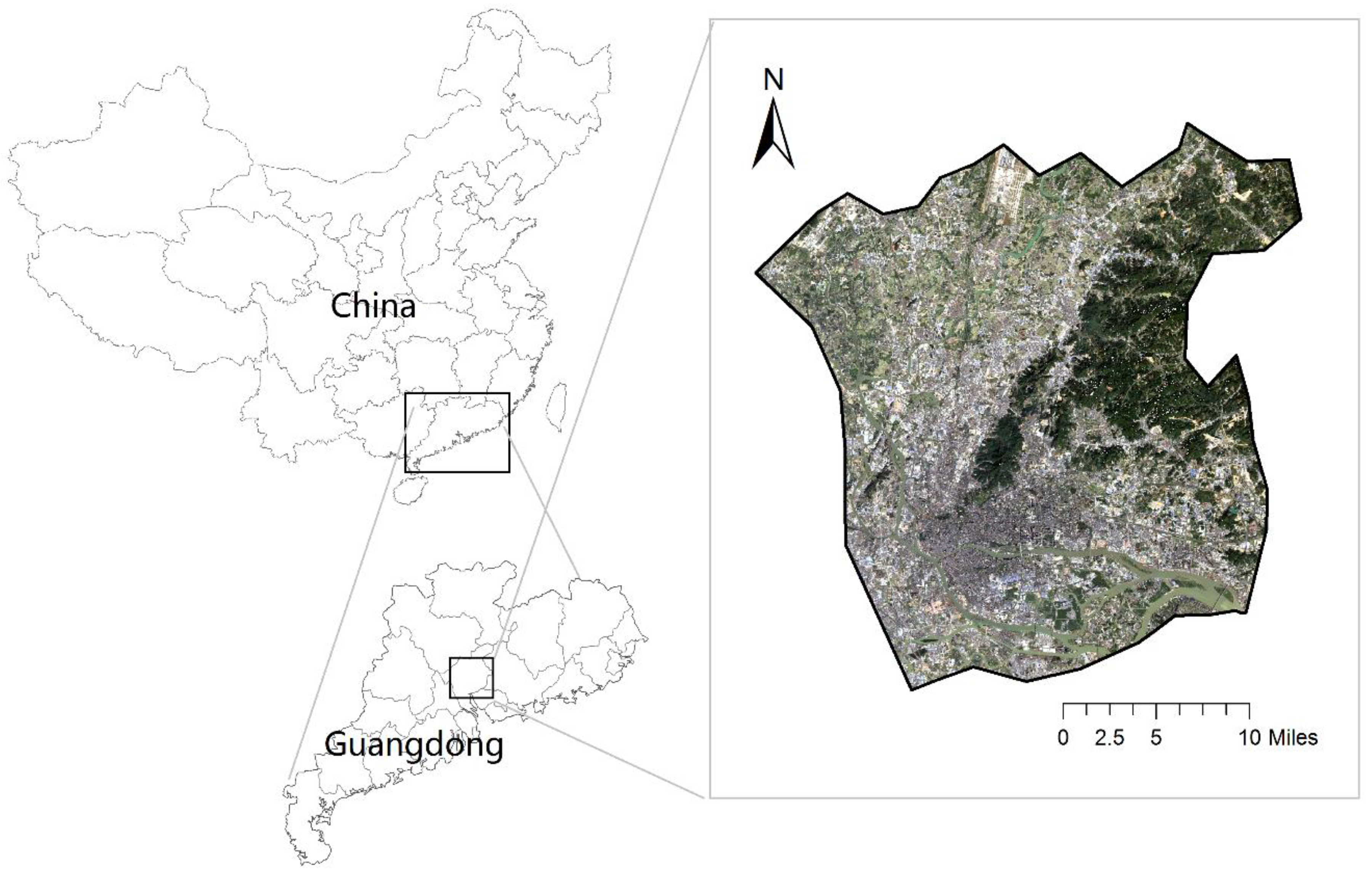
2.1. Study Site
2.2. Data
3. Methods
3.1. Image Segmentation
3.2. Feature Definition and Selection
3.3. Sample Selection
3.4. Sample’ Transfer
3.5. Classification and Performance Evaluation
4. Results
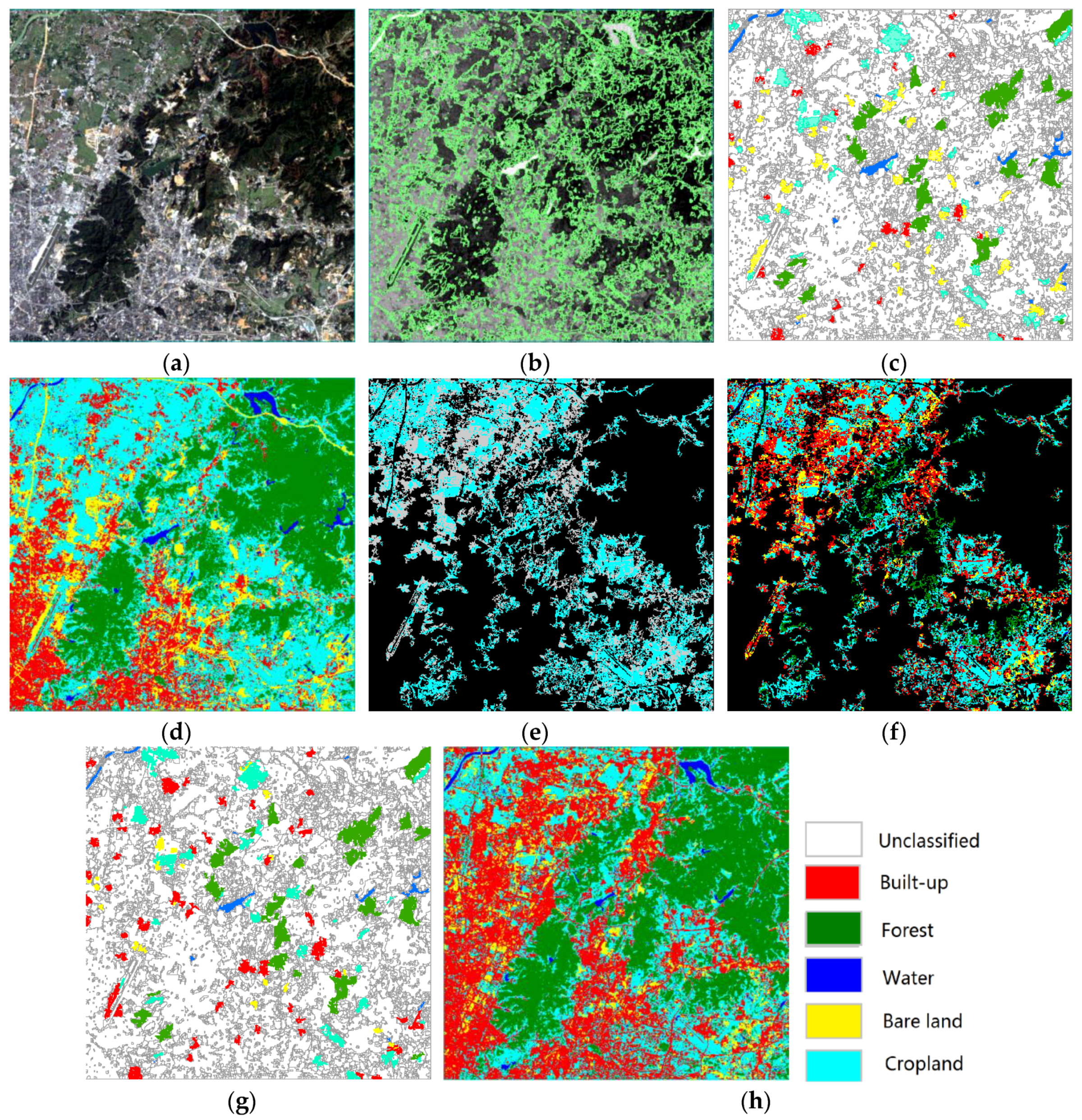
4.1. The Process of Presented Method
4.2. Validation and Comparison
4.3. Land Cover Dynamics of the Study Site
5. Discussion
5.1. Characteristics of the Proposed Method
5.2. Issues of Guangzhou Urbanization
6. Conclusions
Author Contributions
Funding
Acknowledgments
Conflicts of Interest
References
- Su, S.; Xiao, R.; Jiang, Z.; Zhang, Y. Characterizing landscape pattern and ecosystem service value changes for urbanization impacts at an eco-regional scale. Appl. Geogr. 2012, 34, 295–305. [Google Scholar] [CrossRef]
- Dewan, A.M.; Yamaguchi, Y. Land use and land cover change in Greater Dhaka, Bangladesh: Using remote sensing to promote sustainable urbanization. Appl. Geogr. 2009, 29, 390–401. [Google Scholar] [CrossRef]
- Guan, D.; Li, H.; Inohae, T.; Su, W.; Nagaie, T.; Hokao, K. Modeling urban land use change by the integration of cellular automaton and Markov model. Ecol. Model. 2011, 222, 3761–3772. [Google Scholar] [CrossRef]
- Kontgis, C.; Schneider, A.; Fox, J.; Saksena, S.; Spencer, H.J.; Castrence, M. Monitoring peri-urbanization in the greater Ho Chi Minh City metropolitan area. Appl. Geogr. 2014, 53, 377–388. [Google Scholar] [CrossRef]
- Dewan, A.M.; Yamaguchi, Y.; Rahman, M. Dynamics of land use/cover changes and the analysis of landscape fragmentation in Dhaka Metropolitan Bangladesh. GeoJournal 2012, 77, 315–330. [Google Scholar] [CrossRef]
- Moghadam, H.S.; Helbich, M. Spatiotemporal urbanization processes in the megacity of Mumbai, India: A Markov chains-cellular automata urban growth model. Appl. Geogr. 2013, 40, 140–149. [Google Scholar] [CrossRef]
- Dewan, A.M.; Kabir, M.H.; Nahar, K.; Rahman, M.Z. Urbanisation and environmental degradation in Dhaka Metropolitan Area of Bangladesh. Int. J. Environ. Sustain. Dev. 2012, 11, 118–147. [Google Scholar] [CrossRef]
- Li, X.; Zhou, W.; Ouyang, Z. Forty years of urban expansion in Beijing: What is the relative importance of physical, socioeconomic and neighborhood factors? Appl. Geogr. 2013, 38, 1–10. [Google Scholar] [CrossRef]
- Byomkesh, T.; Nakagoshi, N.; Dewan, A.M. Urbanization and green space dynamics in Greater Dhaka Bangladesh. Landsc. Ecol. Eng. 2012, 8, 45–58. [Google Scholar] [CrossRef]
- Trotter, L.; Dewan, A.; Robinson, T. Effects of rapid urbanisation on the urban thermal environment between 1990 and 2011 in Dhaka Megacity, Bangladesh. AIMS Environ. Sci. 2017, 4, 145–167. [Google Scholar] [CrossRef]
- Xiao, L.; Yang, X.; Cai, H.; Zhang, D. Cultivated Land Changes and Agricultural Potential Productivity in Mainland China. Sustainability 2015, 7, 11893–11908. [Google Scholar] [CrossRef]
- Ma, Y.; Wu, H.P.; Wang, L.Z.; Huang, B.M.; Ranjan, R.; Zomaya, A.; Jie, W. Remote sensing big data computing: Challenges and opportunities. Future Gener. Comput. Syst. 2015, 51, 47–60. [Google Scholar] [CrossRef]
- Adjorlolo, C.; Mutanga, O.; Cho, M.A.; Ismail, R. Challenges and opportunities in the use of remote sensing for C3 and C4 grass species discrimination and mapping. Afr. J. Range For. Sci. 2012, 5490, 563–573. [Google Scholar]
- Aghakouchak, A.; Farahmand, A.; Melton, F.S.; Teixeira, J.; Anderson, M.C.; Wardlow, B.D.; Hain, C.R. Remote sensing of drought: Progress, challenges and opportunities. Rev. Geophys. 2015, 53, 452–480. [Google Scholar] [CrossRef]
- Carreiras, J.M.B.; Jones, J.; Lucas, R.M.; Gabrie, C. Land Use and Land Cover Change dynamics across the Brazilian Amazon: Insights from Extensive Time-Series Analysis of Remote Sensing Data. PLoS ONE 2014, 9, e104144. [Google Scholar] [CrossRef] [PubMed]
- Bey, A.; Díaz, A.S.; Maniatis, D.; Marchi, G.; Mollicone, D.; Ricci, S.; Bastin, J.; Moore, R.; Federici, S.; Rezende, M.; et al. Collect Earth: Land Use and Land Cover Assessment through Augmented Visual Interpretation. Remote Sens. 2016, 8, 807. [Google Scholar] [CrossRef]
- Hai, M.P.; Yamaguchi, Y. Urban growth and change analysis using remote sensing and spatial metrics from 1975 to 2003 for Hanoi, Vietnam. Int. J. Remote Sens. 2011, 32, 1901–1915. [Google Scholar]
- Rodriguez-Galiano, V.F.; Chica-Olmo, M.; Abarca-Hernandez, F.; Atkinson, P.M.; Jeganathan, C. Random Forest classification of Mediterranean land cover using multi-seasonal imagery and multi-seasonal texture. Remote Sens. Environ. 2012, 121, 93–107. [Google Scholar] [CrossRef]
- Botkin, D.B.; Estes, J.E.; Macdonald, R.B.; Wilson, M.V. Studying the earth’s vegetation from space. Bioscience 1984, 34, 508–514. [Google Scholar] [CrossRef]
- Thenkabail, P.S.; Biradar, C.M.; Noojipady, P.; Dheeravath, V.; Li, Y.; Velpuri, M.; Gumma, M.; Gangalakunta, O.R.P.; Turral, H.; Cai, X.; et al. Global irrigated area map (GIAM), derived from remote sensing, for the end of the last millennium. Int. J. Remote Sens. 2009, 30, 3679–3733. [Google Scholar] [CrossRef]
- Zhong, L.; Hawkins, T.; Biging, G.; Gong, P. A phenology-based approach to map crop types in the San Joaquin Valley, California. Int. J. Remote Sens. 2011, 32, 7777–7804. [Google Scholar] [CrossRef]
- Zhong, L.; Gong, P.; Biging, G.S. Efficient corn and soybean mapping with temporal extendability: A multi-year experiment using Landsat imagery. Remote Sens. Environ. 2014, 140, 1–13. [Google Scholar] [CrossRef]
- Baraldi, A. Satellite Image Automatic Mapper™ (SIAM™)—A Turnkey software executable for automatic near real-time multi-sensor multi-resolution spectral rule-based preliminary classification of spaceborne multi-spectral images. Recent Pat. Space Technol. 2011, 1, 81–106. [Google Scholar] [CrossRef]
- Hestir, E.L.; Greenberg, J.A.; Ustin, S.L. Classification trees for aquatic vegetation community prediction from imaging spectroscopy. IEEE J. Sel. Top. Appl. Earth Obs. Remote Sens. 2012, 5, 1572–1584. [Google Scholar] [CrossRef]
- Zhong, L.; Gong, P.; Biging, G.S. Phenology-based crop classification algorithm and its implications on agricultural water use assessments in California’s Central Valley. Photogramm. Eng. Remote Sens. 2012, 78, 799–813. [Google Scholar] [CrossRef]
- Xu, H.Q. Modification of Normalized Difference Water Index (NDWI) to Enhance Open Water Features in Remotely Sensed Imagery. Int. J. Remote Sens. 2006, 27, 3025–3033. [Google Scholar] [CrossRef]
- Xu, H.Q. Analysis of impervious surface and its impact on urban heat environment using the Normalized Difference Impervious Surface Index (NDISI). Photogramm. Eng. Remote Sens. 2010, 76, 557–565. [Google Scholar] [CrossRef]
- Zha, Y.; Gao, J.; Ni, S. Use of normalized difference built-up index in automatically mapping urban areas from TM imagery. Int. J. Remote Sens. 2003, 24, 583–594. [Google Scholar] [CrossRef]
- Li, H.; Wang, C.Z.; Zhong, C.; Su, A.J.; Xiong, C.R.; Wang, J.E.; Liu, J.Q. Mapping Urban Bare Land Automatically from Landsat Imagery with a Simple Index. Remote Sens. 2017, 9, 249. [Google Scholar] [CrossRef]
- Li, H.; Wang, C.Z.; Zhong, C.; Zhang, Z.; Liu, Q.B. Mapping Typical Urban land cover from Landsat Imagery without Training Samples or Self-Defined Parameters. Remote Sens. 2017, 9, 700. [Google Scholar] [CrossRef]
- Kawamura, M.; Jayamana, S.; Tsujiko, Y. Relation between social and environmental conditions in Colombo Sri Lanka and the urban index estimated by satellite remote sensing data. Int. Arch. Photogram. Remote Sens. 1996, 31, 321–326. [Google Scholar]
- Sun, Y.; Zhang, X.; Zhao, Y.; Xin, Q. Monitoring annual urbanization activities in Guangzhou using Landsat images (1987–2015). Int. J. Remote Sens. 2017, 38, 1258–1276. [Google Scholar] [CrossRef]
- Rouse, J.; Haas, R.; Schell, J.; Deering, D. Monitoring Vegetation Systems in the Great Plains with ERTS. In Proceedings of the 3rd Earth Resources Technology Satellite Symposium, Washington, DC, USA, 10–14 December 1973; Volume 1, pp. 309–317. [Google Scholar]
- Deng, C.; Wu, C. A spatially Adaptive Spectral Mixture Analysis for Mapping Subpixel Urban Impervious Surface Distribution. Remote Sens. Environ. 2013, 133, 62–70. [Google Scholar] [CrossRef]
- Huang, D.; Wang, C. Optimal Multi-Level Thresholding Using a Two-Stage Otsu Optimization Approach. Pattern Recognit. Lett. 2009, 30, 275–284. [Google Scholar] [CrossRef]
- Matasci, G.; Longbotham, N.; Pacifici, F.; Kanevski, M.; Tuia, D. Understanding angular effects in VHR imagery and their significance for urban land-cover model portability: A study of two multi-angle in-track image sequences. ISPRS J. Int. Soc. Photogram. Remote Sens. 2015, 107, 99–111. [Google Scholar] [CrossRef]
- Tuia, D.; Persello, C.; Bruzzone, L. Domain Adaptation for the Classification of Remote Sensing Data: An Overview of Recent Advances. IEEE Geosci. Remote Sens. Mag. 2016, 4, 41–57. [Google Scholar] [CrossRef]
- Persello, C.; Bruzzone, L. Active learning for domain adaptation in the supervised classification of remote sensing images. IEEE Trans. Geosci. Remote Sens. 2012, 50, 4468–4483. [Google Scholar] [CrossRef]
- Persello, C. Interactive domain adaptation for the classification of remote sensing images using active learning. IEEE Geosci. Remote Sens. Lett. 2013, 10, 736–740. [Google Scholar] [CrossRef]
- Statistic Report of Economy and Social Development of Guangzhou in 2016. Available online: http://www.gzstats.gov.cn/tjgb/qstjgb/201703/ P020170331374787225515 (accessed on 11 November 2017). (In Chinese)
- Fan, F.; Weng, Q.; Wang, Y. Land Use and Land Cover Change in Guangzhou, China, from 1998 to 2003, Based on Landsat TM /ETM+ Imagery. Sensors 2007, 7, 1323–1342. [Google Scholar] [CrossRef]
- Fan, F.; Deng, Y.; Hu, X.; Weng, Q. Estimating Composite Curve Number Using an Improved SCS-CN Method with Remotely Sensed Variables in Guangzhou, China. Remote Sens. 2013, 5, 1425–1438. [Google Scholar] [CrossRef]
- Zeng, C.; Shen, H.; Zhang, L. Recovering missing pixels for Landsat ETM+ SLC-off imagery using multi-temporal regression analysis and a regularization method. Remote Sens. Environ. 2013, 131, 182–194. [Google Scholar] [CrossRef]
- Duro, D.C.; Franklin, S.E.; Dube, M.G. Multi-scale object-based image analysis and feature selection of multi-sensor earth observation imagery using random forests. Int. J. Remote Sens. 2012, 33, 4502–4526. [Google Scholar] [CrossRef]
- Van den Eeckhaut, M.; Kerle, N.; Poesen, J.; Hervas, J. Object-oriented identification of forested landslides with derivatives of single pulse LiDar data. Geomorphology 2012, 173, 30–42. [Google Scholar] [CrossRef]
- Dragut, L.; Csillik, O.; Eisank, C.; Tiede, D. Automated parameterisation for multi-scale image segmentation on multiple layers. ISPRS J. Photogramm. Remote Sens. 2014, 88, 119–127. [Google Scholar] [CrossRef] [PubMed]
- Benz, U.C.; Hofmann, P.; Willhauck, G.; Lingenfelder, I.; Heynen, M. Multi-resolution, object-oriented fuzzy analysis of remote sensing data for GIS-ready information. ISPRS J. Photogramm. Remote Sens. 2004, 58, 239–258. [Google Scholar] [CrossRef]
- eCognition. Ecognition Developer 8.0.1 User Guide. Available online: http://www.ecognition.com/free-trial (accessed on 20 October 2017).
- Laliberte, A.S.; Herrick, J.E.; Rango, A.; Winters, C. Acquisition, Orthorectification, and Object-based Classification of Unmanned Aerial Vehicle (UAV) Imagery for Rangeland Monitoring. Photogramm. Eng. Remote Sens. 2010, 76, 661–672. [Google Scholar] [CrossRef]
- Myint, S.W.; Gober, P.; Brazel, A.; Grossman-Clarke, S.; Weng, Q. Per-pixel vs. object-based classification of urban land cover extraction using high spatial resolution imagery. Remote Sens. Environ. 2011, 115, 1145–1161. [Google Scholar] [CrossRef]
- Gao, Y.; Francois Mas, J.; Kerle, N.; Navarrete Pacheco, J.A. Optimal region growing segmentation and its effect on classification accuracy. Int. J. Remote Sens. 2011, 32, 3747–3763. [Google Scholar] [CrossRef]
- Dragut, L.; Eisank, C. Automated object-based classification of topography from SRTM data. Geomorpholgy 2012, 141, 21–33. [Google Scholar] [CrossRef] [PubMed]
- Johnson, B.; Xie, Z. Unsupervised image segmentation evaluation and refinement using a multi-scale approach. ISPRS J. Photogramm. Remote Sens. 2011, 66, 473–483. [Google Scholar] [CrossRef]
- Di, K.; Yue, Z.; Liu, Z.; Wang, S. Automated rock detection and shape analysis from Mars rover imagery and 3D point cloud data. J. Earth Sci. 2013, 24, 125–135. [Google Scholar] [CrossRef]
- Kitada, K.; Fukuyama, K. Land-use and land-cover mapping using a gradable classification method. Remote Sens. 2012, 4, 1544–1558. [Google Scholar] [CrossRef]
- Racoviteanu, A.; Williams, M.W. Decision tree and texture analysis for mapping debris-covered glaciers in the Kangchenjunga area, Eastern Himalaya. Remote Sens. 2012, 4, 3078–3109. [Google Scholar] [CrossRef]
- Haralick, R.M.; Shanmugam, K.; Dinstein, I. Textural Features for Image Classification. IEEE Trans. Syst. Man Cybern. 1973, SCM-3, 610–621. [Google Scholar] [CrossRef]
- Davis, L.S. A survey of edge detection techniques. Comput. Graph. Image Process. 1975, 4, 248–270. [Google Scholar] [CrossRef]
- Huang, D.S.; Wunsch, D.C.; Levine, D.S.; Jo, K.H. Advanced Intelligent Computing Theories and Applications. With Aspects of Theoretical and Methodological Issues (ICIC). In Proceedings of the Fourth International Conference on Intelligent Computing, Shanghai, China, 15–18 September 2008. [Google Scholar]
- Diaz-Uriarte, R.; de Andres, S.A. Gene selection and classification of microarray data using random forest. BMC Bioinform. 2006, 7. [Google Scholar] [CrossRef] [PubMed]
- Martha, T.R.; Kerle, N.; Jetten, V.; van Westen, C.J.; Kumar, K.V. Characterising spectral, spatial and morphometric properties of landslides for semi-automatic detection using object-oriented methods. Geomorpholgy 2010, 116, 24–36. [Google Scholar] [CrossRef]
- Bazi, Y.; Melgani, F.; Al-Sharari, H.D. Unsupervised change detection in multispectral remotely sensed imagery with level set methods. IEEE Trans. Geosci. Remote Sens. 2010, 48, 3178–3187. [Google Scholar] [CrossRef]
- Xian, G.; Homer, C. Updating the 2001 national land cover database impervious surface products to 2006 using Landsat imagery change detection methods. Remote Sens. Environ. 2010, 114, 1676–1686. [Google Scholar] [CrossRef]
- Gislason, P.O.; Benediktsson, J.A.; Sveinsson, J.R. Random forests for land cover classification. Pattern Recognit. Lett. 2006, 27, 294–300. [Google Scholar] [CrossRef]
- Lawrence, R.L.; Wood, S.D.; Sheley, R.L. Mapping invasive plants using hyperspectral imagery and Breiman Cutler classifications (RandomForest). Remote Sens. Environ. 2006, 100, 356–362. [Google Scholar] [CrossRef]
- Chen, Y.; Yu, S. Impacts of urban landscape patterns on urban thermal dynamics in Guangzhou, China. Int. J. Appl. Earth Obs. Geoinf. 2017, 54, 65–71. [Google Scholar] [CrossRef]
- Wang, B.; Li, T.; Yao, Z. Institutional uncertainty, fragmented urbanization and spatial lock-in of the pen-urban area of China: A case of industrial land redevelopment in Panyu. Land Use Policy 2018, 72, 241–249. [Google Scholar] [CrossRef]
- 2016 Environmental Bulletin of Guangzhou. Available online: http://www.gzepb.gov.cn/zwgk/hjgb/ (accessed on 11 November 2017). (In Chinese)


| Capture date | Sensor | Bands | Spatial Resolution (m) | Cloud Amount (%) |
|---|---|---|---|---|
| 30 December 2001 | TM | 7 | 30 | 0.01 |
| 4 December 2003 | TM | 7 | 30 | 3.00 |
| 28 December 2006 | TM | 7 | 30 | 0.01 |
| 2 November 2009 | TM | 7 | 30 | 0.00 |
| 2 November 2011 | ETM+ | 8 | 30 | 0.04 |
| 15 October 2014 | OLI&TIRS | 11 | 30 | 7.65 |
| 7 February 2016 | OLI&TIRS | 11 | 30 | 2.44 |
| No. | Name | Description | No. | Name | Description |
|---|---|---|---|---|---|
| 01–07 | B1_mean | Band 1 mean | 21 | NCorPts | The number of corner points |
| … | … | ||||
| B7_mean | Band7 mean | ||||
| 08–14 | B1_dev | Band 1 Std | 22 | GLCM_1 | Homogeneity |
| … | … | ||||
| B7_dev | Band7 Std | ||||
| 15 | Len | The length of objects | 23 | GLCM_2 | Contrast |
| 16 | wid | The width of objects | 24 | GLCM_3 | Variance |
| 17 | L-W ratio | The length-width ratio | 25 | GLCM_4 | Angular second moment |
| 18 | Compact | The compactness | 26 | GLCM_5 | entropy |
| 19 | BorderLen | The border length | 27 | GLCM_6 | Correlation |
| 20 | ShapeIn | The shape index |
| Year | 2001 | 2003 | 2006 | 2009 | 2012 | 2014 | 2016 | |
|---|---|---|---|---|---|---|---|---|
| Method | ||||||||
| SY | 94.39 | 94.55 | 93.33 | 94.99 | 94.12 | 93.08 | 95.37 | |
| MCY * | 81.57 | 84.60 | 83.35 | 86.95 | 86.70 | 81.28 | 84.63 | |
| MI | 88.95 | 89.66 | 86.15 | 87.97 | 85.82 | 88.45 | 87.35 | |
| OBST | 91.62 | 90.74 | 92.81 | 91.43 | 91.54 | 92.03 | 93.56 | |
| OA (%) | Kappa Coeff. | Producer’s Accuracy (%) | User’s Accuracy (%) | |||||||||
|---|---|---|---|---|---|---|---|---|---|---|---|---|
| Built-Up | Forest | Water | Bare Land | Crop Land | Built-Up | Forest | Water | Bare Land | Crop Land | |||
| SY | 94.26 | 0.9215 | 91.98 | 98.61 | 98.11 | 92.00 | 87.88 | 98.41 | 100 | 88.14 | 93.88 | 86.57 |
| MCY | 84.15 | 0.8084 | 81.08 | 96.59 | 97.18 | 86.49 | 52.05 | 89.55 | 92.39 | 98.57 | 47.76 | 80.85 |
| MI | 87.76 | 0.8573 | 89.50 | 94.17 | 98.66 | 75.25 | 84.50 | 78.17 | 91.08 | 96.93 | 100 | 80.48 |
| OBST | 91.94 | 0.8879 | 86.15 | 95.83 | 96.04 | 93.39 | 83.19 | 97.22 | 95.74 | 89.82 | 96.47 | 87.85 |
© 2018 by the authors. Licensee MDPI, Basel, Switzerland. This article is an open access article distributed under the terms and conditions of the Creative Commons Attribution (CC BY) license (http://creativecommons.org/licenses/by/4.0/).
Share and Cite
Zhong, C.; Wang, C.; Li, H.; Chen, W.; Hou, Y. Mapping Inter-Annual Land Cover Variations Automatically Based on a Novel Sample Transfer Method. Remote Sens. 2018, 10, 1457. https://doi.org/10.3390/rs10091457
Zhong C, Wang C, Li H, Chen W, Hou Y. Mapping Inter-Annual Land Cover Variations Automatically Based on a Novel Sample Transfer Method. Remote Sensing. 2018; 10(9):1457. https://doi.org/10.3390/rs10091457
Chicago/Turabian StyleZhong, Cheng, Cuizhen Wang, Hui Li, Wenlong Chen, and Yong Hou. 2018. "Mapping Inter-Annual Land Cover Variations Automatically Based on a Novel Sample Transfer Method" Remote Sensing 10, no. 9: 1457. https://doi.org/10.3390/rs10091457
APA StyleZhong, C., Wang, C., Li, H., Chen, W., & Hou, Y. (2018). Mapping Inter-Annual Land Cover Variations Automatically Based on a Novel Sample Transfer Method. Remote Sensing, 10(9), 1457. https://doi.org/10.3390/rs10091457