A Super-Resolution and Fusion Approach to Enhancing Hyperspectral Images


1
Signal Processing, Inc., Rockville, MD 20850, USA
2
Department of Electrical and Computer Engineering, Purdue University, West Lafayette, IN 47907 USA
3
Google Inc., Mountain View, CA 94035, USA
*
Author to whom correspondence should be addressed.
Remote Sens. 2018, 10(9), 1416; https://doi.org/10.3390/rs10091416
Submission received: 9 July 2018
/
Revised: 26 August 2018
/
Accepted: 1 September 2018
/
Published: 6 September 2018
(This article belongs to the Special Issue Classification and Feature Extraction for Remote Sensing Image Analysis)
Abstract
:High resolution (HR) hyperspectral (HS) images have found widespread applications in terrestrial remote sensing applications, including vegetation monitoring, military surveillance and reconnaissance, fire damage assessment, and many others. They also find applications in planetary missions such as Mars surface characterization. However, resolutions of most HS imagers are limited to tens of meters. Existing resolution enhancement techniques either require additional multispectral (MS) band images or use a panchromatic (pan) band image. The former poses hardware challenges, whereas the latter may have limited performance. In this paper, we present a new resolution enhancement algorithm for HS images that only requires an HR color image and a low resolution (LR) HS image cube. Our approach integrates two newly developed techniques: (1) A hybrid color mapping (HCM) algorithm, and (2) A Plug-and-Play algorithm for single image super-resolution. Comprehensive experiments (objective (five performance metrics), subjective (synthesized fused images in multiple spectral ranges), and pixel clustering) using real HS images and comparative studies with 20 representative algorithms in the literature were conducted to validate and evaluate the proposed method. Results demonstrated that the new algorithm is very promising.

1. Introduction
The Hyperspectral Infrared Imager (HyspIRI) [1,2,3] is a future NASA mission to provide global coverage with potential applications in detecting changes, mapping vegetation, identifying anomalies, and assessing damages due to flooding, hurricanes, and earthquakes. The HyspIRI imager offers a 60-m resolution, which is typically enough for these applications. However, for particular applications such as crop monitoring or mineral mapping, the 60-m resolution remains too coarse.
In a recent paper [4], the authors made a comprehensive comparison between more than 10 fusion methods for hyperspectral images. We observed that some methods that incorporate the point spread function (PSF), which is a system response of an imager that blurs the image contents, generally gave a slightly better performance than those without using PSF. Details about PSF and its effect on image quality can be found in the literature [5,6]. It will be a good contribution to the research community if one can investigate on how to incorporate PSF into those fusion methods that have not yet incorporated PSF and see the impact of those changes on those methods.
This paper presents a new resolution enhancement method for hyperspectral images that improve the resolution by injecting information from HR color images acquired by other types of imagers, such as satellite or airborne image sensors, to the LR HS image. High resolution color images are becoming less difficult to obtain nowadays, e.g., Google Map’s color images can achieve a 0.5-m resolution. However, as we will discuss in the paper, existing fusion techniques are inadequate in producing good quality images because the HS images suffer from serious blurs. To overcome this challenge, we integrate an image deblurring/super-resolution algorithm known as PAP-ADMM [7] with a fusion algorithm known as HCM [8]. HCM has been proven to perform well when the HR bands have more correlation with the LR HS bands [8] whereas the PAP-ADMM has good performance in enhancing the higher number bands in the LR HS image cube. The new approach in this paper combines the merits of the above two algorithms and demonstrates superior performance when compared to existing methods. We would like to emphasize that although the framework is a combination of two existing techniques, the combined algorithm is easy to understand and actually yields consistently high performance as compared to others. For instance, if one looks at results in Section 3.7, one can notice that some methods have large performance fluctuations for different images whereas our algorithm has consistently good performance.
In a past paper [4], the fusion methods for enhancing hyperspectral images are grouped into component substitution, multiresolution, and Bayesian approaches. We took a different point of view and grouped the methods based on whether they use PSF or not. The grouping is as follows:
- Group 1 [9,10,11]: Group 1 methods require knowledge about PSF that causes the blur in the LR HS images. Some representative Group 1 methods include coupled non-negative matrix factorization (CNMF) [9], Bayesian naïve (BN) [10], and Bayesian sparse (BS) [11]. Due to the incorporation of PSF, they produce good results in some images.
- Group 2 [12,13,14,15,16,17,18,19,20]: Unlike Group 1 methods, which require knowledge about the PSF, Group 2 methods only require an HR pan band. As a result, Group 2 performs slightly worse than Group 1 in some cases. This group contains Principal Component Analysis (PCA) [12], Guided Filter PCA (GFPCA) [13], Gram Schmidt (GS) [14], GS Adaptive (GSA) [15], Modulation Transfer Function Generalized Laplacian Pyramid (MTF-GLP) [16], MTF-GLP with High Pass Modulation (MTF-GLP-HPM) [17], Hysure [18,19], and Smoothing Filter-based Intensity Modulation (SFIM) [20]. As can be seen in Section 3, some methods in this group have excellent performance even without incorporating PSF.
- Group 3 [7,21,22,23]: This group contains single image super-resolution methods. That is, no pan band or other HR bands are needed. The simplest method is the bicubic algorithm [22]. The key difference between the methods in [21,22] and the Plug-and-Play Alternating Direction Method of Multipliers (PAP-ADMM) algorithm in a past paper [7] is that it [7] uses a PSF to improve the enhancement performance.
- Group 4 [24,25,26,27,28]: Similar to Group 3, this group uses single image super-resolution methods. One key difference between methods here and those in Group 3 is that some training images and steps are needed. For example, some dictionaries [24,25,28] and deep learning [26,27] are used to perform the enhancement process. Moreover, no PSF is required.
It should be noted that our proposed algorithm can be considered as one of the Group 1 methods, as we require PSF to be available.
Besides presenting our proposed algorithm, we are also interested in addressing the following three questions:
- Q1.
- Due to recent advances in single image super-resolution methods, will a single-image super-resolution alone be sufficient to produce a good HR image? If so, then there is no need for other fusion algorithms. In Section 3.2, Section 3.4 and Section 3.5, we provide a negative answer to this question and show that a single-image super-resolution alone is insufficient.
- Q2.
- How much will the single-image super-resolution improve the HCM algorithm? As reported previously in [8], the HCM algorithm already has a comparable performance to Group 1 methods and it does not require a PSF. Thus, if the PSF is included, we might be able to obtain even better results. In Section 3.3 and Section 3.7, we will provide evidence to support this claim.
- Q3.
- Will a single-image super-resolution algorithm help improve Group 2’s performance? In Section 3.3, we will demonstrate that Group 2’s performance cannot be improved with this approach.
A preliminary version of this paper was presented in 2017 ICASSP [29]. We would like to emphasize that we have significantly expanded our earlier paper. First, five methods in Group 4 are included in our comparative studies. Second, a new remark (Remark 3) has been added to highlight two variants of the HCM algorithm. A detailed block diagram is included in Section 3 to elaborate the signal flow of our proposed method. Two pictures showing the context of the two hyperspectral images are also included. Third, four plots of objective metrics for comparison with Group 2 algorithms are added to illustrate the performance of our proposed approach as compared to other Group 2 methods. Another four plots of performance metrics for comparison with Group 4 are also added. Fourth, in the subjective comparison section (Section 3.6), we include multiple synthesized color images in different spectral ranges. The purpose is to demonstrate that the proposed algorithm can better preserve both the spectral and spatial fidelity of the hyperspectral images than existing algorithms. Fifth, we also include a comparative study of pixel clustering (Section 3.7) using fused images. This part was not done in many super-resolution papers in the literature and we believe this part is important in further demonstrating the performance of our proposed approach.
The rest of the paper is organized as follows. We present the proposed algorithm in Section 2. The experimental results are detailed in Section 3 in which we first focus on objective evaluations using five performance metrics. Moreover, Section 3 includes subjective evaluations of various algorithms. The hyperspectral images are displayed in different spectral ranges. Section 3 also includes a comparative study of pixel clustering using fused images. A short discussion section is included in Section 4. Finally, conclusions and future directions are given in Section 5.
2. Proposed New Algorithm
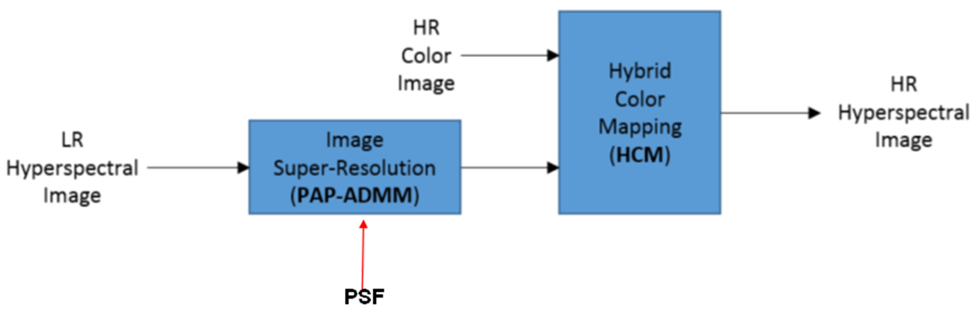
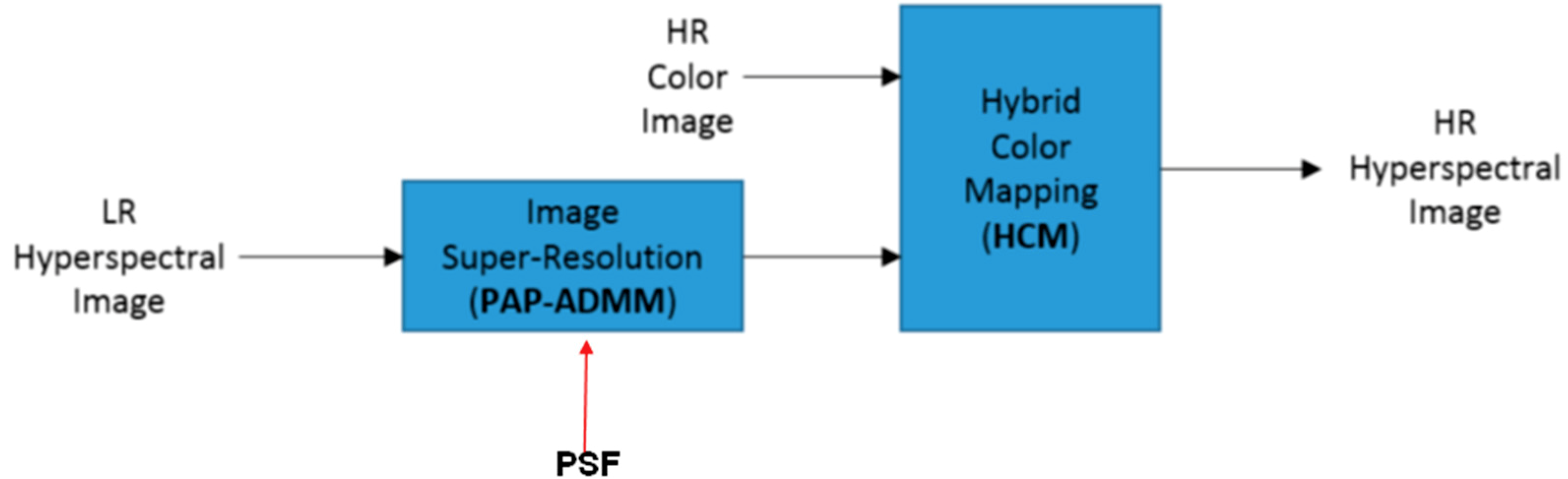
Our proposed algorithm consists of two components as shown in Figure 1. The first component is the incorporation of a single image super-resolution algorithm to enhance the LR HS image cube. Single image super-resolution is a well-studied method in the image processing literature [7,21]. The idea is to up-sample an LR image by using internal image statistics. We chose the PAP-ADMM method [7], which explicitly incorporates PSF into the deblurring and has better performance than other single image super-resolution methods [7]. Our proposed method super-resolves the LR HS images and then fuses the result using the HCM algorithm. The second component utilizes the HCM algorithm [8] that fuses an HR color image with an enhanced HS image coming out of the first component. It should be noted that, since the proposed method is modular in nature, other methods can be used in both steps of the process. For example, we have used other Group 2 methods in Step 2 and found that the results are worse than that of using HCM; reasons can be found in Section 3. Recently, HCM has been applied to several applications, including enhancing Worldview-3 images [30], fusion of Landsat and MODIS images [31], fusion of Worldview and Planet images [32], pansharpening of Mastcam images in the Mars rover Curiosity [33,34], fusing of THEMIS and TES for Mars exploration [35,36], and debayering [37].
Throughout this paper, we use to denote a color image of N pixels, and to denote a HS image of N pixels and P bands. The i-th row of C (and S) is the i-th pixel of the color (and HS) image, and is denoted by (and ). The j-th column of C (and S) is the j-th band of the color (and HS) image, and is denoted by (and ). To differentiate the HR and LR images, we put subscripts H and L to write and for color images, and and for HS images. The number of pixels in an LR image is N and that of an HR image is M. The zoom factor is defined as K = N/M.
We assume that all images have been registered/aligned. Readers interested in image registration can refer to the literature [38,39].
2.1. Hybrid Color Mapping
Consider an LR color pixel and an LR HS pixel , we define the color mapping as a process to determine a linear transformation such that
of which the solution is given by
where and .
The minimization in (1) is generally well-posed because N >> P. In practice, the LR color image can be downsampled from which is assumed to be given.
Equation (2) can be easily derived as follows. The two variables and are related by
Multiplying on both sides yields,
Since is of full-rank, is invertible. Multiplying on both sides of the above equation yields
which is the least square solution shown in Equation (2).
A limitation of the color mapping in (1) is that the wavelengths of the color bands only overlap partially with the hyperspectral bands. For example, color bands in the AVIRIS dataset cover 0.475 μm, 0.51 μm, and 0.65 μm, whereas HS bands cover 0.4–2.5 μm. The long wavelengths in the HS bands are not covered by the color bands.
The hybrid color mapping mitigates the problem by preserving a subset of the higher bands in the HS image. Specifically, we select a subset of HS bands and define
where is the i-th pixel of the jk-th band of the HS image. Note that we also include the white pixel with a value of 1 to adjust for the bias due to the atmospheric effects. Details for the rationale of adding a subset of the HS bands and white pixels can be found in a previous paper [8]. The hybrid linear transformation is therefore
whose solution has the same form as (5). We deliberately use a different notation because and have different dimensions.
Remark 1.
To avoid numerical instability in some situations, (1) can be formulated with a regularization of weights. That is, we can formulate the optimization in the form
The solution for the above equation can be easily shown to be of the form
where I is an identity matrix with the same dimensions as that of .
Remark 2.
For further improvement of the hybrid color mapping, we can divide the image into overlapping patches where each patch has its own T. This tends to improve the performance of the algorithm significantly. Once the transformation T is obtained, the HR HS imagecan be reconstructed by
whereis the given HR color image. The reconstruction ofusingis more challenging because we need the bandsfrom the HR image, which is not yet available. This leads to our next component of using single-image super-resolution to generate those bands.
Remark 3.
Other formulations of the minimization problem shown in (5) have been investigated. For example, instead of using the L2-norm in the regularization term, we have investigated the use of L1-norm and L0-norm. These results have been summarized and published in another paper [40].
2.2. Plug-and-Play ADMM
Plug-and-Play Alternating Direction Method of Multipliers (PAP-ADMM) is a generic optimization algorithm for image restoration problems [7,41]. For the purpose of this paper, we describe PAP-ADMM for recovering HR images from the LR observations. It is emphasized that the PSF is explicitly used in PAP-ADMM to enhance the super-resolution performance.
Consider the j-th band of the hyperspectral image . We denote the HR version of and the LR version of . These two resolutions are related by
where is a convolution matrix representing the blur (i.e., the point spread function (PSF)), is a down-sampling matrix, and is an independent and identically distributed (i.i.d.) Gaussian noise vector. The problem of image super-resolution is to solve an optimization
for some regularization function and parameter , which trades off between the error term and the regularization function in (12).
The PAP-ADMM algorithm is a variant of the classical ADMM algorithm [42] which replaces the regularization function by an implicit regularization function in terms of an image denoiser F. Without going into the details of the PAP-ADMM algorithm (which can be found in a previous study), we summarize the steps involved as follows.
First, we note that (12) is separable and so we can solve each individually. For the j-th band, the algorithm updates iteratively the following quantities.
where and are intermediate variables defined by the PAPADMM algorithm, and is an image denoiser which denoises the input argument with a noise level . In this paper, the image denoiser we use is the Block-Matching and 3D (BM3D) filtering [43], although other denoisers can also be used. The internal parameter is a design parameter and chosen to be 1 based on simulation results.
2.3. Performance Metrics
We evaluate the performance of image reconstruction algorithms using the following objective metrics. Moreover, computational times in seconds are also used in our comparative studies.
• RMSE (Root Mean Squared Error). The RMSE of two HR HS images and is defined as
The ideal value of RMSE is 0 if the image reconstruction is perfect. Since RMSE is a scalar, it does not reveal the RMSE values at different bands. Therefore, we also used , which is the RMSE value between and for each band , to evaluate the performance of different algorithms across individual bands.
- CC (Cross-Correlation). The cross-correlation between and is defined aswith and being the mean of the vector and . The ideal value of CC is 1 if perfect reconstruction is accomplished. We also used , which is the CC value between and for each band, to evaluate the performance of different algorithms across individual bands.
- SAM (Spectral Angle Mapper). The spectral angle mapper is
The ideal value of SAM is 0 for perfect reconstruction. Note that M is the total number of pixels in the image.
• ERGAS (Erreur Relative Globale Adimensionnelle de Synthese). The ERGAS is defined as
for a constant d, which is the ratio of the HR to LR spatial resolutions. The ideal value of ERGAS is 0 if a pansharpening algorithm flawlessly reconstructs the hyperspectral bands.
3. Results
3.1. Data
In this section, we present experimental results along with the conclusions for questions Q1–Q3. We use two hyperspectral image datasets: (1) AF data from the Air Force [44] and (2) AVIRIS data from NASA [45]. The AF image has a size of 267 × 342 × 124, ranging from 0.461 μm to 0.901 μm, meaning that the AF images cover up to the visible and near infrared ranges. The AVIRIS image has a size of 300 × 300 × 213, ranging from 0.38 μm to 2.5 μm. The AVIRIS images cover up to the short-wave infrared (SWIR) range.
To simulate the low-resolution hyperspectral images, we follow the method of a previous paper [4] by downsampling the images spatially with a factor of K = 9 (3 × 3) using a 5 × 5 Gaussian point spread function. The color image RGB channels are taken from the appropriate bands of the HR HS images.
Figure 2 shows a sample band of both datasets.
3.2. Comparison between HCM and PAP-ADMM
Figure 3 illustrates the detailed signal flow of our method. First, given an LR HS image cube, we use PAP-ADMM to generate super-resolution (SR) HS images. Although other single image super-resolution could be used here, we chose PAP-ADMM because it explicitly incorporates PSF and has better performance [7] than other state-of-the-art single resolution methods in the literature. Detailed studies can be found in a previous paper [7]. Second, a subsampling of the SR image and the HR color image is performed. The subsampling is needed in order to allow the compatibility of dimensions between the LR HS image and the LR color image. Third, a mapping T is learned by using the LR color image and the improved LR HS image. This mapping is obtained by minimizing mean square error and an analytical solution can be found. Fourth, an HR hyperspectral image is obtained by multiplying the T matrix with an HR color image. The mapping is done pixel by pixel. Finally, lower bands from the HR hyperspectral image are merged with higher bands in the SR hyperspectral generated by the PAP-ADMM. The reason for this fusion is based on our observation that the higher bands (>0.73 μm for the AF data and >1.88 μm for the AVIRIS data) in the SR image generated by PAP-ADMM have slightly better performance than that of the HCM and the lower bands from HCM that have better performance than those corresponding bands generated by PAP-ADMM. As a result of the fusion, all the bands in the final fused HR HS image are of high quality. For ease of understanding, we also include Algorithm 1 below:
| Algorithm 1 |
| Input: LR HS data, PSF for the hyperspectral imager, and HR color image |
| Output: HR HS data cube |
| Procedures: |
|
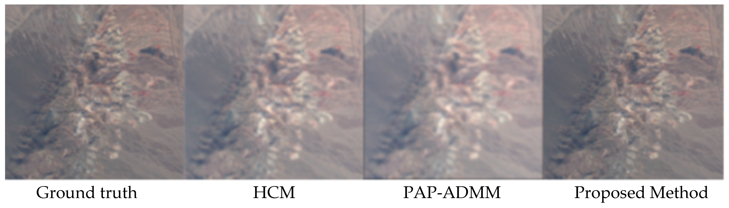
We include an experiment aiming to address the question of why we need both HCM and Plug-and-Play ADMM. The result is shown in Table 1 and Figure 4, where we observe that the integrated approach “PAP-ADMM + HCM” achieves the best performance overall. More results can be found in Table 2 and Figure 5 and Figure 6. The fused approach yielded better values in RMSE, CC, and ERGAS. In terms of subjective performance, one can see from Figure 4 that the fused algorithm achieved high spectral (almost no color distortion) and spatial performance. Such a result is not surprising because PAP-ADMM alone does not utilize the rich information in the color band, whereas the HCM method without an appropriate HR input does not generate a good transformation T. This answers Q1 and Q2.
We should also point out an interesting observation if we look at the RMSE of individual bands. As shown in the plots of Figure 5, the proposed algorithm actually performs well for lower bands (the visible and the near infrared bands). However, for higher bands such as the short wave infrared, PAP-ADMM alone produces the best result (Figure 5). A reason for this is that the color band has diminishing correlation to the higher spectral bands.
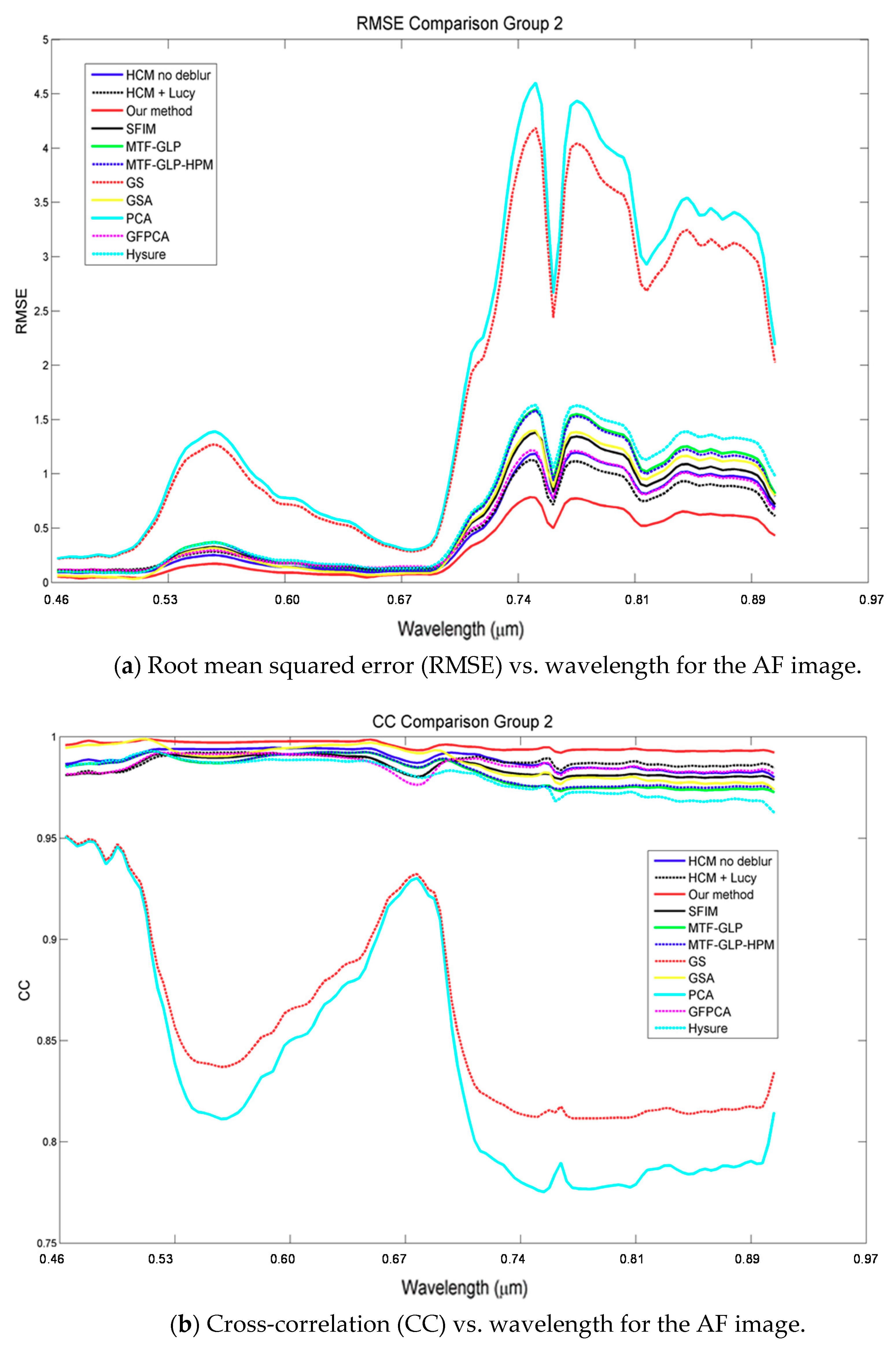
3.3. Comparison with Group 2 Methods
We now compare the proposed algorithm with Group 2 methods. In addition to the proposed algorithm, we also include the basic HCM without deblurring and the HCM results with a conventional deblurring method (Richardson–Lucy [46]). Since our proposed method assumes knowledge about the point spread function (PSF) and a specific image super-resolution algorithm, for fair comparison, we downsample the PAP-ADMM results to simulate a deblurred but downsampled hyperspectral image. Then, we feed the results to Group 2 methods to see if Group 2 methods are improved. The result of this experiment is shown in Table 2. As we can see, this step is detrimental to the performance of Group 2. One reason is that Group 2 methods are already injecting high frequency contents into the hyperspectral images through the pan band. This can be seen from the general formulation of Group 2 methods:
where is the bicubic interpolation, is a gain factor, is the HR pan image, and is a low passed HR pan image. The pan band in this experiment is the average of the 3 color bands from the input image for both the AF and AVIRIS datasets. The reason why Group 2 methods do not benefit from PAP-ADMM is that the residue is the high frequency content injected by the pan band. An additional deblurring step on these Group 2 results tends to overcompensate the effects of the high frequency injection. Therefore, having a strong super-resolution step for Group 2 does not help, and this answers Q3. For completeness, we also include pansharpening results, denoted as 2* in Table 2, of Group 2 methods without deblurring the LR HS images. From those metrics in Table 2, it can be seen that the metrics are indeed better for Group 2 methods if no deblurring is implemented.
In contrast to Group 2 methods, the proposed HCM method benefits significantly from the PAP-ADMM step. One reason is that HCM is using T to generate the HR image and no explicit high frequency contents have been injected yet. This finding also validates the importance of both HCM and PAP-ADMM.
In this experiment, we performed deblurring before we applied the Group 2 methods. As shown in Figure 3, the subsampled image is a deblurred version of the original LR HS image, which we then feed to the Group 2 methods. This will ensure a fair comparison of our method with other Group 2 methods, as all methods will include the preprocessing step of using PAP-ADMM.
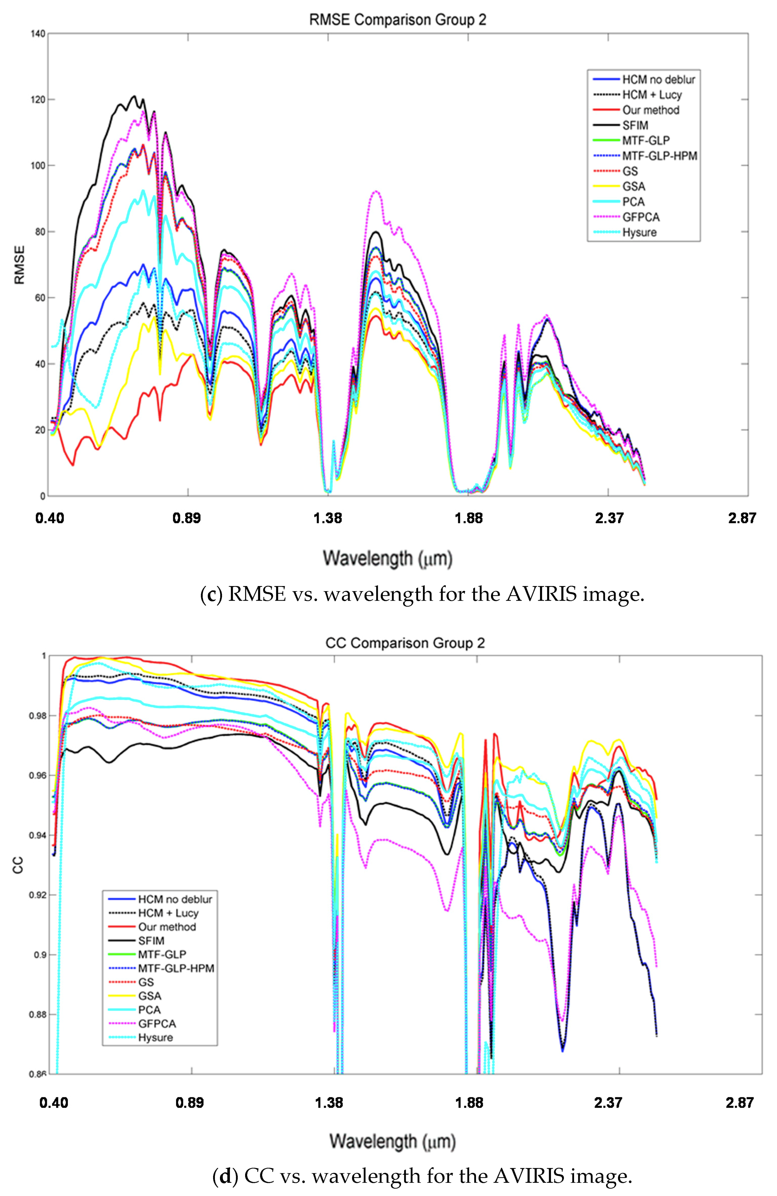
From Figure 5, it can be seen that our method performed consistently well across all bands as compared to other methods in Group 2 for the AF data. In fact, our method yielded the best performance for the AF image in both RMSE and CC as shown in Figure 5a,b and very close to the best performers for the AVIRIS image as shown in Figure 5c,d. Also from Figure 5c,d, it can be seen that our method performed much better in the low bands (<100 or <0.68 μm) as compared to the best performers for the AVIRIS data.
We also notice that Group 2 is inferior to Group 2* because of overcompensation of Group 2 methods due to the deblurring step.
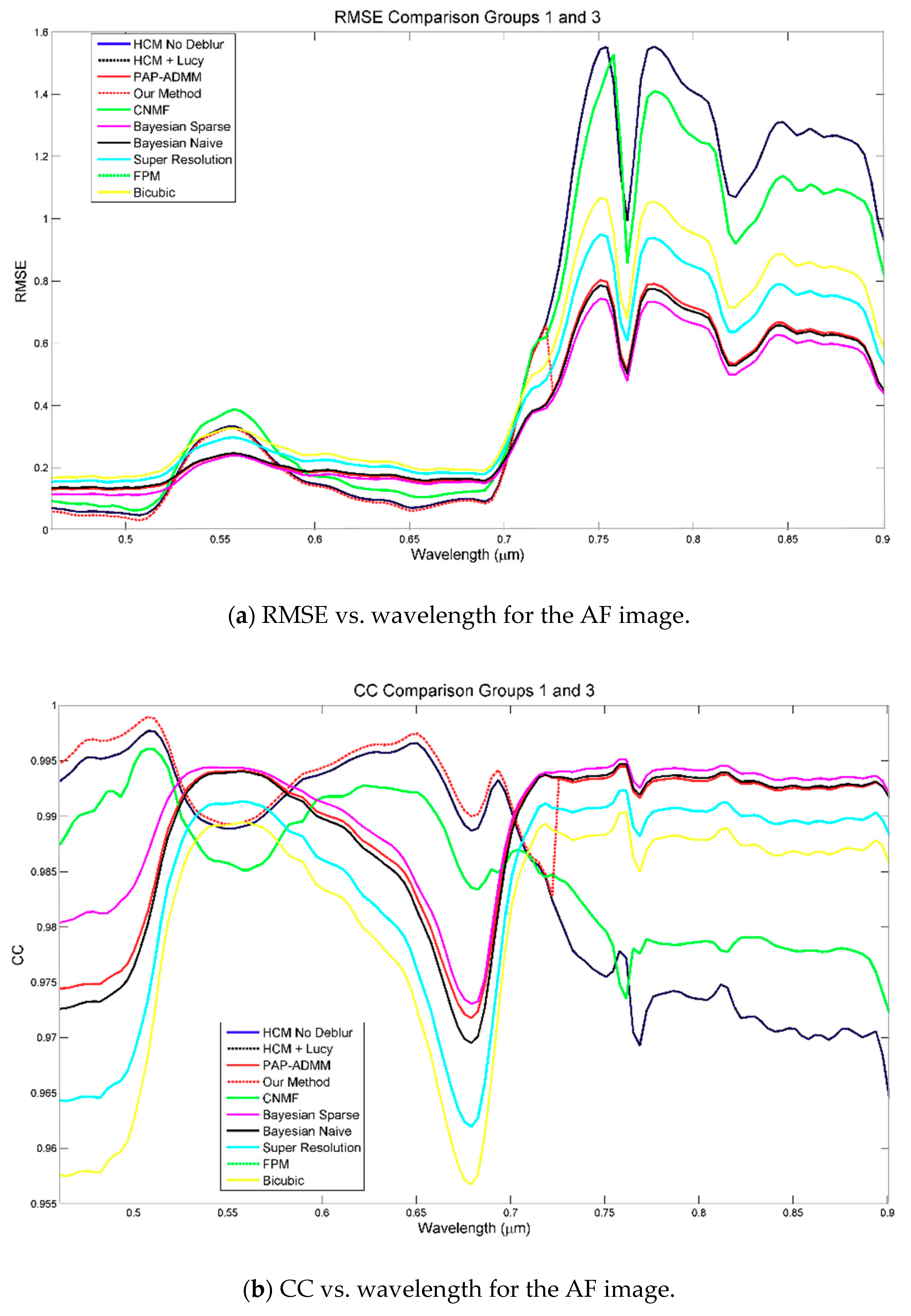
3.4. Comparison with Group 1 and Group 3
We then compare the performance of the proposed algorithm with Group 1 and Group 3 methods. Table 2 shows the performance metrics. The average RMSE of our method is very close to that of Bayesian Sparse for the AF data and much better for the AVIRIS data. However, if we inspect Figure 6a,c closely, we see that our method actually has a lower RMSE for a majority of the low bands. Moreover, if we look at the AVIRIS’s RMSE in Figure 6c, we observe that even at higher bands our performance is comparable to those Group 1 methods. The performance in AF’s CC plot shown in Figure 6b is even more dramatic, as our results in red achieved near or above 0.995 for all bands. Therefore, if multispectral images with some bands in the high bands could be used, our proposed method can possibly achieve even better results.
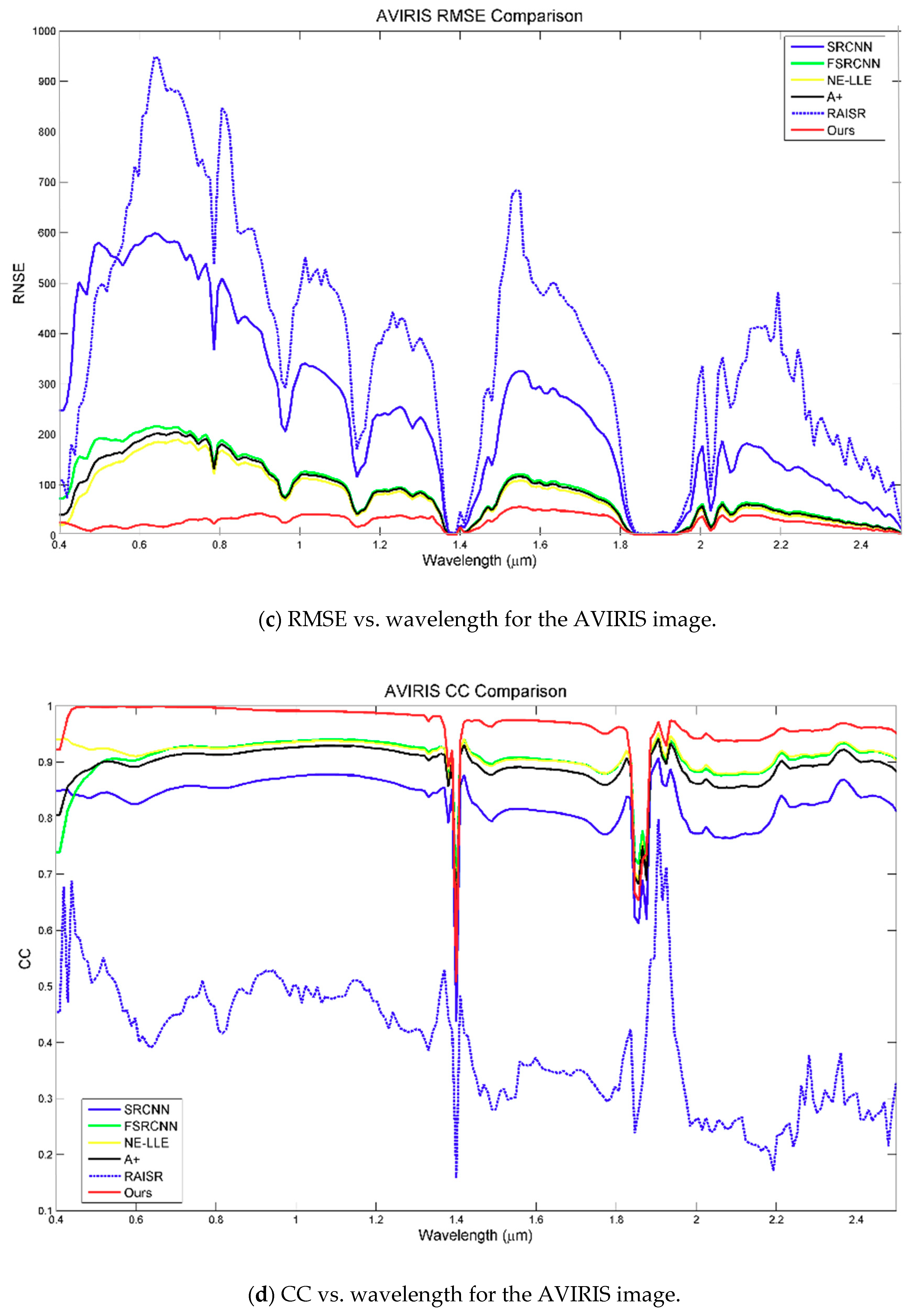
3.5. Comparison with Group 4
As mentioned earlier, Group 4 methods also are single image super-resolution methods, except that they utilize some additional dictionaries and training images. In particular, the methods in the literature [24,25] use training images to build dictionaries and the methods in other past papers [26,27] use many training images and deep learning algorithms to train models. Table 2 and Figure 7 summarize the comparison between our approach and those Group 4 methods. It can be seen that our approach outperformed all the Group 4 methods. There are several explanations. First, Group 4 methods do not incorporate PSF information. Second, all these Group 4 methods require a lot of training images that are relevant to the dataset being tested, which we do not have. The training images commonly used for these methods, specifically SRCNN and FSRCNN, do not necessarily provide relevant information to improving the quality of hyperspectral images. We should also mention that the deep learning based methods are extremely time consuming (applicable datasets can take hundreds of hours on an average PC) in training, which may prohibit practical applications.
3.6. Visualization of Fused Images Using Different Methods
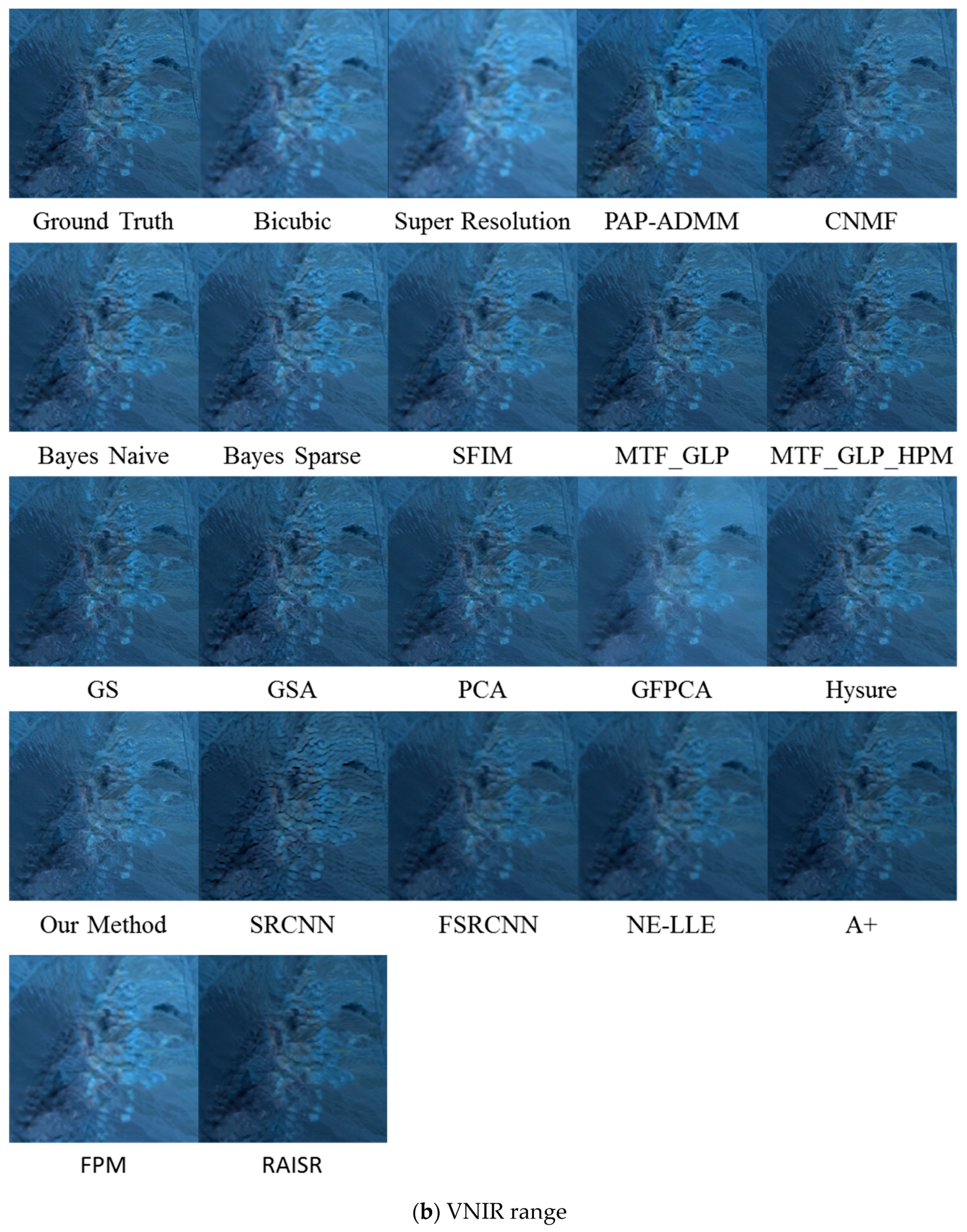
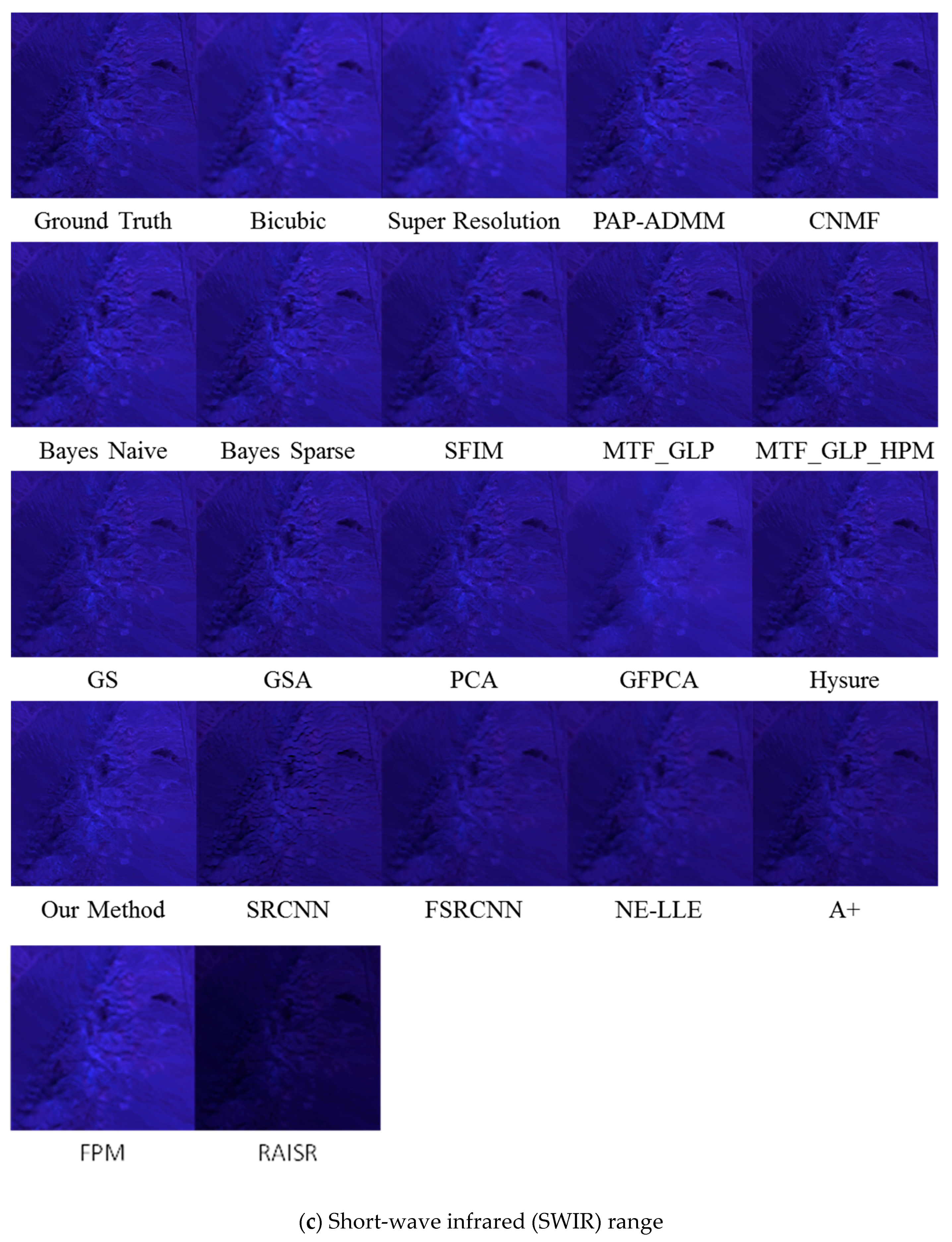
Here, we present a subjective comparison of fused images using our method and all methods mentioned in Groups 1 to 4. Figure 8 shows the synthesized color images from the fused AF hyperspectral image in visible range using bands (0.47 μm, 0.51 μm, and 0.65 μm) and VNIR (visible near infrared) range using bands (0.70 μm, 0.77 μm, and 0.85 μm), respectively. In order to compare the performance of different methods, we selected only ten images for display in Figure 8. Other images can be requested by contacting us. Our method can be seen to preserve the spectral fidelity quite well. For example, one can look at the color of the grass and tree areas between our fused image and the reference image. There is almost no color distortion between our results and the reference image. In contrast, some methods such as CNMF, GSA, RAISR, etc. clearly have strong spectral/color distortions in the VNIR range. For completeness, we also include the synthesized color images in three spectral ranges of the fused AVIRIS image in Figure 9. Similar to the AF images, we selected ten images for display and the rest can be requested by contacting us. However, it is somewhat hard to see the subtle differences between different methods. Nevertheless, results from some methods such as GFPCA and single image super-resolution obviously have large spectral distortions. For AVIRIS data, the visible, VNIR (visible near infrared) and SWIR (short wave infrared) images were formed by using bands (0.47 μm, 0.57 μm, and 0.66 μm), (0.89 μm, 1.08 μm, and 1.28 μm), and (1.58 μm, 1.98 μm, and 2.37 μm), respectively.
3.7. Performance Comparison of Different Algorithms Using Pixel Clustering
In addition to the objective and subjective evaluations discussed in Section 3.3, Section 3.4, Section 3.5 and Section 3.6, pixel clustering was performed to further validate our previous results. Pixel clustering was not performed in any of the competitive approaches [9,10,11,12,13,14,15,16,17,18,19,20,21,22,23,24,25,26,27].
We would like to emphasize the following points:
- This study is for pixel clustering, not for land cover classification. In land cover classification, it is normally required to have reflectance signatures of different land covers and the raw radiance images need to be atmospherically compensated to eliminate atmospheric effects.
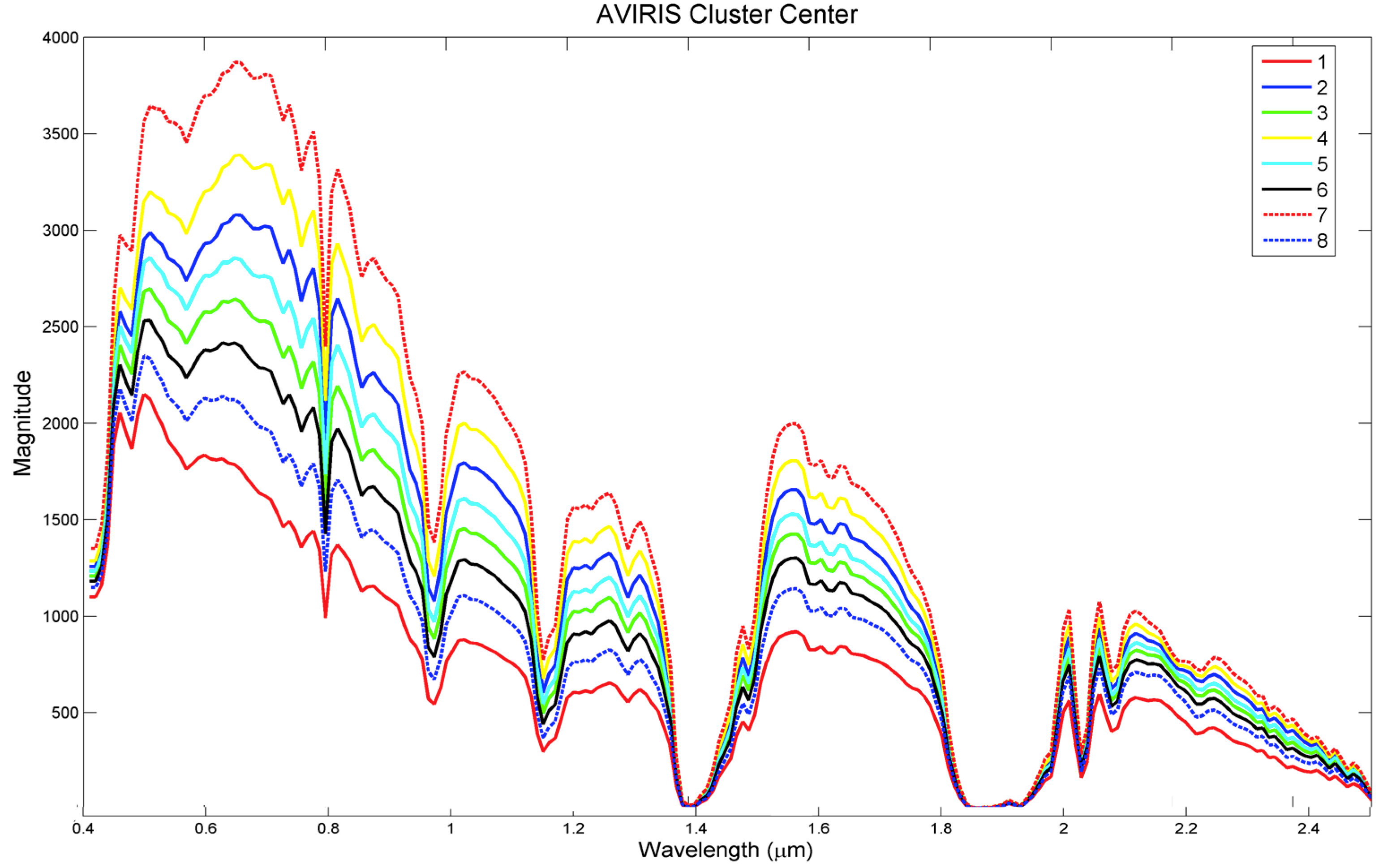
- Because our goal is for pixel clustering, we worked directly in the radiance domain without any atmospheric compensation. We carried out the clustering using k-means algorithm. The number of clusters selected was eight in both the AF and the AVIRIS data sets. Although other numbers could be chosen, we felt that eight clusters would adequately represent the variation of pixels in these images. The eight signatures or cluster means of AF and AVIRIS data sets are shown in Figure 10 and Figure 11, respectively. It can be seen that the clusters are quite distinct.
- Moreover, since our focus is on pixel clustering performance of different pansharpening algorithms, the physical meaning or type of material in each cluster is not the concern of our study.
- A pixel is considered to belong to a particular cluster if its distance to that cluster center is the shortest. Here, distance is defined as the Euclidean distance between two pixel vectors. The main reason is that some of the cluster means in Figure 10 and Figure 11 have similar spectral shapes. If we use spectral angle difference, then there will be many incorrect results.
- It is our belief that if a pansharpening algorithm can preserve the spatial and spectral integrity in terms of RMSE, CC, ERGAS, SAM, and can also achieve a high clustering accuracy, it should be regarded as a high performing algorithm.
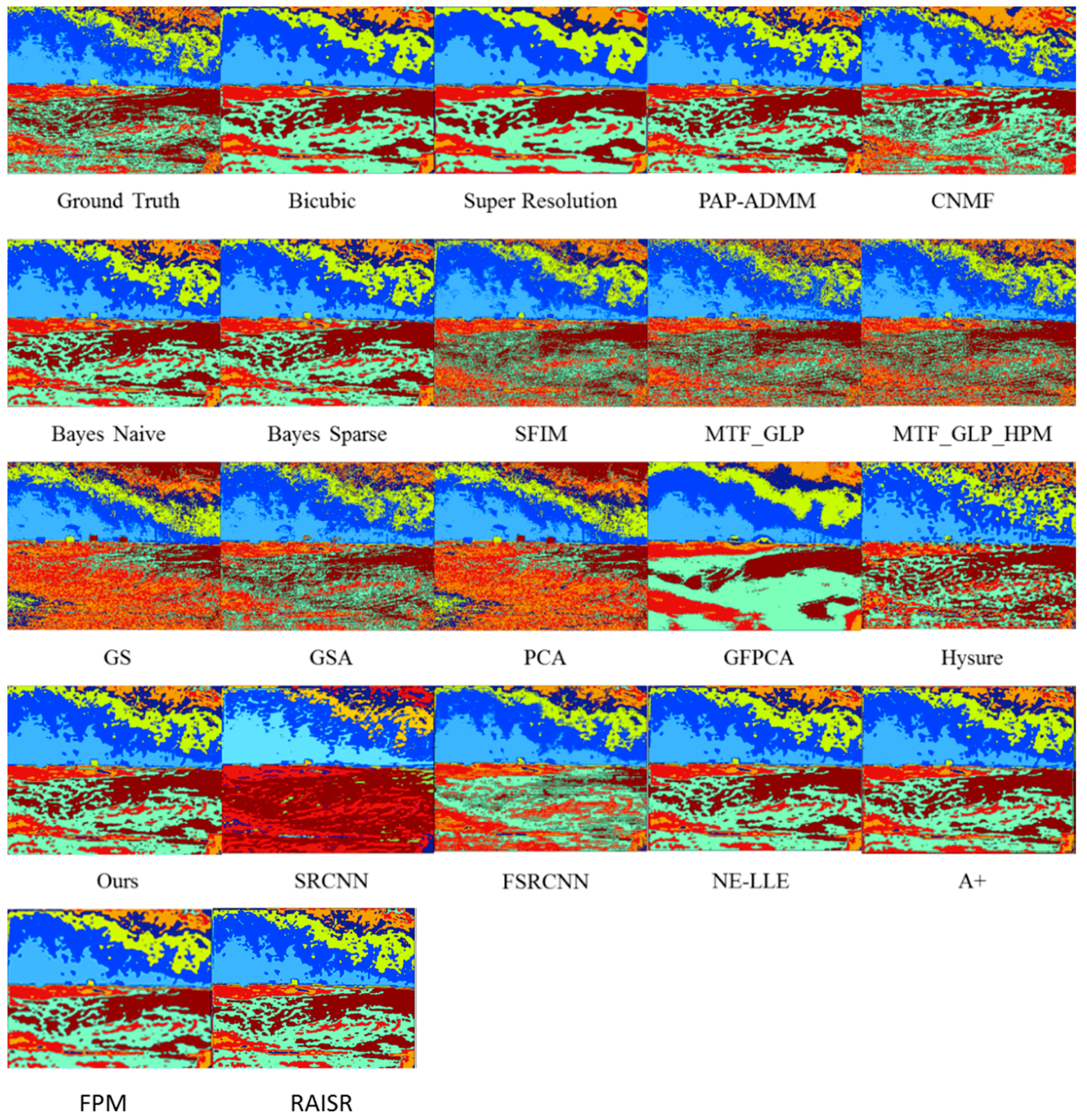
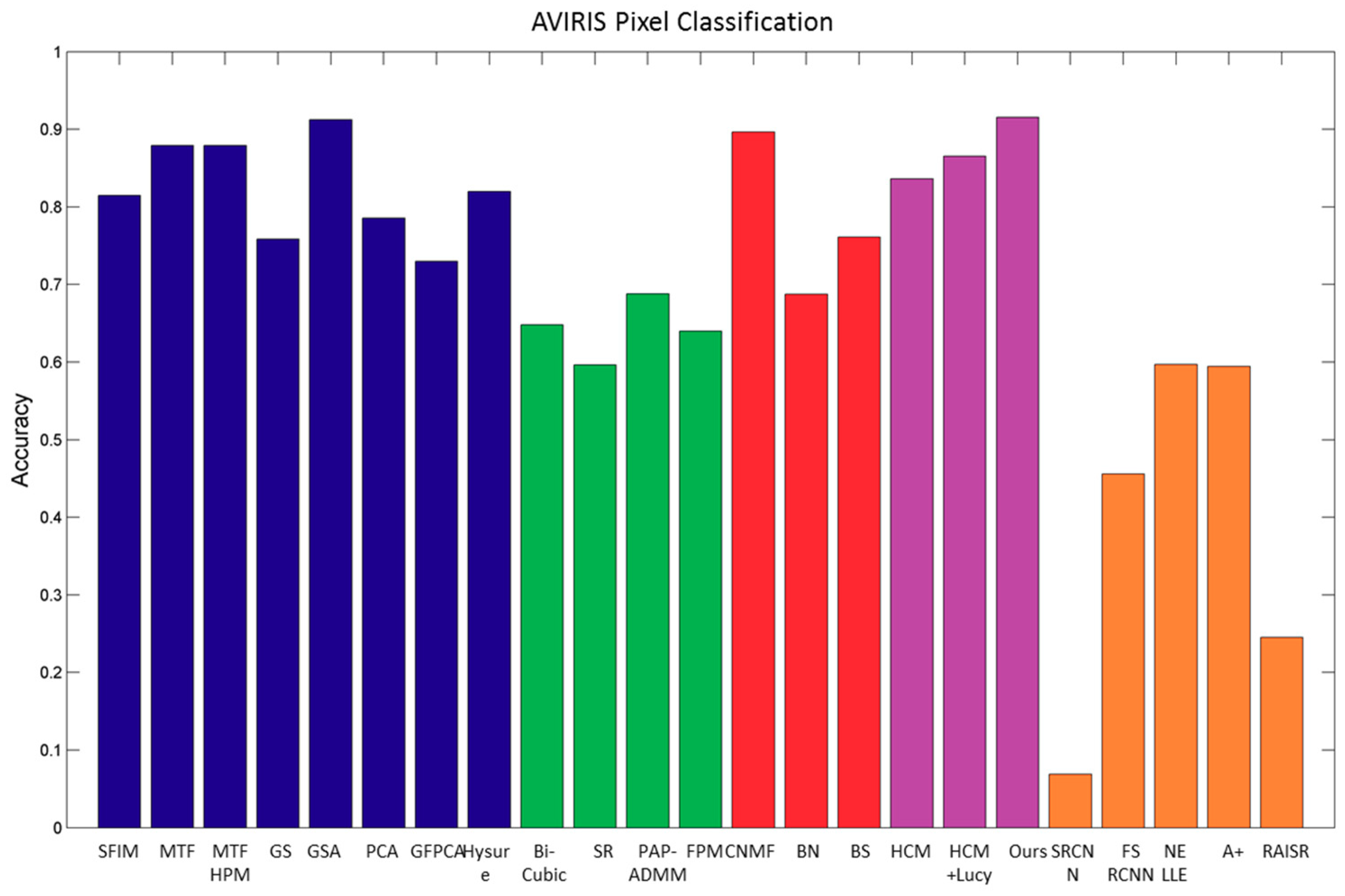
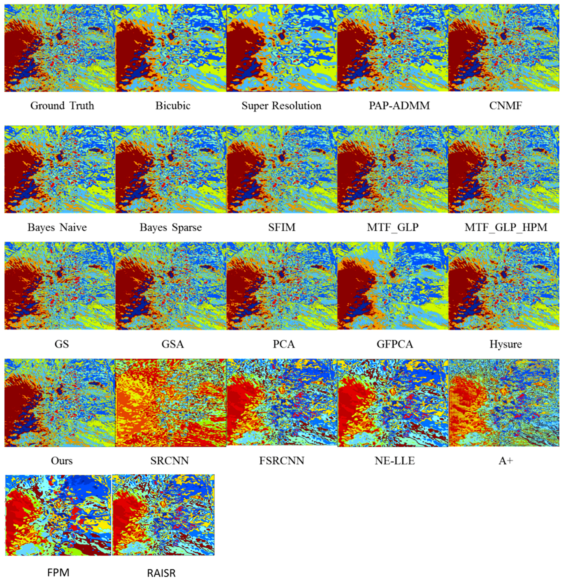
Figure 12, Figure 13, Figure 14 and Figure 15 show the clustering results from different pansharpening methods based on cluster centers extracted from ground truth AF and AVIRIS hyperspectral images, respectively. We used K-means endmember extraction technique to determine the cluster centers. It can be seen that our method, together with several others, produced the best clustering performance as shown in Figure 12, Figure 13, Figure 14 and Figure 15. Compared with the best method in Group 1 for the AVIRIS data, which is PAP-ADMM, our method was 20% more accurate to the ground truth. The best Group 2 method is GFPCA for the AF data and MTF-GLP for the AVIRIS. Our method is better than GFPCA for the AF data and is comparable to MTF-GLP for the AVIRIS data. Comparing with the methods of Groups 3 and 4, our proposed method yielded better performance. From a previous study [4], it was observed that the Bayesian sparse (BS) algorithm performed consistently well for all the data sets in [4]. However, this is not the case for the AVIRIS data because CNMF has better performance than those Bayesian methods. Moreover, our method yielded more than 2 to 3% better performance than that of the best Group 1 method (CNMF) for the AVIRIS data. This means that the performance of pansharpening is data dependent and it is worth experimenting with different algorithms for a new application. The cluster maps of all the algorithms are shown in Figure 13 and Figure 15. It can be seen from Figure 13 that cluster maps from the top performers (BS, our proposed method, and PAP-ADMM) are more comparable to the reference map (ground truth). GS, PCA, and SRCNN had a lot of misclassifications. GFPCA tends to lump small clusters into big clusters. Others seem to have comparable performance. Looking at Figure 15, we can observe that the methods of Groups 3 and 4 do not perform well. The high performing ones are CNMF, GSA, and our method. We also notice that in both Figure 13 and Figure 15, the bicubic, SR, and GFPCA do not yield fine clusters, as compared to others. Finally, the clustering performance of different methods in the two images can vary quite a lot. For example, CNMF performed well for AVIRIS image but not the AF image; BS worked well for the AF image, but not the AVIRIS image. This indicates the necessity of having different algorithms to meet different applications. The consistent ones in both images are the proposed method and some of the Group 2 methods (GSA, MTF, and MTF-HPM).
4. Discussion
Fusion of an HR color image with an LR HS image can yield an HR HS image. Although there are quite a few algorithms in the literature in recent years to address problems similar to the above, there is still room for further improvement. Our paper presents a new fusion algorithm that can generate HR HS images with help from HR color images. We have thoroughly compared our algorithm with more than 15 algorithms, divided into four groups, in the literature.
It should be noted that the methods of Group 1 have explicitly incorporated PSF into their algorithms, but not for directly deblurring of the hyperspectral bands. Our approach is to explicitly use PSF to perform deblurring.
We would like to mention that HCM and PAP-ADMM are complementary to each other. HCM can achieve high performance in the low number bands, as there is more correlation between the color bands and those low number bands. In fact, we have two ways to incorporate additional information from the higher spectral bands to improve the HCM. One is to include some hyperspectral bands in our mapping; see Equation (3) in our paper. Another way is to utilize deblurred results by using PAP-ADMM.
It is also interesting to see that the methods of Group 2 cannot benefit from the proposed approach. This is because the methods of Group 2 have an inherent mechanism to inject high frequency spectral information to enhance the LR HS images. Additional deblurring overcompensates for the enhancement process and is hence detrimental to the image quality. In contrast, HCM can benefit from deblurring from PAP-ADMM.
In terms of objective evaluations, we have used five performance metrics, which are widely used in the literature, to compare the results of each algorithm. It was observed that our algorithm performed better than the methods of Group 3 from Table 2 and Figure 6. Our method also performed better than most of the Group 1 methods for the AF image (Figure 5) and is comparable to the best Group 2 methods for the AVIRIS image (Figure 5). Comparing with Group 1 methods, our algorithm yielded a consistently high performance for all bands (Figure 6). For example, for the results related to AF image in Figure 6a, our performance is much better than CNMF in almost all bands. Comparing with Group 4 methods, our algorithm performed better in all cases (Figure 7).
In terms of subjective visualization, one can see that our results are comparable or better than others. In particular, if one looks at the VNIR bands in the AF image (Figure 8b), it can be clearly seen that our results preserve the spectral integrity better than almost all the others. Some well-known methods such as GS, GSA, and CNMF have large spectral distortions in the VNIR bands.
5. Conclusions
A new fusion based algorithm to enhance the resolution of hyperspectral images is presented. In addition to the LR HS image, an HR color image is needed. Our new algorithm is an integration of a hybrid color mapping algorithm and a single image super-resolution algorithm. Although the new approach is simple, the performance is promising based on a comparative study with 20 existing algorithms using five objective metrics, subjective visualization in multiple spectral ranges (visible, VNIR, SWIR), and pixel clustering accuracy on real image datasets.
Author Contributions
C.K. conceived the overall approach and wrote the paper. J.H.C. and S.C. provided inputs related to the PAP-ADMM algorithm and also the deblurring results. J.Z. provided inputs related to HCM. B.B. generated all the figures and tables.
Funding
This research received no external funding.
Conflicts of Interest
The authors declare no conflict of interest.
References
- Lee, C.M.; Cable, M.L.; Hook, S.J.; Green, R.O.; Ustin, S.L.; Mandl, D.J.; Middleton, E.M. An introduction to the NASA hyperspectral infrared imager (hyspiri) mission and preparatory activities. Remote Sens. Environ. 2015, 167, 6–19. [Google Scholar] [CrossRef]
- Kwan, C.; Yin, J.; Zhou, J.; Chen, H.; Ayhan, B. Fast Parallel Processing Tools for Future HyspIRI Data Processing. In Proceedings of the NASA HyspIRI Science Symposium, Greenbelt, MD, USA, 29–30 May 2013. [Google Scholar]
- Zhou, J.; Chen, H.; Ayhan, B.; Kwan, C. A High Performance Algorithm to Improve the Spatial Resolution of HyspIRI Images. In Proceedings of the NASA HyspIRI Science and Applications Workshop, Washington, DC, USA, 16 October 2012. [Google Scholar]
- Loncan, L.; de Almeida, L.B.; Bioucas-Dias, J.M.; Briottet, X.; Chanussot, J.; Dobigeon, N.; Fabre, S.; Liao, W.; Licciardi, G.A.; Simoes, M.; et al. Hyperspectral pansharpening: A review. IEEE Geosci. Remote Sens. Mag. 2015, 3, 27–46. [Google Scholar] [CrossRef]
- Schowengerdt, R.A. Remote Sensing: Models and Methods for Image Processing; Academic Press: Cambridge, MA, USA, 1997. [Google Scholar]
- Kwan, C.; Dao, M.; Chou, B.; Kwan, L.M.; Ayhan, B. Mastcam Image Enhancement Using Estimated Point Spread Functions. In Proceedings of the IEEE Ubiquitous Computing, Electronics & Mobile Communication Conference, New York, NY, USA, 19–21 October 2017. [Google Scholar]
- Chan, S.H.; Wang, X.; Elgendy, O.A. Plug-and-play admm for image restoration: Fixed point convergence and applications. IEEE Trans. Comput. Imaging 2017, 3, 84–98. [Google Scholar] [CrossRef]
- Zhou, J.; Kwan, C.; Budavari, B. Hyperspectral image super-resolution: A hybrid color mapping approach. J. Appl. Remote Sens. 2016, 10, 035024. [Google Scholar] [CrossRef]
- Yokoya, N.; Yairi, T.; Iwasaki, A. Coupled nonnegative matrix factorization unmixing for hyperspectral and multispectral data fusion. IEEE Trans. Geosci. Remote Sens. 2012, 50, 528–537. [Google Scholar] [CrossRef]
- Hardie, R.C.; Eismann, M.T.; Wilson, G.L. Map estimation for hyperspectral image resolution enhancement using an auxiliary sensor. IEEE Trans. Image Process. 2004, 13, 1174–1184. [Google Scholar] [CrossRef] [PubMed]
- Wei, Q.; Bioucas-Dias, J.; Dobigeon, N.; Tourneret, J.Y. Hyperspectral and multispectral image fusion based on a sparse representation. IEEE Trans. Geosci. Remote Sens. 2015, 53, 3658–3668. [Google Scholar] [CrossRef]
- Chavez, P.S., Jr.; Sides, S.C.; Anderson, J.A. Comparison of three different methods to merge multiresolution and multispectral data: Landsat tm and spot panchromatic. Photogramm. Eng. Remote Sens. 1991, 57, 295–303. [Google Scholar]
- Liao, W.; Huang, X.; Coillie, F.V.; Gautama, S.; Pizurica, A.; Philips, W.; Liu, H.; Zhu, T.; Shimoni, M.; Moser, G.; et al. Processing of multiresolution thermal hyperspectral and digital color data: Outcome of the 2014 IEEE grss data fusion contest. IEEE J. Sel. Top. Appl. Earth Obs. Remote Sens. 2015, 8, 2984–2996. [Google Scholar] [CrossRef]
- Laben, C.; Brower, B. Process for Enhancing the Spatial Resolution of Multispectral Imagery Using Pan-Sharpening. U.S. Patent 6,011,875, 4 January 2000. [Google Scholar]
- Aiazzi, B.; Baronti, S.; Selva, M. Improving component substitution pansharpening through multivariate regression of ms+pan data. IEEE Trans. Geosci. Remote Sens. 2007, 45, 3230–3239. [Google Scholar] [CrossRef]
- Aiazzi, B.; Alparone, L.; Baronti, S.; Garzelli, A.; Selva, M. MTF-tailored multiscale fusion of high-resolution ms and pan imagery. Photogramm. Eng. Remote Sens. 2006, 72, 591–596. [Google Scholar] [CrossRef]
- Vivone, G.; Restaino, R.; Dalla Mura, M.; Licciardi, G.; Chanussot, J. Contrast and error-based fusion schemes for multispectral image pansharpening. IEEE Geosci. Remote Sens. Lett. 2014, 11, 930–934. [Google Scholar] [CrossRef]
- Simoes, M.; Bioucas-Dias, J.; Almeida, L.B.; Chanussot, J. A convex formulation for hyperspectral image superresolution via subspace-based regularization. IEEE Trans. Geosci. Remote Sens. 2015, 53, 3373–3388. [Google Scholar] [CrossRef]
- Simoes, M.; Bioucas-Dias, J.; Almeida, L.B.; Chanussot, J. Hyperspectral image superresolution: An edge-preserving convex formulation. In Proceedings of the 2014 IEEE International Conference on Image Processing (ICIP), Paris, France, 27–30 October 2014; pp. 4166–4170. [Google Scholar]
- Liu, J.G. Smoothing filter based intensity modulation: A spectral preserve image fusion technique for improving spatial details. Int. J. Remote Sens. 2000, 21, 3461–3472. [Google Scholar] [CrossRef]
- Yan, Q.; Xu, Y.; Yang, X.; Truong, T.Q. Single image superresolution based on gradient profile sharpness. IEEE Trans. Image Process. 2015, 24, 3187–3202. [Google Scholar] [PubMed]
- Keys, R. Cubic convolution interpolation for digital image processing. IEEE Trans. Acoust. Speech Signal Process. 1981, 29, 1153–1160. [Google Scholar] [CrossRef] [Green Version]
- Desai, D.B.; Sen, S.; Zhelyeznyakov, M.V.; Alenazi, W.; de Peralta, L.G. Super-resolution imaging of photonic crystals using the dual-space microscopy technique. Appl. Opt. 2016, 55, 3929–3934. [Google Scholar] [CrossRef] [PubMed]
- Timofte, R.; de Smet, V.; Van Gool, L. A+: Adjusted anchored neighborhood regression for fast super-resolution. In Proceedings of the Asian Conference on Computer Vision, Singapore, 1–5 November 2014; pp. 111–126. [Google Scholar]
- Chang, H.; Yeung, D.; Xiong, Y. Super-resolution through neighbor embedding. In Proceedings of the 2004 IEEE Computer Society Conference on Computer Vision and Pattern Recognition, Washington, DC, USA, 27 June–2 July 2004. [Google Scholar]
- Dong, C.; Loy, C.C.; He, K.; Tang, X. Learning a deep convolutional network for image super-resolution. In Proceedings of the European Conference on Computer Vision, Zurich, Switzerland, 6–12 September 2014; pp. 184–199. [Google Scholar]
- Dong, C.; Loy, C.C.; Tang, X. Accelerating the super-resolution convolutional neural network. In Proceedings of the European Conference on Computer Vision, Amsterdam, The Netherlands, 8–16 October 2016; pp. 391–407. [Google Scholar]
- Romano, Y.; Isidoro, J.; Milanfar, P. RAISR: Rapid and accurate image super resolution. IEEE Trans. Comput. Imaging 2017, 3, 110–125. [Google Scholar] [CrossRef]
- Kwan, C.; Choi, J.H.; Chan, S.; Zhou, J.; Budavari, B. Resolution Enhancement for Hyperspectral Images: A Super-Resolution and Fusion Approach. In Proceedings of the IEEE International Conference on Acoustics, Speech, and Signal Processing, New Orleans, LA, USA, 5–9 March 2017; pp. 6180–6184. [Google Scholar]
- Kwan, C.; Budavari, B.; Bovik, A.C.; Marchisio, G. Blind Quality Assessment of Fused WorldView-3 Images by Using the Combinations of Pansharpening and Hypersharpening Paradigms. IEEE Geosci. Remote Sens. Lett. 2017, 14, 1835–1839. [Google Scholar] [CrossRef]
- Kwan, C.; Budavari, B.; Gao, F.; Zhu, X. A Hybrid Color Mapping Approach to Fusing MODIS and Landsat Images for Forward Prediction. Remote Sens. 2018, 10, 520. [Google Scholar] [CrossRef]
- Kwan, C.; Zhu, X.; Gao, F.; Chou, B.; Perez, D.; Li, J.; Shen, Y.; Koperski, K.; Marchisio, G. Assessment of Spatiotemporal Fusion Algorithms for Worldview and Planet Images. Sensors 2018, 18, 1051. [Google Scholar] [CrossRef] [PubMed]
- Kwan, C.; Budavari, B.; Dao, M.; Ayhan, B.; Bell, J.F. Pansharpening of Mastcam images. In Proceedings of the IEEE International Geoscience and Remote Sensing Symposium (IGARSS), Fort Worth, TX, USA, 23–28 July 2017; pp. 5117–5120. [Google Scholar]
- Dao, M.; Kwan, C.; Ayhan, B.; Bell, J.F. Enhancing Mastcam Images for Mars Rover Mission. In Proceedings of the 14th International Symposium on Neural Networks, Hokkaido, Japan, 21–26 June 2017; pp. 197–206. [Google Scholar]
- Kwan, C.; Ayhan, B.; Budavari, B. Fusion of THEMIS and TES for Accurate Mars Surface Characterization. In Proceedings of the IEEE International Geoscience and Remote Sensing Symposium (IGARSS), Fort Worth, TX, USA, 23–28 July 2017; pp. 3381–3384. [Google Scholar]
- Kwan, C.; Haberle, C.; Ayhan, B.; Chou, B.; Echavarren, A.; Castaneda, G.; Budavari, B.; Dickenshied, S. On the Generation of High-Spatial and High-Spectral Resolution Images Using THEMIS and TES for Mars Exploration. In Proceedings of the SPIE Defense + Security Conference, Orlando, FL, USA, 10–13 April 2018. [Google Scholar]
- Kwan, C.; Chou, B.; Kwan, L.M.; Budavari, B. Debayering RGBW Color Filter Arrays: A Pansharpening Approach. In Proceedings of the IEEE Ubiquitous Computing, Electronics & Mobile Communication Conference, New York, NY, USA, 19–21 October 2017. [Google Scholar]
- Horn, B.K.P.; Schunck, B.G. Determining optical flow. Artif. Intell. 1981, 17, 185–203. [Google Scholar] [CrossRef] [Green Version]
- Barron, J.L.; Fleet, D.J.; Beauchemin, S.S. Performance of optical flow techniques. Int. J. Comput. Vis. 1994, 12, 43–77. [Google Scholar] [CrossRef] [Green Version]
- Kwan, C.; Budavari, B.; Dao, M.; Zhou, J. New Sparsity Based Pansharpening Algorithm for Hyperspectral Images. In Proceedings of the IEEE Ubiquitous Computing, Electronics & Mobile Communication Conference, New York, NY, USA, 19–21 October 2017. [Google Scholar]
- Sreehari, S.; Venkatakrishnan, S.V.; Wohlberg, B.; Drummy, L.F.; Simmons, J.P.; Bouman, C.A. Plug-and-play priors for bright field electron tomography and sparse interpolation. IEEE Trans. Comput. Imaging 2016, 2, 408–423. [Google Scholar] [CrossRef]
- Boyd, S.; Parikh, N.; Chu, E.; Peleato, B.; Eckstein, J. Distributed optimization and statistical learning via the alternating direction method of multipliers. Found. Trends Mach. Learn. 2011, 3, 1–122. [Google Scholar]
- Dabov, K.; Foi, A.; Katkovnik, V.; Egiazarian, K. Image denoising by sparse 3-d transform-domain collaborative filtering. IEEE Trans. Image Process. 2007, 16, 2080–2095. [Google Scholar] [CrossRef] [PubMed]
- Zhou, J.; Kwan, C.; Ayhan, B.; Eismann, M. A Novel Cluster Kernel RX Algorithm for Anomaly and Change Detection Using Hyperspectral Images. IEEE Trans. Geosci. Remote Sens. 2016, 54, 6497–6504. [Google Scholar] [CrossRef]
- Hook, S.J.; Rast, M. Mineralogic mapping using airborne visible infrared imaging spectrometer (aviris), shortwave infrared (swir) data acquired over cuprite, Nevada. In Proceedings of the Second Airborne Visible Infrared Imaging Spectrometer (AVIRIS) Workshop, Pasadena, CA, USA, 4–5 June 1990; pp. 199–207. [Google Scholar]
- Fish, D.A.; Walker, J.G.; Brinicombe, A.M.; Pike, E.R. Blind deconvolution by means of the Richardson-Lucy algorithm. J. Opt. Soc. Am. A 1995, 12, 58–65. [Google Scholar] [CrossRef]
Figure 1.
Outline of the proposed method. We use hybrid color mapping (HCM) to fuse low-resolution (LR) and high-resolution (HR) images. For LR images, we use a single-image super-resolution algorithm where PSF is incorporated to first enhance the resolution before feeding to the HCM.
Figure 1.
Outline of the proposed method. We use hybrid color mapping (HCM) to fuse low-resolution (LR) and high-resolution (HR) images. For LR images, we use a single-image super-resolution algorithm where PSF is incorporated to first enhance the resolution before feeding to the HCM.

Figure 2.
(a) is a sample band from AF data and (b) is a sample band from AVIRIS data.
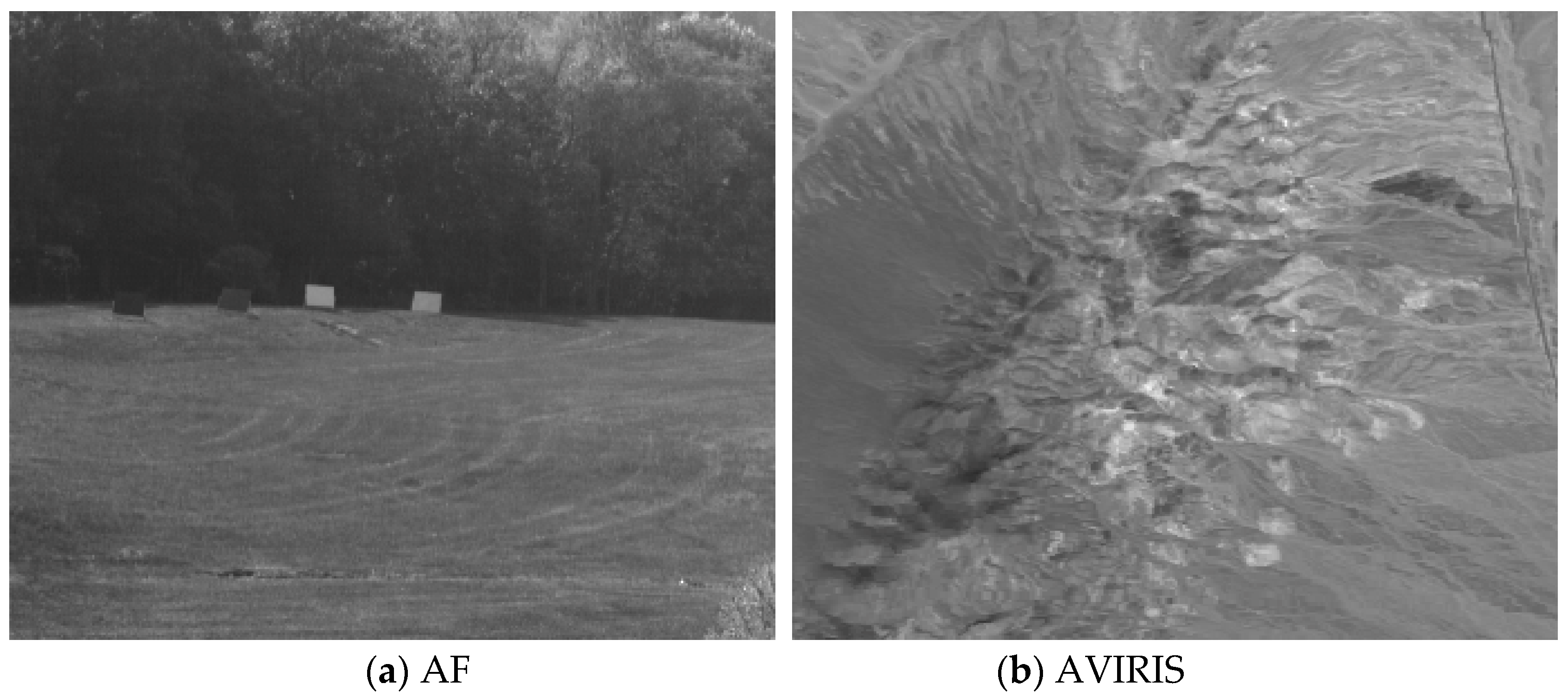
Figure 3.
Signal flow of our method.
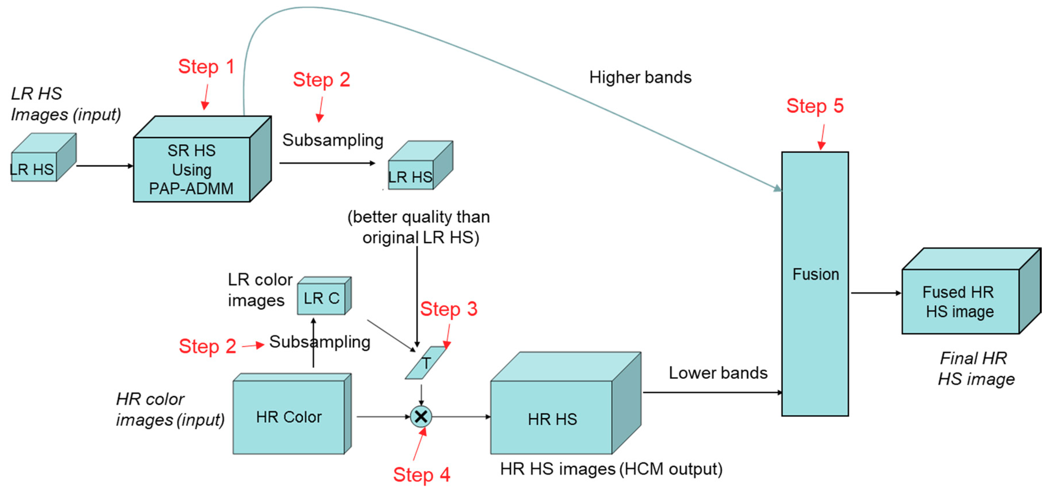
Figure 4.
AVIRIS images in visible range using different methods.

Figure 5.
Comparison of RMSE and CC between our method and methods from Group 2.


Figure 6.
Comparison of RMSE and CC between our method and methods in Groups 1 and 3.

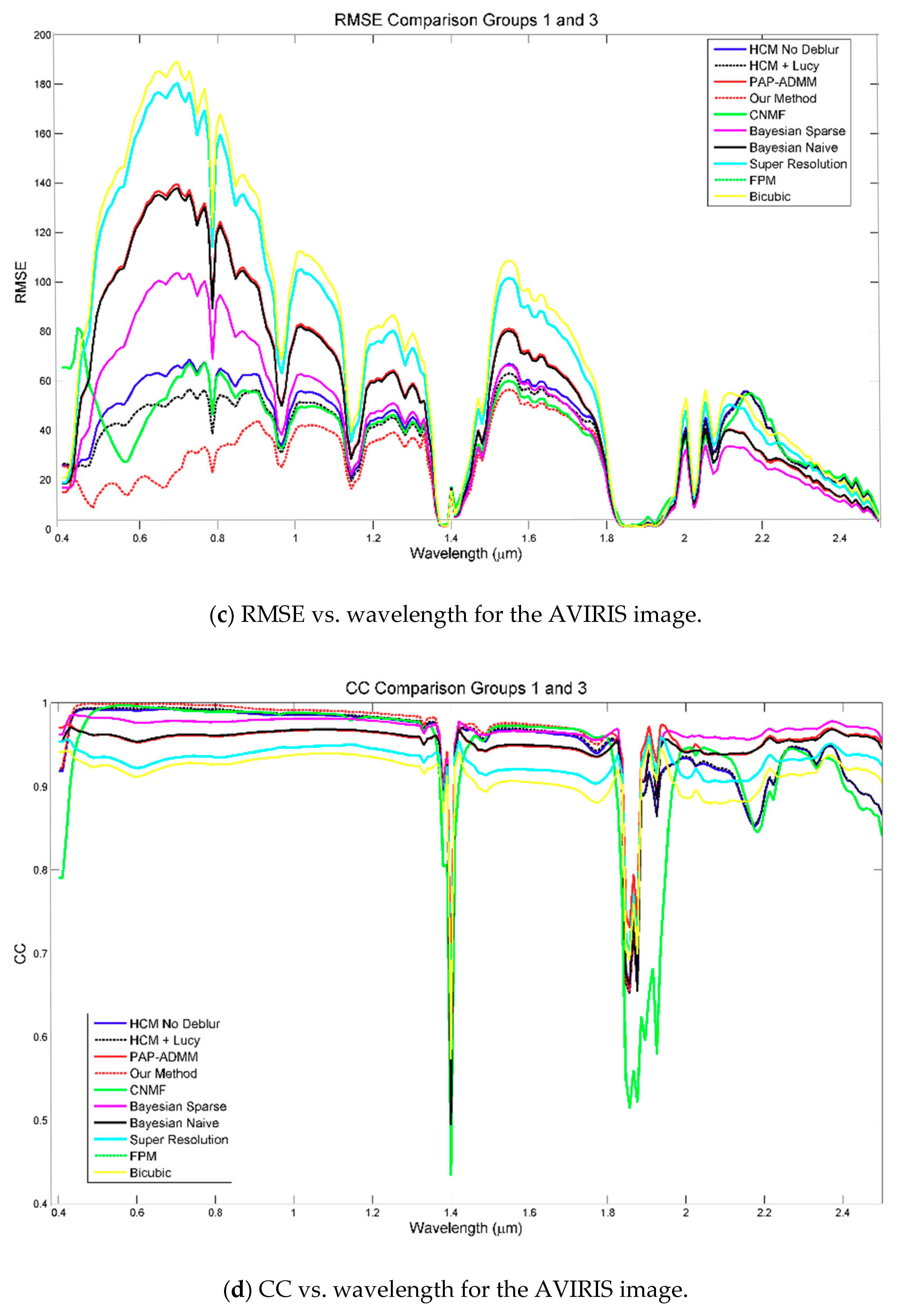
Figure 7.
Comparison of RMSE and CC between our method and methods in Group 4.
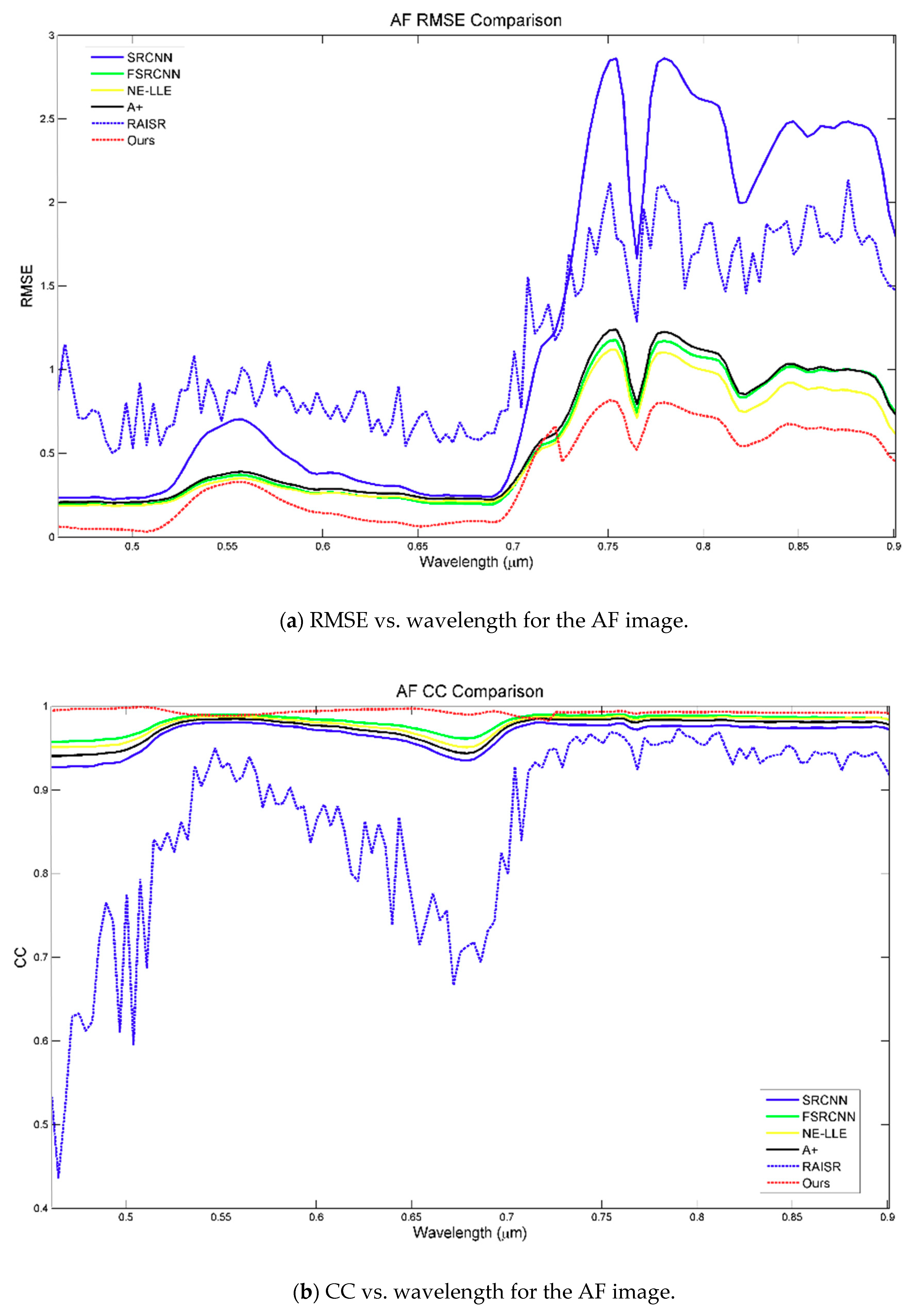

Figure 8.
Fused AF images using different methods. (a) Visible range and (b) VNIR range.
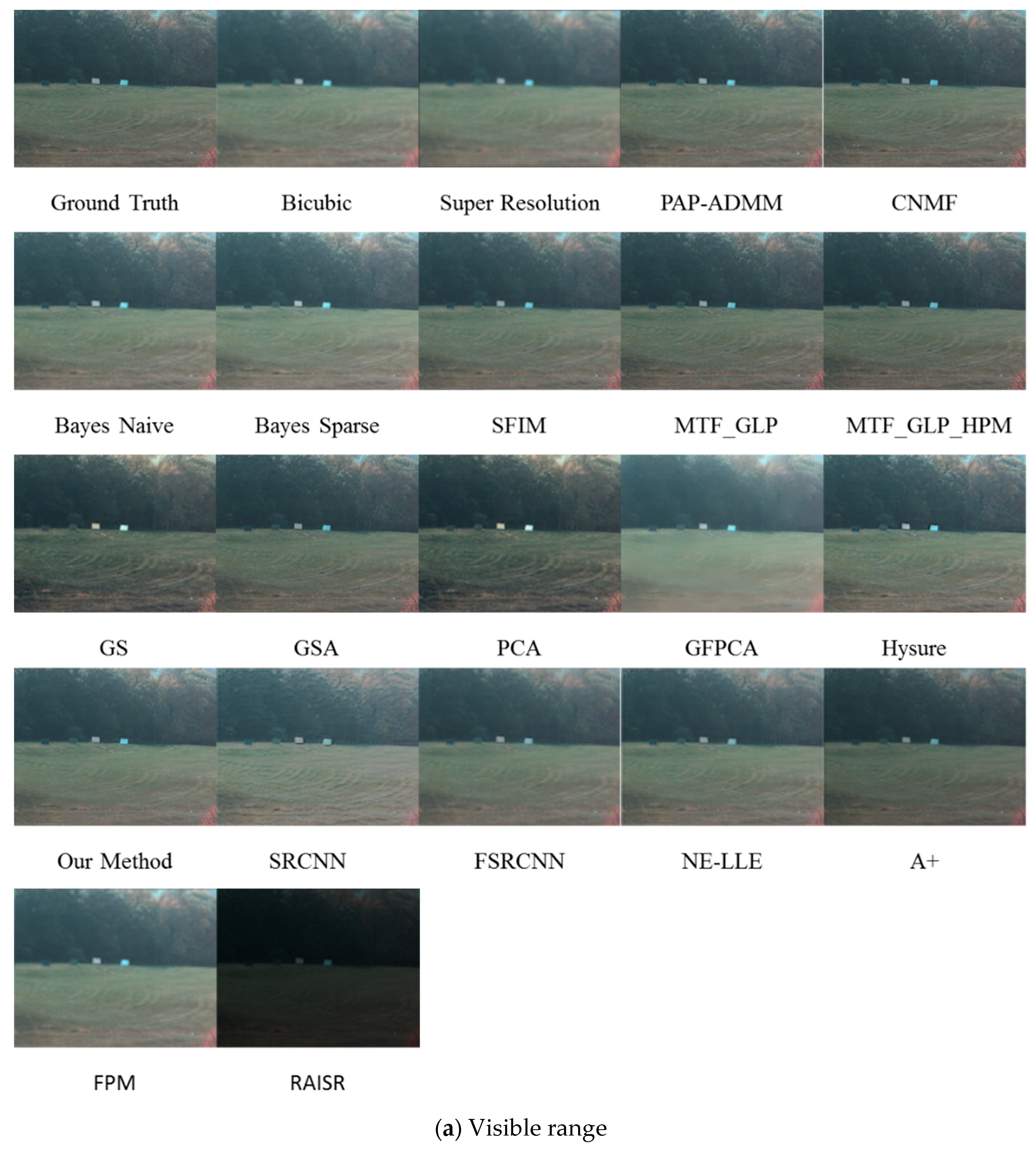
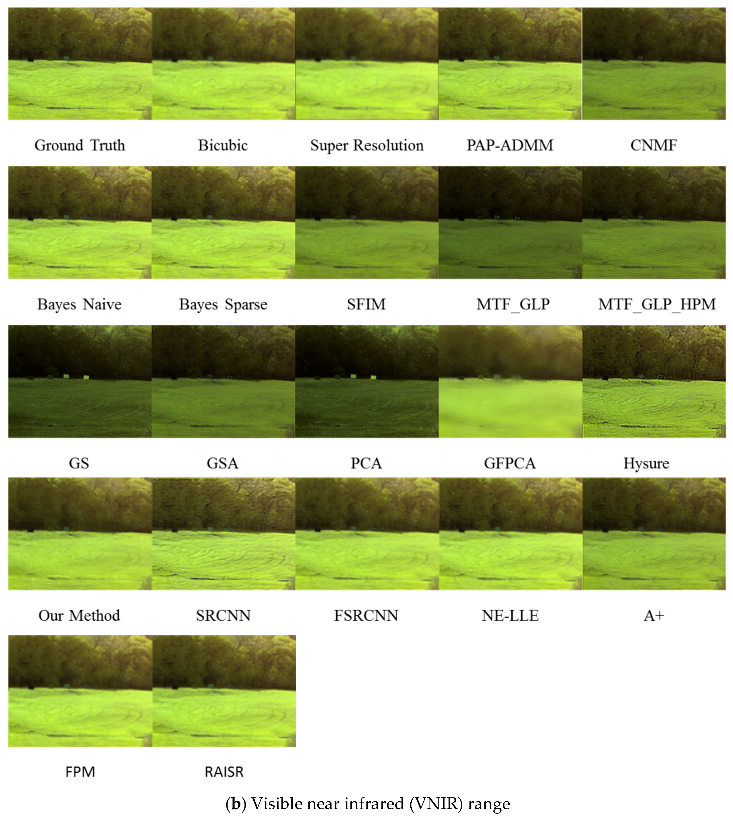
Figure 9.
Fused AVIRIS images using different methods. (a) Visible range, (b) VNIR range, and (c) SWIR range.
Figure 9.
Fused AVIRIS images using different methods. (a) Visible range, (b) VNIR range, and (c) SWIR range.
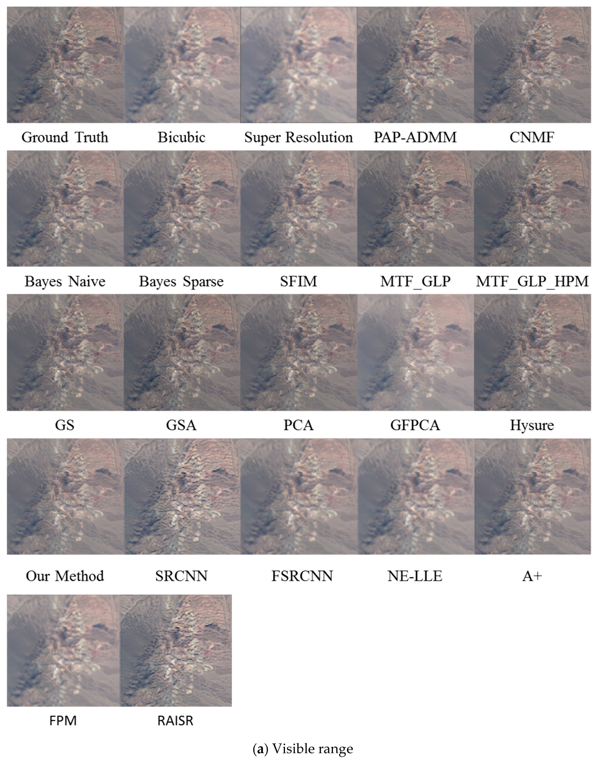


Figure 10.
Spectral signatures of the eight cluster centers.
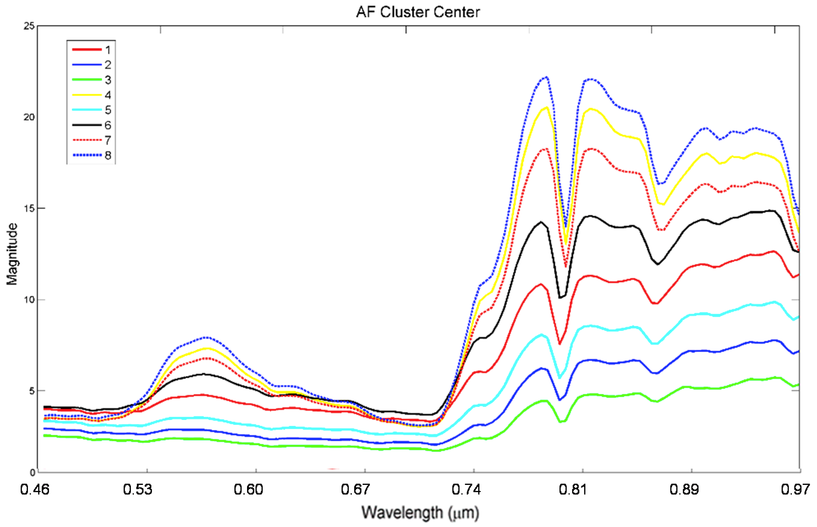
Figure 11.
Spectral signatures of the eight cluster centers.

Figure 12.
Pixel clustering accuracy using different algorithms for the AF dataset. Red: Group 1 methods; Blue: Group 2 methods; Green: Group 3 methods; Purple: HCM methods; Orange: Group 4 methods.
Figure 12.
Pixel clustering accuracy using different algorithms for the AF dataset. Red: Group 1 methods; Blue: Group 2 methods; Green: Group 3 methods; Purple: HCM methods; Orange: Group 4 methods.
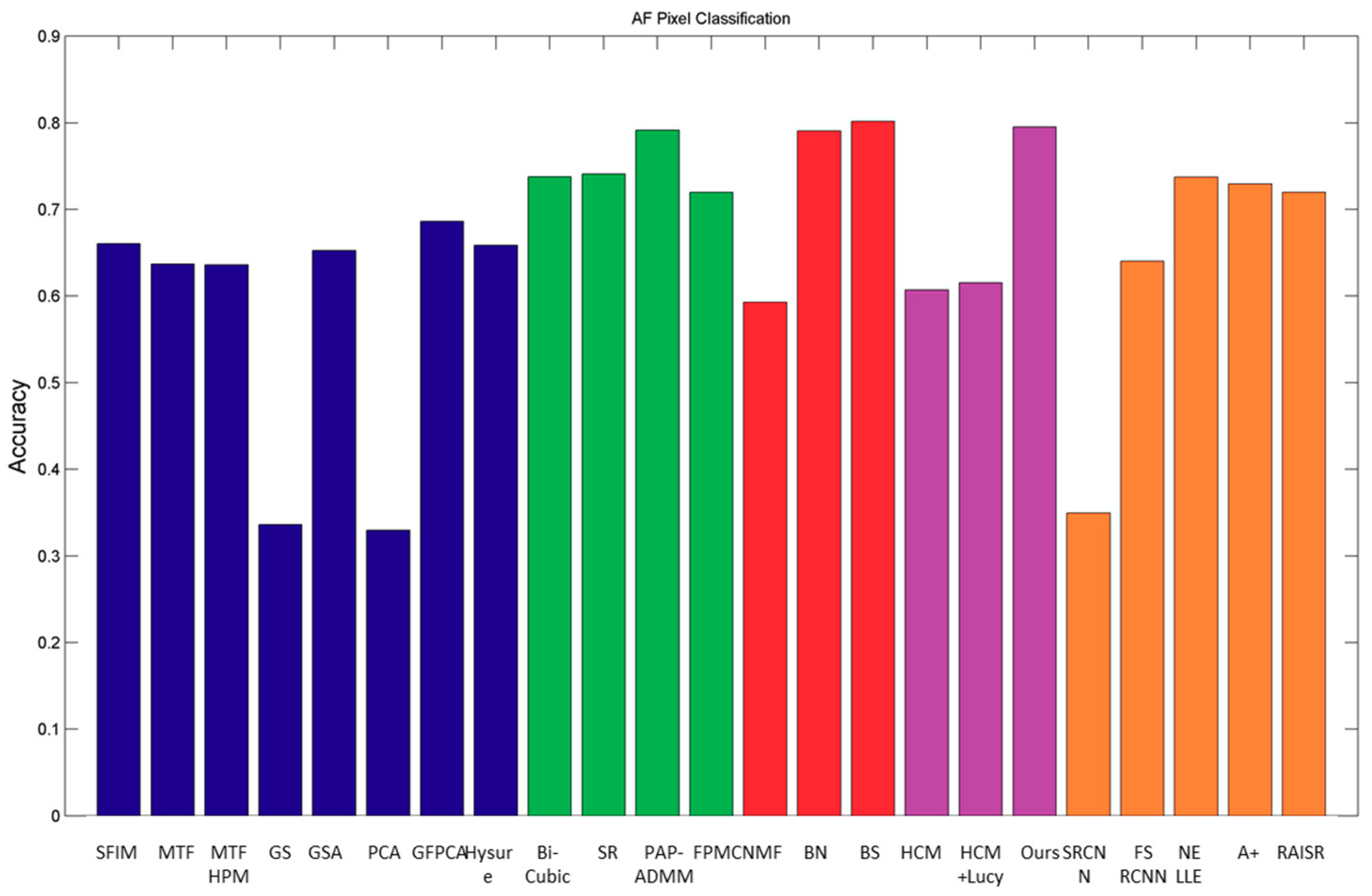
Figure 13.
Cluster maps of different algorithms for the AF data.

Figure 14.
Clustering accuracy using different algorithms for the AVIRIS dataset. Red: Group 1 methods; Blue: Group 2 methods; Green: Group 3 methods; Purple: HCM methods; Orange: Group 4 methods.
Figure 14.
Clustering accuracy using different algorithms for the AVIRIS dataset. Red: Group 1 methods; Blue: Group 2 methods; Green: Group 3 methods; Purple: HCM methods; Orange: Group 4 methods.

Figure 15.
Cluster maps of different algorithms for the AVIRIS data.


Table 1.
Comparison of various methods of HCM and PAP-ADMM on AVIRIS. Bold numbers indicate the best algorithm for each metric.
Table 1.
Comparison of various methods of HCM and PAP-ADMM on AVIRIS. Bold numbers indicate the best algorithm for each metric.
| Methods | RMSE | CC | SAM | ERGAS |
|---|---|---|---|---|
| PAP-ADMM [7] | 66.2481 | 0.9531 | 0.7848 | 1.9783 |
| HCM [8] | 44.3475 | 0.9492 | 0.9906 | 2.0302 |
| Proposed | 30.1907 | 0.9672 | 0.9008 | 1.7205 |
Table 2.
Comparison of our methods with various pansharpening methods on AF and AVIRIS. Bold numbers indicate best performers for each metric. Red numbers indicate second best methods.
Table 2.
Comparison of our methods with various pansharpening methods on AF and AVIRIS. Bold numbers indicate best performers for each metric. Red numbers indicate second best methods.
| AF | AVIRIS | ||||||||||
|---|---|---|---|---|---|---|---|---|---|---|---|
| Group | Methods | Time | RMSE | CC | SAM | ERGAS | Time | RMSE | CC | SAM | ERGAS |
| 1 | CNMF [9] | 12.5225 | 0.5992 | 0.9922 | 1.4351 | 1.7229 | 23.7472 | 32.2868 | 0.9456 | 0.9590 | 2.1225 |
| Bayes Naïve [10] | 0.5757 | 0.4357 | 0.9881 | 1.2141 | 1.6588 | 0.8607 | 67.2879 | 0.9474 | 0.8137 | 2.1078 | |
| Bayes Sparse [11] | 208.8200 | 0.4133 | 0.9900 | 1.2395 | 1.5529 | 235.4995 | 51.7010 | 0.9619 | 0.7635 | 1.8657 | |
| 2 | SFIM [20] | 0.9862 | 0.7176 | 0.9846 | 1.5014 | 2.2252 | 1.5615 | 63.7443 | 0.9469 | 0.9317 | 2.0790 |
| MTF GLP [16] | 1.3806 | 0.8220 | 0.9829 | 1.6173 | 2.4702 | 2.2464 | 57.5260 | 0.9524 | 0.9254 | 2.0103 | |
| MTF GLP HPM [17] | 1.3982 | 0.8096 | 0.9833 | 1.5540 | 2.4387 | 2.2250 | 57.5618 | 0.9524 | 0.9201 | 2.0119 | |
| GS [14] | 1.0496 | 2.1787 | 0.8578 | 2.4462 | 7.0827 | 1.8252 | 54.9411 | 0.9554 | 0.9420 | 1.9609 | |
| GSA [15] | 1.2079 | 0.7485 | 0.9875 | 1.5212 | 2.1898 | 1.9784 | 32.4501 | 0.9695 | 0.8608 | 1.6660 | |
| PCA [12] | 2.3697 | 2.3819 | 0.8382 | 2.6398 | 7.7194 | 2.9788 | 48.9916 | 0.9603 | 0.9246 | 1.8706 | |
| GFPCA [13] | 1.1724 | 0.6478 | 0.9862 | 1.5370 | 2.0573 | 2.1686 | 61.9038 | 0.9391 | 1.1720 | 2.2480 | |
| Hysure [18,19] | 117.0571 | 0.8683 | 0.9810 | 1.7741 | 2.6102 | 62.4685 | 38.8667 | 0.9590 | 1.0240 | 1.8667 | |
| 2* | SFIM [20] | 0.9743 | 0.6324 | 0.9901 | 1.3449 | 1.8881 | 1.5327 | 37.0572 | 0.9737 | 0.7205 | 1.5931 |
| MTF GLP [16] | 1.3482 | 0.7420 | 0.9882 | 1.4738 | 2.1628 | 2.1313 | 26.4199 | 0.9772 | 0.6975 | 1.5132 | |
| MTF GLP HPM [17] | 1.4132 | 0.7255 | 0.9887 | 1.4020 | 2.1171 | 2.1364 | 26.5246 | 0.9772 | 0.6969 | 1.5159 | |
| GS [14] | 1.0689 | 2.1660 | 0.8590 | 2.3500 | 7.0568 | 1.6384 | 54.1610 | 0.9624 | 0.8324 | 1.8748 | |
| GSA [15] | 1.2013 | 0.6572 | 0.9896 | 1.3541 | 1.9617 | 2.0012 | 42.8342 | 0.9698 | 0.7686 | 1.6734 | |
| PCA [12] | 2.3945 | 2.3755 | 0.8387 | 2.5490 | 7.7105 | 2.9703 | 48.0821 | 0.9680 | 0.8109 | 1.7678 | |
| GFPCA [13] | 1.1923 | 0.6754 | 0.9837 | 1.5688 | 2.1893 | 1.9354 | 73.6587 | 0.9362 | 1.2344 | 2.4518 | |
| Hysure [18,19] | 119.4377 | 0.8101 | 0.9832 | 1.6748 | 2.4467 | 66.0869 | 38.8677 | 0.9544 | 1.0355 | 1.9516 | |
| 3 | PAP-ADMM [7] | 21,440.000 | 0.4308 | 0.9889 | 1.1622 | 1.6149 | 3368.0000 | 66.2481 | 0.9531 | 0.7848 | 1.9783 |
| Super Resolution [21] | 279.1789 | 0.5232 | 0.9839 | 1.3215 | 1.9584 | 1329.5920 | 86.7154 | 0.9263 | 0.9970 | 2.4110 | |
| Bicubic [22] | 0.0412 | 0.5852 | 0.9807 | 1.3554 | 2.1560 | 0.1038 | 92.2143 | 0.9118 | 1.0369 | 2.5728 | |
| FPM [23] | 23.7484 | .5851 | 0.9804 | 1.3551 | 2.1555 | 52.63799 | 92.2141 | 0.9117 | 1.0369 | 2.5728 | |
| 4 | SRCNN [26] | 503.1755 | 1.5649 | 0.9663 | 2.8086 | 4.7609 | 4897.0460 | 303.9198 | 0.8291 | 1.5628 | 7.4368 |
| FSRCNN [27] | 470.0645 | 0.6637 | 0.9814 | 1.4091 | 2.3852 | 836.1380 | 109.2260 | 0.9052 | 1.0936 | 2.8898 | |
| NE+ LLE [25] | 27,848.000 | 0.6130 | 0.9779 | 1.4018 | 2.2859 | 44,722.000 | 92.3977 | 0.9106 | 1.0423 | 2.5791 | |
| A+ [24] | 40.5783 | 0.6872 | 0.9733 | 1.4156 | 2.5288 | 65.9070 | 100.9513 | 0.8925 | 1.0473 | 2.7643 | |
| RAISR [28] | 1287.2375 | 1.2830 | 0.8611 | 3.6061 | 6.0723 | 2341.1421 | 373.7005 | 0.3947 | 1.4193 | 13.0819 | |
| Ours | HCM no deblur [8] | 0.5900 | 0.5812 | 0.9908 | 1.4223 | 1.7510 | 1.5000 | 44.3474 | 0.9492 | 0.9906 | 2.0302 |
| HCM Lucy [46] | 1.2000 | 0.6009 | 0.9879 | 1.3950 | 1.9308 | 1.5000 | 37.2436 | 0.9518 | 0.9683 | 1.9720 | |
| Our method | 0.5900 | 0.4151 | 0.9956 | 1.1442 | 1.2514 | 1.5000 | 30.1907 | 0.9672 | 0.9008 | 1.7205 | |
© 2018 by the authors. Licensee MDPI, Basel, Switzerland. This article is an open access article distributed under the terms and conditions of the Creative Commons Attribution (CC BY) license (http://creativecommons.org/licenses/by/4.0/).
Share and Cite
MDPI and ACS Style
Kwan, C.; Choi, J.H.; Chan, S.H.; Zhou, J.; Budavari, B. A Super-Resolution and Fusion Approach to Enhancing Hyperspectral Images. Remote Sens. 2018, 10, 1416. https://doi.org/10.3390/rs10091416
AMA Style
Kwan C, Choi JH, Chan SH, Zhou J, Budavari B. A Super-Resolution and Fusion Approach to Enhancing Hyperspectral Images. Remote Sensing. 2018; 10(9):1416. https://doi.org/10.3390/rs10091416
Chicago/Turabian StyleKwan, Chiman, Joon Hee Choi, Stanley H. Chan, Jin Zhou, and Bence Budavari. 2018. "A Super-Resolution and Fusion Approach to Enhancing Hyperspectral Images" Remote Sensing 10, no. 9: 1416. https://doi.org/10.3390/rs10091416
Note that from the first issue of 2016, this journal uses article numbers instead of page numbers. See further details here.