Article

Hyperspectral Target Detection via Adaptive Information—Theoretic Metric Learning with Local Constraints

1
Hubei Subsurface Multi–Scale Imaging Key Laboratory, Institute of Geophysics and Geomatics, China University of Geosciences, Wuhan 430074, China
2
School of Computer, Wuhan University, Wuhan 430079, China
3
State Key Laboratory of Information Engineering in Surveying, Mapping, and Remote Sensing, Wuhan University, Wuhan 430079, China
*
Author to whom correspondence should be addressed.
Remote Sens. 2018, 10(9), 1415; https://doi.org/10.3390/rs10091415
Submission received: 18 July 2018 / Revised: 28 August 2018 / Accepted: 3 September 2018 / Published: 6 September 2018
(This article belongs to the Special Issue Dimensionality Reduction for Hyperspectral Imagery Analysis)

Abstract

:
By using the high spectral resolution, hyperspectral images (HSIs) provide significant information for target detection, which is of great interest in HSI processing. However, most classical target detection methods may only perform well based on certain assumptions. Simultaneously, using limited numbers of target samples and preserving the discriminative information is also a challenging problem in hyperspectral target detection. To overcome these shortcomings, this paper proposes a novel adaptive information-theoretic metric learning with local constraints (ITML-ALC) for hyperspectral target detection. The proposed method firstly uses the information-theoretic metric learning (ITML) method as the objective function for learning a Mahalanobis distance to separate similar and dissimilar point-pairs without certain assumptions, needing fewer adjusted parameters. Then, adaptively local constraints are applied to shrink the distances between samples of similar pairs and expand the distances between samples of dissimilar pairs. Finally, target detection decision can be made by considering both the threshold and the changes between the distances before and after metric learning. Experimental results demonstrate that the proposed method can obviously separate target samples from background ones and outperform both the state-of-the-art target detection algorithms and the other classical metric learning methods.

Graphical Abstract

1. Introduction

A hyperspectral image (HSI) obtained by remote sensing systems can provide significant information. Each pixel of HSI contains a continuous spectrum with hundreds or even thousands of spectral bands, of which the width of each band is about 5–10 nm, to detect and characterize target of interest in the scene [1,2]. Target detection is one of the most wide applications of hyperspectral image processing, and it plays an important role in the real world, such as detecting humanmade objects in reconnaissance applications, searching rare minerals in geology, and researching environmental pollution [3,4,5]. Based on specific spectral signatures (prior information), the purpose of target detection is to decide whether a target of interest is present or not present (background) in a pixel-under-test, which can be viewed as a binary classifier [6,7].
A number of classical target detection algorithms have been proposed in HSI analysis. Most of them are based on the linear models and statistical hypothesis tests, which can maximize the detection probability for fixed false alarm probability, such as orthogonal subspace projection (OSP) and adaptive cosine/coherence estimator (ACE). The former OSP method proposed by Harsanyi et al. [8] suppresses the background signatures by projecting each pixel’s spectrum onto a subspace, which is orthogonal to the background signatures. The well-known ACE method proposed by Kraut et al. [9] assumes that the additive noise has been included in background, which is an unstructured background detector. However, most classical algorithms depend on the specific statistical hypothesis tests, and may only perform well under certain conditions, e.g., the ACE detector assumes that the background is homogeneous, which is unrealistic in the real world.
In recent years, the machine learning techniques have been introduced into HSI target detection, which has been paid great attention [10,11]. Typical examples of these methods are kernel-based detectors, such as the kernel matched subspace detectors (KMSD) [12], kernel spectral matched filter (KSMF) [13], and kernel OSP [14]. The kernel-based methods map the original feature space into a potentially high-dimensional kernel space to solve the linearly inseparable problem in the original space. Apparently, as mentioned in the article [15], kernel-based methods are also based on statistical hypothesis test, and inherit the shortcomings of traditional target detection methods. It can be concluded that kernel-based methods attempt to find a stable and credible feature space (distance metric) for separating potential target pixels and background ones [16,17,18].
Otherwise, the spectral resolution of HSIs is so high that these spectral bands are often highly correlated. For decreasing spectral redundancy and releasing computational complexity, it is necessary to reduce dimension by discarding redundant features for HSI target detection [19,20]. There are such few target pixels of interest that HSI target detection rarely takes into consideration dimensionality reduction, which may hide the accuracy of detecting targets. That is to say, target detection is usually in a dilemma whether to reduce spectral redundancy or preserve discriminative information [21,22]. Thus, how to develop a proper metric with a low dimensionality for measuring the separability between target pixels and background ones becomes the key for HSI target detection [23].
In fact, metric learning methods have proved to be a more straightforward and effective way to obtain such a distance metric [24,25,26]. To date, there are a few metric learning methods that have been proposed for HSI target detection. For example, Zhang et al. [15] learned an objective function of the supervised distance maximization by putting a similarity propagation constraint and imposing a manifold smoothness regularization. Dong et al. [27] presented the maximum margin metric learning (MMML) method, which utilizes the maximum margin framework as the objective function to learn distance metric space and can maximally separate target samples from background ones without certain assumptions. Dong et al. [28] presented random forest metric learning (RFML) method, which adopts random forests as the underlying representation of the metric learning, to deal with limited numbers of target samples by merging the standard relative position and the absolute pairwise position. In general, by using metric learning, we can find the distance metric matrix, so as to transform the original space into the metric feature space. Then, we can detect the desired targets, especially when the samples are imbalanced and the number of target samples is very limited.
In addition, a number of metric learning methods have been proposed to learn the distance metric, such as neighborhood component analysis (NCA) method [29], large margin nearest neighbor (LMNN) method [30], and so on. For each instance, NCA method expresses the probability of selecting the same class instances as the neighbors, which can maximize the stochastic variance of leave-one-out k-nearest neighbor (KNN) score on the training samples. LMNN method aims to find a distance metric such that the instances from different classes are effectively separated by a large margin within the neighborhood, where the margin is defined as the difference between the between-class and within-class distances. Furthermore, the information-theoretic metric learning (ITML) method, proposed by Davis et al. [31], expresses the weakly supervised metric learning problem as a Bregman optimization problem and can handle a variety of constraints and incorporate a priori information on the distance function.
However, the existing metric learning based methods still have some obstacles to be addressed. The major problem is that most methods mentioned above are global metric learning with global constraints, making decisions by comparing their Mahalanobis distance d and judging d is lower or higher than the a fixed threshold b, which is insufficient and suboptimal. Therefore, in this paper, ITML method, which works in a weakly supervised manner, is innovatively introduced for hyperspectral target detection with adaptively local constraints (ITML-ALC, for short). The proposed ITML-ALC method explores adaptively local constraints to relax the fixed threshold, which can be used to compute the Mahalanobis distance d and judge if given samples are targets by considering both b and the changes between the distances before and after metric learning. By considering local constraints and avoiding adopting those conflicting constraints, the separability between target samples and background ones can be enhanced. Besides, non-square matrix W can be found for handling high-dimensional data problems by transforming the original space into a metric learning space with a low dimensionality. Compared with existing algorithms, ITML-ALC has several obvious advantages:
  • The proposed ITML-ALC algorithm can use limited numbers of target samples to detect targets without certain assumptions, compared with traditional target detection methods.
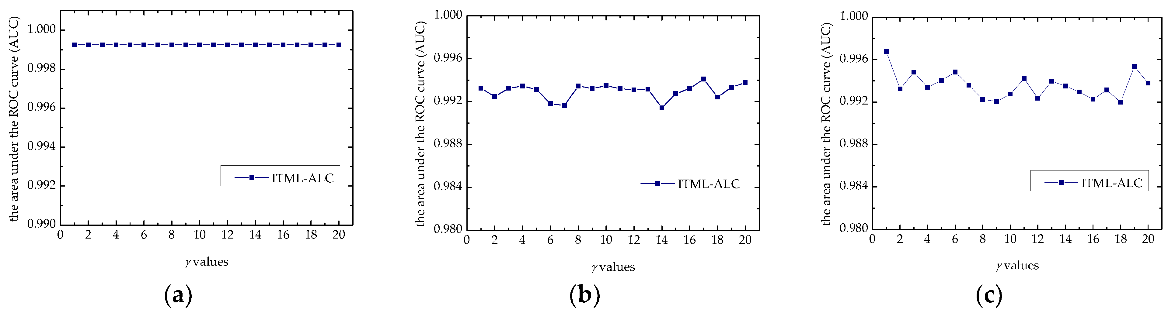
  • ITML-ALC needs only one parameter to be adjusted, and the detection results are relatively stable for different values of parameter.
  • ITML-ALC can remain the locality information and improve the detection performance via considering both the threshold and the changes between the distances before and after metric learning, while existing metric learning based methods uses fixed threshold to make decision.
The rest of this paper is organized as follows. In Section 2, a briefly introduce of the original ITML method is provided, and the proposed ITML-ALC method is then presented. The experimental results of the proposed method using several challenging HSIs are detailed in Section 3, followed by the discussion and conclusions in Section 4 and Section 5.

2. Methods

2.1. Related Work

The ITML methodology minimizes the LogDet divergence subject to linear constraints. There are two key techniques of ITML. One is the ability to handle a wide variety of constraints and to optionally incorporate a priori information on the distance function. The other key technique is that it is fast and scalable.
Suppose that we have a set of L-dimensional training samples { x 1 , x 2 , , x n } R L × n , in which n represents the number of training samples and L is the number of feature dimensions. z i j ( + 1 , 1 ) denotes the relationship between the training samples x i and x j . Considering relationships of the similarity or dissimilarity between pairs of samples, distances between samples in the same class can be constrained as similar, and ones in different classes can be constrained as dissimilar. Then, we have a set of similar constraints S and a set of dissimilar constraints D as Equation (1):
S : ( x i , x j ) S x i , x j same   class ,   z i j = 1 , D : ( x i , x j ) D x i , x j different   class ,   z i j = 1 .
Metric learning aims to learn metric matrix M , which specifies the Mahalanobis distance d M ( x i , x j ) between any pairs of samples x i and x j as:
d M ( x i , x j ) = ( x i x j ) T M ( x i x j ) .
In order to ensure that d M ( x i , x j ) is a meaningful distance, the learned metric matrix M must be symmetric and positive semidefinite (PSD) variance matrix, guaranteeing that d M ( x i , x j ) is symmetrical, non-negativite, and has triangle inequality [32,33]. Considering the high dimensional of HSIs and M is PSD matrix, a nonsquare matrix W R L × D ( D L ) , defining a mapping from the high-dimensional space into a low-dimensional embedding, can be established, and M = W W T [34,35,36].
In the Equation (2), our objective is to find the PSD matrix M (or W ) and the corresponding distance threshold b such that for any pairs ( x i , x j ) S the distance between them is smaller than b, and for any pairs ( x i , x j ) D the distance between them is greater than b, which can be described as Equation (3):
d M ( x i , x j ) b ( x i , x j ) S , d M ( x i , x j ) b ( x i , x j ) D .
The ITML method can minimize the differential relative entropy between two multivariate Gaussians and handle a variety of constraints on the distance function via a natural information-theoretic approach. Thus, given a Mahalanobis distance parameterized by M , its corresponding multivariate Gaussian can be expressed as:
p ( x ; M ) = 1 Z exp ( 1 2 d M ( x , μ ) ) ,
where μ is the mean of Gaussians, Z is a normalizing constant in the Equation (4). By using the bijection, the distance between two Mahalanobis distance functions parameterized by M 0 and M can be measured by the differential relative entropy of corresponding multivariate Gaussians:
KL ( p ( x ; M 0 ) | | p ( x ; M ) ) = p ( x ; M 0 ) log p ( x ; M 0 ) p ( x ; M ) dx ,
In the Equation (5), M 0 is a given Mahalanobis distance function, such as identity matrix. In conjunction with given pairs of similar points S and pairs of dissimilar points D , the distance metric learning can be summarized as the following optimization problems:
min M KL ( p ( x ; M 0 ) | | p ( x ; M ) ) subject   to   d M ( x i , x j ) b 1     ( x i , x j ) S , d M ( x i , x j ) b 2     ( x i , x j ) D ,
where b 1 , b 2 are given upper and lower bounds, respectively.
Some research has shown that the differential relative entropy of corresponding multivariate Gaussians is equivalent to the LogDet divergence between the covariance matrices [37]:
KL ( p ( x ; M 0 ) | | p ( x ; M ) ) = 1 2 d log det ( M 0 1 , M 1 ) = 1 2 d log det ( M , M 0 ) ,  
where M 0 1 , M 1 are the covariance of the distributions.
Taking into account that a feasible solution of Equation (6) may not exist, we incorporate slack variable ξ into Equation (6) to guarantee the existence of the metric matrix M . Thus, the Equation (6) can be represented as the following optimization problem with Equation (7):
min M 0 , ξ d log det ( M , M 0 ) + γ · d log det ( diag ( ξ ) , diag ( ξ 0 ) ) s . t .   tr ( M ( x i x j ) ( x i x j ) T ) ξ c ( i , j )   ( x i , x j ) S ,    tr ( M ( x i x j ) ( x i x j ) T ) ξ c ( i , j )   ( x i , x j ) D ,
where ξ 0 denotes initialized slack variables, and c ( i , j ) is the index of the ( i , j ) th constraint. γ is the tradeoff parameter, which controls the tradeoff between satisfying the constraints and minimizing d log det .

2.2. Combining ITML and Adaptively Local Constraints

The ITML method uses fixed threshold to make decision, which makes it less effective to handle data with complex distributions even if the associated metric is correct. To address this issue, this paper proposes an adaptively local decision rule to design pairwise constraints to relax the fixed threshold for target detection. We design a local decision function f ( d i j ) to achieve this goal, where d i j is the distance of a similar or dissimilar pair ( x i , x j ) . The principle for designing f ( d i j ) is: that the greater the distance between similar pairs, the more f ( d i j ) should shrink, while the smaller the distance between dissimilar pairs, the more f ( d i j ) should expand. Based on this principle, the local constraints can be redefined to make better decision by considering both the threshold b and the changes between the distances before and after metric learning. As a result, we can form the local decision constraints to compute the adaptive upper/lower bounds for ( x i , x j ) as:
f S ( d i j ) = d i j ( d i j ( 1 / N S ) / d c ) ( x i , x j ) S , f D ( d i j ) = d i j + ( d c / d i j ( 1 / N D ) ) ( x i , x j ) D ,
where N S 1 and N D 1 are the scale factors that separately control shrinkage and expansion. d c 1 is the constant.
From Equation (9), we can see that the smaller the N S is, the faster f S ( d i j ) will shrink, while the greater the N D is, the faster f D ( d i j ) will expand. Then we set d c = d m a x (where d m a x is the maximal distance between all the pairs). Clearly, we want to maximize the shrinkage and expansion of f ( d i j ) . Considering that N S 1 cannot guarantee that the constraints are positive, we set N S = 1 to ensure that f S ( d i j ) can shrink as fast as possible, while setting N D = 1 / log 2 ( d c / ( d c 2 ) ) to guarantee the faster expansion of f D ( d i j ) . Thus, Equation (9) can be transformed as:
f S ( d i j ) = d i j ( d i j / d max ) ( x i , x j ) S , f D ( d i j ) = d i j + ( d max / d i j N D ) ( x i , x j ) D ,
For relaxing the fixed threshold of ITML method in the Equation (8), we can substitute the original fixed bound of ITML with the above-mentioned local decision constraints of Equation (10), and we finally obtain the adaptive ITML with local constraints (ITML-ALC) detector:
min M 0 , ξ d log det ( M , M 0 ) + γ d log det ( diag ( ξ ) , diag ( ξ 0 ) ) s . t .   d M ( x i , x j ) f S ( d M ( x i , x j ) ) + ξ c ( i , j )   ( x i , x j ) S ,    d M ( x i , x j ) f D ( d M ( x i , x j ) ) + ξ c ( i , j )   ( x i , x j ) D ,    ξ c ( i , j ) 0 ,   ( i , j ) ,   d 0 ,
In addition, combining Equation (1) with Equation (11), we can set the following Equation (12):
f ( d i j , z i j ) = { f S ( d M ( x i , x j ) ) x i , x j same   class , z i j = 1 , f D ( d M ( x i , x j ) ) x i , x j different   class , z i j = 1 .
Thus, the final ITML-ALC objective function can be simplified as:
min M 0 , ξ d log det ( M , M 0 ) + γ d log det ( diag ( ξ ) , diag ( ξ 0 ) ) s . t .   z i j d M ( x i , x j ) f ( d i j , y i j ) + ξ c ( i , j )    ξ c ( i , j ) 0 ,   ( i , j ) ,   M 0 ,
Obviously, ITML-ALC has the same complexity and can be solved using the same algorithm as ITML.

2.3. Final Sketch of ITML-ALC Algorithm

In the Equation (13), the metric matrix M can be projected into the PSD cone by adopting spectral decomposition. To compute the linear projections, we solve the following generalized eigenvector problem as:
M = i = 1 m λ i ν i T ν i
In the Equation (14), we start with setting the negative eigenvalues λ to zero, then we can obtain metric matrix M by using the remaining positive eigenvalues and the corresponding eigenvectors ν . Then, we can further learn a linear projection matrix W R L × D ( D L ) for the dimensionality reduction. For an arbitrary test pixel vector x i R L × n , we compute the final metric feature representation in the final ITML-ALC feature space with the equation M = W W T by:
x = W T x
By applying Equation (15), the original data x can be transformed into the Mahalanobis metric space. Finally, the target detection result is obtained by using a detection algorithm. In our method, the ACE detector is used because of its simplicity and effectivity.
Algorithm 1: Procedure of ITML-ALC
Input: A set of pairwise training data points { ( x i , x j , z i j ) ( S D ) } , the trade–off parameter γ
Output: Metric matrix M
Step (1): Initialization: input Mahalanobis matrix M 0 = I , initialized slack variable ξ 0 , d c = d m a x , N S = 1 ,
N D = 1 / log 2 ( d c / ( d c 2 ) ) .
Set: M = M 0 , λ i j = 0 . { ξ c ( i , j ) f S ( d i j ) , ( x i , x j ) S ξ c ( i , j ) f D ( d i j ) , ( x i , x j ) D
Step (2): Repeat {Main loop}
(a) p ( x i x j ) T M ( x i x j )
(b) α min ( λ i j , z i j 2 ( 1 p γ ξ c ( i , j ) ) ) , { z i j = 1 , ( x i , x j ) S z i j = 1 , ( x i , x j ) D
(c) β z i j α / ( 1 z i j α p )
(d) ξ c ( i , j ) γ ξ c ( i , j ) / ( γ + z i j α ξ c ( i , j ) )
(e) λ i j λ i j α
(f) M M + β M ( x i x j ) T ( x i x j ) M
Until: convergence is attained
Return: M
The proposed ITML-ALC algorithm is the integration of the ITML method and adaptively local constraints. Thus, ITML-ALC can be solved by using the same algorithm as the procedure of ITML. Refer to the reference [31], and we can obtain the procedure of the proposed ITML-ALC algorithm, summarized as Algorithm 1.

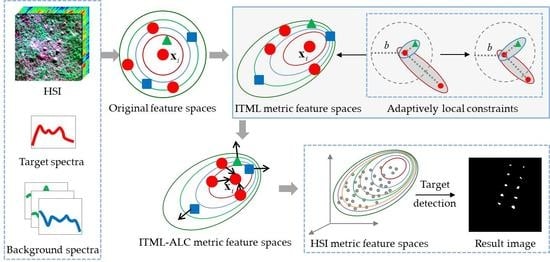
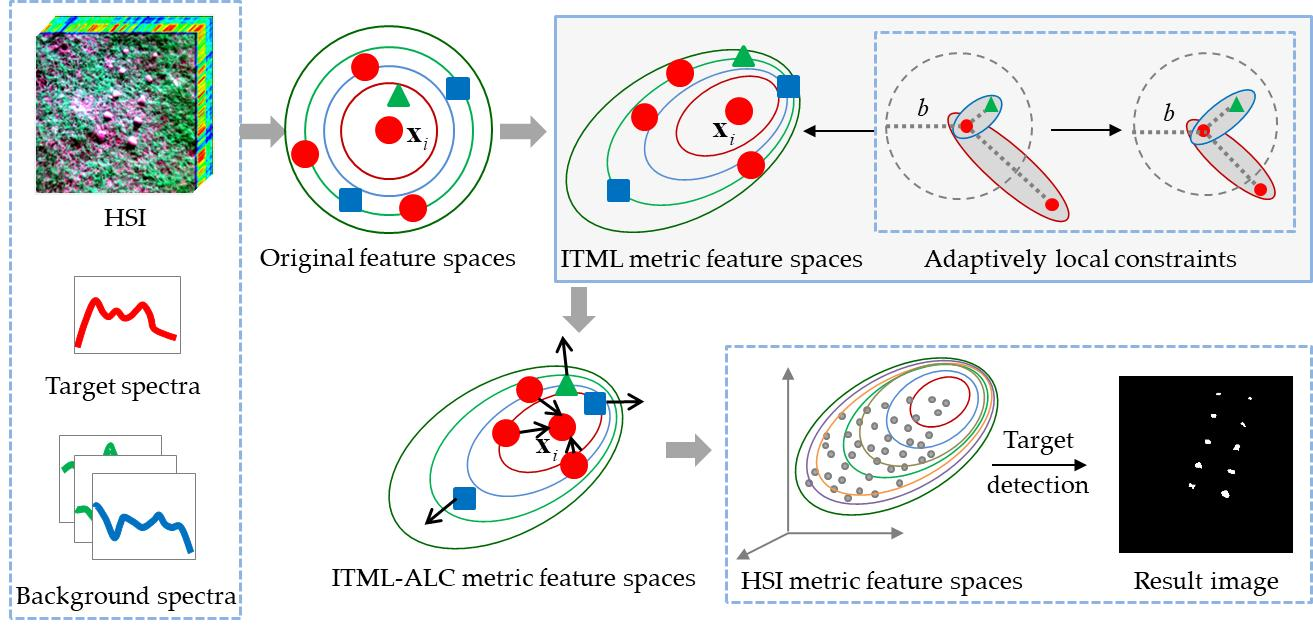
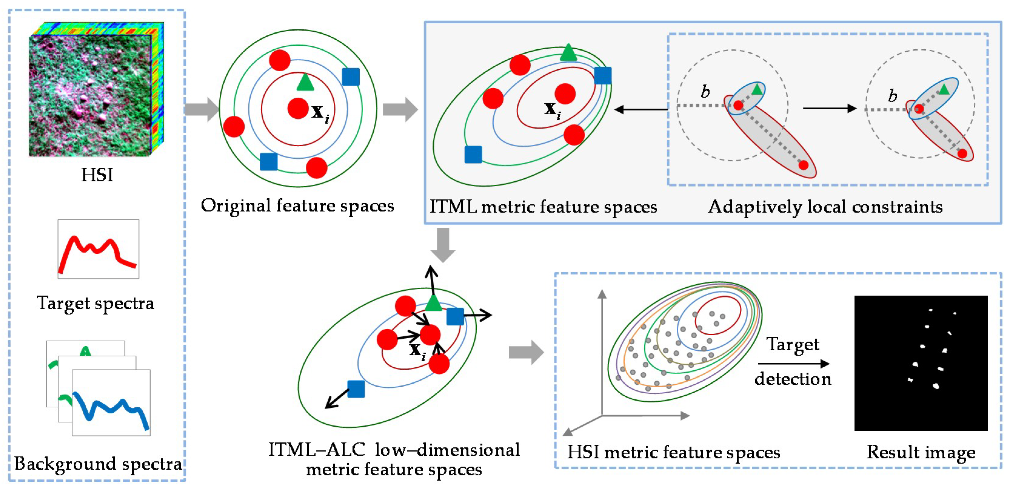
2.4. Workflow of ITML-ALC Algorithm

The schematic diagram of the proposed ITML-ALC method for HSI target detection is shown in Figure 1. Given a hyperspectral image, a priori information of the ITML-ALC algorithm including target samples (red points) and background samples (green points and blue points) is needed. The flowchart of the proposed algorithm consists of the following steps: (1) The ITML metric feature framework is constructed, which can transform the original HSI data into the Mahalanobis metric space. (2) The adaptively local decision constraints are applied into ITML framework. Unlike the fixed decision paradigm, which may be easily misclassified, we can classify the pairs according to the adaptively local decision constraints, with which the distance of the similar pair shrinks while the distance of the dissimilar pair expands as much as possible, illustrated in the solid box. Thus, it allows us to make a correct decision by considering both the threshold b and the changes between the distances before and after metric learning. (3) For achieving target detection, we transform the original HSI data into the ITML-ALC low-dimensional metric feature space, in which target samples can be maximally separated from the background ones. (4) We apply the specific detector to obtain the target detection results.

3. Experiments Analysis and Results

In this section, a synthetic dataset and two real datasets are performed to evaluate the effectiveness of the proposed method. The first one is a synthetic HSI dataset created through implanting alunite object spectra into the specific locations. The second and third ones are real HSI datasets with complex background distributions. For comparison, a series of existing state-of-the-art target detection algorithms, i.e., ACE and OSP detectors, are used to thoroughly evaluate the performance of the proposed algorithm. We also compare the proposed algorithm with three classical metric learning methods, i.e., LMNN, NCA, and ITML, which can also be applied to dimensionality reduction. In all the detectors (except ACE), we apply the same given training samples, including the target signatures and background signatures, which are randomly selected from the datasets. For ACE algorithm, we only implement the same target signatures as the proposed algorithm. In addition, we apply the ACE detector as the basic detector in the LMNN, NCA, and ITML algorithms like the proposed algorithm. As for the adjustment of parameters, trade-off parameters in the LMNN, NCA and ITML algorithms are tuned via threefold cross validation according to relative references [30], [29], and [31], respectively. All the experiments are implemented on a computer with an Intel(R) Core(TM) i7-7700 Central Processing Unit (CPU) at 3.60 GHz (8 GPUs), 16-GB Random Access Memory (RAM) and 64-bit Windows 10 Operating System (OS).

3.1. Dataset Description

Three hyperspectral datasets were used in this study to evaluate the performance of the proposed method introduced in Section 3.
(1)
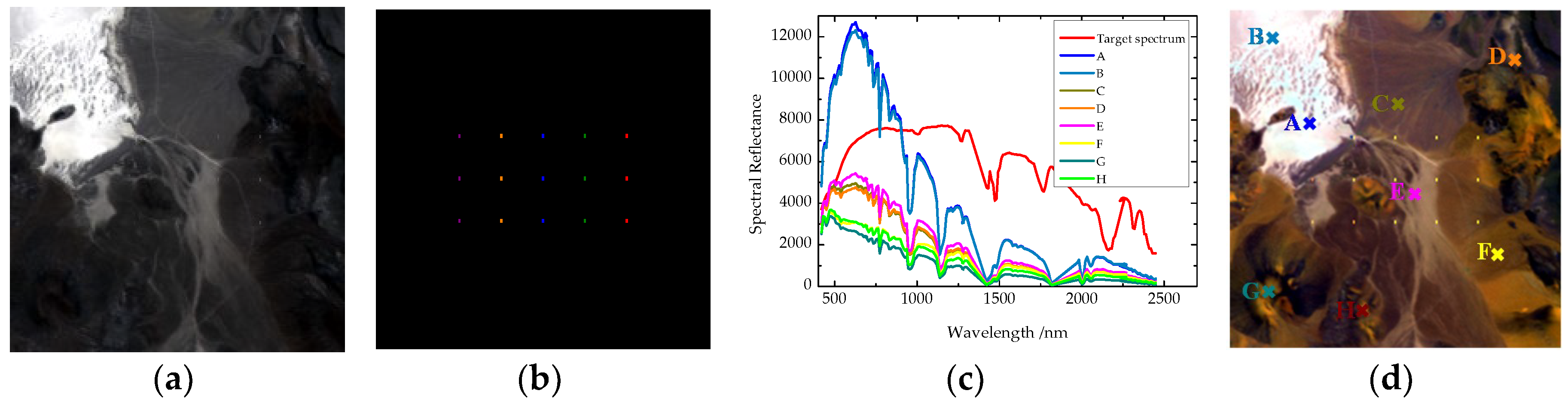
AVIRIS LCVF dataset: This image was acquired by the Airborne Visible/Infrared Imaging Spectrometer (AVIRIS) sensor, operated by National Aeronautics and Space Administration (NASA), USA, covering the Lunar Crater Volcanic Field (LCVF) in Northern Nye County, NV, USA. This dataset is a synthetic dataset and is available from the website of NASA website. Many studies used this dataset for HSI processing [38,39]. The spatial resolution of the LCVF image is 20 m per pixel, and the spectral resolution of the image is 5 nm, with 224 spectral channels in wavelengths ranging from 370 to 2510 nm. An area of 200 × 200 pixels is used for the experiments, as shown in Figure 2a, including red oxidized basaltic cinders, rhyolite, playa (dry lakebed), shade, and vegetation. We implant the alunite spectrum, which is obtained from the U.S. Geological Survey (USGS) digital spectral library, into the image for simulating target detection in the considered scene. Figure 2b shows corresponding locations of the implanted target panels. The added target panels have the same size, i.e., two pixels for each target panel, and the detailed coordinates of all 30 target pixels are given in Table 1. In this table, all the implanted target pixels are mixed pixels, and each spectrum x of the HSI is mixed with the pure prior target spectrum t and the original background spectra b by the following equation: x = p t + ( 1 p ) b , where p is the implanted fraction, which varies from 10% to 50%, as indicated in Table 1. The adopted pure target spectrum and some representative background samples spectra (denoted as A to H) are shown in Figure 2c, and the locations of the background samples given in Figure 2c are highlighted in Figure 2d.
(2)
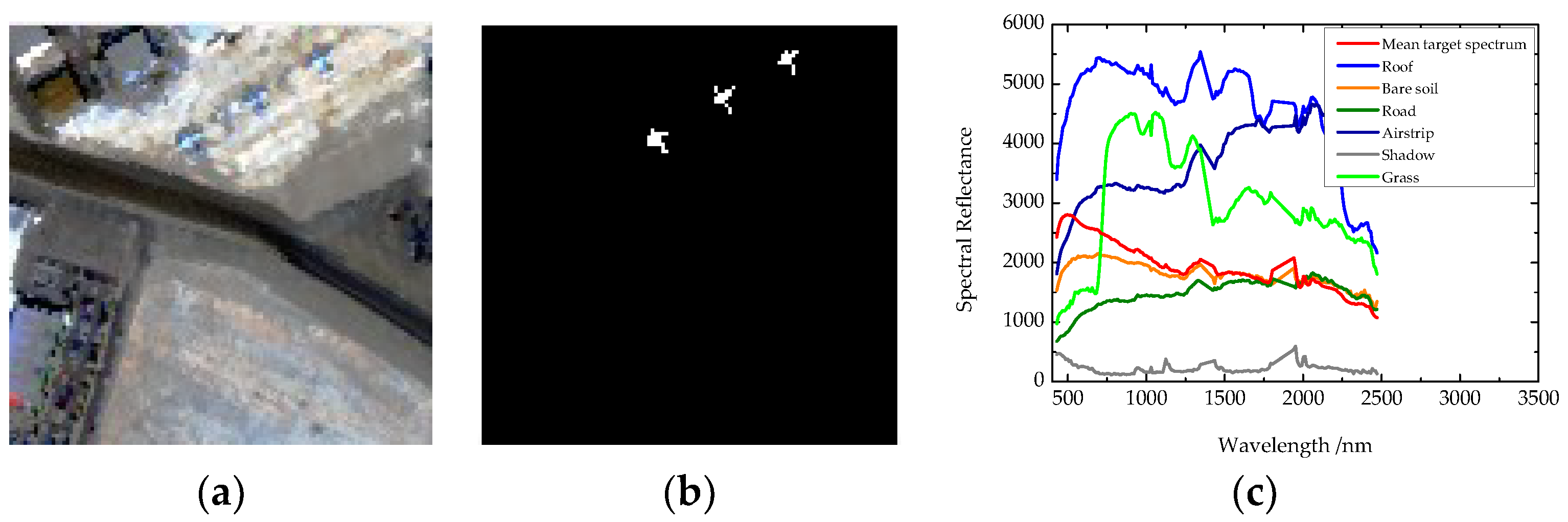
AVIRIS San Diego airport dataset: This image capturing an airport in the region of San Diego, CA, USA, was recorded by the AVIRIS sensor, as shown in Figure 3a [40]. The spatial resolution of this image is 3.5 m per pixel. The image has 224 spectral channels in wavelengths ranging from 370 to 2510 nm. A total of 189 bands are used in the experiments after removing the bands that correspond to the water absorption regions, low-signal noise ratio (SNR), and bad bands (1–6, 33–35, 97, 107–113, 153–166, and 221–224). An area of 100 × 100 pixels is used for the experiments, including roofs, bare soil, grass, road, airstrip, and shadow, which contains more complicated background land-cover classes. There are three airplanes in the image denoted as the targets of interest, which consist of 58 target pixels, and are denoted with the white target mask in Figure 3b. Figure 3c shows the spectra of mean target pixels and some representative background samples. We select the target spectra of the centers of airplanes as a priori target spectra, and we randomly select eight background spectra as the background samples.
(3)
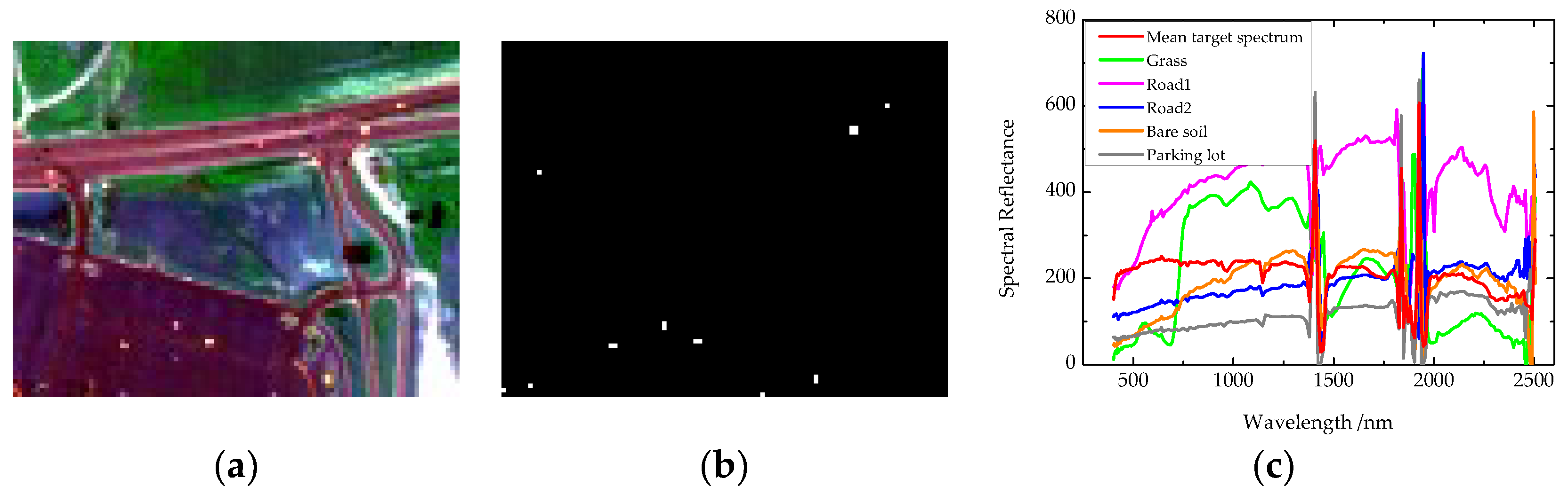
HYDICE urban dataset: This image is a Hyperspectral Digital Imagery Collection Experiment (HYDICE) airborne sensor dataset, sponsored by the U.S. Navy Space and Warfare Systems Command, covering a suburban residential area [41,42], as illustrated in Figure 4a. The scene mainly covers grass fields with some forest, and the rest of the scene is mixed with a parking lot with some vehicles, a residential area, and a roadway where some vehicles exist. The spatial resolution of this image is approximately 3 m, and the spectral resolution of the image is about 10 nm. The image scene contains an area of 80 × 100 pixels, with 210 spectral bands in wavelengths ranging from 400 to 2500 nm. There are 17 pixels of desired targets, the vehicles, which are contained in the parking lot and the road, as shown in Figure 4b. Besides, the spectra of mean target pixels and some representative background samples are illustrated in Figure 4c. We randomly select a target spectrum as a priori target spectrum, and seven background spectra as the background samples.
Taken together, we summary the details of experimental images acquired from different sensors, illustrated in Table 2.

3.2. Parameter Analysis

In this subsection, we evaluate the effect of the parameters on the detection performance of the proposed ITML-ALC algorithm. Similar to LMNN, NCA and ITML, the proposed algorithm also has a trade-off parameter, i.e., γ , which can be tuned via threefold cross validation. However, according to experimental studies, it can be observed that the AUCs of different γ values are relatively stable, which inspired us to set γ = 1 for all the experiments, illustrated in Figure 5.

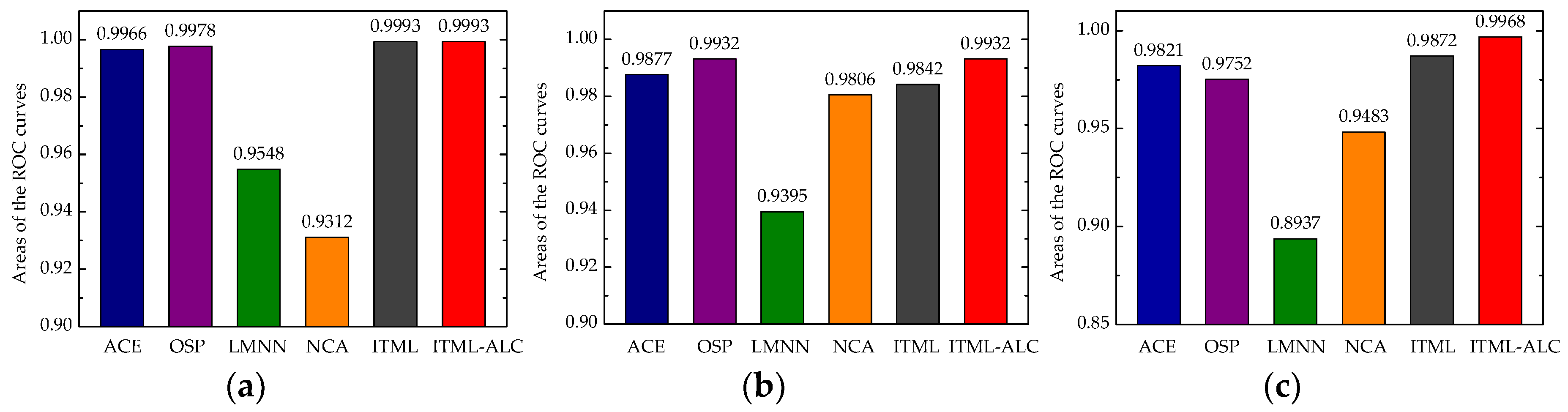
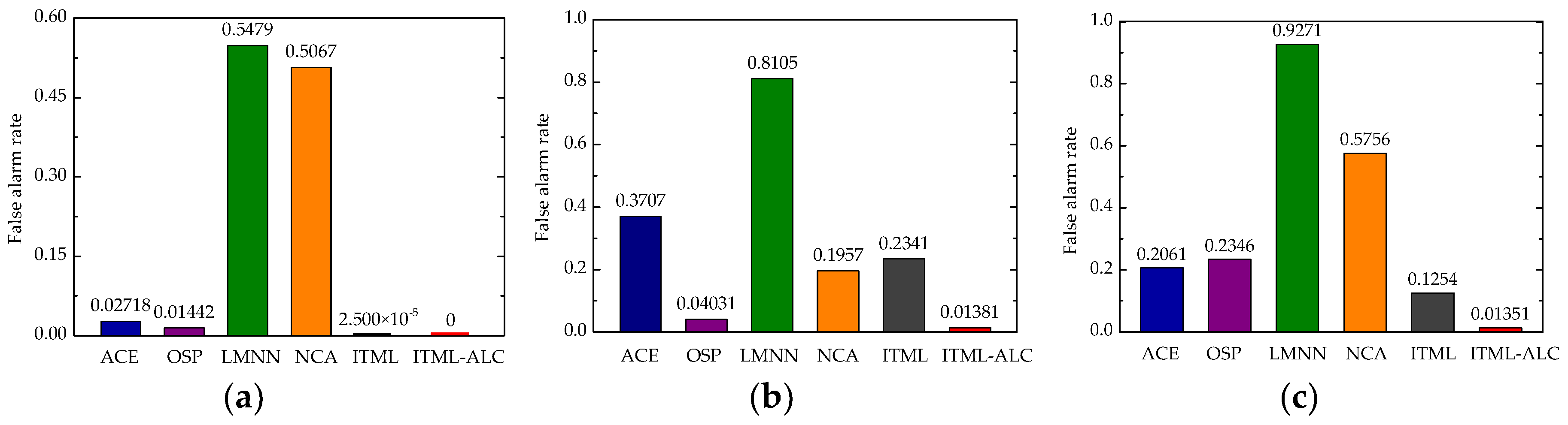
3.3. Detection Results and Validation

In this subsection, the detection performance of the proposed ITML-ALC algorithm is evaluated quantitatively by receiver operating characteristic (ROC) curves and target-background separation maps [1,8]. ROC curves are widely used as a standard performance evaluation tool for target detection applications, which can describe the relationship between the detection probability (the ratio of the number of corrected-detected target pixels to the total number of target pixels in the image) and false alarm rate (FAR, the ratio of the number of background pixels mistaken as targets to the total number of pixels in the image) based on the ground truth. Obviously, for the same level of FAR, the algorithm with the highest detection performs better, which locates further near the top left of the coordinate plane. Target-background separation maps can intuitively show how the target pixels are separated from the background ones. Generally speaking, good detector may highlight the targets and suppress the background into a small range of values while distinguishing the targets. Moreover, we can also consider the area under the ROC curve (AUC) to assess the accuracy, obtaining the average behavior [43]. Meanwhile, we use the FAR under TDR = 100% to further evaluate the detection performance [44].
For the AVIRIS LCVF dataset, the two-dimensional (2-D) detection maps and target detection test statistic plots, being obtaining by the output value, of all the algorithms in comparison are shown in Figure 6, in which the higher brightness implies that the probability of detecting the desired targets is higher. As shown in Figure 6, OSP, ITML and ITML-ALC obtain a superior performance in background suppression, while ITML and ITML-ALC can also obtain a superior performance in highlighting target pixels. However, for ITML-ALC, the false alarm pixels are much fewer when the target locations of the proposed algorithm are more obvious. Furthermore, the higher test statistic indicates a higher level of probability that the desired target presents at a certain pixel, shown in Figure 6a–f. While, from these plots it can be seen that the proposed ITML-ALC can suppress the background pixels to a low and steady range. In general, for the proposed ITML-ALC algorithm, the background suppression performance is outstanding, while all targets are successfully extracted.
Figure 7 further provides the target detection ROC curves of all the reference algorithms in log-scale. For all datasets, it can be observed that the ITML-ALC algorithm achieves superior detection performance, since the 100% detection rate can be obtained when the FAR is rare (0–0.02), compared with the other algorithms. Especially for the AVIRIS LCVF dataset, the FAR of ITML-ALC is nearly equal to zero when the 100% detection rate can be obtained. For the AVIRIS San Diego airport dataset, the ROC curve of ITML-ALC is always above those of the other detectors, besides, the ROC curves of LMNN and NCA methods are away from the top left corner, which indicate they cannot detect all target pixels within the reasonable FARs. For the HYDICE urban dataset, the ROC curve of ITML-ALC lies under the curve of the NCA only in a very limited range at the beginning of the FAR. Besides this, the ROC curve of NCA is relatively worse while ITML-ALC obtains best ROC curve when the FAR is more than 3E-4.
According to ROC curves, we then show the AUC values and the FARs under 100% detection of all algorithms for the three datasets in Figure 8 and Figure 9, respectively. The AUC analysis shows that the areas of the comparison algorithms are all less than the ITML-ALC algorithm for all three datasets. The statistics of the FAR under 100% detection shows that the proposed ITML-ALC algorithm results in the lowest FAR when all the target pixels have been detected. These two important evaluation criteria further indicate that the ITML-ALC algorithm yields the best detection performance.
In order to better compare the separability of target and background, the separation diagrams are shown in Figure 10. For the convenience of comparison, all detection results are normalized to [0–1], where the lines at the top and bottom of each column are the extreme values. The red boxes represent the distribution of the target pixels’ values, and the green ones represent the distribution of the background pixels’ values. From Figure 10a, for the AVIRIS LCVF dataset, the gaps between the target box and the background box for ACE, ITML, and ITML-ALC are very obvious, but ITML-ALC can suppress the background information to the smallest range. For the AVIRIS San Diego airport dataset, as shown in Figure 10b, the ITML-ALC algorithm can separate target and background effectively, and the background information can be enclosed in a very small range compared with the other algorithms. For the HYDICE urban dataset, as shown in Figure 10c, it demonstrates that the ITML-ALC algorithm has a more advanced performance when compared with the other algorithms. From these results, we can conclude that the proposed ITML-ALC algorithm gives a superior performance relative to distinguishing target from background.

4. Discussion

In this paper, the proposed ITML-ALC algorithm is employed to transform the original feature space into the metric feature space by introducing adaptively local constraints to the ITML model. According to the experimental results presented in the previous section, we can observe that the ITML-ALC algorithm has the better ability of suppressing background pixels and extracting the target ones.
(1)
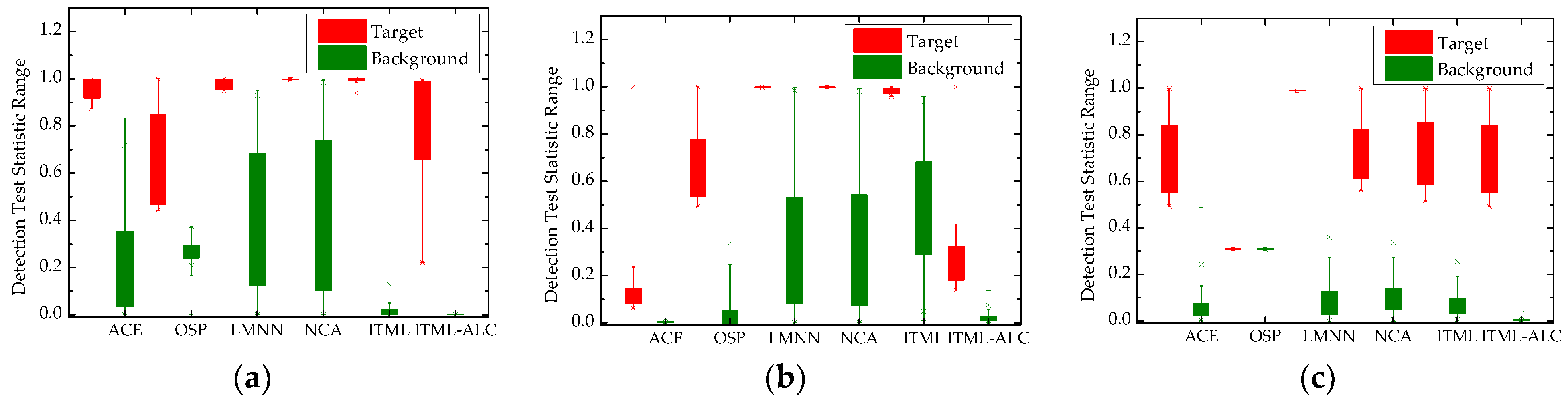
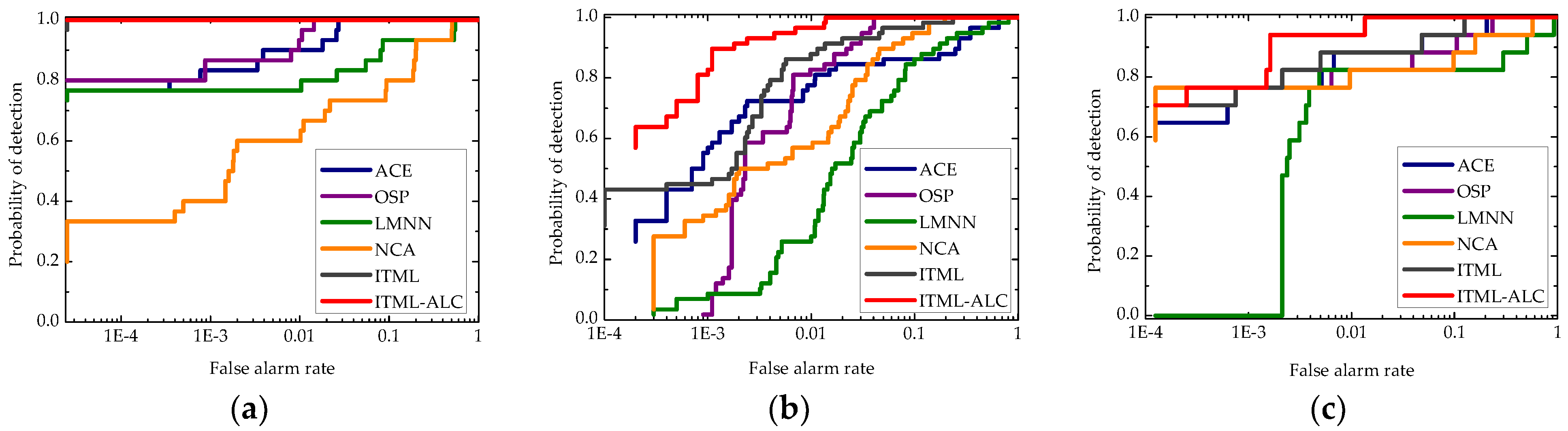
As metric learning-based methods, LMNN and NCA methods do not perform well (shown in Figure 7), and the cause may be that LMNN and NCA methods both have problems with handling high-dimensional data and are sensitive to the selection of initial points, leading to inability to achieve the optimal value if the parameters are not selected appropriately. To date, only a few researchers use distance metric learning for target detection. For example, reference [15] adopts LMNN and NCA as the comparison algorithms to prove the effectiveness of proposed supervised metric learning (SML) algorithm for the AVIRIS LCVF dataset. Though the implanted target locations of reference [15] are a little different compared to this paper, LMNN and NCA have poor similarity performance in both papers. When the value of FAR is equal to 10 × 10−4, the detection probabilities of LMNN in reference [15] and this paper are both about 80%. Similarly, in the two articles, the detection probability of NCA reaches 100% when the FAR is about 1, respectively. Moreover, although SML algorithm can recognize target pixels easily, the background pixels cannot be suppressed to an even lower value, compared with the ITML-ALC algorithm. This could be because that SML only use a similarity propagation constraint to simultaneously link target pixels and background ones, while ITML-ALC adopts adaptively local constraints to separate similar and dissimilar point-pairs.
(2)
For the HYDICE urban dataset, the FAR is reduced to a 10 2 level when the detection probability of ACE is at 80% in this paper, while FAR is reduced to a 10 2 level when the detection probability of ACE is at 70% in the reference [45]. Though they use different prior information, the ACE results of the different articles achieve a slightly different performance. Niu et al. [45] propose an adaptive weighted learning method (AWLM) using a self-completed background dictionary (SCBD) to extract the accurate target spectrum for hyperspectral target detection. When the FAR is reduced to 10 × 10−3, the detection probability of the proposed algorithm in reference [45] (named AWLM_SCBD+ACE) is at nearly 90%, while the detection probability of ITML-ALC in this paper is also at 90%. However, ITML-ALC only has trade-off parameter to be adjusted, but AWLM_SCBD+ACE additional parameters, i.e., κ and τ of adaptive weights, which can be used to suppress the influence of irrelevant pixels.
(3)
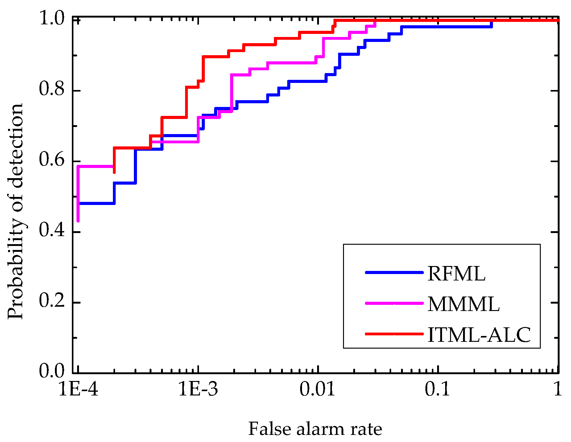
In addition, we compare ITML-ALC with MMML and RFML, which are previously proposed in [27] and [28], respectively. Figure 11 shows the corresponding ROC curves for the AVIRIS San Diego airport dataset. It can be found that ITML-ALC has similar performance when the FAR is less than 10 × 10−3, and then ITML-ALC outperforms other methods. Maybe because ITML-ALC can shrink the distances between samples of similar pairs and expand the distances between samples of dissimilar pairs compared with MMML and RFML.

5. Conclusions

In this paper, the adaptive information-theoretic metric learning with local constraints (ITML-ALC) algorithm has been proposed. Based on limited numbers of prior samples, the ITML-ALC algorithm constructs an efficient metric learning-based method without certain assumptions. Adaptively local constraints are then introduced to indicate the discriminative information for separating similar and dissimilar point-pairs with fewer parameters to be adjusted. By combining the ITML framework and adaptively local constraints, decision can be made by considering both the threshold and the changes between the distances before and after metric learning.
Extensive experiments, which are carried on three hyperspectral datasets for target detection, confirm the superior performance of the proposed ITML-ALC algorithm, which can obviously separate target samples from background ones. In general, the ITML-ALC algorithm presents a better detection performance and separability than the other classical target detectors.

Author Contributions

Y.D. and B.D. conceived, designed and performed the experiments; L.Z. and X.H. provided advice for the preparation and revision of the paper.

Funding

This work was supported in part by the Fundamental Research Funds for the Central Universities, China University of Geosciences (Wuhan) CUG170687; in part by the National Natural Science Foundation of China under Grant 61801444 and Grant 61471274.

Acknowledgments

The authors would like to thank the handling editor and anonymous reviewers for their careful reading and helpful remarks.

Conflicts of Interest

The authors declare no conflicts of interest.

References

  1. Manolakis, D.; Shaw, G. Detection Algorithms for Hyperspectral Imaging Applications. IEEE Signal Process. Mag. 2002, 19, 29–43. [Google Scholar] [CrossRef]
  2. Manolakis, D.; Truslow, E.; Pieper, M.; Cooley, T.; Brueggeman, M. Detection Algorithms in Hyperspectral Imaging Systems: An Overview of Practical Algorithms. IEEE Signal Process Mag. 2014, 31, 24–33. [Google Scholar] [CrossRef]
  3. Stefanou, M.S.; Kerekes, J.P. Image-Derived Prediction of Spectral Image Utility for Target Detection Applications. IEEE Trans. Geosci. Remote Sens. 2010, 48, 1827–1833. [Google Scholar] [CrossRef] [Green Version]
  4. Luo, H.; Liu, C.; Wu, C.; Guo, X. Urban Change Detection Based on Dempster–Shafer Theory for Multitemporal Very High–Resolution Imagery. Remote Sens. 2018, 10, 980. [Google Scholar] [CrossRef]
  5. Zou, Z.; Shi, Z. Random Access Memories: A New Paradigm for Target Detection in High Resolution Aerial Remote Sensing Images. IEEE Trans. Geosci. Remote Sens. 2018, 27, 1100–1111. [Google Scholar] [CrossRef] [PubMed]
  6. Manolakis, D.; Marden, D.; Shaw, G.A. Hyperspectral Image Processing for Automatic Target Detection Applications. J. Lincoln Lab. 2003, 14, 79–116. [Google Scholar]
  7. Lei, J.; Li, Y.; Zhao, D.; Xie, J.; Chang, C.I.; Wu, L.; Li, X.; Zhang, J.; Li, W. A Deep Pipelined Implementation of Hyperspectral Target Detection Algorithm on FPGA using HLS. Remote Sens. 2018, 10, 516. [Google Scholar] [CrossRef]
  8. Harsanyi, J.C.; Chang, C.I. Hyperspectral Image Classification and Dimensionality Reduction: An Orthogonal Subspace Projection Approach. IEEE Trans. Geosci. Remote Sens. 1994, 32, 779–785. [Google Scholar] [CrossRef]
  9. Kraut, S.; Scharf, L.L.; McWhorter, L.T. Adaptive Subspace Detectors. IEEE Trans. Signal Process. 2001, 49, 1–16. [Google Scholar] [CrossRef]
  10. Yang, C.; Tan, Y.; Bruzzone, L.; Lu, L.; Guan, R. Discriminative Feature Metric Learning in the Affinity Propagation Model for Band Selection in Hyperspectral Images. Remote Sens. 2017, 9, 782. [Google Scholar] [CrossRef]
  11. Zhang, L.; Zhang, Q.; Du, B.; Huang, X.; Tang, Y.Y.; Tao, D. Simultaneous Spectral–Spatial Feature Selection and Extraction for Hyperspectral Images. IEEE Trans. Cybern. 2018, 48, 16–28. [Google Scholar] [CrossRef] [PubMed]
  12. Kwon, H.; Nasrabadi, N.M. Kernel Matched Subspace Detectors for Hyperspectral Target Detection. IEEE Trans. Pattern Anal. Mach. Intell. 2006, 28, 178–194. [Google Scholar] [CrossRef] [PubMed]
  13. Kwon, H.; Nasrabadi, N.M. Kernel Spectral Matched Filter for Hyperspectral Imagery. Int. J. Comput. Vis. 2007, 71, 127–141. [Google Scholar] [CrossRef]
  14. Capobianco, L.; Garzelli, A.; Camps-Valls, G. Target Detection with Semisupervised Kernel Orthogonal Subspace Projection. IEEE Trans. Geosci. Remote Sens. 2009, 47, 3822–3833. [Google Scholar] [CrossRef]
  15. Zhang, L.; Zhang, L.; Tao, D.; Huang, X.; Du, B. Hyperspectral Remote Sensing Image Subpixel Target Detection Based on Supervised Metric Learning. IEEE Trans. Geosci. Remote Sens. 2014, 52, 4955–4965. [Google Scholar] [CrossRef]
  16. Gu, Y.; Chanussot, J.; Jia, X.; Benediktsson, J.A. Multiple Kernel Learning for Hyperspectral Image Classification: A Review. IEEE Trans. Geosci. Remote Sens. 2017, 55, 6547–6565. [Google Scholar] [CrossRef]
  17. Yuan, Y.; Zheng, X.; Lu, X. Spectral–spatial Kernel Regularized for Hyperspectral Image Denoising. IEEE Trans. Geosci. Remote Sens. 2015, 53, 3815–3832. [Google Scholar] [CrossRef]
  18. Gu, Y.; Liu, T.; Jia, X.; Benediktsson, J.A.; Chanussot, J. Nonlinear Multiple Kernel Learning with Multi–Structure–Element Extended Morphological Profiles for Hyperspectral Image Classification. IEEE Trans. Geosci. Remote Sens. 2016, 54, 3235–3247. [Google Scholar] [CrossRef]
  19. Luo, F.; Du, B.; Zhang, L.; Zhang, L.; Tao, D. Feature Learning Using Spatial–Spectral Hypergraph Discriminant Analysis for Hyperspectral Image. IEEE Trans. Cybern. 2018. [Google Scholar] [CrossRef] [PubMed]
  20. Dong, Y.; Du, B.; Zhang, L.; Zhang, L. Exploring Locally Adaptive Dimensionality Reduction for Hyperspectral Image Classification: A Maximum Margin Metric Learning Aspect. IEEE J. Sel. Top. Appl. Earth Obs. Remote Sens. 2017, 10, 1136–1150. [Google Scholar] [CrossRef]
  21. Zhang, L.; Zhang, L.; Tao, D.; Huang, X. Sparse Transfer Manifold Embedding for Hyperspectral Target Detection. IEEE Trans. Geosci. Remote Sens. 2014, 52, 1030–1043. [Google Scholar] [CrossRef]
  22. Zhang, Y.; Du, B.; Zhang, L.; Liu, T. Joint Sparse Representation and Multitask Learning for Hyperspectral Target Detection. IEEE Trans. Geosci. Remote Sens. 2017, 55, 894–906. [Google Scholar] [CrossRef]
  23. Lu, X.; Zhang, W.; Li, X. A Hybrid Sparsity and Distance–based Discrimination Detector for Hyperspectral Images. IEEE Trans. Geosci. Remote Sens. 2018, 56, 1704–1717. [Google Scholar] [CrossRef]
  24. Dong, Y.; Du, B.; Zhang, L.; Zhang, L. Dimensionality Reduction and Classification of Hyperspectral Images Using Ensemble Discriminative Local Metric Learning. IEEE Trans. Geosci. Remote Sens. 2017, 55, 2509–2524. [Google Scholar] [CrossRef]
  25. Du, B.; Zhang, L. A Discriminative Metric Learning Based Anomaly Detection Method. IEEE Trans. Geosci. Remote Sens. 2014, 52, 6844–6857. [Google Scholar]
  26. Gu, Y.; Feng, K. Optimized Laplacian Svm with Distance Metric Learning for Hyperspectral Image Classification. IEEE J. Sel. Top. Appl. Earth Obs. Remote Sens. 2013, 6, 1109–1117. [Google Scholar] [CrossRef]
  27. Dong, Y.; Zhang, L.; Zhang, L.; Du, B. Maximum Margin Metric Learning Based Target Detection for Hyperspectral Images. ISPRS J. Photogramm. Remote Sens. 2015, 108, 138–150. [Google Scholar] [CrossRef]
  28. Dong, Y.; Du, B.; Zhang, L. Target Detection Based on Random Forest Metric Learning. IEEE J. Sel. Top. Appl. Earth Obs. Remote Sens. 2015, 8, 1830–1838. [Google Scholar] [CrossRef]
  29. Goldberger, J.; Roweis, S.; Hinton, G.; Salakhutdinov, R. Neighbourhood Components Analysis. In Proceedings of the 17th International Conference on Neural Information Processing Systems (NIPS), Vancouver, BC, Canada, 13–18 December 2004; pp. 513–520. [Google Scholar]
  30. Weinberger, K.Q.; Saul, L.K. Distance Metric Learning for Large Margin Nearest Neighbor Classification. J. Mach. Learn. Res. 2009, 10, 207–244. [Google Scholar]
  31. Davis, J.V.; Kulis, B.; Jain, P.; Sra, S.; Dhillon, I.S. Information—Theoretic Metric Learning. In Proceedings of the 24th International Conference on Machine Learning (ICML), New York, NY, USA, 20–24 June 2007; pp. 209–216. [Google Scholar]
  32. Yang, X.; Wang, M.; Tao, D. Person Re–Identification with Metric Learning using Privileged Information. IEEE Trans. Image Process. 2018, 27, 791–805. [Google Scholar] [CrossRef] [PubMed]
  33. Wang, Q.; Zuo, W.; Zhang, L.; Li, P. Shrinkage Expansion Adaptive Metric Learning. In Proceedings of the 13th European Conference on Computer Vision (ECCV), Zurich, Switzerland, 6–12 September 2014; pp. 456–471. [Google Scholar]
  34. Luo, Y.; Wen, Y.; Liu, T.; Tao, D. Transferring Knowledge Fragments for Learning Distance Metric from a Heterogeneous Domain. IEEE Trans. Pattern Anal. Mach. Intell. 2018. [Google Scholar] [CrossRef] [PubMed]
  35. Han, J.; Zhang, D.; Cheng, G.; Guo, L.; Ren, J. Object Detection in Optical Remote Sensing Images Based on Weakly Supervised Learning and High-Level Feature Learning. IEEE Trans. Geosci. Remote Sens. 2015, 53, 3325–3337. [Google Scholar] [CrossRef] [Green Version]
  36. Zheng, X.; Yuan, Y.; Lu, X. Dimensionality Reduction by Spatial–spectral Preservation in Selected Bands. IEEE Trans. Image Process. 2017, 55, 5185–5197. [Google Scholar] [CrossRef]
  37. Li, Z.; Chang, S.; Liang, F.; Huang, T.S.; Cao, L.; Smith, J.R. Learning Locally—Adaptive Decision Functions for Person Verification. In Proceedings of the IEEE Computer Vision and Pattern Recognition (CVPR), Washington, DC, USA, 23–28 June 2013; pp. 3610–3617. [Google Scholar]
  38. Su, H.; Zhao, B.; Du, Q.; Du, P.; Xue, Z. Multifeature Dictionary Learning for Collaborative Representation Classification of Hyperspectral Imagery. IEEE Trans. Geosci. Remote Sens. 2018, 99, 1–18. [Google Scholar] [CrossRef]
  39. Chang, C.I.; Du, Q. Estimation of Number of Spectrally Distinct Signal Sources in Hyperspectral Imagery. IEEE Trans. Geosci. Remote Sens. 2004, 42, 608–619. [Google Scholar] [CrossRef] [Green Version]
  40. Du, B.; Zhang, L. Target Detection Based on a Dynamic Subspace. Pattern Recogn. 2014, 47, 344–358. [Google Scholar] [CrossRef]
  41. Messinger, D.; Ziemann, A.; Schlamm, A.; Basener, B. Spectral Image Complexity Estimated through Local Convex Hull Volume. Available online: https://ieeexplore.ieee.org/abstract/document/5594869/ (accessed on 3 September 2018).
  42. Ma, L.; Crawford, M.; Tian, J. Anomaly Detection for Hyperspectral Images Based on Robust Locally Linear Embedding. J. Infrared Millim. Terahertz 2010, 31, 753–762. [Google Scholar] [CrossRef]
  43. Lobo, J.M.; Jiménez-Valverde, A.; Real, R. AUC: A Misleading Measure of the Performance of Predictive Distribution Models. Global Ecol. Biogeogr. 2008, 17, 145–151. [Google Scholar] [CrossRef]
  44. Bioucas-Dias, J.; Plaza, A.; Camps-Valls, G.; Scheunders, P.; Nasrabadi, N.; Chanussot, J. Hyperspectral Remote Sensing Data Analysis and Future Challenges. IEEE Geosci. Remote Sens. Mag. 2013, 1, 6–36. [Google Scholar] [CrossRef] [Green Version]
  45. Niu, Y.; Wang, B. Extracting Target Spectrum for Hyperspectral Target Detection: An Adaptive Weighted Learning Method Using a Self-Completed Background Dictionary. IEEE Trans. Geosci. Remote Sens. 2017, 55, 1604–1617. [Google Scholar] [CrossRef]
Figure 1. Schematic illustration of adaptive information-theoretic metric learning with local constraints (ITML-ALC) algorithm for HSI target detection.
Remotesensing 10 01415 g001
Figure 2. AVIRIS LCVF dataset for the experiment. (a) Image scene; (b) Implanted target locations in the image; (c) Implanted pure target spectrum and some representative background samples spectra; (d) Locations of the background samples given in (c).
Remotesensing 10 01415 g002
Figure 3. AVIRIS San Diego airport dataset for the experiment. (a) Image scene; (b) The true locations of the targets; (c) Spectra of mean target pixels and some representative background samples.
Remotesensing 10 01415 g003
Figure 4. HYDICE urban dataset for the experiment. (a) Image scene; (b) The true locations of the targets; (c) Spectra of mean target pixels and some representative background samples.
Remotesensing 10 01415 g004
Figure 5. The AUCs of the proposed ITML-ALC method with respect to parameter γ . (a) AVIRIS LCVF dataset; (b) AVIRIS San Diego airport dataset; (c) HYDICE urban dataset.
Remotesensing 10 01415 g005
Figure 6. Detection maps and target detection test statistic plots of the AVIRIS LCVF dataset. (a) ACE; (b) OSP; (c) LMNN; (d) NCA; (e) ITML; (f) ITML-ALC.
Remotesensing 10 01415 g006
Figure 7. ROC curves of the different algorithms. (a) AVIRIS LCVF dataset; (b) AVIRIS San Diego airport dataset; (c) HYDICE urban dataset.
Remotesensing 10 01415 g007
Figure 8. The AUCs of the different algorithms. (a) AVIRIS LCVF dataset; (b) AVIRIS San Diego airport dataset; (c) HYDICE urban dataset.
Remotesensing 10 01415 g008
Figure 9. The FARs under 100% detection of the different algorithms. (a) AVIRIS LCVF dataset; (b) AVIRIS San Diego airport dataset; (c) HYDICE urban dataset.
Remotesensing 10 01415 g009
Figure 10. Target-background separation maps of the different algorithms. (a) AVIRIS LCVF dataset; (b) AVIRIS San Diego airport dataset; (c) HYDICE urban dataset.
Remotesensing 10 01415 g010
Figure 11. ROC curves of the different algorithms for AVIRIS San Diego airport dataset.
Remotesensing 10 01415 g011
Table 1. Details of the implanted target panels for the AVIRIS LCVF dataset.
Color of Target PanelSample IndexLine IndexFraction
Remotesensing 10 01415 i00150(75, 76) (100, 101) (125, 126)10%
Remotesensing 10 01415 i00275(75, 76) (100, 101) (125, 126)20%
Remotesensing 10 01415 i003100(75, 76) (100, 101) (125, 126)30%
Remotesensing 10 01415 i004125(75, 76) (100, 101) (125, 126)40%
Remotesensing 10 01415 i005150(75, 76) (100, 101) (125, 126)50%
Table 2. Details of the experimental images acquired from different sensors.
Experimental DatasetLCVF DatasetSan Diego Airport DatasetUrban Dataset
SensorAVIRISACIRISHYDICE
Spectral band224224210
Spatial resolution20 m3.5 m3 m
Wavelength370–2510 nm370–2510 nm400–2500 nm
Image size 200 × 200 100 × 100 80 × 100

