Statistical Machine Learning Methods and Remote Sensing for Sustainable Development Goals: A Review


Abstract
:
1. Introduction
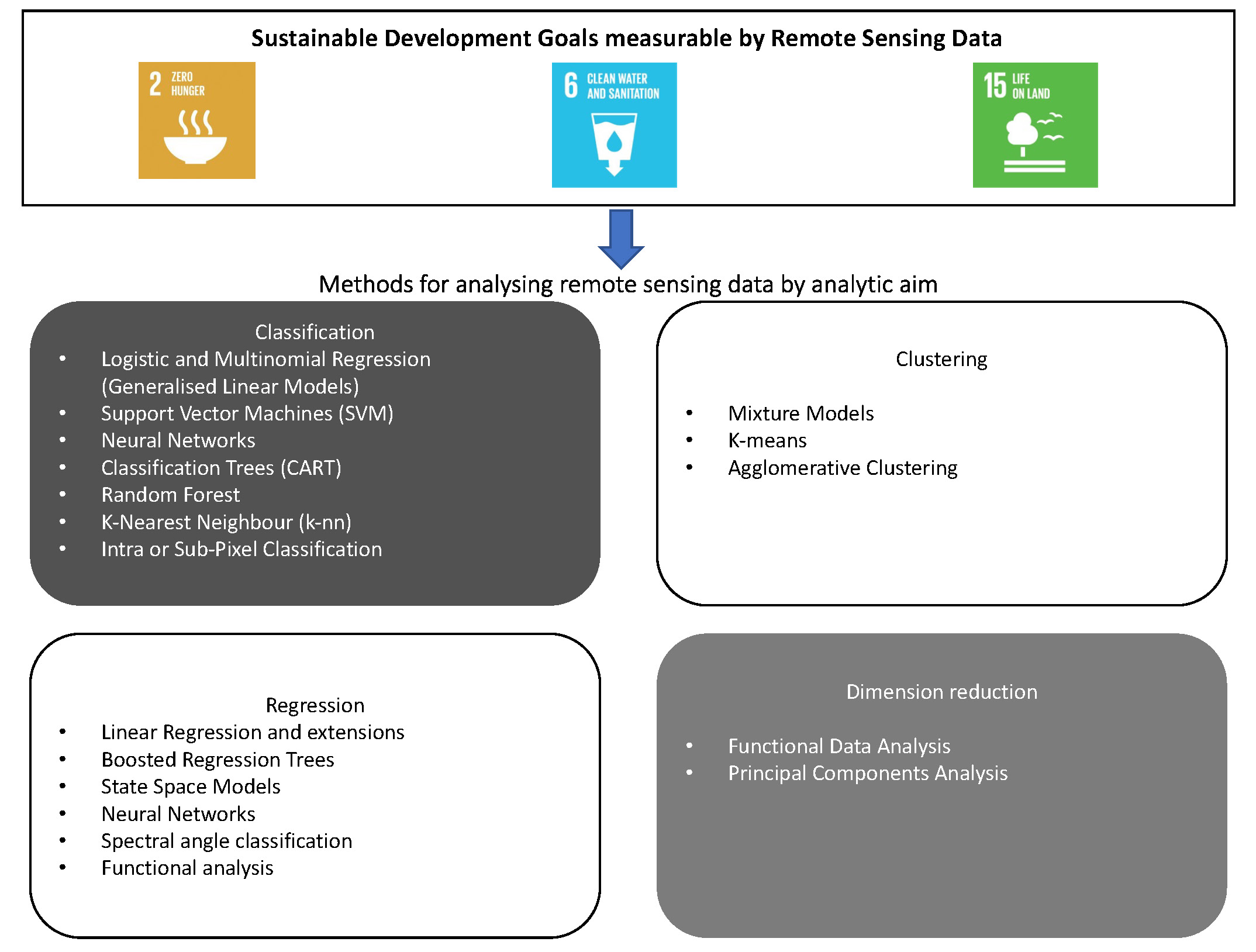
2. Remote Sensing for Environmental and Agricultural Statistics and SDG Indicators
3. Conducting SML Analyses
4. Analysis Step
- Of what phenomena is knowledge required, and what measures are required to provide this knowledge?
- what statistics will be used to estimate these measures? and
- what data are required to obtain these statistics?
4.1. Statistical Machine Learning Methods
4.2. Informed Statistical Machine Learning Methods
4.3. Physics Based Methods
4.4. Object Based Image Analysis
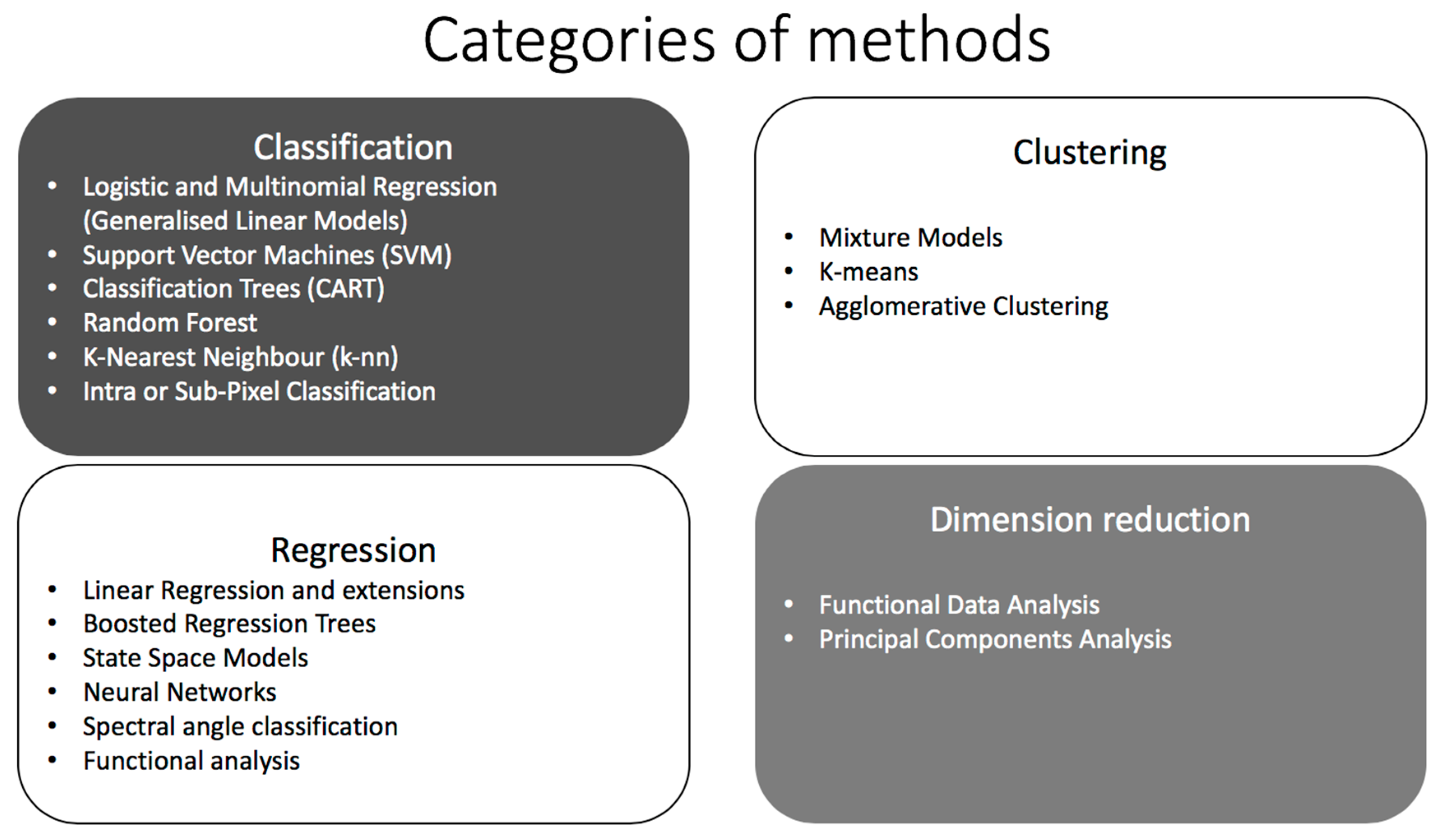
5. Categories of Statistical Machine Learning Methods
5.1. Classification
5.2. Clustering
5.3. Regression
5.4. Dimension Reduction
6. Statistical Machine Learning Methods for Time Series Data
- how do scientific methods relate to one another?
- is there any structure in my time-series dataset? and
- which methods will be helpful to classify time series in a particular dataset?
6.1. Classification
6.2. Clustering
- 1.
- Work directly on time series data either in frequency or time domain.The most common similarity measures used for direct comparison of time series include correlation, distance between data points, and information measures. Hierarchical clustering and k-means methods are then applied to these measures.
- 2.
- Work indirectly with features extracted from time series.The most common features extracted from time series data include points identified visually, via transformations of the data, or via dimension reduction. The most common distance measure is the Euclidean distance, although Kullback-Liebler and geometric distances are also used.
- 3.
- Work with models built from the time series.The most common time series models include moving average (MA), autoregressive (AR) and autoregressive moving average (ARMA) models and variants, State Space Models (SSM) which are a form of hidden Markov models (HMM), and fuzzy set methods.
6.3. Regression
6.4. Dimension Reduction
7. Ensemble Approaches
8. Overview of Methods
9. Conclusions
Supplementary Materials
Author Contributions
Funding
Acknowledgments
Conflicts of Interest
References
- Landgrebe, D. Early History of LARS. Available online: https://www.lars.purdue.edu/home/LARSHistory.html (accessed on 2 August 2018).
- Anderson, K.; Ryan, B.; Sonntag, W.; Kavvada, A.; Friedl, L. Earth observation in service of the 2030 Agenda for Sustainable Development. Geo-Spat. Inf. Sci. 2017, 20, 77–96. [Google Scholar] [CrossRef]
- European Space Agency Earth Observation for Sustainable Development. Available online: http://eo4sd.esa.int/ (accessed on 10 April 2018).
- United Nations United Nations Global Working Group on Big Data for Official Statistics. Available online: https://unstats.un.org/bigdata/ (accessed on 10 April 2018).
- Statistics Canada Integrated Crop Yield Modelling Using Remote Sensing, Agroclimatic Data and Survey Data. Available online: http://www23.statcan.gc.ca/imdb-bmdi/document/5225_D1_T9_V1-eng.htm (accessed on 10 April 2018 ).
- Imran, M.; Stein, A.; Zurita-Milla, R. Investigating rural poverty and marginality in Burkina Faso using remote sensing-based products. Int. J. Appl. Earth Obs. Geoinf. 2014, 26, 322–334. [Google Scholar] [CrossRef]
- Xie, M.; Jean, N.; Burke, M.; Lobell, D.; Ermon, S. Transfer Learning from Deep Features for Remote Sensing and Poverty Mapping. Available online: https://arxiv.org/abs/1510.00098 (accessed on 10 April 2018).
- United Nations SEEA Experimental Ecosystem Accounting. Available online: https://unstats.un.org/unsd/envaccounting/eea_project/default.asp (accessed on 10 April 2018).
- Committee on Earth Observation Satellites. Ceos eo Handbook Special 2018 Edition. Available online: http://eohandbook.com/sdg/index.html (accessed on 10 April 2018).
- Earth Observations for Official Statistics: Satellite Imagery and Geospatial Data Task Team Report. 2017. Available online: https://unstats.un.org/bigdata/taskteams/satellite/UNGWG_Satellite_Task_Team_Report_WhiteCover.pdf (accessed on 10 April 2018).
- García, L.; Rodríguez, J.D.; Wijnen, M.; Pakulski, I. Earth Observation for Water Resources. In Management: Current Use and Future Opportunities for the Water Sector; García, L., Rodríguez, D., Wijnen, M., Pakulski, I., Eds.; The World Bank: Washington, DC, USA, 2016; Available online: http://elibrary.worldbank.org/doi/book/10.1596/978-1-4648-0475-5 (accessed on 10 April 2018).
- Liu, L.; Tang, H.; Caccetta, P.; Lehmann, E.A.; Hu, Y.; Wu, X. Mapping afforestation and deforestation from 1974 to 2012 using Landsat time-series stacks in Yulin District, a key region of the Three-North Shelter region, China. Environ. Monit. Assess. 2013, 185, 9949–9965. [Google Scholar] [CrossRef] [PubMed]
- Echeverria, C.; Coomes, D.; Salas, J.; Rey-Benayas, J.M.; Lara, A.; Newton, A. Rapid deforestation and fragmentation of Chilean Temperate Forests. Biol. Conserv. 2006, 130, 481–494. [Google Scholar] [CrossRef]
- Hansen, M.C.; Potapov, P.V.; Moore, R.; Hancher, M.; Turubanova, S.A.; Tyukavina, A.; Thau, D.; Stehman, S.V.; Goetz, S.J.; Loveland, T.R.; et al. High-resolution global maps of 21st-century forest cover change. Science 2013, 342, 850–853. [Google Scholar] [CrossRef] [PubMed]
- Yeom, J.-M.; Kim, H.-O. Comparison of NDVIs from GOCI and MODIS Data towards Improved Assessment of Crop Temporal Dynamics in the Case of Paddy Rice. Remote Sens. 2015, 7, 11326–11343. [Google Scholar] [CrossRef] [Green Version]
- FAO. Handbook on Remote Sensing for Agricultural Statistics. 2016. Available online: http://gsars.org/wp-content/uploads/2017/09/GS-REMOTE-SENSING-HANDBOOK-FINAL-04.pdf (accessed on 10 April 2018).
- Nations, U. Sustainable Development Goals: Sustainable Development Knowledge Platform. Available online: https://sustainabledevelopment.un.org/?menu=1300 (accessed on 29 June 2018).
- Wikle, C.K. A Kernel-Based Spectral Model for Non-Gaussian Spatio-Temporal Processes. Available online: http://journals.sagepub.com/doi/abs/10.1191/1471082x02st036oa?journalCode=smja (accessed on 19 April 2018).
- Dekker, A.G.; Peters, S.; Vos, R.; Rijkeboer, M. Remote sensing for inland water quality detection and monitoring: State-of-the-art application in Friesland waters. In GIS and Remote Sensing Techniques in Land- and Water-Management; Springer: Dordrecht, The Netherland, 2001; pp. 17–38. [Google Scholar]
- Phinn, S.R.; Dekker, A.G.; Brando, V.E.; Roelfsema, C.M. Mapping water quality and substrate cover in optically complex coastal and reef waters: An integrated approach. Mar. Pollut. Bull. 2005, 51, 459–469. [Google Scholar] [CrossRef] [PubMed]
- Tripathy, R.; Chaudhary, K.N.; Nigam, R.; Manjunath, K.R.; Chauhan, P.; Ray, S.S.; Parihar, J.S. Operational semi-physical spectral-spatial wheat yield model development. ISPRS Int. Arch. Photogramm. Remote Sens. Spat. Inf. Sci. 2014, XL-8, 977–982. [Google Scholar] [CrossRef]
- Angerer, J.P.; Stuth, J.W.; Wandera, F.P.; Kaitho, R.J. Use of Satellite-Derived Data to Improve Biophysical Model Output: An Example from Southern Kenya. 2005. Available online: https://vtechworks.lib.vt.edu/handle/10919/65682 (accessed on 13 April 2018).
- Watts, J.D.; Kimball, J.S.; Parmentier, F.J.W.; Sachs, T.; Rinne, J.; Zona, D.; Oechel, W.; Tagesson, T.; Jackowicz-Korcz nski, M.; Aurela, M.; et al. A satellite data driven biophysical modeling approach for estimating northern peatland and tundra CO2 and CH4 fluxes. Biogeosciences 1961, 11. [Google Scholar] [CrossRef]
- Gow, L. A Land Surface Temperature Model-Data Differencing Approach to Quantifying Subsurface Water Use by Vegetation: Application in the Condamine Region, South-Eastern Queensland; University of Queensland: Brisbane, Australia, 2016; Available online: https://espace.library.uq.edu.au/view/UQ:603403 (accessed on 16 April 2018).
- Wettle, M.; Hartmann, K.; Heege, T.; Mittal, A.S. Satellite Derived Bathymetry Using Physics-Based Algorithms and Multispectral Satellite Imagery. Available online: http://a-a-r-s.org/acrs/index.php/acrs/acrs-overview/proceedings-1?view=publication&task=show&id=1369 (accessed on 16 April 2018).
- Blaschke, T. Object based image analysis for remote sensing. ISPRS J. Photogramm. Remote Sens. 2010, 65, 2–16. [Google Scholar] [CrossRef]
- Hoque, M.A.-A.; Phinn, S.; Roelfsema, C.; Childs, I. Assessing tropical cyclone impacts using object-based moderate spatial resolution image analysis: A case study in Bangladesh. Int. J. Remote Sens. 2016, 37, 5320–5343. [Google Scholar] [CrossRef]
- Hoque, M.A.-A.; Phinn, S.; Roelfsema, C.; Childs, I. Modelling tropical cyclone risks for present and future climate change scenarios using geospatial techniques. Int. J. Digit. Earth 2018, 11, 246–263. [Google Scholar] [CrossRef]
- Tsai, Y.H.; Stow, D.; Weeks, J. Comparison of Object-Based Image Analysis Approaches to Mapping New Buildings in Accra, Ghana Using Multi-Temporal QuickBird Satellite Imagery. Remote Sens. 2011, 3, 2707–2726. [Google Scholar] [CrossRef] [Green Version]
- Blaschke, T.; Hay, G.J.; Kelly, M.; Lang, S.; Hofmann, P.; Addink, E.; Queiroz Feitosa, R.; van der Meer, F.; van der Werff, H.; van Coillie, F.; et al. Geographic Object-Based Image Analysis—Towards a new paradigm. ISPRS J. Photogramm. Remote Sens. 2014, 87, 180–191. [Google Scholar] [CrossRef] [PubMed]
- Hastie, T.; Tibshirani, R.; Friedman, J. The Elements of Statistical Learning, 2nd ed.; Springer: Berlin, Germany, 2008; ISBN 978-0-387-84857-0. [Google Scholar]
- Maggiori, E.; Tarabalka, Y.; Charpiat, G.; Alliez, P. Convolutional Neural Networks for Large-Scale Remote-Sensing Image Classification. IEEE Trans. Geosci. Remote Sens. 2017, 55, 645–657. [Google Scholar] [CrossRef]
- Song, H.; Liu, Q.; Wang, G.; Hang, R.; Huang, B. Spatiotemporal Satellite Image Fusion Using Deep Convolutional Neural Networks. IEEE J. Sel. Top. Appl. Earth Obs. Remote Sens. 2018, 11, 821–829. [Google Scholar] [CrossRef]
- Kavzoglu, T.; Mather, P.M. The use of backpropagating artificial neural networks in land cover classification. J. Int. J. Remote Sens. 2003, 2423, 143–1161. [Google Scholar] [CrossRef]
- Kavzoglu, T.; Reis, S. Performance Analysis of Maximum Likelihood and Artificial Neural Network Classifiers for Training Sets with Mixed Pixels. GISci. Remote Sens. 2008, 45, 330–342. [Google Scholar] [CrossRef]
- Shao, Y.; Lunetta, R.S. Comparison of support vector machine, neural network, and CART algorithms for the land-cover classification using limited training data points. ISPRS J. Photogramm. Remote Sens. 2012, 70, 78–87. [Google Scholar] [CrossRef]
- Wang, L.; Shi, C.; Diao, C.; Ji, W.; Yin, D. A survey of methods incorporating spatial information in image classification and spectral unmixing. Int. J. Remote Sens. 2016, 37, 3870–3910. [Google Scholar] [CrossRef] [Green Version]
- Wang, Q.; Shi, W.; Atkinson, P.M.; Li, Z. Land Cover Change Detection at Subpixel Resolution with a Hopfield Neural Network. IEEE J. Sel. Top. Appl. Earth Obs. Remote Sens. 2014, 8, 1–14. [Google Scholar] [CrossRef]
- Mayfield, H.; Smith, C.; Gallagher, M.; Hockings, M. Use of freely available datasets and machine learning methods in predicting deforestation. Environ. Model. Softw. 2017, 87, 17–28. [Google Scholar] [CrossRef]
- Zhu, X.X.; Tuia, D.; Mou, L.; Xia, G.-S.; Zhang, L.; Xu, F.; Fraundorfer, F. Deep Learning in Remote Sensing: A Comprehensive Review and List of Resources. IEEE Geosci. Remote Sens. Mag. 2017, 5, 8–36. [Google Scholar] [CrossRef] [Green Version]
- Espinoza-Molina, D.; Bahmanyar, R.; Datcu, M.; Diaz-Delgado, R.; Bustamante, J. Land-cover evolution class analysis in Image Time Series of Landsat and Sentinel-2 based on Latent Dirichlet Allocation. In Proceedings of the 2017 9th International Workshop on the Analysis of Multitemporal Remote Sensing Images (MultiTemp), Brugge, Belgium, 27–29 June 2017; pp. 1–4. [Google Scholar]
- Vance, C.; Geoghegan, J. Temporal and spatial modelling of tropical deforestation: A survival analysis linking satellite and household survey data. Agric. Econ. 2002, 27, 317–332. [Google Scholar] [CrossRef]
- Fulcher, B.D.; Little, M.A.; Jones, N.S. Highly comparative time-series analysis: The empirical structure of time series and their methods. J. R. Soc. Interface 2013, 10, 20130048. [Google Scholar] [CrossRef] [PubMed]
- Signals and Systems Group. A Compound Methodological Eye on Nature’s Signals. Available online: http://systems-signals.blogspot.com.au/2013/04/a-compound-methodological-eye-on.html (accessed on 16 April 2018).
- Nanopoulos, A.; Alcock, R.; Manolopoulos, Y. Feature-Based Classiication of Time-Series Data; Nova Science Publishers, Inc.: Commack, NY, USA, 2001; pp. 49–61. [Google Scholar]
- James, G.M. Curve Alignments by Moments. Ann. Appl. Stat. 2007, 1, 480–501. [Google Scholar] [CrossRef]
- Rani, S.; Sikka, G. Recent Techniques of Clustering of Time Series Data: A Survey. Int. J. Comput. Appl. 2012, 52, 975–8887. [Google Scholar] [CrossRef]
- Tahsin, S.; Medeiros, S.; Hooshyar, M.; Singh, A. Optical Cloud Pixel Recovery via Machine Learning. Remote Sens. 2017, 9, 527. [Google Scholar] [CrossRef]
- McCord, S.E.; Buenemann, M.; Karl, J.W.; Browning, D.M.; Hadley, B.C. Integrating Remotely Sensed Imagery and Existing Multiscale Field Data to Derive Rangeland Indicators: Application of Bayesian Additive Regression Trees. Rangel. Ecol. Manag. 2017, 70, 644–655. [Google Scholar] [CrossRef]
- Potgieter, A.B.; Apan, A.; Dunn, P.; Hammer, G. Estimating crop area using seasonal time series of Enhanced Vegetation Index from MODIS satellite imagery. Aust. J. Agric. Res. 2007, 58, 316. [Google Scholar] [CrossRef]
- Liu, C.; Ray, S.; Hooker, G.; Friedl, M. Functional Factor Analysis for Periodic Remote Sensing Data. Ann. Appl. Stat. 2012, 6, 601–624. [Google Scholar] [CrossRef]
- Du, P.; Xia, J.; Zhang, W.; Tan, K.; Liu, Y.; Liu, S. Multiple Classifier System for Remote Sensing Image Classification: A Review. Sensors 2012, 12, 4764–4792. [Google Scholar] [CrossRef] [PubMed] [Green Version]
- Woźniak, M.; Graña, M. A survey of multiple classifier systems as hybrid systems. Inf. Fusion 2014, 16, 3–17. [Google Scholar] [CrossRef]
- Ponti, M.P. Combining Classifiers: From the creation of ensembles to the decision fusion. In Proceedings of the 2011 24th SIBGRAPI Conference on Graphics, Patterns, and Images Tutorials, Alagoas, Brazil, 28–30 August 2011. [Google Scholar]
- Sweeney, S.; Ruseva, T.; Estes, L.; Evans, T. Mapping Cropland in Smallholder-Dominated Savannas: Integrating Remote Sensing Techniques and Probabilistic Modeling. Remote Sens 2015, 7, 15295–15317. [Google Scholar] [CrossRef] [Green Version]
- Neagoe, V.-E.; Chirila-Berbentea, V. A novel approach for semi-supervised classification of remote sensing images using a clustering-based selection of training data according to their GMM responsibilities. In Proceedings of the 2017 IEEE International Geoscience and Remote Sensing Symposium (IGARSS), Fort Worth, TX, USA, 23–28 July 2017; pp. 4730–4733. [Google Scholar]
- Huang, X.; Zhang, L. An SVM Ensemble Approach Combining Spectral, Structural, and Semantic Features for the Classification of High-Resolution Remotely Sensed Imagery. IEEE Trans. Geosci. Remote Sens. 2013, 51, 257–272. [Google Scholar] [CrossRef]
- Li, X.; Liu, X.; Yu, L. Aggregative model-based classifier ensemble for improving land-use/cover classification of Landsat TM Images. Int. J. Remote Sens. 2014, 35, 1481–1495. [Google Scholar] [CrossRef]
- Roy, M.; Ghosh, S.; Ghosh, A. A novel approach for change detection of remotely sensed images using semi-supervised multiple classifier system. Inf. Sci. 2014, 269, 35–47. [Google Scholar] [CrossRef]
- Bigdeli, B.; Samadzadegan, F.; Reinartz, P. Fusion of hyperspectral and LIDAR data using decision template-based fuzzy multiple classifier system. Int. J. Appl. Earth Obs. Geoinf. 2015, 38, 309–320. [Google Scholar] [CrossRef]
- Samat, A.; Du, P.; Baig, M.H.A.; Chakravarty, S.; Cheng, L. Ensemble Learning with Multiple Classifiers and Polarimetric Features for Polarized SAR Image Classification. Photogramm. Eng. Remote Sens. 2014, 80, 239–251. [Google Scholar] [CrossRef]
- Clinton, N.; Yu, L. Geographic stacking: Decision fusion to increase global land cover map accuracy. ISPRS J. Photogramm. Remote Sens. 2015, 103, 57–65. [Google Scholar] [CrossRef]
- Bavaghar, P.M. Deforestation modelling using logistic regression and GIS. J. For. Sci. 2015, 61, 193–199. [Google Scholar] [CrossRef]
- Hyandye, C.; Mandara, C.G.; Safari, J. GIS and Logit Regression Model Applications in Land Use/Land Cover Change and Distribution in Usangu Catchment. Am. J. Remote Sens. 2015, 3, 6–16. [Google Scholar] [CrossRef]
- Szuster, B.W.; Chen, Q.; Borger, M. A comparison of classification techniques to support land cover and land use analysis in tropical coastal zones. Appl. Geogr. 2011, 31, 525–532. [Google Scholar] [CrossRef]
- Mathur, A.; Foody, G.M. Crop classification by support vector machine with intelligently selected training data for an operational application. Int. J. Remote Sens. 2008, 29, 2227–2240. [Google Scholar] [CrossRef] [Green Version]
- Wu, K.-P.; Wang, S.-D. Choosing the kernel parameters for support vector machines by the inter-cluster distance in the feature space. Pattern Recognit. 2009, 42, 710–717. [Google Scholar] [CrossRef]
- Otukei, J.R.; Blaschke, T. Land cover change assessment using decision trees, support vector machines and maximum likelihood classification algorithms. Int. J. Appl. Earth Obs. Geoinf. 2010, 12, S27–S31. [Google Scholar] [CrossRef]
- Sharma, R.; Ghosh, A.; Joshi, P.K. Decision tree approach for classification of remotely sensed satellite data using open source support. J. Earth Syst. Sci. 2013, 122, 1237–1247. [Google Scholar] [CrossRef]
- Al-Obeidat, F.; Al-Taani, A.T.; Belacel, N.; Feltrin, L.; Banerjee, N. A Fuzzy Decision Tree for Processing Satellite Images and Landsat Data. Procedia Comput. Sci. 2015, 52, 1192–1197. [Google Scholar] [CrossRef]
- Chasmer, L.; Hopkinson, C.; Veness, T.; Quinton, W.; Baltzer, J. A decision-tree classification for low-lying complex land cover types within the zone of discontinuous permafrost. Remote Sens. Environ. 2014, 143, 73–84. [Google Scholar] [CrossRef]
- Dos Reis, A.A.; Carvalho, M.C.; de Mello, J.M.; Gomide, L.R.; Ferraz Filho, A.C.; Acerbi Junior, F.W. Spatial prediction of basal area and volume in Eucalyptus stands using Landsat TM data: An assessment of prediction methods. N. Z. J. For. Sci. 2018, 48, 1. [Google Scholar] [CrossRef]
- Schmidt, M.; Pringle, M.; Devadas, R.; Denham, R.; Tindall, D. A Framework for Large-Area Mapping of Past and Present Cropping Activity Using Seasonal Landsat Images and Time Series Metrics. Remote Sens. 2016, 8, 312. [Google Scholar] [CrossRef]
- McRoberts, R.E.; Tomppo, E.O.; Finley, A.O.; Heikkinen, J. Estimating areal means and variances of forest attributes using the k-Nearest Neighbors technique and satellite imagery. Remote Sens. Environ. 2007, 111, 466–480. [Google Scholar] [CrossRef]
- Ver Hoef, J.M.; Temesgen, H. A Comparison of the Spatial Linear Model to Nearest Neighbor (k-NN) Methods for Forestry Applications. PLoS ONE 2013, 8, e59129. [Google Scholar] [CrossRef] [PubMed]
- Blanzieri, E.; Melgani, F. Nearest Neighbor Classification of Remote Sensing Images With the Maximal Margin Principle. IEEE Trans. Geosci. Remote Sens. 2008, 46, 1804–1811. [Google Scholar] [CrossRef]
- Zhang, J.; Wei, F.; Sun, P.; Pan, Y.; Yuan, Z.; Yun, Y. A Stratified Temporal Spectral Mixture Analysis Model for Mapping Cropland Distribution through MODIS Time-Series Data. J. Agric. Sci. 2015, 7, 95. [Google Scholar] [CrossRef]
- Thenkabail, P.S. Remotely Sensed Data Characterization, Classification, and Accuracies; CRC Press: Boca Raton, FL, USA, 2015; ISBN 9781482217865. [Google Scholar]
- De Melo, A.C.O.; de Moraes, R.M.; dos Santos Machado, L. Gaussian Mixture Models for Supervised Classification of Remote Sensing Multispectral Images. In Lecture Notes in Computer Science; Springer: Berlin/Heidelberg, Germany, 2003; pp. 440–447. [Google Scholar]
- Walsh, S.J.; Shao, Y.; Mena, C.F.; McCleary, A.L. Integration of Hyperion Satellite Data and A Household Social Survey to Characterize the Causes and Consequences of Reforestation Patterns in the Northern Ecuadorian Amazon. Photogramm. Eng. Remote Sens. 2008, 74, 725–735. [Google Scholar] [CrossRef]
- Tao, J.; Shu, N.; Wang, Y.; Hu, Q.; Zhang, Y. A study of a Gaussian mixture model for urban land-cover mapping based on VHR remote sensing imagery. Int. J. Remote Sens. 2016, 37, 1–13. [Google Scholar] [CrossRef]
- Usman, B. Satellite Imagery Land Cover Classification using K-Means Clustering Algorithm Computer Vision for Environmental Information Extraction. Elixir Comput. Sci. Eng. 2013, 63, 18671–18675. [Google Scholar]
- Kamarudin, M.K.A.; Toriman, M.E.; Wahab, N.A.; Juahir, H.; Endut, A.; Umar, R.; Gasim, M.B. Development of stream classification system on tropical areas with statistical approval in Pahang River basin, Malaysia. Desalin. WATER Treat. 2017, 96, 237–254. [Google Scholar] [CrossRef]
- Liao, W.; Liu, X.; Wang, D.; Sheng, Y.; Yu, B.; Zhou, Y.; He, C.; Li, X.; Myint, S.; Thenkabail, P.S. The Impact of Energy Consumption on the Surface Urban Heat Island in China’s 32 Major Cities. Remote Sens. 2017, 9, 250. [Google Scholar] [CrossRef]
- Elith, J.; Leathwick, J.R.; Hastie, T. A working guide to boosted regression trees. J. Anim. Ecol. 2008, 77, 802–813. [Google Scholar] [CrossRef] [PubMed] [Green Version]
- Safari, A.; Sohrabi, H.; Powell, S.; Shataee, S. A comparative assessment of multi-temporal Landsat 8 and machine learning algorithms for estimating aboveground carbon stock in coppice oak forests. Int. J. Remote Sens. 2017, 38, 6407–6432. [Google Scholar] [CrossRef]
- Youssef, A.M.; Pourghasemi, H.R.; Pourtaghi, Z.S.; Al-Katheeri, M.M. Landslide susceptibility mapping using random forest, boosted regression tree, classification and regression tree, and general linear models and comparison of their performance at Wadi Tayyah Basin, Asir Region, Saudi Arabia. Landslides 2016, 13, 839–856. [Google Scholar] [CrossRef]
- Wendroth, O.; Reuter, H.I.; Kersebaum, K.C. Predicting yield of barley across a landscape: A state-space modeling approach. J. Hydrol. 2003, 272, 250–263. [Google Scholar] [CrossRef]
- Schneibel, A.; Frantz, D.; Röder, A.; Stellmes, M.; Fischer, K.; Hill, J. Using Annual Landsat Time Series for the Detection of Dry Forest Degradation Processes in South-Central Angola. Remote Sens. 2017, 9, 905. [Google Scholar] [CrossRef]
- Srivastava, P.K.; Han, D.; Rico-Ramirez, M.A.; Bray, M.; Islam, T. Selection of classification techniques for land use/land cover change investigation. Adv. Sp. Res. 2012, 50, 1250–1265. [Google Scholar] [CrossRef]
- Kong, Y.-L.; Huang, Q.; Wang, C.; Chen, J.; Chen, J.; He, D. Long Short-Term Memory Neural Networks for Online Disturbance Detection in Satellite Image Time Series. Remote Sens. 2018, 10, 452. [Google Scholar] [CrossRef]
- Reddy, D.S.; Prasad, P.R.C. Prediction of vegetation dynamics using NDVI time series data and LSTM. Model. Earth Syst. Environ. 2018, 4, 409–419. [Google Scholar] [CrossRef]
- Mia, B.; Fujimitsu, Y. Mapping hydrothermal altered mineral deposits using Landsat 7 ETM+ image in and around Kuju volcano, Kyushu, Japan. J. Earth Syst. Sci. 2012, 121, 1049–1057. [Google Scholar] [CrossRef]
- Escabias, M.; Aguilera, A.M.; Valderrama, M.J. Modeling environmental data by functional principal component logistic regression. Environmetrics 2005, 16, 95–107. [Google Scholar] [CrossRef]
- Hogland, J.; Billor, N.; Anderson, N. Comparison of standard maximum likelihood classification and polytomous logistic regression used in remote sensing. Eur. J. Remote Sens. 2013, 46, 623–640. [Google Scholar] [CrossRef]
- Yang, C.; Everitt, J.H.; Murden, D. Evaluating high resolution SPOT 5 satellite imagery for crop identification. Comput. Electron. Agric. 2011, 75, 347–354. [Google Scholar] [CrossRef]
- Melgani, F.; Bruzzone, L. Classification of hyperspectral remote sensing images with support vector machines. IEEE Trans. Geosci. Remote Sens. 2004, 42, 1778–1790. [Google Scholar] [CrossRef] [Green Version]


| Sustainable Development Goal | Sustainable Development Target Description | Remote Sensing Application and Indicator |
|---|---|---|
Goal 2: End Hunger  | End hunger, achieve food security and improved nutrition, and promote sustainable agriculture. By 2030, ensure sustainable food production systems and implement resilient agricultural practices that increase productivity and production, that help maintain ecosystems, that strengthen capacity for adaptation to climate change, extreme weather, drought, flooding, and other disasters, and that progressively improve land and soil quality. | Crop area estimation, crop yield, land cover classification, extreme weather event detection. Indicator 2.4.1 Proportion of agricultural area under productive and sustainable agriculture. |
Goal 6: Clean water and sanitation  | Ensure availability and sustainable management of water and sanitation for all. By 2020, protect and restore water-related ecosystems, including mountains, forests, wetlands, rivers, aquifers, and lakes. | Water quality monitoring. Indicator 6.6.1 Change in the extent of water-related ecosystems over time. Indicator 6.3.2 Proportion of bodies of water with good ambient water quality. |
Goal 15: Life on land  | Protect, restore, and promote sustainable use of terrestrial ecosystems, sustainably manage forests, combat desertification, halt and reverse land degradation, and halt biodiversity loss. By 2020, ensure the conservation, restoration, and sustainable use of terrestrial and inland freshwater ecosystems and their services, in particular forests, wetlands, mountains, and drylands, in line with obligations under international agreements. | Forest cover monitoring, deforestation detection. Indicator 15.1.1 Forest area as a proportion of total land area. Indicator 15.3.1 Proportion of land that is degraded over total land area. Indicator 15.4.2 Mountain Green Cover Index. |
| Method Description | Applications |
|---|---|
| Analytic Aim: Classification | |
| Logistic and Multinomial Regression Types of generalised linear models (glm). Logistic regression is used when the response variable is categorical with two levels (vegetation/not vegetation, high/low, present/absent). Multinomial logistic regression is used when the response variable has more than two levels (trees/grass/bare ground/crop/water, high/medium/low). | Bavaghar (2015) [63] used logistic regression on satellite imagery data to estimate the location and extent of deforestation based on variables, such as slope, distance to roads, and residential areas, and highlights in particular the ability to quantify the uncertainty in predictions as a strength of the approach. An overall 75% correct classification rate was obtained, with an estimate of 12% deforestation of the total study site over the 27 years from 1967 to 1994. Hyandye et al. (2015) [64] used multinomial logistic regression to determine how land use/land cover class in Usangu, Tanzania was influenced by a set of covariates; slope, elevation, distance from roads, distance from rivers, population density, annual rainfall, Normalized Difference Vegetation Index (NDVI), and soil types. The authors used the multinomial model, run on Landsat of data across multiple years, to obtain the probable change in land use/land cover given a one unit change in these covariates. |
| Support Vector Machines (SVM) SVMs are a class of non-parametric supervised classification techniques. In their simplest form, 2-class SVMs are linear binary classifiers. The term, “support vector”, refers to the points lying on the separation margin between the data groups or classes. SVMs can be used to map the support vectors in higher dimensional feature spaces to make them more separable, and then classified in the original input space. Kernel functions are used to define this mapping from the input space to the feature space. | Some papers that examine the use of SVMs for analysis of remote sensing data include Szuster (2011) [65] for land use and land cover classification in tropical coastal zones; Mathur and Foody (2008) [66] for crop classification; and Shao and Lunetta (2012) [36] for land classification. Wu and Wang (2009) [67] and Hastie, Tibshirani, and Friedman (2008) [31] provide helpful explanations of kernels and guidance on how to select an appropriate kernel for SVMs. |
| Classification and Regression Trees (CART) A supervised classification technique that represents class memberships as “leaves” and input variables are “nodes”. Branches are formed from these nodes based on splitting the values of the input variables to best group the data. A classification tree is a member of the family of decision tree methods, which include regression trees, boosted trees, bagged trees, and so on. The main advantage of classification trees in particular, and decision trees in general, is they are simple and easy to understand. Due to their computational simplicity they can be applied to large amounts of data. | Lawrence and Wright (2001) employed this method to classify land cover in the Yellowstone ecosystem in the USA, based on Landsat TM imagery. Otukei and Blaschke (2010) [68] used a maximum likelihood classifier, support vector machine, and decision trees to identify land cover change in satellite imagery. They found decision trees generally outperformed the other two methods and had an accuracy of over 85%. More recent references to decision trees and remote sensing include Sharma et al. (2013) [69], Al-Obeidat et al. (2015) [70], and Chasmer et al. (2014) [71]. |
| Random forest A type of classification tree method, which is a set of ‘shallow’ trees constructed from many random samples. The method combines the results of these trees to classify or predict values. | dos Reis et al. (2018) [72] applied a number of methods to mapping the basal area and volume of Eucalyptus forest in Brazil, and found random forest was the best method for this spatial prediction, compared with multiple linear regression, SVM, and artificial neural network methods. Schmidt et al. (2016) [73] compared a number of methods for classifying crop/no crop in Australia using Landsat imagery, and found that random forests provided the best accuracy and robustness. |
| K nearest neighbour (K-nn) A well-known and popular nonparametric classification technique due to their relative simplicity. In their simplest form, an observation is classified according to a majority vote of its k nearest neighbours. That is, an object’s class is assigned to it by the most common class among its k nearest neighbours, where k is generally a small positive integer. Although nearest neighbour methods are conceptually appealing and computationally fast, they are not always the best model for remote sensing data and are sometimes combined with other methods in this context. | McRoberts et al. (2007) [74] employed k-nn methodology for forest inventory mapping and estimation using Landsat imagery to derive 12 satellite image-based predictor variables, NDVI, and the Tassel Cap (TC) transformations (brightness, greenness, wetness). Ver Hoef and Temesgen (2013) [75] compared k-nn and spatial linear models for forestry applications and preferred the spatial model. However, their accuracy and predictive capability can be improved by combining them with other models. For example, Blanzieri and Melgani (2008) [76] preferred a combination of k-nn and SVM methods for classification of remote sensing images. |
| Intra or sub-pixel classification These methods can be used to address the issue of so-called “mixed” pixels; pixels that display characteristics of more than one group. Mixed pixels are mainly a concern in coarse (e.g., MODIS) or moderate (e.g., Landsat) resolution remotely sensed data. The two most common approaches in the remote sensing literature to the mixed pixel classification problem are spectral mixture analysis (SMA) and soft, or fuzzy, classifiers. | Zhang et al. (2015) [77] propose a stratified temporal spectral mixture analysis (STSMA) for cropland area estimation using MODIS time-series data. Discussion of advantages and disadvantages of SMA for analysis of remotely sensed data are given by Thenkabail [78]. |
| Analytic Aim: Clustering | |
| Mixture models Models based on the premise that observed data arise from various sources or groups. Each group is assumed to have a particular distribution. The mixture model is then a weighted sum of these distributions, where the weights correspond to the proportion of observations in the population that belong to that group; this can also be interpreted as the probability that an observation belongs to that particular group. These methods are also known as soft, or fuzzy, classifiers. | de Melo et al. (2003) [79] used mixture models for supervised classification of remote sensing multispectral images in an area of Tapajós River in Brazil, and Walsh (2008) [80], who combine secondary forest estimates derived from remote sensing data and a household survey to characterise causes and consequences of reforestation in an area in the Northern Ecuadorian Amazon. More recently, Tao et al. (2016) [81] employed a Gaussian mixture model to estimate and map urban land cover using remote sensing images with very high resolution. |
| K-means One of the most common clustering approaches used in machine learning. The algorithm assumes the data is drawn from K different clusters and assigns each unlabeled point to the closest group centre, which are recalculated until no changes occur. K-means can also be used for dimension reduction; a value of k is chosen, which is large, but much smaller than the original number of pixels, and the resultant clusters are then used for further classification, regression or other analysis. | Usman (2013) [82] used a k-means approach to classify high resolution satellite imagery data into classes, which were then determined to farmland, bare land, and built up areas. Yuan et al. (2015) used k-means to cluster land use in remotely sensed data that had already been pre-processed using functional analysis. |
| Agglomerative clustering A popular clustering method. The algorithm starts with each point as its own cluster and iteratively merges the closest clusters until a stopping rule is reached. | Kamarudin et al. (2017) [83] used hierarchical agglomerative cluster analysis on remote sensing, GIS, and a river hydrographic survey to develop a stream classification system for tropical areas in Peninsular Malaysia. |
| Analytic Aim: Regression | |
| Linear regression One of the most common empirical models. The response variable is used in its natural form or it is transformed to be more symmetric, for example, through a log transformation if the distribution is very skew. The response is then estimated by a linear combination of covariates. These covariates can take their original form or be transformed to describe non-linear relationships between the response variable and covariates e.g., polynomial transformation to describe nonlinear relationships with the response or combinations of covariates to describe interactions. | Liao (2017) [84] used linear regression to determine the impact of energy consumption on surface temperature in urban areas. The focus of the study was on 32 major cities in China and used the sum of nighttime lights in each province. Schmidt et al. (2016) [73] used linear regression to predict reflectance at t0 in synthetic spectral images based on archived satellite images. |
| Boosted Regression Trees A boosted regression tree is a combination of single decision trees. This provides the added benefit of boosting, which improves the predictive performance by combining simple tree models. Elith et al. (2008) [85] describe benefits of boosted regression trees, including the ability to fit complex nonlinear relationships and handle interaction effects between predictors. These models can also accommodate missing data and do not require data transformation or the removal of outliers. | Safari et al. (2017) [86] used boosted regression trees to estimate carbon stocks in forests based on Landsat 8 satellite images and field data. They found this method was outperformed by random forest and support vector machine algorithms in terms of R2 and root mean square error (RMSE), but produced less biased results than the support vector machine. Youssef et al. (2016) [87] applied boosted regression tree algorithms to satellite images to produce landslide susceptibility maps. |
| State Space Models A common form of spatio-temporal model that can provide a natural setting for analysing time series of remote sensing data, particularly if the process to be modelled can be viewed as one that is spatially evolving through time. | State space models have been employed for crop estimation and prediction for over 15 years. For example, Wendroth et al. (2003) [88] used this approach to predict the yield of barley across a landscape. More recently, Schneibel et al. (2017) [89] applied the method to annual Landsat time series data, with the aim of detecting dry forest degradation processes in South-Central Angola. |
| Neural Networks Popular classification methods and can also be used for regression. When represented graphically, a neural network is arranged in a number of layers; an input layer of predictor variables, one or more layers of hidden nodes, which each represent an activation function acting on a weighted input of the previous layers’ outputs, and an output layer. The output layer may be a single layer in the case of regression or in the case of classification, will consist of a node for each possible output category. They are typically ‘trained’ or quantified via a back-propagation algorithm, which is similar to gradient descent, and iteratively adjust the weights of the graph after seeing each new data point. This updating of the weights moves the neural network toward some local minima in the parameter space in relation to the training accuracy. | Kavzoglu and Mather (2003) [90] used artificial neural networks to identify land use/land cover for remote sensing data in England, and provide a set of guidelines for practitioners for designing and using artificial neural networks in remote sensing image classification. Recent examples of classification using neural networks for remote sensing data are given by Srivastava et al. (2012) [90], Shao and Lunetta (2012) [36], and Wang et al. (2014) [38]. Kong et al. (2018) [91] apply a long short-term memory (LSTM) neural network to predict forest fire based on a time series of Modis satellite images. To detect fire events, the authors applied the method to a composite time series instead of a single-pixel time series and examined changes in the vegetation index, GEMI (Global Environment Monitoring Index). Reddy and Prasad (2018) [92] use LSTM to predict NDVI across different terrains, including coastal and inland regions. |
| Analytic Aim: Dimension Reduction | |
| Principal Components Analysis (PCA) This method creates linear combinations of covariates, such that the new combinations (termed components) encapsulate a large amount of the information or variation in the data. Each component has an eigenvalue (‘eigen’ means ‘own’ or ‘specific’) that indicates the proportion of variation explained by the component, and a set of weights attached to each input variable (the eigenvector) that indicates the relative importance of each variable in the component. | Bodruddoza and Fujimitsu (2012) applied PCA to Landsat satellite imagery to identify mineral deposits in and around the Kuju volcano in Japan [93] An example of PCA applied to a time series of enhanced vegetation index (EVI) values is described in Potgieter et al. (2007) [52]. EVI from 16-day MODIS satellite imagery within the cropping period (i.e., April–November) was investigated to estimate the crop area for wheat, barley, chickpea, and total winter cropped area for a case study region in North East Australia. |
| Functional Data Analysis (FDA) FDA is a nonparametric method for describing and classifying curves, in which each sample point in the time series is considered to be a function observed along an underlying continuum (e.g., time). This provides great flexibility in describing the underlying curve. | Escabias et al. (2005) [94] used an FDA method for logistic regression. In this paper, the authors modelled the relationship between the risk of drought and curves of temperatures. Cardot et al. (2003) also used a functional logistic regression model to predict land use based on the temporal evolution of coarse-resolution remote sensing data. Liu et al. (2012) [51] used rotating functional factor analyses to improve estimation of periodic temporal trends in remote sensing data, applied to a six-year time series at eight-day intervals of vegetation index measurements obtained from remote sensing images. |
© 2018 by the authors. Licensee MDPI, Basel, Switzerland. This article is an open access article distributed under the terms and conditions of the Creative Commons Attribution (CC BY) license (http://creativecommons.org/licenses/by/4.0/).
Share and Cite
Holloway, J.; Mengersen, K. Statistical Machine Learning Methods and Remote Sensing for Sustainable Development Goals: A Review. Remote Sens. 2018, 10, 1365. https://doi.org/10.3390/rs10091365
Holloway J, Mengersen K. Statistical Machine Learning Methods and Remote Sensing for Sustainable Development Goals: A Review. Remote Sensing. 2018; 10(9):1365. https://doi.org/10.3390/rs10091365
Chicago/Turabian StyleHolloway, Jacinta, and Kerrie Mengersen. 2018. "Statistical Machine Learning Methods and Remote Sensing for Sustainable Development Goals: A Review" Remote Sensing 10, no. 9: 1365. https://doi.org/10.3390/rs10091365
APA StyleHolloway, J., & Mengersen, K. (2018). Statistical Machine Learning Methods and Remote Sensing for Sustainable Development Goals: A Review. Remote Sensing, 10(9), 1365. https://doi.org/10.3390/rs10091365