An Improved Method for Impervious Surface Mapping Incorporating LiDAR Data and High-Resolution Imagery at Different Acquisition Times


1
School of Computer Science, China University of Geosciences, Wuhan 430074, China
2
Hubei Key Laboratory of Intelligent Geo-Information Processing, China University of Geosciences, Wuhan 430074, China
3
Department of Geography, State University of New York at Buffalo, Buffalo, NY 14261, USA
4
State Key Laboratory of Information Engineering in Surveying, Mapping and Remote Sensing, Wuhan University, Wuhan 430079, China
5
School of Geodesy and Geomatics, Wuhan University, Wuhan 430079, China
*
Author to whom correspondence should be addressed.
Remote Sens. 2018, 10(9), 1349; https://doi.org/10.3390/rs10091349
Submission received: 14 June 2018
/
Revised: 6 August 2018
/
Accepted: 17 August 2018
/
Published: 24 August 2018
(This article belongs to the Special Issue Application of Remote Sensing in Hydrological Modeling and Watershed Management)
Abstract
:Impervious surface mapping incorporating high-resolution remote sensing imagery has continued to attract increasing interest, as it can provide detailed information about urban structure and distribution. Previous studies have suggested that the combination of LiDAR data and high-resolution imagery for impervious surface mapping yields better performance than the use of high-resolution imagery alone. However, due to LiDAR data’s high cost of acquisition, it is difficult to obtain LiDAR data that was acquired at the same time as the high-resolution imagery in order to conduct impervious surface mapping by multi-sensor remote sensing data. Consequently, the occurrence of real landscape changes between multi-sensor remote sensing data sets with different acquisition times results in misclassification errors in impervious surface mapping. This issue has generally been neglected in previous works. Furthermore, observation differences that were generated from multi-sensor data—including the problems of misregistration, missing data in LiDAR data, and shadow in high-resolution images—also present obstacles to achieving the final mapping result in the fusion of LiDAR data and high-resolution images. In order to resolve these issues, we propose an improved impervious surface-mapping method incorporating both LiDAR data and high-resolution imagery with different acquisition times that consider real landscape changes and observation differences. In the proposed method, multi-sensor change detection by supervised multivariate alteration detection (MAD) is employed to identify the changed areas and mis-registered areas. The no-data areas in the LiDAR data and the shadow areas in the high-resolution image are extracted via independent classification based on the corresponding single-sensor data. Finally, an object-based post-classification fusion is proposed that takes advantage of both independent classification results while using single-sensor data and the joint classification result using stacked multi-sensor data. The impervious surface map is subsequently obtained by combining the landscape classes in the accurate classification map. Experiments covering the study site in Buffalo, NY, USA demonstrate that our method can accurately detect landscape changes and unambiguously improve the performance of impervious surface mapping.
1. Introduction
An “impervious surface” is defined as any land-cover surface that prevents water from infiltrating into soil, including roads, parking lots, sidewalks, rooftops, and other impermeable surfaces in the urban landscape [1]. Impervious surfaces have been recognized as key environmental indicators in assessing many issues in the urban environment [1,2,3]. From an urban hydrology perspective, increasing the impervious coverage would increase both the velocity and volume of urban runoff, leading to high pressure on both municipal drainage and flood prevention measures [4,5]. Furthermore, more nonpoint source pollution would be transported into the waterways due to increased runoff coinciding with urbanization [1,6]. High percentages of impervious coverage weaken the effects of rainfall infiltration and underground water recharge [7]. Meanwhile, land surface temperature is positively related to impervious coverage [8], which absorbs more heat [9]. Due to the fact that impervious surfaces have an impact on many aspects of the environment, it is essential to estimate the extent of impervious surfaces in urban areas and monitor their variation, as this plays an important role in understanding the spatial extent of urban development [10].
Traditionally, reliable information about impervious surface distribution has been acquired via ground survey [5]. However, this process is time-consuming and labor-intensive, and it thus cannot provide real-time data to support city planning and development monitoring. Since remote sensing technology can provide a large-scale observation view over a long period of time [11,12,13], it has become an important method of estimating impervious surface distribution in urban areas in a timely and accurate manner [14]. In previous works, coarse and moderate resolution remote sensing images were widely employed in impervious surface mapping on a regional scale by using a sub-pixel classifier, which can estimate the percentage of impervious coverage to within one pixel [8,15,16,17,18,19,20].
For studies in local urban areas, high spatial resolution imagery provides new opportunities to map impervious surfaces accurately at a finer scale, owing to the fact that this format can offer richer spatial information, including shape, texture, and context [2,5]. Many studies have proven the potential of high spatial resolution imagery for impervious surface mapping in urban areas [2,21,22,23]. However, high-resolution imagery often suffers from shadow problems due to the obstructions that are caused by trees and buildings in the urban scene. Moreover, increasing intra-class variability and decreasing inter-class variability within high-resolution images leads to increased difficulty in separating different land-cover classes, especially in the complex urban environment [24]. All of these problems pose challenges for the improvement of impervious surface mapping accuracy with high-resolution imagery alone [25,26].
Multi-sensor remote sensing data can provide various types of information about multiple physical characteristics. Thus, it shows great potential for improving performance in identifying detailed impervious surface distributions by utilizing these complementary characteristics from different data sources [27,28]. With the advent of airborne light detection and ranging (LiDAR) technology, LiDAR data has become one of the major data sources for impervious surface mapping in complex urban environments. LiDAR data can provide three-dimensional (3D) topography information [29,30,31,32,33] and compensate for some drawbacks of single-scene high-resolution imaging, such as shadow effects and relief displacement [25]. Generally, LiDAR data is first transformed into a multi-band raster image, then used as integrated features along with high-resolution multispectral images for landscape classification [34,35,36]. Previous studies have indicated that the combination of LiDAR data and high-resolution remote sensing imagery outperforms high-resolution imagery alone [24,37,38].
Nevertheless, due to the high cost and technological limitations that are associated with the acquisition of multi-sensor remote sensing data, it is difficult to gather LiDAR data and high-resolution images that cover the same area and were acquired at the same time in practical applications. In previous works, Hartfield et al. [39] used LiDAR data from 2008 and a high-resolution image from 2007 to map impervious surface areas based on Classification and Regression Tree (CART) analysis for urban mosquito habitat modelling. A normalized Digital Surface Model (nDSM) extracted from LiDAR data from 2001 and an aerial photograph from 2004 were combined to classify impervious surface subclasses and delineate the footprints of buildings in downtown Houston [40]. Huang et al. [24] compare three fusion methods for 2001 LiDAR data and 1999 aerial imagery to conduct classification in urban areas. Accordingly, it can be observed that, although many previous works have mapped impervious surfaces while using multi-temporal LiDAR data and high-resolution imagery, they have rarely considered changes and observation differences between LiDAR data and high-resolution images acquired at different times. These changes and observation differences include real landscape changes, mis-registration, missing data (only in LiDAR data), and shadows (only in the high-resolution image). Since the multi-sensor data inside these areas do not provide observation information from the same landscape, this issue will lead to unavoidable classification errors if neglected. These problems are known to exist in many practical applications that use multi-temporal remote sensing data from different sensors.
Therefore, in order to solve these problems, this paper aims to develop an improved impervious surface-mapping method that takes advantage of LiDAR data and high-resolution remote sensing imagery with different acquisition times. Specifically, the proposed method combines automatic change detection and object-based post-classification fusion for multi-temporal LiDAR data and high-resolution images, meaning that the two different forms of sensor data are acquired at different times. The more recent data (LiDAR data or high-resolution image) is used as the target data for mapping the impervious surface distribution at that time, while the older sensor data (high-resolution image or LiDAR data) is utilized as auxiliary data. In the first step, the stacked multi-temporal data (LiDAR data and the high-resolution image) are segmented into objects via multi-resolution segmentation (MRS) [41], in order to maintain the completeness of the landscape objects and avoid ‘salt and pepper’ noise. Subsequently, supervised multivariate alteration detection (MAD) [42,43,44] and the OTSU thresholding method [45] are applied to detect changes between the multi-temporal LiDAR data and the high-resolution image, including real landscape changes and mis-registration of buildings due to different observation angles. Other observation differences, including no-data areas (in LiDAR data) and shadow areas (in the high-resolution image), are extracted from independent classification based on the corresponding single-sensor data. Finally, the landscape classification map is accurately generated via the proposed object-based post-classification fusion method, which integrates the results of joint classification (generated using multi-sensor data: LiDAR data and the high-resolution image) with the independent classification results, according to the extracted changed areas and observation difference areas. More importantly, the spatial information from the segmentation object map is employed to ensure a more complete and accurate mapping result during the fusion stage. The final impervious surface map is obtained by combining the landscape classes in the classification map.
This paper makes two main contributions: (1) change detection for real landscape changes with multi-temporal multi-sensor data via MAD; (2) more importantly, impervious surface mapping by means of the proposed object-based post-classification fusion method, while combining joint classification results with stacked multi-sensor data and independent classification results with single-sensor data.
The paper is structured as follows. Section 2 provides information about the study site and data. In Section 3, the methodology used to achieve the above goal is outlined. Section 4 follows with a description and analysis of the experiment. The discussion is presented in Section 5. Finally, the conclusion is provided in Section 6.
2. Study Site and Data Description
2.1. Study Site
The study site was located near the boundary of the downtown area in Buffalo, NY, USA (see Figure 1). The center of this study site image is located at 42°52′53.16″N and 78°51′45.02″W. Land cover of this area was dominated by impervious surface, including residential and commercial buildings, road, pavements, and parking lots, together with large areas of vegetation (trees and grass) and small areas of bare soil. The study site is typical urban areas in the USA, which makes it ideal for this study.
2.2. Data
- 1.
- High-resolution image
In this paper, a high-resolution digital aerial orthoimage (captured in 2011) that was provided by the New York State Digital Orthoimagery Program (DYSDOP; can be downloaded from the NYSGIS Clearinghouse website) was used in our experiments. The image contains four bands: a red band, green band, blue band, and near-infrared band. The resolution of this optical high-resolution image is 0.3048 m (1 foot). The orthoimages covering the study site were mosaiced and relative radiometric corrected using ArcGIS 10.1TM (Esri, Redlands, CA, USA), resulting in a test image, as shown in Figure 1.
- 2.
- LiDAR data
The airborne LiDAR data were acquired in summer 2008 and feature an average point spacing of 0.956 m. The LiDAR point data was saved as LAS format 1.0 and then classified into ground and non-ground pixels while using TerrascanTM (Terrasolid Ltd., HELSINKI, Finland). The pre-processing was conducted to improve the classification accuracy for buildings. All of the raster images were generalized by binning interpolation type with natural neighbor void fill method available in LAS Dataset to Raster Tool of ArcGIS 10.1TM (see Figure 1). There are two bands in the LiDAR data, namely nDSM and intensity. All elevation points of the first return in LAS files were interpolated into 1-m resolution nDSM. The intensity raster of the landscape surface was acquired by the first return of LAS Files with 1-m resolution. There are some no-data areas, resulting from no laser beam being returned due to the obstruction of tall buildings or the absorption by materials. The no-data areas in the LiDAR data are generally shown in black in the corresponding figures.
2.3. Changes and Observation Differences between Multi-Temporal Lidar Data and the High-Resolution Image
There are numerous changes and observation differences between the multi-temporal LiDAR data and the high-resolution image, including real landscape changes, mis-registration, no-data areas (in the LiDAR data), and shadows (in the high-resolution image); these are shown in Figure 2. The real landscape change between these two different sets of sensor data acquired at different times is shown in Figure 2a,b. Specifically, the idle areas from the LiDAR data acquired in 2008 were developed into houses, as captured in the high-resolution image that was acquired in 2011. Figure 2c,d indicate that although geometry correction for the multi-temporal LiDAR and high-resolution image was conducted, some mis-registration of high buildings still exists, since the imaging mode of the two sensors are different and orthorectification error is unavoidable in the high-resolution image (orthorectification cannot solve all the problems of observation angle for high buildings). Moreover, some special materials making up the land surface or the roofs of buildings may absorb the laser wave emitted from the LiDAR sensor, leading to missing data in the LiDAR raster image (see Figure 2f). However, these no-data areas contain valid data in the high-resolution image, as shown in Figure 2e. In addition, because the high-resolution image is a form of optical imagery, shadows are unavoidable, although they are not a problem in the LiDAR data (see Figure 2g,h).
2.4. Pre-Processing
In order to integrate the high-resolution image and the LiDAR data, the high-resolution image was firstly down-sampled from 0.3048 m (1 foot) to 1-m resolution. The size of the study site images is 1701 × 1070 m2. All of the feature bands in the high-resolution image and LiDAR data were normalized in the range of 0–255. The ground and non-ground were assigned as 0 and 255, respectively. Although the multi-temporal data sets were both geo-referenced, some mis-registrations still occurred. Accurate co-registration was performed using manually selected ground control points (GCPs). However, due to the different observation angles, it is impossible to arrive at a perfect registration for high buildings. The residual mis-registration will be processed in the proposed fusion method.
3. Methodology
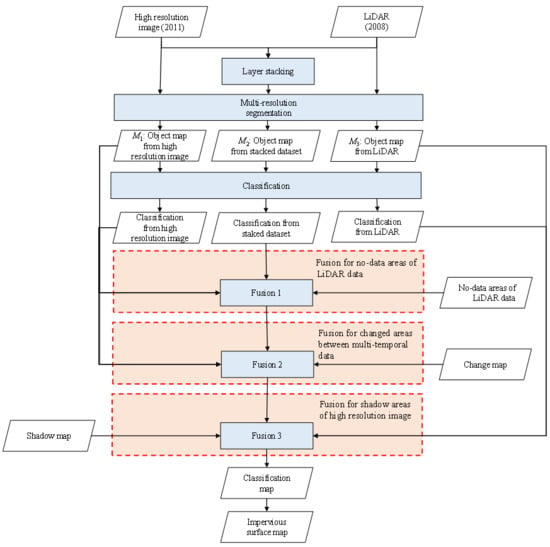
In this section, we will introduce the details of the proposed method. Most of the method’s procedures were coded while using the MATLABTM (MathWorks, Natick, MA, USA) platform, while the segmentation step was conducted using the eCognition DeveloperTM (Trimble Inc., Sunnyvale, CA, USA). The flowchart of the entire method is presented in Figure 3. The three maps for observation difference (i.e., change map, shadow map and no-data areas) were extracted from the high-resolution image and LiDAR data. The change detection approach for multi-sensor data is outlined in Section 3.3. The no-data map of LiDAR data was generated by thresholding the intensity of LiDAR data, while the shadow map is obtained by direct classification from the high-resolution image. Finally, the three observation difference maps and two multi-temporal data are used as the inputs of the object-based post-classification fusion process, which is detailed in Section 3.4. Across the whole procedure, segmentation is applied by means of multi-resolution segmentation (MRS), which is introduced in Section 3.1.
3.1. Segmentation
Object-based processing is very effective in the analysis and interpretation of high-resolution remote sensing data. Thus, we employ segmentation to produce homogeneous objects as the basic units. MRS is one of the most popular and effective segmentation algorithms. This algorithm is a bottom-up region-merging technique that is designed to form homogenous objects starting with single pixels [41]. The commercial software eCognition DeveloperTM, which embeds this algorithm, is employed in this study.
Apart from the segmentation with single-sensor data (i.e., the high-resolution image or LiDAR data) that is involved in the independent classification step, the segmentation object map that was produced while using both the stacked LiDAR data and the high-resolution image is also employed in both change detection and the post-classification steps. More specifically, the objects are formed according to the information derived from the stacked dataset; thus, the pixels within one object are temporally similar, meaning that they are all either changed or unchanged. Therefore, the changed areas can be identified as independent objects and will not be mixed with the unchanged areas. After segmentation, the feature value of one object is assigned as the mean value of all pixels inside.
3.2. Change Detection
In most previous studies, the high-resolution image is integrated with the LiDAR data directly, since the process operates under the assumption that the multi-sensor data provides information about the same landscape. However, when the multi-sensor data are acquired at different points in time, there will be numerous changes and observation differences spread across the whole image [46,47], which have been described in detail in Section 2. If these changes and observation differences are neglected, misclassification errors will be unavoidable, since the features of the corresponding areas are provided by different landscapes. Therefore, change detection between multi-temporal data was employed to distinguish between changed areas and mis-registration areas. Moreover, the shadow areas are extracted by the classification of the high-resolution image, while no-data areas are detected by thresholding the LiDAR data.
Since the feature bands of different sensor data are acquired by means of different observation mechanisms, post-classification is the most straightforward method through which to detect changes. In short, changed areas are directly detected by comparing the two independent classification results, which are themselves acquired from the corresponding single-sensor data. However, the accuracy of post-classification is mostly unsatisfactory in these cases, since classification that employs only single-sensor data can struggle to achieve good performance and will accumulate classification errors [48,49,50]. Moreover, it is worth noting that, although the feature bands are not the same, there will be correlations between the data from two different sensors for the same landscape. For example, grass (with its specific spectral signature) will show low elevation and high intensity in the LiDAR data, while a building (with a different spectral signature) will show high elevation and low intensity. Therefore, the idea behind direct change detection between multi-temporal and multi-sensor data involves finding the correlations between different features and detecting the anomalous changed objects.
Consequently, we employ the MAD algorithm in order to detect the changes between multi-temporal LiDAR data and the high-resolution image. The change detection procedure is presented in Figure 4. The stacked dataset is firstly segmented into object maps via MRS, which has been introduced in the previous section. After segmentation, the object is deemed the basic unit of the feature band; its value has been assigned as the mean of pixels within one object. The MAD algorithm is then employed in order to extract change information. Finally, the OTSU thresholding method is used to separate the changed areas.
MAD is derived from canonical correlation analysis and seeks to find the transformed features and maximize the variance of their difference. Mathematically, for two multi-temporal data X and Y, MAD aims to find transformation vectors a and b, so that:
under the constraints that and .
It can be observed from Equation (1), that, since the transformed vector for each data is different, MAD can deal with multi-sensor data and find the transformation feature space in order to analyze their correlation.
Thus, the optimization objective can be transformed into the following equation:
where maximizing the variance is the same as minimizing the correlation. This optimization problem can also be solved by calculating two generalized eigenvalue problems:
where , , and are the covariance matrix of X, Y and their interaction. After the transformation vectors are obtained, the difference of transformed features is used to detect changes.
The best change detection performance will be obtained by the transformed features with the maximum eigenvalue that is aimed at finding the maximum correlation between multi-temporal data. There will be some correlations between different features that are generated from different sensor images for the same landscape, and the real changes should appear anomalous relative to this correlation. Therefore, the MAD-transformed features will minimize the difference of observation features by maximizing the correlation of the unchanged landscapes; in this way, the real changes will be highlighted. Accordingly, in our experiment, the last MAD-transformed feature corresponding to the maximum eigenvalue is selected so as to distinguish the changed areas.
Although the unsupervised MAD can analyze the correlations among the entire set of data, the feature learning may be affected by changed areas. Training samples are necessary to facilitate the classification of different landscape classes. Thus, training samples from the unchanged areas in the multi-temporal LiDAR data and the high-resolution image can be used for transformation space learning. Subsequently, the transformed features of the entire dataset are calculated with the learned transformation vectors.
The difference of features corresponding to the maximum correlation is used to detect changes. Finally, the binary change map is automatically obtained by applying the OTSU thresholding method to the absolute difference image of the last MAD features.
3.3. Object-Based Post-Classification Fusion
After change detection is complete, the LiDAR data and the high-resolution image from a different acquisition time are integrated in order to map the impervious surface distribution, while taking the changes and observation differences into consideration. In order to achieve better fusion performance, an object-based post-classification fusion method (containing three main fusion steps) is proposed. This method considers the spatial information from the object map, which integrates the joint classification result for stacked multi-sensor data with the independent classification result for single-sensor data.
Generally, in most traditional approaches to the fusion of different types of data, some change areas or observation difference areas (such as shadows [51]) in one independent classification result yielded by the corresponding single image are directly filled using the results of another independent classification. However, this will not result in good performance, since independent classification that uses only single-sensor data is not very effective when dealing with a complex urban environment. Therefore, we propose a new object-based post-classification fusion method that solves the problems of real landscape changes and observation differences between multi-temporal LiDAR data and the high-resolution image by considering the spatial information from object maps. It is firstly worth noting that the changed areas and observation difference areas appear only in one image, not in both sets of multi-temporal data. For example, the no-data areas are only contained in the LiDAR data, while the high-resolution image can provide the hidden information inside these areas; moreover, the shadow areas appear only in the high-resolution image, while the LiDAR data can provide information regarding the detailed landscapes under shadows; finally, for the changed areas, the landscape class in the latest target data reflects the impervious surface mapping result at that time. Accordingly, the core idea behind object-based post-classification fusion involves taking advantage of joint classification results that are located in the neighbors of changed and observation difference areas to the greatest extent possible, according to the object spatial information.
Using the fusion for changed areas as an example in Figure 5, we regard the newly acquired high-resolution image (from the year 2011) as the target image. Since the target image is newer and its landscape is more accurate, the object map M1 is generated by the target image, which is used as the main input data for the fusion’s changed areas component. Generally, all the homogenous pixels within one object belong to the same class of landscape; this forms the core concept underpinning the illustration of the post-classification fusion procedure below. Moreover, the change map between multi-temporal LiDAR data and the high-resolution image is obtained while using the method that is outlined in Section 3.2. For an object in M1:
- if it is totally in the interior of the changed areas, its class can only be determined according to the independent classification result from the high-resolution image;
- if this object intersects with the changed areas, this means that the class type of this object should be consistent with the class type of the intersecting areas between this object and unchanged areas. Previous research has shown that joint classification using stacked LiDAR data and high-resolution imagery generally yields better performance than independent classification while using sole sensor data alone [37]. Thus, the class type of this object is determined by the class extracted from the joint classification result located in the intersection between unchanged areas and this object.
Ultimately, the object spatial information is used in this way during the class identification of the changed areas. The accurate classification result is thereby obtained and the completeness of the objects retained. Similarly, the fusion for no-data areas, shadows and mis-registration can be conducted along almost the same lines as described above, whereas the inputs object map and independent classification map are different from the two maps noted in Figure 5. The specific input maps of the fusion for no-data areas, shadows, and mis-registration are presented in Figure 6.
In summary, the procedure of the object-based post-classification fusion method is outlined in Figure 6 and will be subsequently described in more detail. Firstly, MRS is used to generate three object maps for the high-resolution image, LiDAR data, and the stacked dataset, respectively. After the object maps are generated, six features (mean, variance, shape index, length-width ratio, density, and roundness) [52] of each object are calculated and form the input of the next classification step. In addition to the six features, NDVI is also involved in the independent classification with high-resolution image. The NDVI feature band is stacked with six object features, which form the input for classification. Secondly, the stacked dataset of LiDAR data and high-resolution image is classified in order to obtain the joint classification map; the independent classification maps are also obtained via the corresponding single-sensor data. The same training samples are used in the three classification processes (the shadow class is not included only in the classification of LiDAR data). A support vector machine (SVM) with a Gaussian kernel is chosen as a classifier in this study due to its high performance when dealing with small samples [53]. Thirdly, the final classification result for the newer sensor data (i.e., the high-resolution image acquired in the year 2011) is produced through the three steps of the object-based post-classification fusion of the three classification results (one joint classification and two independent classifications), including the fusion for the no-data areas of LiDAR data, the real changed areas between the LiDAR data and high-resolution image resulting from their different acquisition times, and the shadow areas of the high-resolution image. Finally, the impervious surface map at the later time (i.e., the year 2011) is obtained via class merging with the final classification result.
The details of the three main fusion steps involved in Figure 6 are as follows:
- 1.
- Fusion for no-data areas of LiDAR data
There are some no-data areas in the LiDAR data, as shown in Figure 7b, which will lead to classification errors if not addressed. Accordingly, the first step in the object-based post-classification fusion is to acquire the correct classification result for the no-data areas in the LiDAR data. The no-data map of the LiDAR data was generated by thresholding. More specifically, the object map from the high-resolution image was employed, since the high-resolution image can provide accurate object spatial information for these no-data areas. It can be seen in Figure 7 that, although there are some no-data areas in the LiDAR data (Figure 7b), these should be located inside a building object according to the object map from the high-resolution image (Figure 7a,c), and the whole building object will belong to the same class type. Therefore, in the object-based post-classification process, we select an object that intersects with the no-data areas of the LiDAR data. The final classification result of the selected object is determined by means of major vote from the class types (extracted from the joint classification result) of all pixels whose value in the LiDAR data is positive and are also located in this object. However, if all the pixels within the selected object are designated no-data in the LiDAR data, the class type of this object is determined by means of independent classification with the high-resolution image alone.
- 2.
- Fusion for changed areas between multi-temporal LiDAR data and high-resolution image
Since the high-resolution image was acquired later than the LiDAR data, we use the high-resolution image as the target image in order to obtain the latest impervious surface map. The change map (including mis-registration areas) is obtained via the change detection method that is proposed in Section 3.2. The object map M1 of the high-resolution image is utilized for the purpose of considering the spatial and shape compactness of the landscape distribution (see Figure 8). According to the detailed description of Figure 5 that is provided above, if one object from M1 is located inside of the changed areas, the final class type should be assigned according to the independent classification result from the high-resolution image; for the unchanged areas, the class type is assigned according to the joint classification result. In addition, if the object has an intersection with both changed and unchanged areas, the class type of this object will be determined by a major vote of the joint classification results in unchanged areas. This is because any one object should be homogenous and belong to only one class of landscape. Moreover, in addition to the real landscape changes, mis-registration areas are also (technically) a type of change. Accordingly, mis-registration areas can also be detected by change detection, and the associated corrections will also be completed after this fusion step (see Figure 9).
- 3.
- Fusion for shadow areas of the high-resolution image
When determining the class of the landscape under the shadow areas using the LiDAR data and the high-resolution image, one direct method is to use the independent classification result from the LiDAR data to restore the class information. However, as discussed above, the independent classification is not as accurate as the joint classification. Therefore, we take advantage of the spatial object information obtained from LiDAR data by means of the proposed object-based post-classification fusion. As shown in Figure 10, there are no shadow problems in the LiDAR data in the same area. According to the object map M3 from the LiDAR data, the landscape under the shadows is generally related to the landscape near the shadow and belongs to the same class. More specifically, if both a shadow and a non-shadow area exist in the same object, the class type of the landscape under the shadow area is determined by major vote among all the class types (extracted from joint classification) in the non-shadow areas. Moreover, if the object is completely located within a shadow area, the class of this object is determined by means of the independent classification result while using LiDAR data alone. The shadow map used in this process is obtained from the independent classification of the high-resolution image.
It can be seen that these three steps all utilize the similar core concept that underpins the proposed object-based post-classification fusion. After the above three steps of the proposed object-based post-classification fusion are complete, the final classification result is acquired; this result considers the differences between the LiDAR data and the high-resolution image across different acquisition times and takes advantage of many features from the different sensor data. Lastly, the latest impervious surface map is generated via class merging that is based on the final classification.
3.4. Accuracy Assessment
Throughout the whole process, there are two process that produce maps, namely change detection and object-based post-classification fusion. Therefore, in order to evaluate the effectiveness of the proposed method, we will conduct an accuracy assessment for change detection and classification.
The change detection is evaluated while using a reference map, which contains labelled samples of changes and non-changes. Visual comparison and Kappa coefficient are used as metrics to prove the superior performance of the proposed change detection process.
The classification map is obtained after the object-based post-classification fusion. The reference map, marked with numerous labelled samples for all classes, is used for evaluation, and the overall accuracy (OA), Kappa coefficients, and confusion matrices are presented for assessment.
Finally, the impervious surface map that is generated by combining the classification maps is presented and quantitatively evaluated by confusion matrix.
4. Experiment
4.1. Change Detection
The high-resolution image and LiDAR data are stacked and segmented while using the MRS algorithm with the eCognition DeveloperTM. The segmentation parameters are set on the basis of visual interpretation in order to maintain the completeness of landscape objects: thus, scale is 20, weight of shape is 0.1, and weight of compactness is 0.5.
The training samples are selected manually for both change detection and classification. The samples contains 114 pixels for roof, 97 pixels for vegetation, 80 pixels for road and parking lots, 79 pixels for soil, 98 pixels for pavement, and 93 pixels for shadow. In change detection, five classes of training samples (excluding shadow) are used for training.
In this experiment, in addition to the proposed supervised MAD method (sp_MAD), we also use the unsupervised MAD (un_MAD), stack PCA (st_PCA) [54], and post-classification (post-class) [47,55] methods for comparison. Unsupervised MAD was used on the whole image to extract the correlations between multi-temporal data sets. PCA transformation was applied on the stacked dataset, and the change information was found in the 4th Principal Components (PCs). This is because information about the greater proportion of unchanged areas is concentrated in the top PCs, meaning that change information is highlighted in one of the remaining bands. However, the disadvantage of the stacked PCA method is that it can be hard to determine which band is useful for change detection. In this paper, the change information band of stack PCA is determined by means of visual interpretation. Post-classification is a classical change detection method that directly compares the class type of two independent classification results that were produced from the corresponding single-sensor data. If the class types of these two classification results are different, it means that a change has occurred, and vice versa.
The change intensity images for supervised MAD, unsupervised MAD, and stacked PCA are shown in Figure 11 and include the absolute values of feature bands with change information. Higher values indicate a higher possibility of change. To better illustrate the changes detected in the change intensity images, the change intensity image of supervised MAD and its corresponding areas in the high-resolution image and LiDAR data are presented in Figure 12, which contains (a) real landscape change, (b) mis-registration, (c) shadows, and (d) real landscape change. By combining Figure 11 and Figure 12, it can be observed that the proposed supervised MAD method has the ability to detect the changes and some observation differences in the multi-temporal LiDAR data and the high-resolution image. In the visual comparison, the areas featuring data change are better highlighted in the results of the supervised MAD than in those for the other two methods.
The binary change maps of supervised MAD, unsupervised MAD, stack PCA by OTSU thresholding method, and the binary change maps of the post-classification method are presented in Figure 13. Through visual interpretation, it can be observed that the supervised MAD detected fewer areas of change, while the other methods detected quite a number of changes covering the whole scene. Post-classification directly compares the class types of two corresponding independent classification results that were yielded by corresponding single-sensor data. If the two class types are different, these areas will be determined to be changed areas. Figure 13d shows that there are far more changed areas than unchanged areas, a result that is caused by the accumulation of independent classification errors in post-classification.
In order to carry out quantitative assessment, reference samples for change detection are selected, as shown in Figure 14. The reference samples contain 9449 changed pixels (in yellow) and 198,842 unchanged pixels (in green).
The quantitative evaluation is presented in Table 1. In order to reduce the influence of imbalance among the training samples, we used the Kappa coefficient. The maximum Kappa coefficients that can be obtained with all the possible thresholds in the absolute image (Figure 11) are listed in the last column of Table 1, while the current Kappa coefficients for the binary maps in Figure 13 are listed in the middle column. Two automatic thresholding methods are used in this paper, namely K-means clustering and OTSU thresholding. In order to make the proposed method more automatic, it is necessary to apply automatic thresholding for the binary change map. To avoid bias that is caused by automatic thresholding, we choose these two widely used thresholding methods and draw a comparison. The max Kappa indicates the best results that can be obtained by the experimental methods, while the current Kappa shows the accuracy of the results with the automatic thresholding method; the former indicates the change detection ability, while the latter indicates performance in real applications. The current Kappa coefficients are also the indicator to choose the automatic thresholding method.
It can thereby be seen that the post-classification method demonstrates extremely low accuracy; this is because the change detection accuracy is determined by the two independent classifications, each of which only use single-sensor data, meaning that the accuracy is limited. Among all the methods, the unsupervised MAD obtains the highest Max Kappa, while supervised MAD achieves obviously superior performance after automatic thresholding. This is because supervised MAD can improve the separability of changed areas, meaning that it is easier for the automatic thresholding method to find the optimum threshold. Meanwhile, the thresholding method of OTSU outperforms K-means, such that the binary change map that is produced by the former method is selected as the input of the change map in the subsequent fusion process.
4.2. Object-Based Post-Classification Fusion
In this paper, the main objective is to obtain the impervious surface distribution map for the newer target image, considering landscape changes and observation differences. Therefore, the high-resolution image from 2011 was used as the target image, while the LiDAR data from 2008 was used as the auxiliary data. For quantitative assessment, the reference maps for the 2011 high-resolution image are produced by visual interpretation and presented in Figure 15. In terms of test samples, roof samples are red (62,507 pixels), grass samples are green (46,923 pixels), road and parking lot samples are grey (58,337 pixels), soil samples are yellow (22,883 pixels), and pavement samples are cyan (17,440 pixels).
The classification results of independent classification, joint classification, and the proposed method are shown in Figure 16. The independent classification maps are obtained by means of object-based classification while using only the high-resolution image or LiDAR data. The joint classification map is obtained by classification using both the stacked high-resolution image and the LiDAR data. The final classification map is generated using the proposed method, as introduced in Section 3. In order to obtain a better result, the segmentation scale is set at 20 in the independent classifications of the LiDAR data and high-resolution image, while in the object-based post-classification fusion, the segmentation scale is set at 10 for more homogeneous objects. In Figure 16a, the results of independent classification using the high-resolution image show that the accuracy of building class is low and that there are many misclassification errors. The independent classification result while using LiDAR data (see Figure 16b) illustrates that, while the LiDAR data yields good performance on building classification, the pavement proves difficult to identify. Figure 16c,d both show accurate classification maps, although the joint classification map contains shadow areas, which will be removed after the object-based post-classification fusion. Meanwhile, in some building areas, the joint classification results show obvious misclassifications of buildings due to the no-data areas in the LiDAR data. These problems are mostly corrected after the proposed object-based post-classification fusion steps.
Table 2 presents the OAs and Kappa coefficients of the classification maps for the proposed method and the comparative methods. As the data shows, joint classification while using both LiDAR data and the high-resolution image performs better than each independent classification on its own. Moreover, the proposed method results in an obvious improvement due to its use of object-based post-classification fusion. Table 3, Table 4, Table 5 and Table 6 present the confusion matrices of the independent classification maps of both the high-resolution image and LiDAR data, the joint classification map, and the classification map that is generated while using the proposed method. ‘R&P’ in these tables indicates the class of ‘road and parking’. In Table 3 (high-resolution image), it can be seen that the buildings are mis-classified into road and parking, soil, and shadow. Mis-classification between soil and building is the main source of errors in impervious surface mapping. Comparatively, in Table 4 (LiDAR data), the soil is well-separated from the buildings, whereas the pavement is not well-separated from the soil. In Table 5 (joint classification), most landscapes are well classified, but suffer interference from shadows. Finally, in the results of the proposed method presented in Table 6, most pixels in the image can be seen to have been classified accurately. Most errors in impervious surface mapping while using this method occur during the identification of soil.
Table 7 shows the false alarm rate (FAR) [56] and omission rate (OR) of each class for the proposed method and the comparison methods. The numbers in bold indicate the highest accuracies (i.e., lowest rates of false alarms and omissions) for each class. For example, it can be observed that the independent classification of the high-resolution image cannot accurately distinguish between building and soil, while the LiDAR data also performs poorly when classifying soil and pavement. For its part, the joint classification (using both the high-resolution image and LiDAR data) achieves improvements across almost all classes when compared with the two independent classifications, which indicates the effectiveness of multi-sensor data classification. Most importantly, the proposed method obtains further improvements as compared with the joint classification, such as a lower omission rate of buildings and a lower false alarm rate for soil. Therefore, the proposed method can be seen to have the ability to obtain higher classification accuracy, as shown in Table 2.
In order to test the proposed object-based post-classification fusion strategy, we compare two approaches to fusing the independent classification results and the joint classification result. One is to fill the no-data areas, changed areas and shadow areas with the corresponding independent classification result directly, without considering the object spatial information. For instance, the independent classification result that is provided by the high-resolution image alone is used to fill the no-data areas in the LiDAR data. The other approach is to fuse the two independent classification results and the joint classification result while considering the object spatial information through the proposed object-based post-classification fusion strategy, which is described in Section 3.3. The bars in Figure 17 above provide a detailed illustration of the improvement after each fusion step with or without object spatial information. Since there are three fusion steps after the joint classification results that are obtained, the different colors in Figure 17 indicate the increase in accuracy after each step. Figure 17 illustrates that all of the proposed three main fusion steps can improve the classification accuracy. In addition, it can be seen that the fusion approach that incorporates object spatial information yields better performance than an approach that does not consider object spatial information. Thus, the proposed fusion approach, which considers the object spatial information, is most effective in improving the performance of the final classification map.
Figure 18, Figure 19 and Figure 20 present the improvements that are achieved by each main step in the proposed object-based post-classification fusion method. In Figure 18, as highlighted by the dark and red circles, there are many no-data areas for missing LiDAR data, which leads to obviously incorrect classification results. However, after the object-based post-classification fusion is complete (see Figure 18d), these areas are accurately corrected. Figure 19 shows the correction for changed areas, where there are obvious roof changes inside the circles. Before correction, areas had been falsely classified; after correction, the corresponding areas are correctly classified in the building class, which is the correct class in the newer high-resolution image (from 2011). Figure 20 shows the correction in shadow areas. Since there are many shadows in the high-resolution image, the shadowy regions of the landscapes are difficult to classify. After the proposed object-based post-classification fusion method is applied, however, the landscape inside the shadow areas can be identified while using multi-sensor data.
Finally, the impervious surface distribution map is obtained by combining the corresponding landscapes, as shown in Figure 21; here, the impervious surface is blue and the pervious surface is green. The impervious surface contains buildings, roads, parking lots, and pavement, while the other areas are pervious. It should be noted that this impervious surface distribution is very typical of American urban areas. Therefore, impervious surface distribution mapping is likely to be extremely useful in urban structure analysis and the corresponding hydrology or city planning study.
The confusion matrix and accuracy assessment are presented in Table 8. It can be observed that most impervious surface pixels are correctly labelled, with a producer accuracy of 95.08%. The overall accuracy is 95.6014% and the Kappa coefficient is 0.9029. These figures indicate that the proposed method can map the impervious surface accurately.
5. Discussion
5.1. Improvement over Independent Classification and Joint Classification
For detailed classification in the complex urban environment, it is difficult to obtain satisfactory accuracy while using only single-sensor data, such as single LiDAR data or an optical high-resolution image alone. The reasons for this include (1) the confusion between different landscapes in some observation information, such as the similar spectral values between roof and road, or similar density values between pavement and grass, and (2) the disturbance in single sensor data, such as shadows in high-resolution images, among other factors. By contrast, joint classification while using the stacked LiDAR data and high-resolution imagery utilizes multi-sensor data and makes use of abundant information from multiple physical characteristics. It can be seen from Table 7, that, when compared with independent classification, joint classification leads to lower FARs and ORs for almost all landscape classes. In particular, the joint classification yields a very low FAR when compared to that of the LiDAR data, and a very low FAR and OR as compared to that of the high-resolution image. This indicates that joint classification is able to take advantage of the information from multi-sensor data.
However, the joint classification with the multi-temporal stacked dataset also ignores the real landscape changes and observation differences. By contrast, the proposed method utilizes joint classification as the basis and then employs three main steps of object-based post-classification fusion when addressing these data problems. Visually, the proposed object-based post-classification fusion is evidently able to correct the classification results: see e.g., (1) the correction for the no-data areas, as shown in Figure 18; (2) the correction for the changed areas, as shown in Figure 19; and, (3) the correction for the shadow areas, as shown in Figure 20.
In quantitative assessment, if landscape changes and observation differences are considered, even without the object spatial information, classification accuracy (Kappa) can be improved from 0.8372 to 0.8723, as shown in Figure 17. By means of the proposed object-based post-classification fusion, the accuracy can be further improved to 0.8942. Figure 17 also illustrates that each fusion step works to solve the problems of landscape changes and observation differences. The result is a step-by-step increase in the final classification accuracy.
For the detailed landscape classes shown in Table 7, the proposed method obtains an obvious decrease in OR for the building class compared with the joint classification, since the no-data areas and shadow areas covering the buildings are corrected after the proposed fusion. Moreover, the decrease in the FAR for the soil class is mainly caused by the proposed fusion in no-data areas, since some of these areas are falsely classified as soil by the joint classification method. In addition, the obvious decrease in OR for the pavement class is due to class re-identification in shadowy areas, since most pavements are located beside the buildings, and are thus easily affected by the shadows cast by these structures.
Therefore, it can be concluded that it is necessary to consider landscape changes and observation difference when mapping impervious surfaces using LiDAR data and high-resolution images with difference acquisition time. The proposed method can obtain an obvious improvement when compared with joint classification.
5.2. Limitations
The proposed method integrates joint classification with independent classifications according to the segmentation object maps. It is worth noting that the improvement achieved by the proposed method is mainly based on the joint classification. Thus, if the joint classification cannot provide an accurate class map, the accuracy of the improved result will also be limited. Moreover, the proposed method also makes use of the independent classification results, the segmentation object maps, the extraction of landscape changes, and observation difference. Therefore, the error accumulation of all these processes will affect the performance of the proposed method.
When dealing with multi-sensor data, registration is one of the main pre-processing steps, and is thus also included in our pre-processing. While the proposed method does have the ability to extract some of the mis-registration areas via MAD change detection, it will cause many false alarms if the registration accuracy is relatively low. In addition, the orthorectification of the high-resolution image is also necessary in order to facilitate the fusion with the LiDAR data. After orthorectification and accurate registration is complete, the slight mis-registration for high buildings can be handled by the proposed method.
5.3. Future Work
Change detection between LiDAR data and high-resolution images with different acquisition times is an important step in extracting changed areas and mis-registration areas for fusion. In our future work, we want to develop a more accurate multi-sensor change detection method so as to detect changes between multi-temporal data.
In the proposed method, joint classification with stacked LiDAR data and high-resolution imagery is employed. In order to better explore the complementary information, the development of a new classification method that handles multi-sensor data is also one of the targets for our future work.
In our experiment, landscape changes were found to exist, but were not very common at the study site. In our future work, we want to collect LiDAR data and high-resolution images covering rapidly developing urban areas, such as cities in China. The effectiveness of the proposed method in conducting the latest impervious surface mapping will then be evaluated using LiDAR data and high-resolution images covering these areas at different acquisition times, meaning that there will be obvious urban expansion and change at the study site.
6. Conclusions
Impervious surface mapping is very important for the study of urban environments, since it is an indicator of city development. Impervious surface mapping while using multi-sensor data has been attracting increasing interest of late. However, when the multi-sensor data is acquired at different times, some real landscape changes and observation differences may exist between these data, which will lead to unavoidable misclassification errors and lower the final classification accuracy.
Mapping impervious surface with multi-sensor data can improve the performance upon single sensor data, whereas both real landscape changes and observance differences between the data need to be considered. In this paper we have identified four sources of potential errors between high resolution imagery and LiDAR data, and proposed an improved impervious surface mapping method to maximize the information content of the multi-sensor data sets while minimizing the introduced errors due to inconsistencies in the data. A multispectral high-resolution image and LiDAR data from the city of Buffalo were used in this study. The stacked data of the high-resolution image and the LiDAR data were firstly segmented into an object map while using the MRS algorithm to maintain the completeness of the landscape in classification. Supervised MAD and OTSU thresholding were then used to detect data changes by learning from the unchanged training samples. Finally, the core concept of the object-based post-classification fusion was proposed in order to take advantage of the joint classification map with the stacked dataset and independent classification maps with the single sensor data. The object information was utilized during the fusion to maintain the completeness of the landscape objects and improve the classification accuracy. After classification was complete, the impervious surface map at the later time was generated by merging the roof, road, parking lot, and pavement classes.
In the experiment, a study site in Buffalo was selected to demonstrate the effectiveness of our proposed method. The main problems to consider were real landscape changes, no-data areas in LiDAR data, mis-registration, and shadow areas in the high-resolution image. The experiment demonstrates that the supervised MAD method can yield better change detection results than post-classification change detection and other unsupervised methods. With the automatically obtained binary change detection result, the final land-cover maps that were generated by our proposed method show an obvious improvement compared with joint classification and the independent classifications. Moreover, the experiments indicate that the proposed object-based post-classification fusion, which considers object spatial information, results in better performance when compared to simply filling the areas with independent classification results.
Our study demonstrates that it is necessary to consider landscape changes and observation differences during the fusion of LiDAR data and high-resolution images with different acquisition times. Given the continuing development of multi-sensor remote sensing observation, our proposed method has the potential to be used for detailed impervious surface mapping, updating, and real-time monitoring in urban environments using the newest single-sensor data and historical different-sensor data.
Author Contributions
H.L. had the original idea for this study, conducted the experiments, and wrote the manuscript. L.W. revised the manuscript and provided guidance on the overall research. C.W. provided some ideas about the change detection method. L.Z. provided some revision comments for this manuscript.
Funding
This research was funded by [the National Natural Science Foundation of China] grant number [41801285 and 61601333], [Open Research Fund of Key Laboratory of Digital Earth Science, Institute of Remote Sensing and Digital Earth, Chinese Academy of Sciences] grant number [2017LDE003], [Open Research Project of The Hubei Key Laboratory of Intelligent Geo-Information Processing] grant number [KLIGIP-2017B05], and [Fundamental Research Founds for National University, China University of Geosciences (Wuhan)] grant number [G1323541864].
Conflicts of Interest
The authors declare no conflict of interest.
References
- Arnold, C.L., Jr.; Gibbons, C.J. Impervious surface coverage: The emergence of a key environmental indicator. J. Am. Plan. Assoc. 1996, 62, 243–258. [Google Scholar] [CrossRef]
- Hu, X.; Weng, Q. Impervious surface area extraction from IKONOS imagery using an object-based fuzzy method. Geocarto Int. 2011, 26, 3–20. [Google Scholar] [CrossRef]
- Zhang, L.; Weng, Q. Annual dynamics of impervious surface in the Pearl River Delta, China, from 1988 to 2013, using time series Landsat imagery. ISPRS J. Photogramm. Remote Sens. 2016, 113, 86–96. [Google Scholar] [CrossRef]
- Weng, Q. Modeling urban growth effects on surface runoff with the integration of remote sensing and GIS. Environ. Manag. 2001, 28, 737–748. [Google Scholar] [CrossRef]
- Weng, Q. Remote sensing of impervious surfaces in the urban areas: Requirements, methods, and trends. Remote Sens. Environ. 2012, 117, 34–49. [Google Scholar] [CrossRef]
- Hurd, J.D.; Civco, D.L. Temporal characterization of impervious surfaces for the state of Connecticut. In Proceedings of the ASPRS Annual Conference, Denver, CO, USA, 23–28 May 2004. [Google Scholar]
- Harbor, J.M. A practical method for estimating the impact of land-use change on surface runoff, groundwater recharge and wetland hydrology. J. Am. Plan. Assoc. 1994, 60, 95–108. [Google Scholar] [CrossRef]
- Yuan, F.; Bauer, M.E. Comparison of impervious surface area and normalized difference vegetation index as indicators of surface urban heat island effects in Landsat imagery. Remote Sens. Environ. 2007, 106, 375–386. [Google Scholar] [CrossRef]
- Schueler, T.R. The importance of imperviousness. Watershed Prot. Technol. 1994, 1, 100–111. [Google Scholar]
- Xian, G.; Homer, C. Updating the 2001 National Land Cover Database impervious surface products to 2006 using Landsat imagery change detection methods. Remote Sens. Environ. 2010, 114, 1676–1686. [Google Scholar] [CrossRef]
- Wang, Q.; Meng, Z.; Li, X. Locality adaptive discriminant analysis for spectral-spatial classification of hyperspectral images. IEEE Geosci. Remote Sens. Lett. 2017, 14, 2077–2081. [Google Scholar] [CrossRef]
- Shi, C.; Wang, L. Linear spatial spectral mixture model. IEEE Trans. Geosci. Remote Sens. 2016, 54, 3599–3611. [Google Scholar] [CrossRef]
- Wang, Q.; Zhang, F.; Li, X. Optimal clustering framework for hyperspectral band selection. IEEE Trans. Geosci. Remote Sens. 2018, PP, 1–13. [Google Scholar] [CrossRef]
- Slonecker, E.T.; Jennings, D.B.; Garofalo, D. Remote sensing of impervious surfaces: A review. Remote Sens. Rev. 2001, 20, 227–255. [Google Scholar] [CrossRef]
- Shao, Z.; Liu, C. The integrated use of DMSP-OLS nighttime light and MODIS data for monitoring large-scale impervious surface dynamics: A case study in the Yangtze river delta. Remote Sens. 2014, 6, 9359–9378. [Google Scholar] [CrossRef]
- Deng, C.; Wu, C. A spatially adaptive spectral mixture analysis for mapping subpixel urban impervious surface distribution. Remote Sens. Environ. 2013, 133, 62–70. [Google Scholar] [CrossRef]
- Flanagan, M.; Civco, D.L. Subpixel impervious surface mapping. In Proceedings of the 2001 ASPRS Annual Convention, Louis, MO, USA, 23–27 April 2001. [Google Scholar]
- Wu, C. Normalized spectral mixture analysis for monitoring urban composition using ETM+ imagery. Remote Sens. Environ. 2004, 93, 480–492. [Google Scholar] [CrossRef]
- Lu, D.; Weng, Q. Use of impervious surface in urban land-use classification. Remote Sens. Environ. 2006, 102, 146–160. [Google Scholar] [CrossRef]
- Wu, C.; Murray, A.T. Estimating impervious surface distribution by spectral mixture analysis. Remote Sens. Environ. 2003, 84, 493–505. [Google Scholar] [CrossRef]
- Zhou, Y.; Wang, Y.Q. Extraction of impervious surface areas from high spatial resolution imagery by multiple agent segmentation and classification. Photogramm. Eng. Remote Sens. 2008, 74, 857–868. [Google Scholar] [CrossRef]
- Yuan, F.; Bauer, M.E. Mapping impervious surface area using high resolution imagery: A comparison of object-based and per pixel classification. In Proceedings of the ASPRS 2006 Annual Conference, Reno, NV, USA, 1–5 May 2006. [Google Scholar]
- Li, P.J.; Guo, J.C.; Song, B.Q.; Xiao, X.B. A multilevel hierarchical image segmentation method for urban impervious surface mapping using very high-resolution imagery. IEEE J. Sel. Top. Appl. Earth Obs. Remote Sens. 2011, 4, 103–116. [Google Scholar] [CrossRef]
- Huang, X.; Zhang, L.; Gong, W. Information fusion of aerial images and LiDAR data in urban areas: Vector-stacking, re-classification and post-processing approaches. Int. J. Remote Sens. 2011, 32, 69–84. [Google Scholar] [CrossRef]
- Yan, W.Y.; Shaker, A.; El-Ashmawy, N. Urban land cover classification using airborne LiDAR data: A review. Remote Sens. Environ. 2015, 158, 295–310. [Google Scholar] [CrossRef]
- Zhang, J.; Lin, X. Advances in fusion of optical imagery and LiDAR point cloud applied to photogrammetry and remote sensing. Int. J. Image Data Fusion 2017, 8, 1–31. [Google Scholar] [CrossRef]
- Zhang, J. Multi-source remote sensing data fusion: Status and trends. Int. J. Image Data Fusion 2010, 1, 5–24. [Google Scholar] [CrossRef]
- Guo, T.; Yasuoka, Y. Snake-based approach for building extraction from high-resolution satellite images and height data in urban areas. In Proceedings of the 23rd Asian Conference on Remote Sensing, Kathmandu, Nepal, 25–29 November 2002. [Google Scholar]
- Wang, R. 3D building modeling using images and LIDAR: A review. Int. J. Image Data Fusion 2013, 4, 273–292. [Google Scholar] [CrossRef]
- Meng, X.; Wang, L.; Silván-Cárdenas, J.L.; Currit, N. A multi-directional ground filtering algorithm for airborne LiDAR. ISPRS J. Photogramm. Remote Sens. 2009, 64, 117–124. [Google Scholar] [CrossRef]
- Guo, B.; Huang, X.; Zhang, F.; Sohn, G. Classification of airborne laser scanning data using JointBoost. ISPRS J. Photogramm. Remote Sens. 2015, 100, 71–83. [Google Scholar] [CrossRef]
- Lafarge, F.; Descombes, X.; Zerubia, J.; Pierrot-Deseilligny, M. Automatic building extraction from DEMs using an object approach and application to the 3D-city modeling. ISPRS J. Photogramm. Remote Sens. 2008, 63, 365–381. [Google Scholar] [CrossRef] [Green Version]
- Yang, B.; Dong, Z.; Zhao, G.; Dai, W. Hierarchical extraction of urban objects from mobile laser scanning data. ISPRS J. Photogramm. Remote Sens. 2015, 99, 45–57. [Google Scholar] [CrossRef]
- Zhou, W.; Troy, A. An object-oriented approach for analyzing and characterizing urban landscape at the parcel level. Int. J. Remote Sens. 2008, 29, 3119–3135. [Google Scholar] [CrossRef]
- Guo, L.; Chehata, N.; Mallet, C.; Boukir, S. Relevance of airborne LiDAR and multispectral image data for urban scene classification using random forests. ISPRS J. Photogramm. Remote Sens. 2011, 66, 56–66. [Google Scholar] [CrossRef]
- Zhou, W. An object-based approach for urban land cover classification: Integrating LiDAR height and intensity data. IEEE Geosci. Remote Sens. Lett. 2013, 10, 928–931. [Google Scholar] [CrossRef]
- Hodgson, M.E.; Jensen, J.R.; Tullis, J.A.; Riordan, K.D.; Archer, C.M. Synergistic use of LiDAR and color aerial photography for mapping urban parcel imperviousness. Photogramm. Eng. Remote Sens. 2003, 69, 973–980. [Google Scholar] [CrossRef]
- Im, J.; Lu, Z.Y.; Rhee, J.; Quackenbush, L.J. Impervious surface quantification using a synthesis of artificial immune networks and decision/regression trees from multi-sensor data. Remote Sens. Environ. 2012, 117, 102–113. [Google Scholar] [CrossRef]
- Hartfield, K.A.; Landau, K.I.; Leeuwen, W.J.D.V. Fusion of high resolution aerial multispectral and LiDAR data: Land cover in the context of urban mosquito habitat. Remote Sens. 2011, 3, 2364–2383. [Google Scholar] [CrossRef]
- Yu, B.; Liu, H.; Zhang, L.; Wu, J. An object-based two-stage method for a detailed classification of urban landscape components by integrating airborne LiDAR and color infrared image data: A case study of downtown Houston. In Proceedings of the 2009 Joint Urban Remote Sensing Event, Shanghai, China, 20–22 May 2009. [Google Scholar]
- Benz, U.C.; Hofmann, P.; Willhauck, G.; Lingenfelder, I.; Heynen, M. Multi-resolution, object-oriented fuzzy analysis of remote sensing data for GIS-ready information. ISPRS J. Photogramm. Remote Sens. 2004, 58, 239–258. [Google Scholar] [CrossRef] [Green Version]
- Nielsen, A.A.; Conradsen, K.; Simpson, J.J. Multivariate alteration detection (MAD) and MAF postprocessing in multispectral, bitemporal image data: New approaches to change detection studies. Remote Sens. Environ. 1998, 64, 1–19. [Google Scholar] [CrossRef]
- Canty, M.J.; Nielsen, A.A. Automatic radiometric normalization of multitemporal satellite imagery with the iteratively re-weighted MAD transformation. Remote Sens. Environ. 2008, 112, 1025–1036. [Google Scholar] [CrossRef] [Green Version]
- Nielsen, A.A. The regularized iteratively reweighted MAD method for change detection in multi- and hyperspectral data. IEEE Trans. Image Process. 2007, 16, 463–478. [Google Scholar] [CrossRef] [PubMed]
- Otsu, N. A threshold selection method from gray-level histograms. Automatica 1975, 11, 23–27. [Google Scholar] [CrossRef]
- Wu, C.; Zhang, L.; Du, B. Kernel slow feature analysis for scene change detection. IEEE Trans. Geosci. Remote Sens. 2017, 55, 2367–2384. [Google Scholar] [CrossRef]
- Wu, C.; Du, B.; Cui, X.; Zhang, L. A post-classification change detection method based on iterative slow feature analysis and Bayesian soft fusion. Remote Sens. Environ. 2017, 199, 241–255. [Google Scholar] [CrossRef]
- Coppin, P.; Jonckheere, I.; Nackaerts, K.; Muys, B.; Lambin, E. Digital change detection methods in ecosystem monitoring: A review. Int. J. Remote Sens. 2004, 25, 1565–1596. [Google Scholar] [CrossRef]
- Lu, D.; Mausel, P.; Brondizio, E.; Moran, E. Change detection techniques. Int. J. Remote Sens. 2004, 25, 2365–2401. [Google Scholar] [CrossRef]
- Singh, A. Review article digital change detection techniques using remotely-sensed data. Int. J. Remote Sens. 1989, 10, 989–1003. [Google Scholar] [CrossRef]
- Zhou, W.; Huang, G.; Troy, A.; Cadenasso, M. Object-based land cover classification of shaded areas in high spatial resolution imagery of urban areas: A comparison study. Remote Sens. Environ. 2009, 113, 1769–1777. [Google Scholar] [CrossRef]
- Definiens Professional 5 Reference Book. 2006. Available online: http://read.pudn.com/downloads112/sourcecode/others/467350/eCognition5.0%20ReferenceBook.pdf (accessed on 14 June 2018).
- Suykens, J.A.K.; Vandewalle, J. Least squares support vector machine classifiers. Neural Process. Lett. 1999, 9, 293–300. [Google Scholar] [CrossRef]
- Collins, J.B.; Woodcock, C.E. An assessment of several linear change detection techniques for mapping forest mortality using multitemporal Landsat TM data. Remote Sens. Environ. 1996, 56, 66–77. [Google Scholar] [CrossRef]
- Li, H.; Xiao, P.; Feng, X.; Yang, Y.; Wang, L.; Zhang, W.; Wang, X.; Feng, W.; Chang, X. Using land long-term data records to map land cover changes in china over 1981–2010. IEEE J. Sel. Top. Appl. Earth Obs. Remote Sens. 2017, 10, 1372–1389. [Google Scholar] [CrossRef]
- Wu, C.; Du, B.; Zhang, L. A subspace-based change detection method for hyperspectral images. IEEE J. Sel. Top. Appl. Earth Obs. Remote Sens. 2013, 6, 815–830. [Google Scholar] [CrossRef]
Figure 1.
Study site: Buffalo, NY, USA.

Figure 2.
The changes and observation difference between the multi-temporal high-resolution image and light detection and ranging (LiDAR) data are highlighted by red circles or polygons, and all LiDAR data is displayed in pseudo-color raster image (red band and blue band: normalized Digital Surface Model (nDSM), green band: intensity). Above: (a) high-resolution image after changes; (b) LiDAR data before changes; (c) high building in the high-resolution image with mis-registration; (d) high building in the LiDAR data with mis-registration; (e) high-resolution image without missing data; (f) LiDAR data with missing data; (g) high-resolution image with shadows; and, (h) LiDAR data without shadows.

Figure 3.
Flowchart of the proposed method. The multi-sensor data acquired at different time were process by change detection to obtain the change map. The shadow map and no-data areas of LiDAR data were obtained separately. Finally, the multi-source data were interpreted by the proposed object-based post-classification fusion with the shadow map, change map, and no-data areas. The accurate impervious surface map was generated for the result.

Figure 4.
Flowchart of change detection with multi-temporal LiDAR data and high-resolution image. The multi-sensor data were firstly stacked and segmented by multi-resolution segmentation (MRS) algorithm. The object based data were processed by multivariate alteration detection (MAD) algorithm and OTSU thresholding to obtain the binary change map.

Figure 5.
Diagram for the object-based post-classification fusion. If the object is totally in the interior of the changed area, its class type is determined with the independent classification result. Otherwise, if the object intersects with the changed area, its class type is determined mainly while considering the joint classification result in the unchanged area.

Figure 6.
Flowchart of object-based post-classification fusion of multi-temporal LiDAR data and the high-resolution image. The joint classification and independent classification results are obtained at first. Then, three steps of object-based post-classification fusion is achieved to obtain the accurate classification map. The impervious surface map is obtained by merging the classes.

Figure 7.
The spatial correspondences for the no-data area between multi-temporal LiDAR data and the high-resolution image: (a) high-resolution image; (b) LiDAR data; and, (c) mask for no-data area. The red rectangle indicates the schematic object from the high-resolution image.
Figure 7.
The spatial correspondences for the no-data area between multi-temporal LiDAR data and the high-resolution image: (a) high-resolution image; (b) LiDAR data; and, (c) mask for no-data area. The red rectangle indicates the schematic object from the high-resolution image.

Figure 8.
The spatial correspondence for the changed areas between multi-temporal LiDAR data and the high-resolution image: (a) high-resolution image; (b) LiDAR data; and, (c) mask for changed area. The red rectangle indicates the schematic object from the high-resolution image.
Figure 8.
The spatial correspondence for the changed areas between multi-temporal LiDAR data and the high-resolution image: (a) high-resolution image; (b) LiDAR data; and, (c) mask for changed area. The red rectangle indicates the schematic object from the high-resolution image.

Figure 9.
The spatial correspondence for the mis-registration areas between multi-temporal LiDAR data and the high-resolution image: (a) high-resolution image; (b) LiDAR data; and, (c) mask for no-data area. The red rectangle indicates the schematic object from the high-resolution image.
Figure 9.
The spatial correspondence for the mis-registration areas between multi-temporal LiDAR data and the high-resolution image: (a) high-resolution image; (b) LiDAR data; and, (c) mask for no-data area. The red rectangle indicates the schematic object from the high-resolution image.

Figure 10.
The spatial correspondence for the shadow areas between multi-temporal LiDAR data and the high-resolution image: (a) high-resolution image; (b) LiDAR data; and, (c) mask for shadow areas. The red rectangle indicates the schematic object from the LiDAR data.
Figure 10.
The spatial correspondence for the shadow areas between multi-temporal LiDAR data and the high-resolution image: (a) high-resolution image; (b) LiDAR data; and, (c) mask for shadow areas. The red rectangle indicates the schematic object from the LiDAR data.

Figure 11.
Change intensity images obtained by (a) supervised MAD, (b) unsupervised MAD, and (c) stack PCA. Higher values in the image indicate the higher probability to be changed. The four red rectangles and yellow labels indicate the zoomed areas shown in Figure 12 below.
Figure 11.
Change intensity images obtained by (a) supervised MAD, (b) unsupervised MAD, and (c) stack PCA. Higher values in the image indicate the higher probability to be changed. The four red rectangles and yellow labels indicate the zoomed areas shown in Figure 12 below.

Figure 12.
The change intensity image of supervised MAD (greyscale image), and its corresponding areas in the high-resolution image (true color image) and LiDAR data (pseudo-color image). The cases shown above are (a) real landscape change, (b) mis-registration, (c) shadows, and (d) another real landscape change. Higher values of the change intensity indicate the high probability to be changed.

Figure 13.
Binary change maps by OTSU of (a) supervised MAD, (b) unsupervised MAD, (c) stack PCA, and (d) the binary change maps of post-classification, where the changed areas are white and the unchanged areas are black.
Figure 13.
Binary change maps by OTSU of (a) supervised MAD, (b) unsupervised MAD, (c) stack PCA, and (d) the binary change maps of post-classification, where the changed areas are white and the unchanged areas are black.

Figure 14.
Reference samples for change detection. Changed/unchanged samples are labelled in yellow/green, respectively.
Figure 14.
Reference samples for change detection. Changed/unchanged samples are labelled in yellow/green, respectively.

Figure 15.
Reference map for the high-resolution image taken in 2011. The legends indicate the colors in the image.
Figure 15.
Reference map for the high-resolution image taken in 2011. The legends indicate the colors in the image.

Figure 16.
(a) Independent classification map of high-resolution image, (b) independent classification map of LiDAR data, (c) joint classification map using LIDAR data and high-resolution image, and (d) classification map following object-based post-classification fusion (the proposed method).
Figure 16.
(a) Independent classification map of high-resolution image, (b) independent classification map of LiDAR data, (c) joint classification map using LIDAR data and high-resolution image, and (d) classification map following object-based post-classification fusion (the proposed method).

Figure 17.
Classification accuracies with different fusion approaches. Different colors indicate the increased accuracies after each step of object-based post-classification fusion.
Figure 17.
Classification accuracies with different fusion approaches. Different colors indicate the increased accuracies after each step of object-based post-classification fusion.

Figure 18.
Fusion for no-data areas of LiDAR data: (a) high-resolution image, (b) LiDAR data, (c) joint classification map using LiDAR data and high-resolution image before object-based post-classification fusion, and (d) classification map after object-based post-classification fusion.
Figure 18.
Fusion for no-data areas of LiDAR data: (a) high-resolution image, (b) LiDAR data, (c) joint classification map using LiDAR data and high-resolution image before object-based post-classification fusion, and (d) classification map after object-based post-classification fusion.

Figure 19.
Fusion for changed areas between multi-temporal data: (a) high-resolution image, (b) LiDAR data, (c) joint classification map using LiDAR data and high-resolution image before object-based post-classification fusion, and (d) classification map after object-based post-classification fusion.

Figure 20.
Fusion for shadow areas of high-resolution image: (a) high-resolution image, (b) LiDAR data, (c) joint classification map using LiDAR data and high-resolution image before object-based post-classification fusion, and (d) classification map after object-based post-classification fusion.
Figure 20.
Fusion for shadow areas of high-resolution image: (a) high-resolution image, (b) LiDAR data, (c) joint classification map using LiDAR data and high-resolution image before object-based post-classification fusion, and (d) classification map after object-based post-classification fusion.

Figure 21.
Impervious surface distribution map in 2011.


Table 1.
Max Kappa and current Kappa for supervised MAD and comparative methods.
| Current Kappa | Max Kappa | ||
|---|---|---|---|
| K-Means | OTSU | ||
| sp_MAD | 0.5187 | 0.6419 | 0.7440 |
| un_MAD | 0.1901 | 0.2328 | 0.7550 |
| stack_PCA | 0.2003 | 0.2524 | 0.6881 |
| post-class | 0.1409 | ||
Table 2.
Quantitative assessment of classification maps for the proposed method and the comparison methods. The reference is shown as Figure 15. The values in the table indicate the overall accuracy and Kappa coefficient.
Table 2.
Quantitative assessment of classification maps for the proposed method and the comparison methods. The reference is shown as Figure 15. The values in the table indicate the overall accuracy and Kappa coefficient.
| High-Resolution Image | LiDAR Data | Joint Classification | Proposed Method | |
|---|---|---|---|---|
| OA (%) | 77.30 | 77.80 | 87.49 | 91.89 |
| Kappa | 0.6999 | 0.7128 | 0.8372 | 0.8942 |
Table 3.
Confusion matrix of the high-resolution image classification map, where the reference is shown as Figure 15. The values in the table indicate the numbers of pixels.
Table 3.
Confusion matrix of the high-resolution image classification map, where the reference is shown as Figure 15. The values in the table indicate the numbers of pixels.
| Building | Vegetation | R&P | Soil | Pavement | Shadow | Total | |
|---|---|---|---|---|---|---|---|
| Building | 39,401 | 18 | 10,862 | 6653 | 1758 | 3815 | 62,507 |
| Vegetation | 122 | 46,289 | 0 | 321 | 82 | 109 | 46,923 |
| R&P | 13,432 | 17 | 37,133 | 3977 | 3277 | 501 | 58,337 |
| Soil | 6220 | 29 | 529 | 15,300 | 513 | 292 | 22,883 |
| Pavement | 3340 | 54 | 586 | 874 | 11,957 | 629 | 17,440 |
| Total | 62,515 | 46,407 | 49,110 | 27,125 | 17,587 | 5346 |
Table 4.
Confusion matrix of the LiDAR data classification map, where the reference is shown as Figure 15. The values in the table indicate the numbers of pixels.
Table 4.
Confusion matrix of the LiDAR data classification map, where the reference is shown as Figure 15. The values in the table indicate the numbers of pixels.
| Building | Vegetation | R&P | Soil | Pavement | Total | |
|---|---|---|---|---|---|---|
| Building | 47,471 | 1106 | 11,364 | 619 | 1947 | 62,507 |
| Vegetation | 381 | 39,748 | 6 | 2296 | 4492 | 46,923 |
| R&P | 527 | 2728 | 48,608 | 2835 | 3639 | 58,337 |
| Soil | 376 | 493 | 2876 | 16,747 | 2391 | 22,883 |
| Pavement | 470 | 303 | 1487 | 4594 | 10,586 | 17,440 |
| Total | 49,225 | 44,378 | 64,341 | 27,091 | 23,055 |
Table 5.
Confusion matrix of the joint classification map, where the reference is shown as Figure 15. The values in the table indicate the numbers of pixels.
Table 5.
Confusion matrix of the joint classification map, where the reference is shown as Figure 15. The values in the table indicate the numbers of pixels.
| Building | Vegetation | R&P | Soil | Pavement | Shadow | Total | |
|---|---|---|---|---|---|---|---|
| Building | 46,926 | 21 | 9792 | 902 | 887 | 3979 | 62,507 |
| Vegetation | 302 | 45,605 | 16 | 94 | 439 | 467 | 46,923 |
| R&P | 601 | 2 | 48,523 | 6073 | 1756 | 1382 | 58,337 |
| Soil | 419 | 24 | 618 | 20,751 | 364 | 707 | 22,883 |
| Pavement | 504 | 131 | 1120 | 1045 | 13,815 | 825 | 17,440 |
| Total | 48,752 | 45,783 | 60,069 | 28,865 | 17,261 | 7360 |
Table 6.
Confusion matrix for the proposed method, where the reference is shown as Figure 15. The values in the table indicate the numbers of pixels.
Table 6.
Confusion matrix for the proposed method, where the reference is shown as Figure 15. The values in the table indicate the numbers of pixels.
| Building | Vegetation | R&P | Soil | Pavement | Total | |
|---|---|---|---|---|---|---|
| Building | 58,002 | 246 | 2426 | 899 | 934 | 62,507 |
| Vegetation | 34 | 46,051 | 36 | 121 | 681 | 46,923 |
| R&P | 2997 | 6 | 50,182 | 3259 | 1893 | 58,337 |
| Soil | 438 | 24 | 678 | 21,267 | 476 | 22,883 |
| Pavement | 406 | 201 | 1011 | 1133 | 14,689 | 17,440 |
| Total | 61,877 | 46,528 | 54,333 | 26,679 | 18,673 |
Table 7.
False alarm rate (FAR) and omission rate (OR) of each class for the proposed method and the comparison methods. Bold numbers indicate the lowest rates of false alarms and omissions for each class.
Table 7.
False alarm rate (FAR) and omission rate (OR) of each class for the proposed method and the comparison methods. Bold numbers indicate the lowest rates of false alarms and omissions for each class.
| High-Resolution Image | LiDAR Data | Joint Classification | Proposed Method | |||||
|---|---|---|---|---|---|---|---|---|
| FAR (%) | OR (%) | FAR (%) | OR (%) | FAR (%) | OR (%) | FAR (%) | OR (%) | |
| Building | 31.13 | 26.68 | 3.36 | 24.23 | 3.75 | 19.82 | 5.00 | 5.48 |
| Vegetation | 0.50 | 0.63 | 10.97 | 23.63 | 0.39 | 1.83 | 1.10 | 1.96 |
| Soil | 39.39 | 44.22 | 30.53 | 23.24 | 28.11 | 6.43 | 5.01 | 13.87 |
| Pavement | 17.34 | 35.17 | 56.40 | 29.83 | 19.96 | 16.85 | 23.39 | 7.11 |
| Road & Parking | 26.48 | 24.39 | 25.32 | 16.17 | 19.22 | 14.80 | 21.91 | 16.09 |
Table 8.
Confusion matrix and accuracy of the impervious surface distribution map.
| Impervious | Pervious | Total (Reference) | |
|---|---|---|---|
| Impervious | 131,480 | 2349 | 13,3829 |
| Pervious | 6804 | 67,457 | 74,261 |
| Total (Test) | 138,284 | 69,806 | 208,090 |
| Overall Accuracy | 95.6014% | ||
| Kappa | 0.9029 |
© 2018 by the authors. Licensee MDPI, Basel, Switzerland. This article is an open access article distributed under the terms and conditions of the Creative Commons Attribution (CC BY) license (http://creativecommons.org/licenses/by/4.0/).
Share and Cite
MDPI and ACS Style
Luo, H.; Wang, L.; Wu, C.; Zhang, L. An Improved Method for Impervious Surface Mapping Incorporating LiDAR Data and High-Resolution Imagery at Different Acquisition Times. Remote Sens. 2018, 10, 1349. https://doi.org/10.3390/rs10091349
AMA Style
Luo H, Wang L, Wu C, Zhang L. An Improved Method for Impervious Surface Mapping Incorporating LiDAR Data and High-Resolution Imagery at Different Acquisition Times. Remote Sensing. 2018; 10(9):1349. https://doi.org/10.3390/rs10091349
Chicago/Turabian StyleLuo, Hui, Le Wang, Chen Wu, and Lei Zhang. 2018. "An Improved Method for Impervious Surface Mapping Incorporating LiDAR Data and High-Resolution Imagery at Different Acquisition Times" Remote Sensing 10, no. 9: 1349. https://doi.org/10.3390/rs10091349
Note that from the first issue of 2016, this journal uses article numbers instead of page numbers. See further details here.