Estimation of Terrestrial Global Gross Primary Production (GPP) with Satellite Data-Driven Models and Eddy Covariance Flux Data

Abstract

We estimate global terrestrial gross primary production (GPP) based on models that use satellite data within a simplified light-use efficiency framework that does not rely upon other meteorological inputs. Satellite-based geometry-adjusted reflectances are from the MODerate-resolution Imaging Spectroradiometer (MODIS) and provide information about vegetation structure and chlorophyll content at both high temporal (daily to monthly) and spatial (∼1 km) resolution. We use satellite-derived solar-induced fluorescence (SIF) to identify regions of high productivity crops and also evaluate the use of downscaled SIF to estimate GPP. We calibrate a set of our satellite-based models with GPP estimates from a subset of distributed eddy covariance flux towers (FLUXNET 2015). The results of the trained models are evaluated using an independent subset of FLUXNET 2015 GPP data. We show that variations in light-use efficiency (LUE) with incident PAR are important and can be easily incorporated into the models. Unlike many LUE-based models, our satellite-based GPP estimates do not use an explicit parameterization of LUE that reduces its value from the potential maximum under limiting conditions such as temperature and water stress. Even without the parameterized downward regulation, our simplified models are shown to perform as well as or better than state-of-the-art satellite data-driven products that incorporate such parameterizations. A significant fraction of both spatial and temporal variability in GPP across plant functional types can be accounted for using our satellite-based models. Our results provide an annual GPP value of ∼140 Pg C year${}^{-1}$ for 2007 that is within the range of a compilation of observation-based, model, and hybrid results, but is higher than some previous satellite observation-based estimates.

1. Introduction

Global terrestrial gross primary productivity (GPP), the amount of carbon dioxide (CO${}_2$) that is assimilated by plants through photosynthesis, plays a critical role in the global carbon cycle as it can moderate the amount of CO${}_2$ from anthropogenic sources that remains in the atmosphere. Despite the collection of ground-based data at hundreds of individual sites, as well as vast amounts of remotely-sensed data from satellites and the development of sophisticated process-based models, there still remains significant uncertainty in global GPP estimates including their global annual mean and inter-annual variability (IAV) [1]. Estimation of the variability in the land sink for global carbon budget assessments relies upon dynamic global vegetation models that are driven by observed environmental changes [2]. Peters et al. [3] note that the understanding of the land sink is currently limited in part by a dearth of spatially-explicit observations of vegetation changes and recommend systematic benchmarking of the models, including productivity, for improvement.

GPP is not measured directly either at the ground or from satellite. Using the eddy covariance technique, tower-based measurements of net ecosystem exchange (NEE) are partitioned into GPP and ecosystem respiration using assumptions regarding the latter (e.g., [1,4,5] and references therein). Despite the assumptions used in this approach, tower-based estimates are considered a standard for GPP estimates. Approaches to scale up these measurements and extrapolate globally involve first deriving relationships between tower-based GPP estimates and parameters from satellite-based instruments and meteorological analyses and then applying these parameterizations globally (e.g., [6,7,8,9,10]). Tramontana et al. [9] demonstrated that such approaches that use only remotely-sensed data perform almost as well as the best model that also incorporates meteorological inputs.

Other data-driven approaches to estimate GPP globally use satellite data in combination with models and various assumptions (see for comprehensive reviews [1,11]). Many of these are based on the light-use efficiency (LUE) concept [12,13], i.e.,

$$\mathrm{GPP}=\mathrm{LUE}\times {\mathrm{FAPAR}}_{\mathrm{chl}}\times {\mathrm{PAR}}_{\mathrm{in}},$$

(1)

where PAR${}_{\mathrm{in}}$ is photosynthetically-active radiation incident at the top of canopy and FAPAR${}_{\mathrm{chl}}$ is the fraction of PAR${}_{\mathrm{in}}$ absorbed by chlorophyll. Several studies have used the LUE model with space-based estimates of FAPAR${}_{\mathrm{chl}}$ or a proxy such as from satellite-derived vegetation indices (VI), PAR${}_{\mathrm{in}}$ estimates from a data assimilation system or other measurements, and parameterizations of LUE that use meteorological data as inputs to estimate GPP globally or on a smaller scale (e.g., [14,15,16,17,18,19,20,21]).

VIs are computed with a limited number of broad-band channels on satellite imagers. VIs that have been used or considered for estimating GPP include the dual wavelength Normalized Difference Vegetation Index (NDVI) [22] and the Near-Infrared Reflectance of terrestrial Vegetation (NIR${}_V$) [23] that is defined as the product of NDVI and reflectance from the near-infrared channel used in the NDVI. The potential benefit of using VIs for GPP estimation is that they can be simply derived from satellite reflectances. In particular, an NDVI record is available for over three decades [24].

VIs have been used to compute GPP with an approximation to Equation (1), i.e.,

$$\mathrm{GPP}=S\times \mathrm{VI}\times {\mathrm{PAR}}_{\mathrm{in}}$$

(2)

(e.g., [25]) or other similar forms (e.g., [26]) where VI is used as a proxy for FAPAR${}_{\mathrm{chl}}$. LUE, here represented as S, may be treated a constant [27,28] or as a more complex function of VI itself [29,30] or other parameters where S may vary with plant functional type (PFT) (e.g., [31]). Many of these approaches use flux tower data to train or calibrate their models with a limited number of sites or PFTs and have not been tested globally.

Some of the noted problems using VIs are (1) a decrease in sensitivity at high values, particularly in managed croplands (e.g., [25,32]) and (2) a positive offset that occurs when photosynthetic activity should be very low or zero (e.g., [20,26,33,34]) (i.e., these parameters have positive values when photosynthesis is not occurring). Yuan et al. [35] found that LUE models in general tended to overestimate GPP at low values and underestimate at high values and that most LUE models do not account for the fact that LUE is higher on cloudy days with more diffuse radiation (e.g., and references therein [36]). However, some LUE model formulations have included the radiation effect on LUE [37,38].

Gitelson et al. [39] and Peng et al. [40] found that the use of potential PAR (PAR${}_{\mathrm{pot}}$, i.e., the PAR at top of canopy that would be present in a cloudless atmosphere) in a simple model, i.e.,

$$\mathrm{GPP}\propto \mathrm{VI}\times {\mathrm{PAR}}_{\mathrm{pot}},$$

(3)

produced superior results as compared with PAR${}_{\mathrm{in}}$ in cropland vegetation. The improvement obtained by the use of PAR${}_{\mathrm{pot}}$ in place of PAR${}_{\mathrm{in}}$ with constant LUE implicitly accounts for the diffuse radiance effect on LUE by producing an effectively higher LUE at lower values of PAR${}_{\mathrm{in}}$. Peng et al. [40] notes that this model does not account for variations in GPP produced by short time scale (minutes to hours) stresses. They also suggested testing of this model at other geographic locations and for other vegetation types.

Here, we expand on this approach by training and evaluating models based on Equations (2) and (3) with available global GPP estimates from flux tower observations. We then test the satellite-based trained model using independent global GPP from flux towers (i.e., not used in the training). This is a simple and computationally-efficient method to estimate global GPP with a limited number of remotely-sensed parameters with a focus of daily to monthly time scales. We specifically examine whether a modified function of NDVI or a linear combination of band reflectances can accurately represent FAPAR${}_{\mathrm{chl}}$ to mitigate the above-mentioned shortcomings of VIs.

We further explore whether satellite measurements of chlorophyll solar-induced fluorescence (SIF) may be used to improve estimation of global GPP. SIF originates from the photosynthetic machinery inside leaves and has been measured with several satellite instruments [41,42,43,44,45,46,47,48]. The spectrum of chlorophyll fluorescence is spread over a range of wavelengths with two broad peaks, centered near 685 and 740 nm, referred to as the red and far-red emissions, respectively. Radiative transfer and physiological modeling suggests that canopy-level far-red SIF is strongly related to APAR [49]. Most satellite SIF studies have been conducted using far-red SIF, and henceforth, in this work, SIF will refer to far-red SIF. Several studies have shown a highly linear relationship between far-red canopy-level SIF and GPP on monthly time scales [32,46,50,51,52,53,54] that can be explained by modeling results [55]. Far-red SIF also closely follows seasonal [33] and daily to diurnal [54,56] variations in GPP. SIF measurements also alleviate the above-mentioned short-comings of VIs [32,33,57]. However, unlike VIs, SIF is a very small and difficult to measure signal. As a result, satellite SIF measurements are relatively noisy, prone to systematic errors [44,50,58] and currently limited in terms of both spatial and temporal resolution.

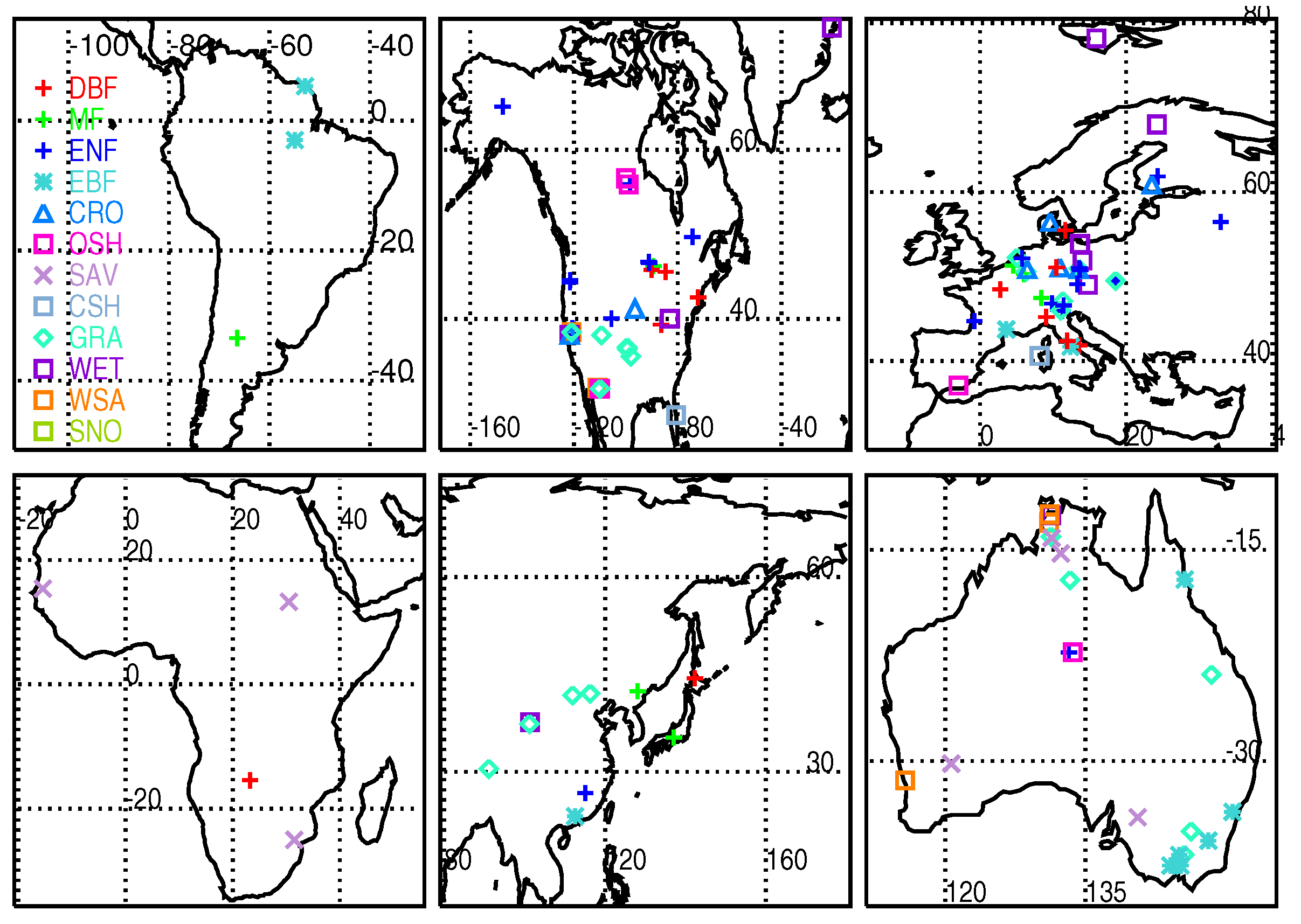
Here, we use attributes of both satellite-based reflectances and SIF in a computationally-efficient way to estimate global GPP accurately at high temporal and spatial resolution. In doing so, we seek to address the question: How much of the variance in GPP can be explained with satellite-derived quantities using a simple observation-based approach, particularly in comparison with more sophisticated approaches? To answer this question, we use GPP estimates derived at eddy covariance flux tower stations from the FLUXNET 2015 database to both calibrate and evaluate our satellite-based models. The results are examined at various temporal and spatial resolutions. We also compare with other data-driven GPP estimates and proxies as benchmarks. This comparison provides some insights into which parameters may be important for machine learning (ML) GPP estimates and ultimately may be used to improve the ML results.

2. Materials and Methods

2.1. MODIS Reflectances and Related Vegetation Parameters

The MODerate-resolution Imaging Spectroradiometer (MODIS) flies on the National Aeronautics and Space Administration (NASA) Earth Observing System (EOS) Terra (morning overpass) and Aqua (early afternoon overpass) polar-orbiting satellites. MODIS bandwidths for Channels 1–7 used here are 620–670 (red), 841–876 (near infrared 1, NIR${}_1$), 459–479 (blue), 545–565 (green), 1230–1250 (NIR${}_2$), 1628–1652 (short-wave infrared 1, SWIR${}_1$) and 2105–2155 nm (SWIR${}_2$), respectively. We primarily use the collection 6 MCD43D Nadir Bidirectional Reflectance Distribution Function (BRDF)-Adjusted Reflectance (NBAR) on a high resolution grid of 0.00833${}^{\circ }$ latitude × 0.00833${}^{\circ }$ longitude. MCD43D uses data acquired over a 16-day period at multiple angles for clear skies. Daily gridded reflectances are based on the 16-day periods and weight the data as a function of quality, observation coverage and temporal distance from the day of interest. These data are derived using a kernel-driven semi-empirical BRDF model [59,60,61]. Other MODIS data products examined here, such as different reflectance datasets, composited NDVI, FAPAR (or FPAR) and GPP estimates, are described in Appendix A.

2.1.1. Calculations of and Adjustments to Vegetation Indices

The NDVI and NIR${}_V$ (Normalized Difference Vegetation or Infrared Indices) are computed from MODIS Band 1 and 2 reflectances ($\rho$) using:

$$\mathrm{NDVI}=\frac{{\rho }_2-{\rho }_1}{{\rho }_2+{\rho }_1},$$

(4)

and:

$${\mathrm{NIR}}_V=(\mathrm{NDVI}-C)\times {\rho }_2,$$

(5)

where C is set to 0.08 as in Badgley et al. [23].

As noted above, the NDVI offsets at low values (denoted here as $N_0$) are presumably the result of non-chlorophyll-containing substances that produce a positive NDVI when photosynthesis or GPP is at or near zero. The chlorophyll-containing vegetation fraction (f) occupying a given satellite pixel increases during the growing season along with the NDVI. Therefore, subtracting a constant at all values of NDVI to reduce the offset may produce a corresponding underestimate at high values. Instead, we compute an adjusted NDVI according to NDVI${}^{\prime }$ = NDVI − NDVI${}_0$ where NDVI${}_0$ decreases linearly with NDVI from $N_0$ to zero as NDVI increases from $N_0$ (at $f=0$) to >$N_1$ (at $f=1$), i.e.,

$${\mathrm{NDVI}}_0=\left\{\begin{array}{cc}\mathrm{NDVI}\hfill & NDVI<N_0\hfill \\ \frac{(\mathrm{NDVI}-N_0)*-N_0}{(N_1-N_0)}+N_0\hfill & N_0<NDVI<N_1\hfill \\ 0\hfill & \mathrm{NDVI}>N_1\hfill \end{array}\right.$$

(6)

An expectation is that $N_0$ and perhaps $N_1$ vary with location. Satellite SIF measurements are near or at zero when GPP is near zero (e.g., [33]) and therefore offer the potential to map N${}_0$ globally. We attempted to derive spatially-varying $N_0$ using coincident observations of NDVI and satellite-based SIF. SIF data are only available with good temporal resolution at fairly low spatial resolution (∼0.5${}^{\circ }$). We applied standard least-squares fitting for grid boxes with sufficient seasonal variability in f. In this approach, we set $N_1$ to an empirically-derived constant value of 0.75. In the end, we obtained improved results using a constant value of $N_0=0.25$ rather than site-specific $N_0$ derived with SIF data. Therefore, for the remainder of the paper, we use $N_0=0.25$ and $N_1=0.75$ to compute NDVI${}^{\prime }$ according to Equation (6). It is hoped that improved results may be obtained in the future with higher spatial resolution and higher quality SIF data.

2.1.2. Use of Linear Combinations of Bands as an FAPAR${}_{\mathrm{chl}}$ Proxy

In place of VIs or modified VIs in Equations (1) or (2), we alternatively use the form:

$${\mathrm{FAPAR}}_{\mathrm{chl}}\propto (A_0+\sum _{i=1}^N{A}_i{\rho }_i),$$

(7)

where i is a particular reflectance band, N is the number of bands considered and ${\rho }_i$ are combined using weights $A_i$ and an offset $A_0$. [62] similarly used a neural network to estimate a SIF-based FAPAR${}_{\mathrm{chl}}$ proxy using MODIS reflectances. We examine the results below applied to GPP estimation for two different combinations of MODIS bands: (1) Bands 1 and 2 (red and NIR${}_1$) that are used to compute NDVI and NIR${}_V$ and (2) Bands 1–7 that are generally used for terrestrial remote sensing. Note that from MODIS, the first two bands are measured at ∼250 m, while the second group is measured at ∼500 m. Bands 1 and 2 or similar bands are also available on a number of other satellite sensors, such as the Advanced Very-High Resolution Radiometer (AVHRR) dating back to the early 1980s (albeit at lower spatial resolution than MODIS) and very high spatial resolution imagers such as on the Landsat and Sentinel 2 satellites. The additional MODIS bands may be useful for further removal of signals from non-chlorophyll-containing substances or atmospheric effects, as well as for noise reduction in the case of redundant information.

2.2. FLUXNET 2015

FLUXNET 2015 is a collection of eddy covariance flux data from multiple regional networks [63] that is an extension of the FLUXNET La Thuile dataset (2007). It includes improvements to the data quality control protocols and the data processing pipeline and the use of reanalysis data to fill gaps in micrometeorological variable records. Figure 1 shows maps of the flux tower sites used in this study that include only Tier 1 data open and free for scientific use. A listing of each site used in this study is provided in the Appendix B.

There are two main ways to estimate GPP (in units of g C m${}^{-2}$ d${}^{-1}$) by partitioning of the NEE computed with the variable Ustar (u${}^{*}$) threshold (VUT): (1) night-time method (GPP_NT_VUT_REF) [5]; and (2) day-time method (GPP_DT_VUT_REF)[4]. All results shown here use an average of night- and day-time partitioning methods. We repeated all analyses with each method separately and found that the conclusions did not differ significantly depending on which method was used. We use daily (DD, calculated from half-hourly data) and monthly (MM, average from daily data) files. We also made use of the short-wave (SW) incoming (IN) flux (SW_IN_F) and potential (top of atmosphere, SW_IN_POT), both in W m${}^{-2}$, provided in the dataset.

We apply quality control similar to that in previous works [10]. We use only daily or monthly averages where 20% or less have come from gap-filled data. We also use only data where the NEE uncertainties provided in the FLUXNET 2015 dataset are <3 g C m${}^{-2}$ d${}^{-1}$. Finally, we remove data points where the day-time and night-time partitioning results in GPP estimates that differ by more than 3 g C m${}^{-2}$ d${}^{-1}$. Data processing methods are described at http://fluxnet.fluxdata.org/data/fluxnet2015-dataset/data-processing/.

Total uncertainty in derived GPP includes gap-filling, partitioning uncertainty, random uncertainty and threshold friction velocity uncertainty [64]. Following Joiner et al. [33], we compute uncertainties in 8-day GPP flux tower-derived data (${\sigma }_{\mathrm{GPPtot}}$) according to:

$${\sigma }_{\mathrm{GPPtot}}=0.5085e^{0.1088*{\mathrm{GPP}}_{8\mathrm{day}}}.$$

(8)

This formulation is based on a general fitting to data from the AmeriFlux network of flux measurements spanning the Americas. For the sample of 8-day data that meet all the criteria, this produces a mean uncertainty estimate of ∼0.86 g C m${}^{-2}$ d${}^{-1}$. Assuming that random uncertainties can be reduced by averaging and that random uncertainty represents 50% of the total uncertainty consistent with Schaefer et al. [64], the uncertainties for monthly and daily data will be ∼0.68 and 1.8 g C m${}^{-2}$ d${}^{-1}$, respectively.

2.3. Satellite SIF and SIF-Based Downscaled Products

We use Version 27 (v27) Level 3 (gridded) SIF derived from the Global Ozone Monitoring Experiment 2 (GOME-2) onboard the MetOp-A (GOME-2A) from February 2007–December 2016 [43,44]. MetOp-A is in a polar orbit with an Equator crossing time of 09:30. The native spatial resolution of the GOME-2A data from launch to the middle of July 2013 was 40 × 80 km. From that time until the present, the resolution has been 40 × 40 km. GOME-2A provides global coverage in approximately 1–3 days. Here, we use SIF derived from the far-red fitting window: 734–758 nm. SIF is a very small signal (typically < a few mW/m${}^2$/nm/sr). Spatial and temporal averaging is employed to increase SIF signal-to-noise ratios (SNRs).

The quality control filters for GOME-2 Level 3 SIF are described in Joiner et al. [44]. GOME-2 SIF data with effective cloud fractions <30% are gridded monthly at $0.5^{\circ }\times 0.5^{\circ }$ resolution. This cloud screening is less rigorous as compared with that applied to MODIS data. GOME-2 retrievals of canopy-level SIF, which utilize the filling-in of solar Fraunhofer lines, are themselves not as greatly affected by clouds as are vegetation indices such as the NDVI [65]. However, top-of-atmosphere (TOA) SIF is affected by clouds in that it is sensitive to both the amount of solar radiation reaching the surface, as well as the amount of SIF that reaches the satellite. Therefore, TOA SIF should be reduced by approximately the square of the cloud transmittance as compared with the value in clear skies assuming that SIF yield remains constant with cloud conditions. Frankenberg et al. [66] showed that a substantial fraction of the canopy SIF can be detected by satellite for small to moderate cloud optical thicknesses.

Duveiller and Cescatti [67] implemented a method to downscale SIF with higher resolution MODIS data. Their approach used NDVI, as well as land surface temperature and evapotranspiration derived from MODIS to downregulate how much SIF is related to NDVI (or FAPAR). This product, referred to here as SIF*, is provided from 2007–2013 at a monthly timescale on a $0.{05}^{\circ }$×$0.{05}^{\circ }$ grid. Version 1 (v1) SIF* uses GOME-2 SIF Version 25 as an input. It should be noted that since v1 was produced, there have been two updates to the GOME-2 SIF data culminating in v27. These later versions used the same first step retrievals, but addressed various biases as identified by Köhler et al. [58] by applying posterior adjustments [44]. To obtain a monthly full-day estimate of SIF* from the original observations near 09:30 local time, we first divide each monthly grid box value of SIF* by the monthly-averaged top-of-atmosphere PAR (PAR${}_{\mathrm{TOA}}$) at 09:30, then multiply by monthly-averaged daily PAR${}_{\mathrm{TOA}}$ [68].

2.4. State-of-the-Art Satellite-Derived GPP Estimates

As benchmarks for comparison, we use two state-of-the-art data-driven global GPP estimates. FLUXCOM-RS is based on the global upscaling of flux tower data using satellite remotely-sensed (RS) data (no meteorological data) with a machine learning approach [6,7,10]. The product is generated at $0.{0833}^{\circ }\times 0.{0833}^{\circ }$ spatial and 8-day temporal resolution. It uses flux tower GPP with an ensemble of machine learning-based models and over 200 explanatory variables.

The Vegetation Photosynthesis Model (VPM) V20 [15,21,69,70,71] is based on the LUE approach and utilizes many remotely-sensed and climate reanalysis datasets. Different from the MODIS MOD17 GPP product, it uses a linear transformation of the Enhanced Vegetation Index (EVI) as a proxy of FAPAR${}_{\mathrm{chl}}$ (i.e., FAPAR${}_{\mathrm{chl}}$=1.25 [EVI-0.1]); the maximum LUE only differs for C3 and C4 plants, which is supported by a convergence of LUE when using this FAPAR${}_{\mathrm{chl}}$ [72]. VPM provides data at various resolutions. Here, we use monthly gridded data at $0.{05}^{\circ }\times 0.{05}^{\circ }$ resolution.

2.5. Sampling the FLUXNET 2015 Datasets for Training and Evaluation

In this work, we examine how well global GPP estimated from flux towers can be explained using simple relationships with satellite-based observations. Here, we use flux tower-derived GPP estimates to both calibrate and evaluate a variety of models. We use half of the available observations for calibration (i.e., deriving slopes between various satellite-based products and GPP) and the other half (independent) for evaluation of the derived relationships. We split the data alphabetically, i.e., according to the flux site name (even- or odd-numbered flux tower sites). In this way, half the sites are used for training and the other half for independent evaluation. This sorting selects sites such that if there are two (or more) sites per country, one site will be used for training and the other for evaluation. It also eliminates the possibility of data from a single site being included in both training and evaluation samples. This leads to more independence between the training and evaluation datasets. We find that results are similar, although not identical, depending on which half is used for training and that all general conclusions hold no matter which half of the sites is used for training.

In order to test GPP models on a wide range of conditions and plant functional types, we use all flux tower sites except for 23 identified by Zhang et al. [21] as having incompatibility with MODIS pixels and a few more additional sites at coastlines where FLUXCOM-RS did not produce good values. Each site was checked visually with MODIS 5km data. Sites were retained if the land cover and vegetation condition within the flux tower footprint (assumed 250-m radius) was similar (≥80%) to that within the overlapping MODIS data. All analyses are conducted for years 2003–2014 when FLUXNET 2015 and high quality MODIS data from both the Terra and Aqua satellites are available.

2.6. Statistical Parameters Used for Evaluation of Models

We evaluate different models on the basis of various statistical parameters including the root-mean squared error (RMSE) of the fit to the flux tower-based GPP, the variance explained ($r^2$), and the bias. As in Tramontana et al. [10], we use the model efficiency factor (MEF), a measure of how well our model reproduces independent data as compared with the mean value of observations, defined as:

$$\mathrm{MEF}=1-\frac{{\sum }_{i=1}^n{(x_i-y_i)}^2}{{\sum }_{i=1}^n{(y_i-\overline{y})}^2},$$

(9)

where $y_i$ and $x_i$ are the observed and fitted values, respectively, and $\overline{y}$ is the mean of $y_i$. Values of MEF > 0 indicate that the model used is better than the mean, and a value of unity would indicate a perfect model. We also use the metric $\lambda$ developed by Duveiller et al. [73], defined as:

$$\lambda =1-\frac{{\sum }_{i=1}^n{(x_i-y_i)}^2}{{\sum }_{i=1}^n{(x_i-\overline{x})}^2+{\sum }_{i=1}^n{(y_i-\overline{y})}^2+n(\overline{x}-\overline{y})+\kappa }$$

(10)

where $\kappa =0$ if $r\ge 0$ and $\kappa =2|{\sum }_{i=1}^n(x_i-\overline{x})(y_i-\overline{y})|$ if $r<0$. This index is equal to the correlation coefficient r when $r\ge 0$ and there is no additive or multiplicative bias and will be less than r in the presence of a bias. $\lambda$ has the advantage of summarizing the agreement in a single metric irrespective of whether any disagreement is due to lack of correlation or to a bias.

2.7. Data Processing Flow

A basic flow diagram of the training and evaluation using the various datasets is shown in Figure 2. The details involved in each of the processing steps will be described in more detail below. The datasets, with spatial and temporal resolutions listed in

Table 1. Summary of input datasets used for GPP estimation and evaluation with their native spatial and temporal resolutions (Res.).

Input Dataset	Temporal Res.	Spatial Res.
MCD43D reflectances ${}^a$	daily	$0.{0083}^{\circ }\times 0.{0083}^{\circ }$
GOME-2 SIF * ${}^b$	monthly	$0.{05}^{\circ }\times 0.{05}^{\circ }$
GOME-2 SIF ${}^c$	monthly	$0.5^{\circ }\times 0.5^{\circ }$
VPM GPP ${}^d$	monthly	$0.{05}^{\circ }\times 0.{05}^{\circ }$
FLUXCOM GPP ${}^d$	8 day	$0.{083}^{\circ }\times 0.{083}^{\circ }$
NIR${}_V$× SW${}_{\mathrm{TOA}}$ ${}^{b,e}$	any of the above	any of the above
NDVI × SW${}_{\mathrm{TOA}}$ ${}^{b,e}$	any of the above	any of the above
FLUXNET 2015 GPP ${}^f$	daily, monthly	site footprint

${}^a$ Used to compute FAPAR proxies such as NDVI, NIR${}_V$ and linear combinations of channels; ${}^b$ used as a GPP proxy with optional LUE parameterization; ${}^c$ used to identify highly productive regions optionally; ${}^d$ used for benchmark evaluation; ^e computed using MCD43D reflectance dataset; ${}^f$ half of sites used for training, the other half used for independent evaluation.

, may be grouped into several distinct subsets: (1) reflectances used to compute VIs (MCD43); (2) radiation, TOA short-wave (SW${}_{\mathrm{TOA}}$); (3) FLUXNET 2015 eddy covariance GPP estimates, half used for training and the other half for evaluation; (4) SIF (used to delineate highly productive regions) or downscaled SIF (SIF* used as a GPP proxy); (5) independent satellite data-driven GPP estimates used as benchmarks (VPM and FLUXCOM-RS). Further details on other datasets examined are given in Appendix A.

3. Results and Discussion

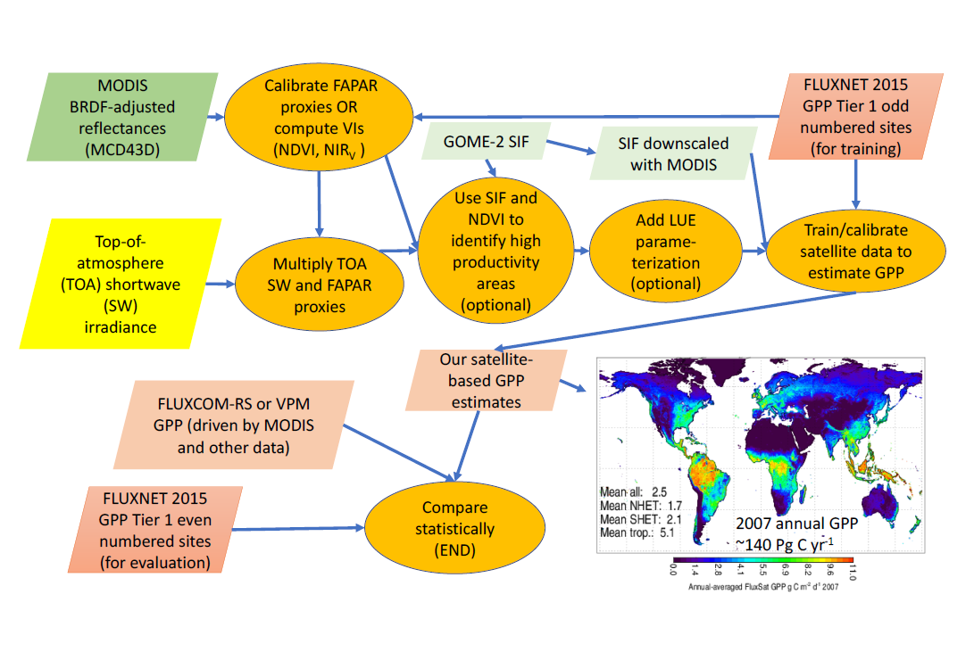
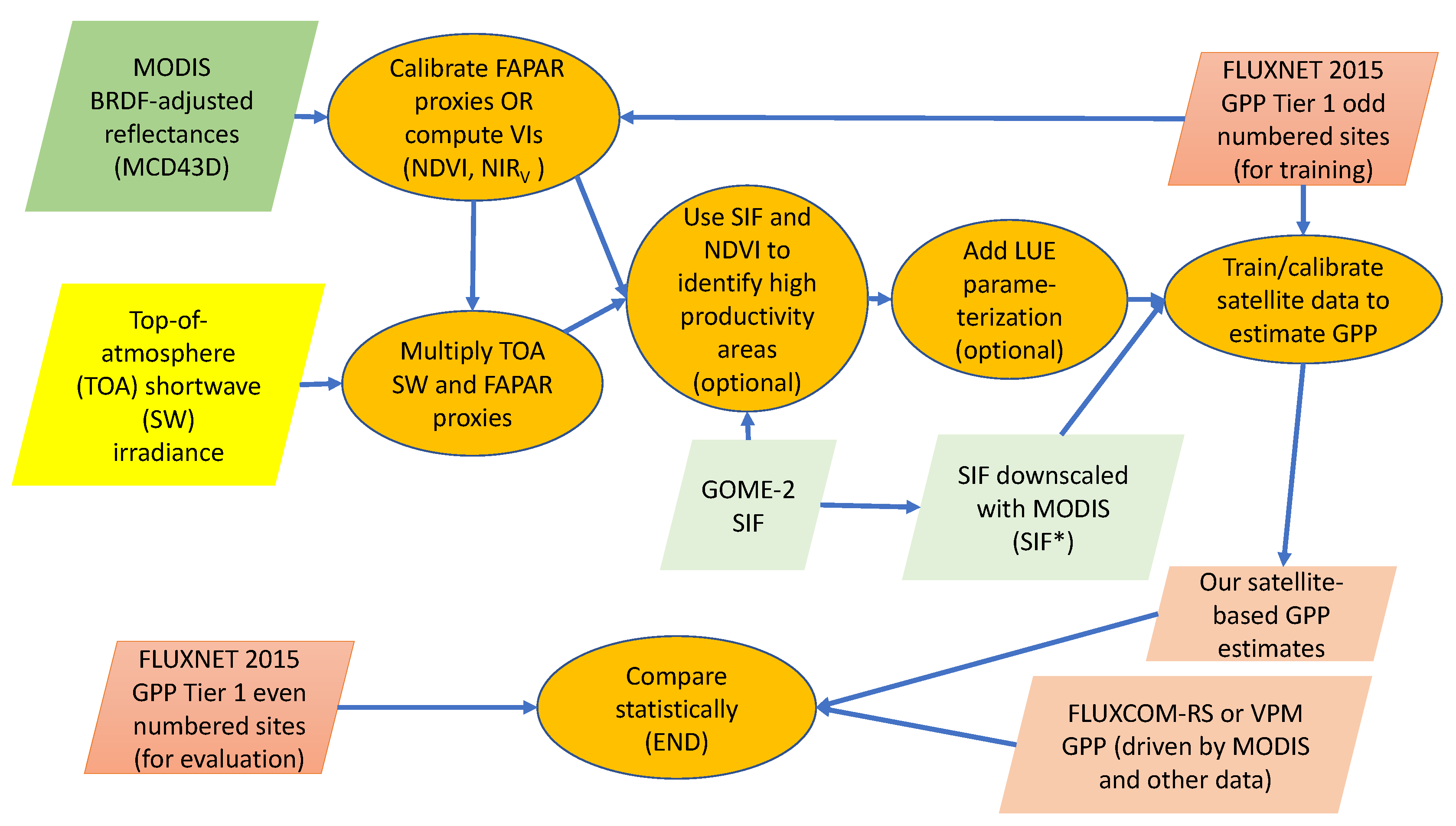
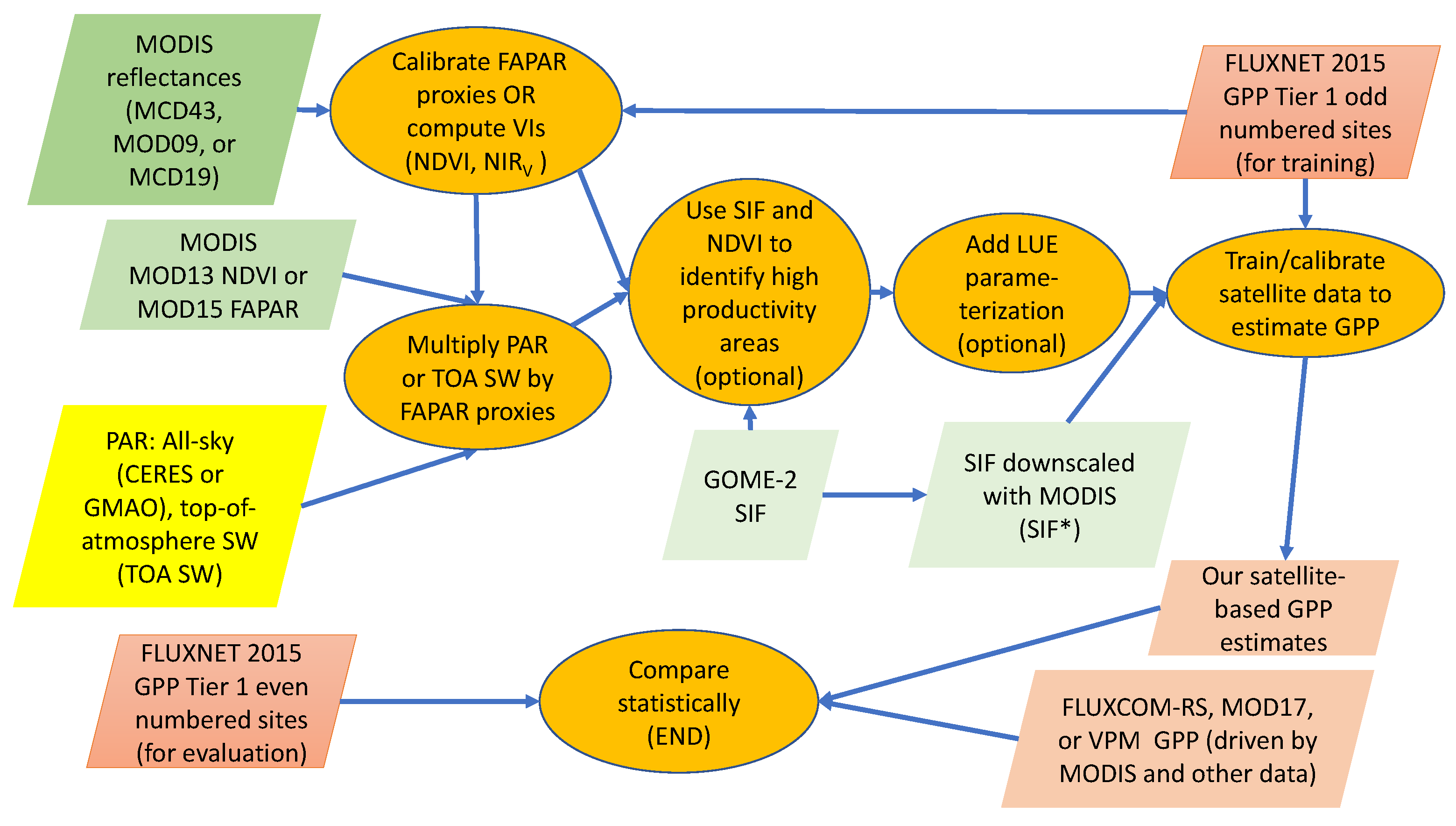
Using the approach shown in Figure A1, we tested a variety of products and models using GPP derived from a consistent sample of eddy covariance sites to both train GPP satellite-driven models and evaluate them. A particular satellite data-driven model is given by GPP $=bx$, where a model parameter x, such as NDVI × SW${}_{\mathrm{TOA}}$, is used to predict flux tower estimates of GPP and b is determined by fitting to a subset of flux tower data.

We investigated the impact of using different MODIS datasets in Appendix A. Generally, MCD43D provided superior results as compared to most other datasets. Our results in the remainder of this paper focus on the MCD43D reflectances that can be used at their highest resolution (∼1 km) or degraded to be comparable to the resolution of other datasets used for benchmarking.

We also tested the use of different radiation datasets in Appendix C. The use of top-of-atmosphere shortwave (SW${}_{\mathrm{TOA}}$), computed as being proportional to cosine of the solar zenith angle (SZA) integrated over a day, as compared with the satellite-derived all-sky SW produced the best results with Equation (2) where LUE was assumed constant. These results are consistent with those of Gitelson et al. [39] and Peng et al. [40], who used a limited number of flux tower sites. Those studies found that GPP did not follow PAR${}_{\mathrm{in}}$, but rather that other factors affect GPP, and that the use of PAR${}_{\mathrm{pot}}$ reduces some of the variability resulting from the dependence of LUE on cloudiness. This would occur if LUE is not constant, but rather anti-correlated with PAR${}_{\mathrm{in}}$ (or correlated with cloudiness), such that various combinations of PAR${}_{\mathrm{in}}$ and LUE produce a relatively constant GPP over a range of cloud conditions and for a given fixed value of FAPAR${}_{\mathrm{chl}}$. It is well known that LUE is higher in situations with more diffuse light (e.g., [36]) (i.e., cloudy conditions) as compared with clear-sky conditions. One exception is very low light conditions where LUE saturates.

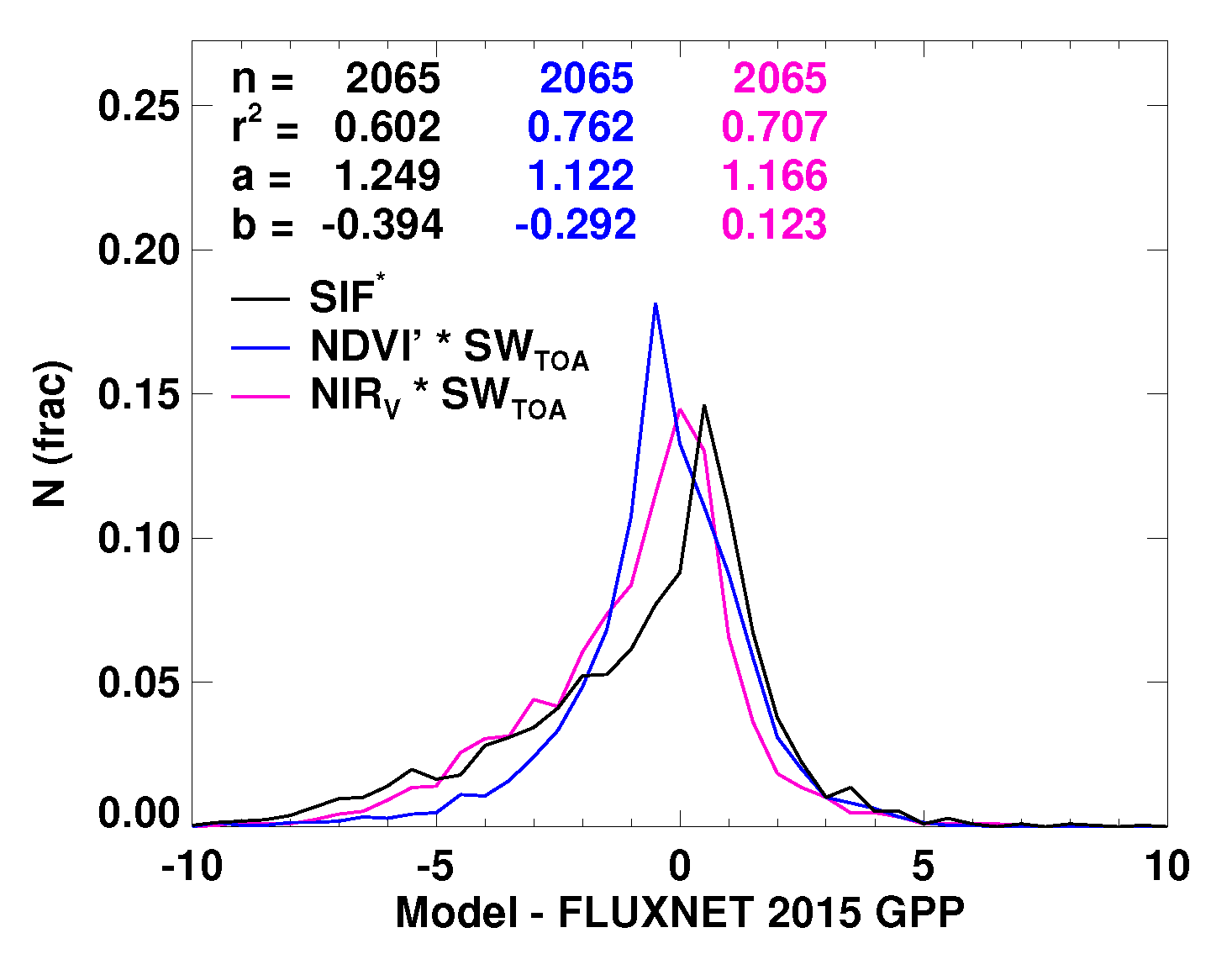
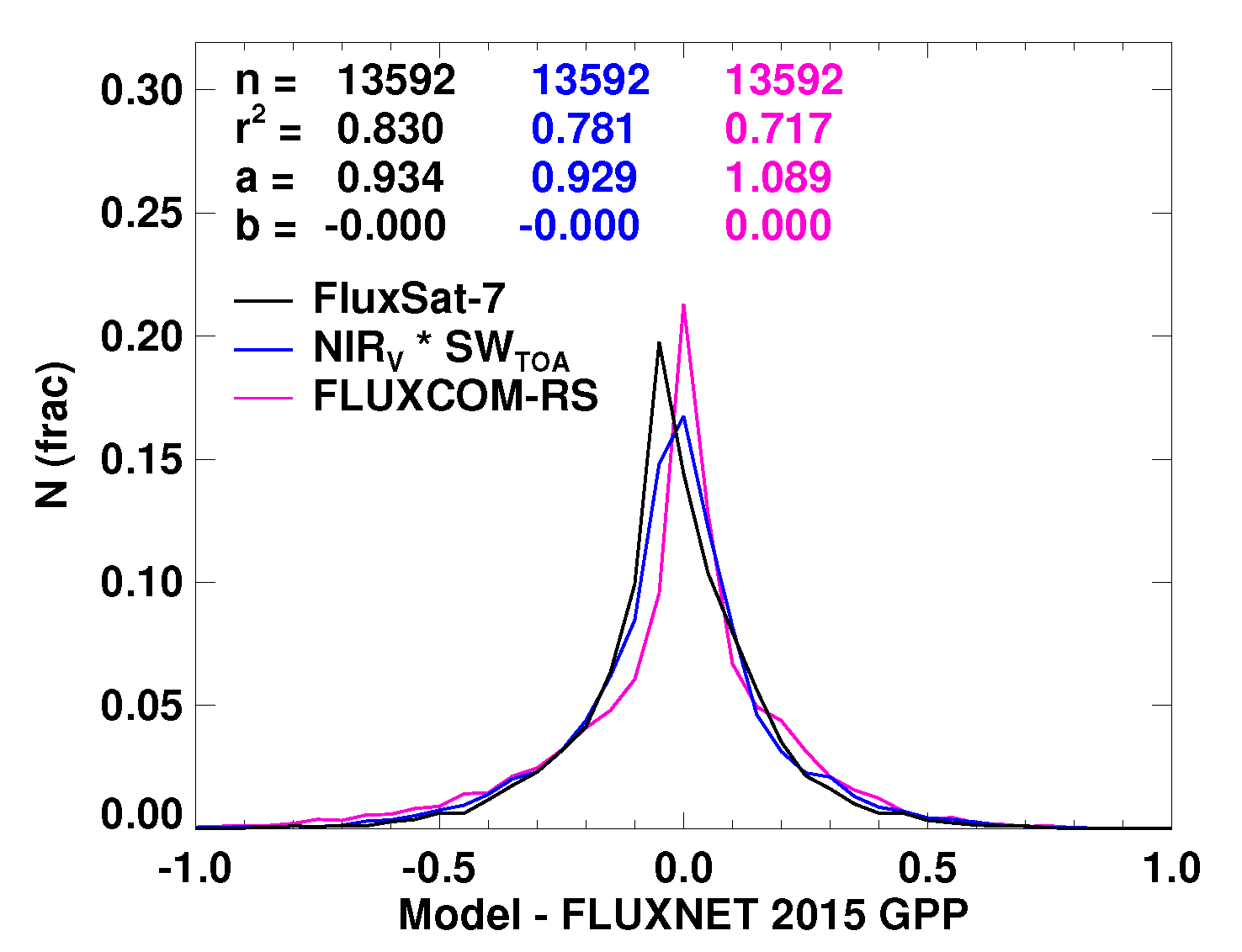
For following comparisons between models and flux tower data, results are typically shown in terms of scatter diagrams or 2D histograms with accompanying statistics. For completeness, we also provide probability distribution functions in Appendix D. These show the degree to which the differences follow a normal distribution that is assumed in statistical significance tests. While the differences deviated somewhat from normal distributions, the number of samples was large enough in most cases that the significance tests (when p-values were very small) were assumed to be valid.

3.1. The Use of Downscaled SIF to Estimate GPP

Duveiller and Cescatti [67] showed that SIF* agreed better with flux tower GPP as compared with MOD17 GPP (see Appendix A for a description of MOD17). Here, we further evaluate SIF* by comparing it consistently with the results of our models. We first verified that all of our models also outperformed MOD17 GPP on eight-day to monthly time scales in all statistical measures. Note that because SIF depends upon incident radiation, we did not explicitly use PAR in SIF-based models (other than to normalize it appropriately as described above); here, we simply applied a single scaling factor to SIF* at monthly time-scales to estimate GPP globally. The assumption of a single scaling factor to relate SIF to GPP, at least encompassing many plant functional types, has been suggested [53,74]; however, the use of a single scaling factor was not generally supported by previous studies (e.g., [46]).

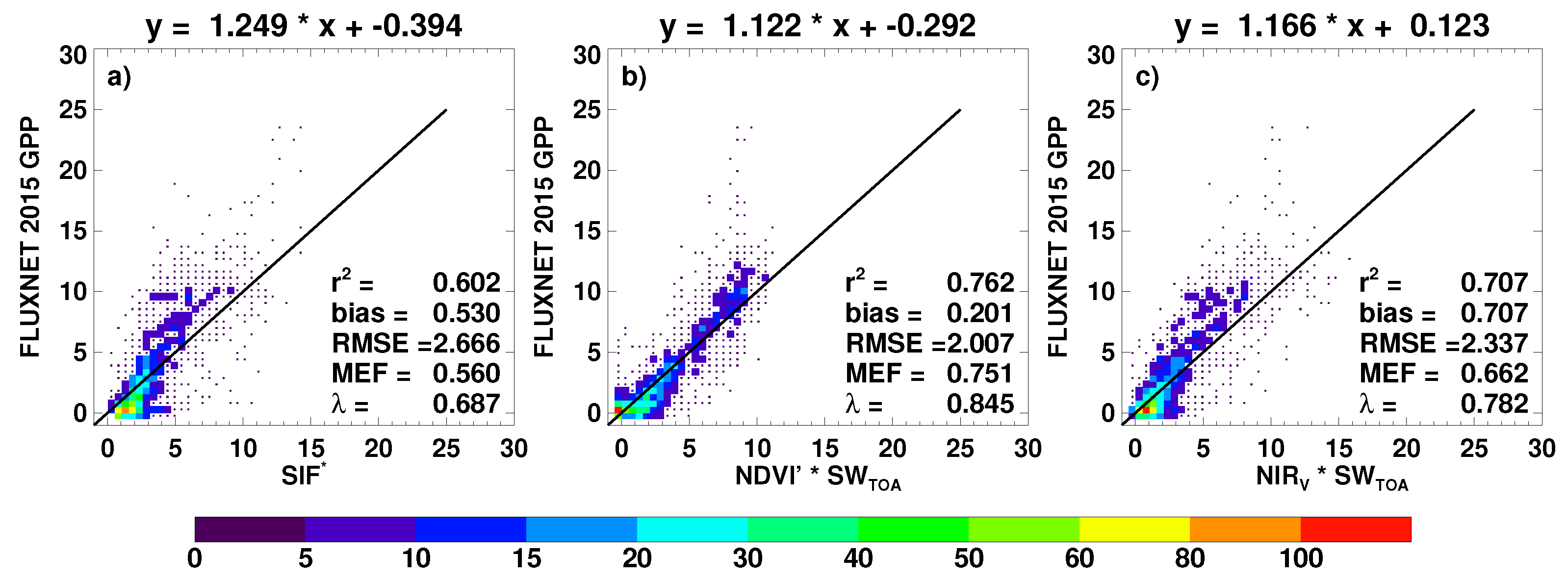
We examine monthly SIF* along with NDVI${}^{\prime }$ and NIR${}_V$ results in more detail in Figure 3 by comparison with tower-derived GPP for years 2007–2013 when GOME-2 SIF v25 data were available. Note that the resolution for SIF* was 0.05${}^{\circ }$, while the MCD43D reflectances had been resampled to 0.083${}^{\circ }$; note that the MCD43D results were degraded as compared with the ∼1 km${}^2$ results in

Table A5. Statistical comparison between various monthly-averaged GPP estimates from MCD43D reflectances (0.00833${}^{\circ }$ resolution) at 64 unique independent flux tower sites from FLUXNET 2015 (models were trained using data from 64 other sites) with a total of 3702 individual collocated observations including the variance explained ($r^2$), bias (mean of flux tower GPP minus the satellite-derived GPP), root mean squared error (RMSE) of the model, model efficiency factor (MEF) (Equation (9)) and $\lambda$ (Equation (10)); units for bias and RMSE are g C m${}^{-2}$ d${}^{-1}$; all others are unitless.

Model Predictor x	${\mathit{r}}^2$	Bias	RMSE	MEF	$\mathit{\lambda }$
NIR${}_V$	0.692	−0.347	2.17	0.679	0.799
NIR${}_V$ × SW${}_{\mathrm{CERES}}$	0.696	0.194	2.12	0.692	0.811
NIR${}_V$ × SW${}_{\mathrm{TOA}}$	0.776	0.045	1.82	0.775	0.878
NDVI × SW${}_{\mathrm{CERES}}$	0.554	−0.145	2.58	0.544	0.681
NDVI × SW${}_{\mathrm{TOA}}$	0.773	−0.389	1.94	0.744	0.837
NDVI${}^{\prime }$ × SW${}_{\mathrm{TOA}}$	0.776	−0.167	1.78	0.783	0.875

, which were much closer to the footprint of the eddy covariance technique [34]. While the positive SIF* bias was clearly seen at GPP values near zero, SIF* was shown to have a more dynamic range as compared with the NDVI${}^{\prime }$-based GPP estimates; NDVI${}^{\prime }$-based GPP estimates tended to saturate at around 10 g C m${}^{-2}$ d${}^{-1}$; while SIF* and NIR${}_V$-based estimates reached values close to 15 g C m${}^{-2}$ d${}^{-1}$. SIF* appeared somewhat noisier than the NDVI${}^{\prime }$- or NIR${}_V$-based GPP estimates. This was expected as the downscaled SIF was directly tied to the more coarsely-gridded GOME-2 SIF that was inherently noisy due to the very small SIF signal. Correlations were significantly different between all three models (i.e., null hypothesis rejected) with p-values $<0.0001$.

The apparent noise in SIF* may also have resulted from the effects of vegetation structure on the escape of SIF through the canopy [75,76]. We attempted to account for the variations in canopy escape as suggested by Yang and van der Tol [76] using MODIS Band 2 (near infrared) reflectance for normalization. However, we did not find improvement in the global statistics. One explanation is that the approach may not work well when bare soil contributes significantly to the observed reflectance and/or because the wavelengths of the MODIS reflectances are not optimal for this purpose.

While the SIF* results were noisy as compared with reflectance-based approaches, we were encouraged by these initial SIF* results given that only a single scaling factor was applied. We expect improvements in subsequent versions of SIF* that will use more recent datasets for SIF, as well as the high spatial resolution variables employed for downscaling. In addition, we expect progress to be made in developing methods to account for the effects of vegetation structure on SIF escape from the canopy globally.

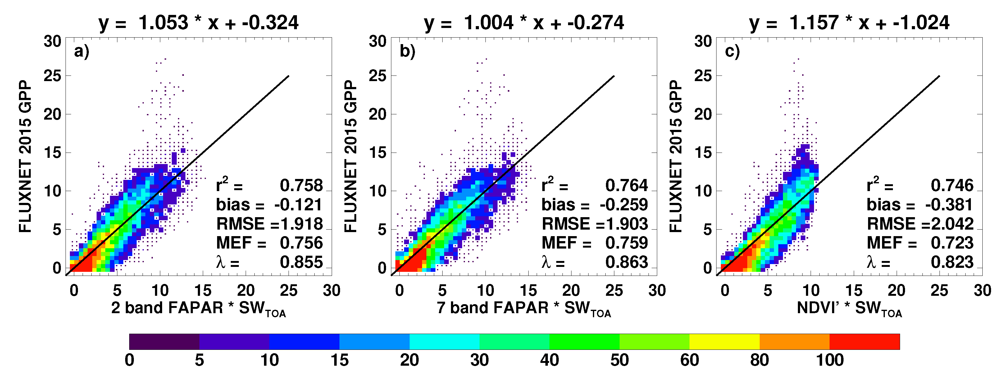
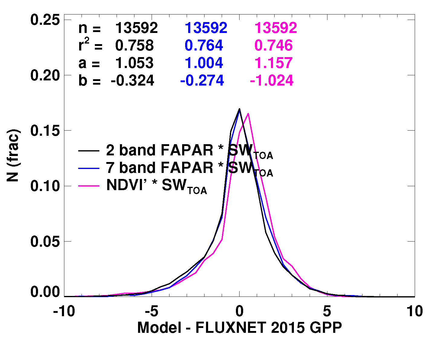
3.2. Use of Linear Combinations of Bands Rather Than VIs

Figure 4 shows results at an eight-day temporal resolution and the highest spatial resolution used here (0.0083${}^{\circ }$) for two- and seven-band models where linear combinations of bands were used as FAPAR${}_{\mathrm{chl}}$ proxies according to Equation 7. Both band models provided improved dynamic range in estimated GPP as compared with the NDVI${}^{\prime }$-based model, and the correlation improvements were statistically significant with p-values < 0.025. The seven-band and two-band models were not statistically distinguishable. All models underestimated GPP at the highest GPP values.

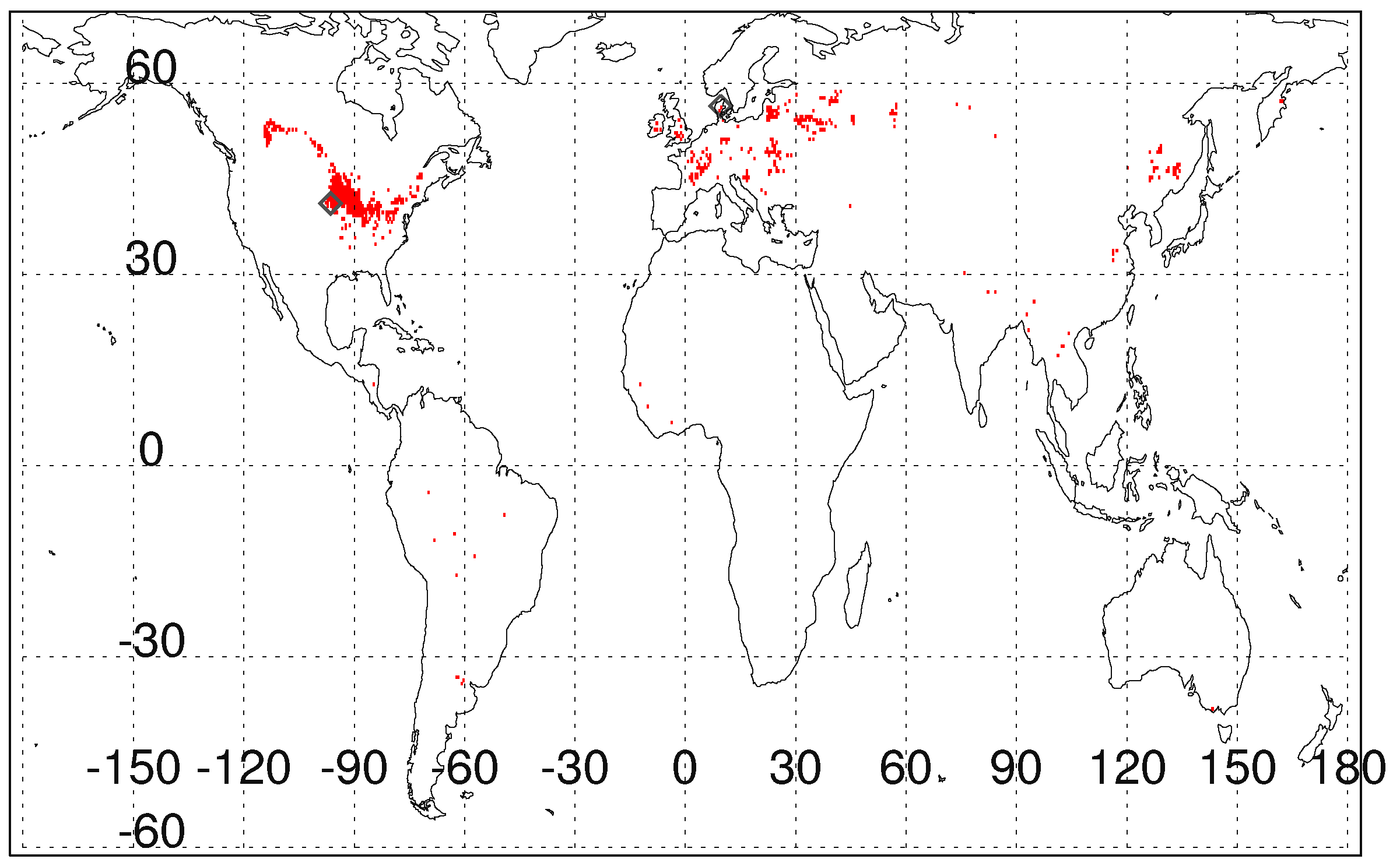
3.3. Use of SIF to Delineate Highly Productive Agricultural Areas

One vegetation type for which GPP was not well predicted by our global linear regression models is croplands with GPP $>\sim$15 (see Figure 3b and Figure 4). An examination of these points shows that they are primarily from three sites in the U.S. Corn Belt (US-Ne1, US-Ne-2 and US-Ne3) that are frequently planted with maize, a C4 plant. Zhang et al. [21] used various datasets to compute grid box fractions of C4 plants (natural and agricultural) for the VPM and defined different maximum efficiencies for C3 and C4 plants within their LUE formulation. The datasets used to compute C4 fractions were static (i.e., no interannual variability) and at lower spatial resolution than the VPM datasets.

Here, we explore an alternative approach that uses satellite-based SIF to delineate highly productive regions. Guanter et al. [32] demonstrated that SIF was more highly correlated with GPP than EVI at flux tower sites located in the U.S. Corn Belt because EVI, like NDVI, displays saturation at high values. They also showed that data-driven models, such as the predecessors of FLUXCOM-RS, did not produce the very high values of GPP derived from flux towers in this region. Global maps of SIF show very high values in summer in these same regions, while NDVI and EVI do not [32]. Here, we test the use of SIF observations, albeit at low spatial resolution (0.5${}^{\circ }$), to identify these regions of high productivity not prominent in the NDVI that may be related to large fractions of highly productive crops that are not well captured by the reflectances alone.

Using collocated GPP, SIF and NDVI data, we found that the FLUXNET 2015 sites with high maximum GPP values that were not well fit using our single linear regression models displayed the following criteria of high NDVI and a large ratio of SIF to NDVI when normalized appropriately by PAR: specifically, NDVI${}_t>$ 0.76 and SIF${}_t$/(NDVI${}_t\times cos\left(\theta \right))>$ 3.0, where t is the month with the highest climatological value of NDVI and $\theta$ is the average solar zenith angle for that month corresponding to the GOME-2 SIF observations. The climatological monthly means are computed over the years 2007–2016. Figure 5 shows a map of the areas detected with this approach. Adjusting the thresholds upwards resulted in somewhat less flagging over areas outside the U.S. Corn Belt (e.g., Eurasia) and vice versa. Additional flux tower sites in high productivity agricultural regions may help to further constrain the thresholds.

To improve GPP estimates with the simple linear regression approaches, we separated the flux tower data into two different samples, one meeting the above criteria for high GPP and SIF and the other not. We then performed separate linear fits to the GPP data for these two subsets. The designated high productivity sites included in the training set were US-Ne1, US-Ne3 and DK-Fou, and the only site in the validation dataset was US-Ne2.

Table 2. Statistical comparison between daily-averaged GPP estimates using MCD43D data at 0.00833${}^{\circ }$ resolution from satellite data at 64 independent unique flux tower sites from FLUXNET 2015 with a total of 10,3671 individual collocated observations.

GPP Estimate	${\mathit{r}}^2$	Bias	RMSE	MEF	$\mathit{\lambda }$
NIR${}_V$ × SW${}_{\mathrm{TOA}}$	0.694	0.018	2.19	0.695	0.824
NDVI${}^{\prime }$ × SW${}_{\mathrm{TOA}}$	0.693	−0.306	2.21	0.691	0.806
NDVI${}_2^{\prime }$ × SW${}_{\mathrm{TOA}}$	0.718	−0.249	2.16	0.707	0.814
7band × SW${}_{\mathrm{TOA}}$	0.700	−0.262	2.20	0.696	0.818
7band${}_2$ × SW${}_{\mathrm{TOA}}$	0.725	−0.238	2.11	0.720	0.831

shows the results of the validation from this dual fit approach, henceforth referred to as NDVI${}_2^{\prime }$ or 7band${}_2$. The statistics shown here are for daily data. We note significant improvement in metrics with flux tower GPP with dual fit as compared with the single fit models (null hypothesis rejected). These results demonstrate a clear capability of the satellite data to estimate GPP down to a daily time scale. Note that for the band models, the coefficients for each band in the calculation of FAPAR${}_{\mathrm{chl}}$ proxies in Equation (7) were estimated using all flux tower training data. Only the slopes between GPP and the product of FAPAR and PAR proxies were computed using the two different samples.

Even though the results using SIF were positive, there is room for improvement. The use of a low-resolution static SIF dataset has obvious limitations. We do not account for the fact that only a fraction of our identified high productivity grid boxes was covered by highly productive crops. Improved SIF datasets are expected in the near future that will address some of these concerns as explained below.

3.4. Further Parameterization of LUE

Bauerle et al. [77] found that photoperiod explained more seasonal variation in leaf photosynthetic capacity (related to LUE) than temperature. Zhang et al. [78] also derived a seasonally-varying photosynthetic capacity from satellite SIF and other measurements and showed that using this seasonal variation within a canopy transport model improved estimates of GPP and LUE. Functions of NDVI have been used to account for these seasonal variations in LUE [29,30].

We tested various expressions of seasonal variation of LUE in an attempt to further improve our satellite-based GPP estimates. We found that a small portion of the remaining variance in LUE can best be modeled as a simple polynomial expression of NDVI. In this model, we have for each of the two separate fits within the dual fit approach,

$$\mathrm{GPP}={\mathrm{FAPAR}}^{\prime }\times {\mathrm{SW}}_{\mathrm{TOA}}\times (a+b\mathrm{NDVI}+c{\mathrm{NDVI}}^2),$$

(11)

where FAPAR${}^{\prime }$ is an FAPAR proxy such as NDVI${}^{\prime }$ or multi-band proxies. Other LUE parameterizations tested included second order polynomials in SW${}_{\mathrm{TOA}}$, SW${}_{\mathrm{TOA}}/$max(SW${}_{\mathrm{TOA}}$), or NDVI/max(NDVI) for each location as proxies for photoperiod or products of these predictors. However, the straight NDVI parameterization provided the best results.

Figure 6 shows results for our dual fit seven-band variable LUE (Equation (11)) models that we will refer to as FluxSat-7, the dual fit NDVI${}^{\prime }$-based variable LUE model (FluxSat-N), as well as NIR${}_V$-based results at eight-day temporal resolution. At the 0.00833${}^{\circ }$ spatial resolution of MCD43D, both FluxSat-7 and FluxSat-N were more centered about the 1:1 line than the NIR${}_V$-based model, and correlation differences between FluxSat and the NIR${}_V$-based models were statistically significant with very low p-values. The FluxSat-7 correlation improvement over FluxSat-N was significant with a p-value of 0.05. Improvements were obtained with the NDVI-dependent LUE as compared with the results in Figure 4.

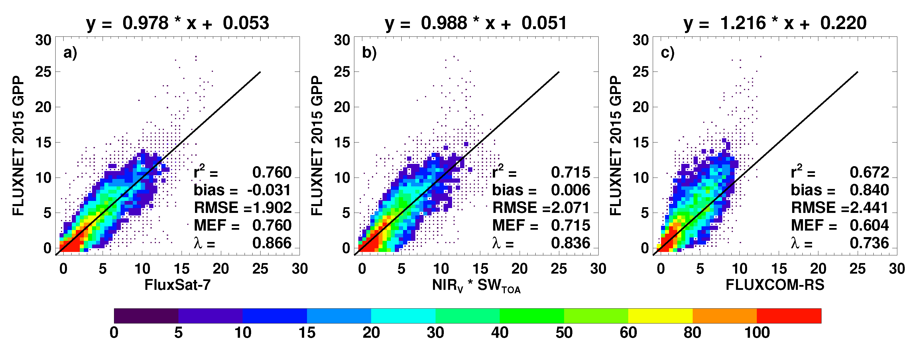
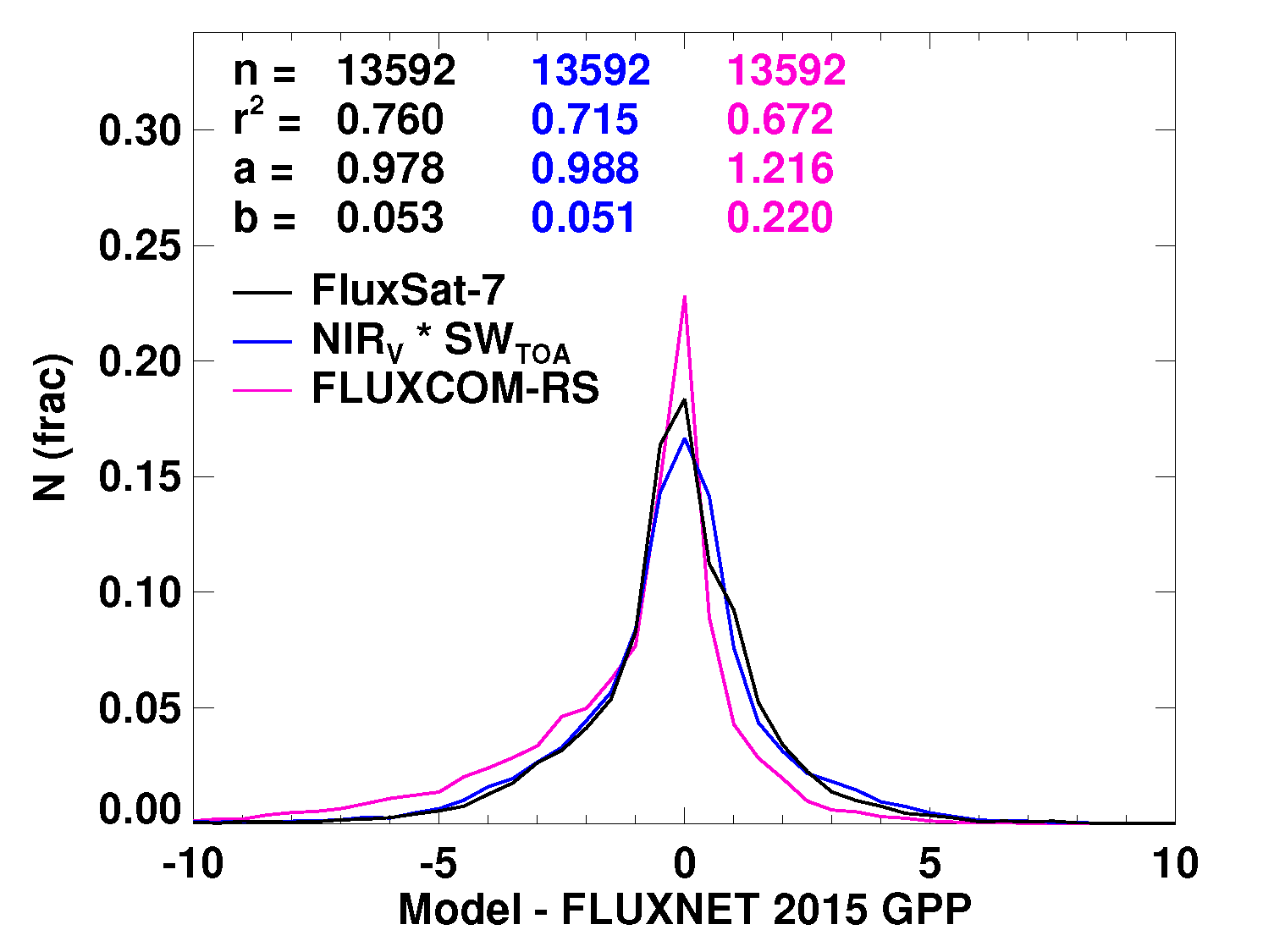
3.5. Comparison with Other Satellite Data-Driven GPP Estimates

Next, we compare FluxSat-7 and NIR${}_V$-based GPP with that from state-of-the-art data-driven FLUXCOM-RS and VPM. Figure 7 shows 2D histograms of FluxSat-7, NIR${}_V$-based and FLUXCOM-RS eight-day GPP estimates at 0.0833${}^{\circ }$ resolution versus independent FLUXNET 2015 data. At this spatial resolution, all three generally overestimated GPP at low values and underestimated at high values. FluxSat-7 had the best performance at the highest values of FLUXNET 2015 GPP. All correlations were statistically different (p-values < 0.0001). FluxSat-7 showed the highest overall correlations with respect to FLUXCOM 2015. As shown above, comparisons with FLUXCOM 2015 at the full spatial resolution of MCD43D (0.0083${}^{\circ }$, Figure 6) provided superior results as compared with results at the spatial resolution of FLUXCOM-RS (0.083${}^{\circ }$).

We note that FLUXCOM-RS was not trained with FLUXNET 2015 data, but rather with a different processing of an overlapping subset of eddy covariance flux tower data from the La Thuile dataset [10]. This may explain the bias of FLUXCOM-RS with respect to FLUXNET 2015 that was not present with respect to the La Thuile training dataset [10]. The bias may be easily removed using a linear regression with respect to FLUXNET 2015. When this was done, we obtained statistics that were similar to the single fit models presented in Section 3.2 applied at the same spatial resolution; the highest GPP values from the US-Ne3 site were still not well matched with FLUXCOM-RS after this adjustment.

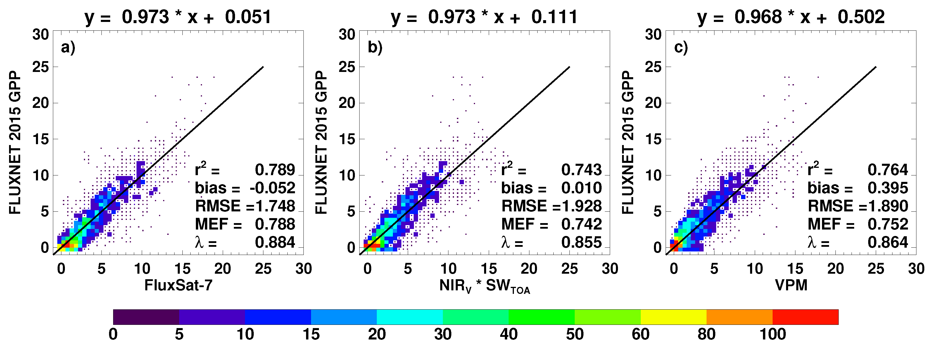
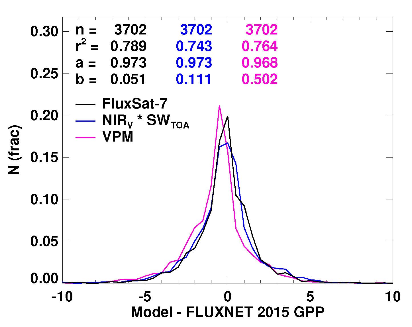
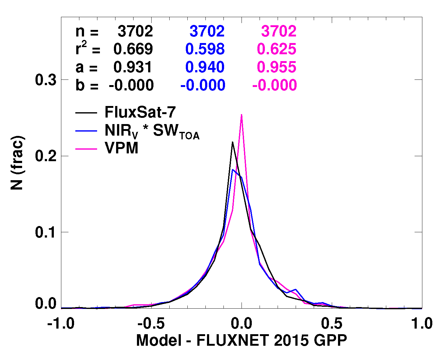
Figure 8 similarly shows 2D histograms for monthly GPP averages for VPM, FluxSat-7 and NIR${}_V$-based versus FLUXNET 2015. Again, all models reproduced the tower-based GPP estimates reasonably well. As expected, results were improved as compared with those at lower spatial and higher temporal resolution in Figure 7. FluxSat-7 showed a somewhat lower spread and a bit less underestimation at high GPP values with statistically-significant improvements in correlations over the other two models.

3.6. Comparison of Interannual Variations (IAVs)

Figure 9 and Figure 10 show 2D histograms similar to Figure 7 and Figure 8, but this time of normalized GPP differences from the climatology (also known as anomalies or IAVs). To compute the normalized IAVs, the seasonal cycle of GPP was first removed, then the remaining differences were normalized by the range of observed climatological values from the FLUXNET 2015 data for each individual location (known as the min-max normalization). For example, a normalized value of 0.5 means that a positive difference is 50% of the range of observed GPP. If the min-max normalization was not performed, then analyses suggested that the models did not capture IAVs well.

All models were able to reproduce GPP IAVs well. FluxSat-7 provided improved results as compared with the other models. This was the case particularly for the points with the largest IAVs (both positive and negative). All correlations were different with high statistical significance.

3.7. Comparison of Spatio-Temporal Variation in GPP

Figure 11 examines the spatio-temporal variation in annual GPP produced by the different satellite data-driven models. Each point on the scatter diagrams represents a mean annual value for a particular site and year where only the independent sites (i.e., not used in training of either NIR${}_V$ or FluxSat-7) are shown and all datasets are at 0.0833${}^{\circ }$ resolution. Only complete or nearly complete years (i.e., a few missing eight-day segments) are shown, and the same sampling was done for all datasets (i.e., if there was a missing data point for one dataset, it was eliminated for all datasets). The metrics were best for FluxSat-7, but the model differences were not statistically distinguishable in this case.

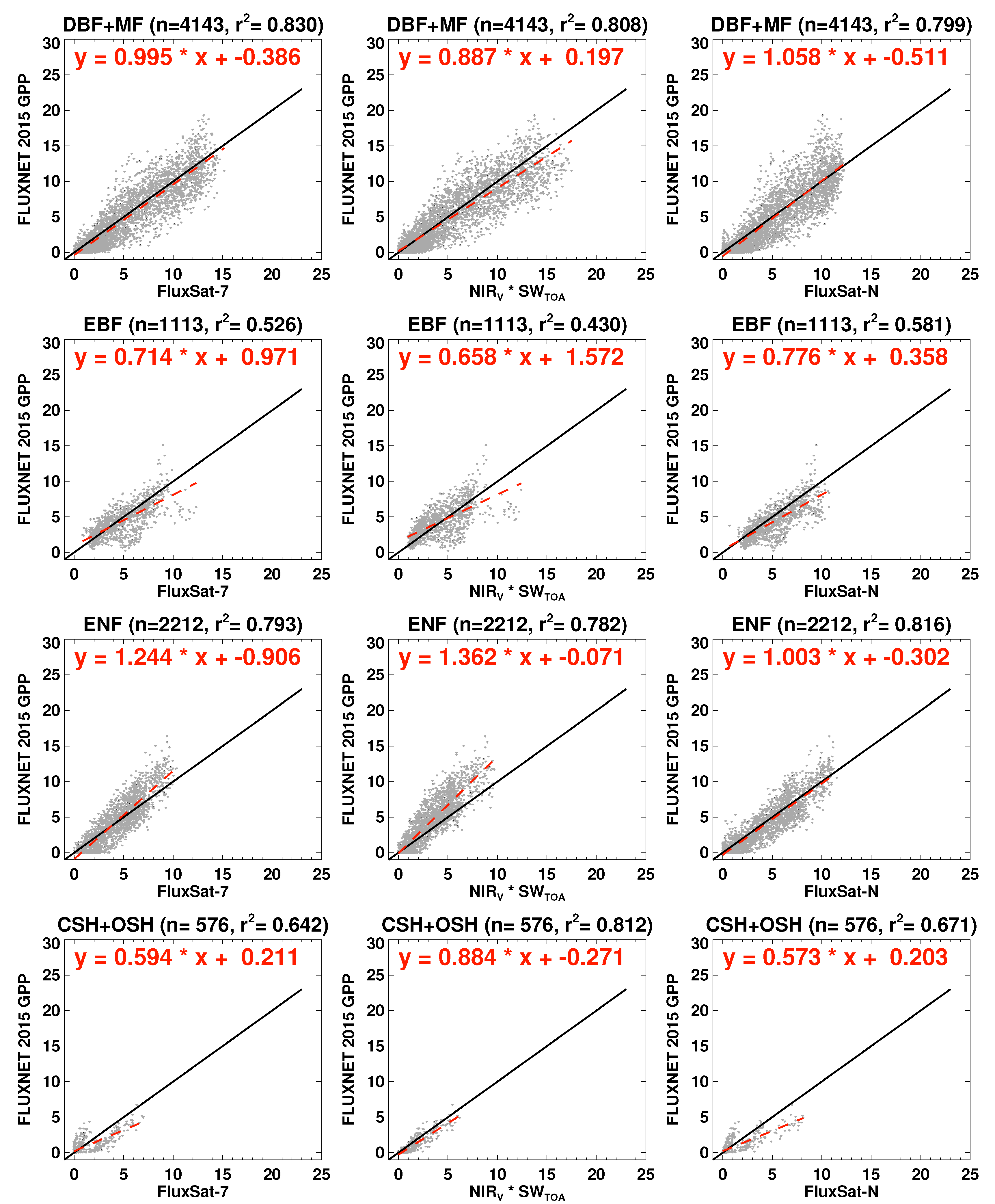
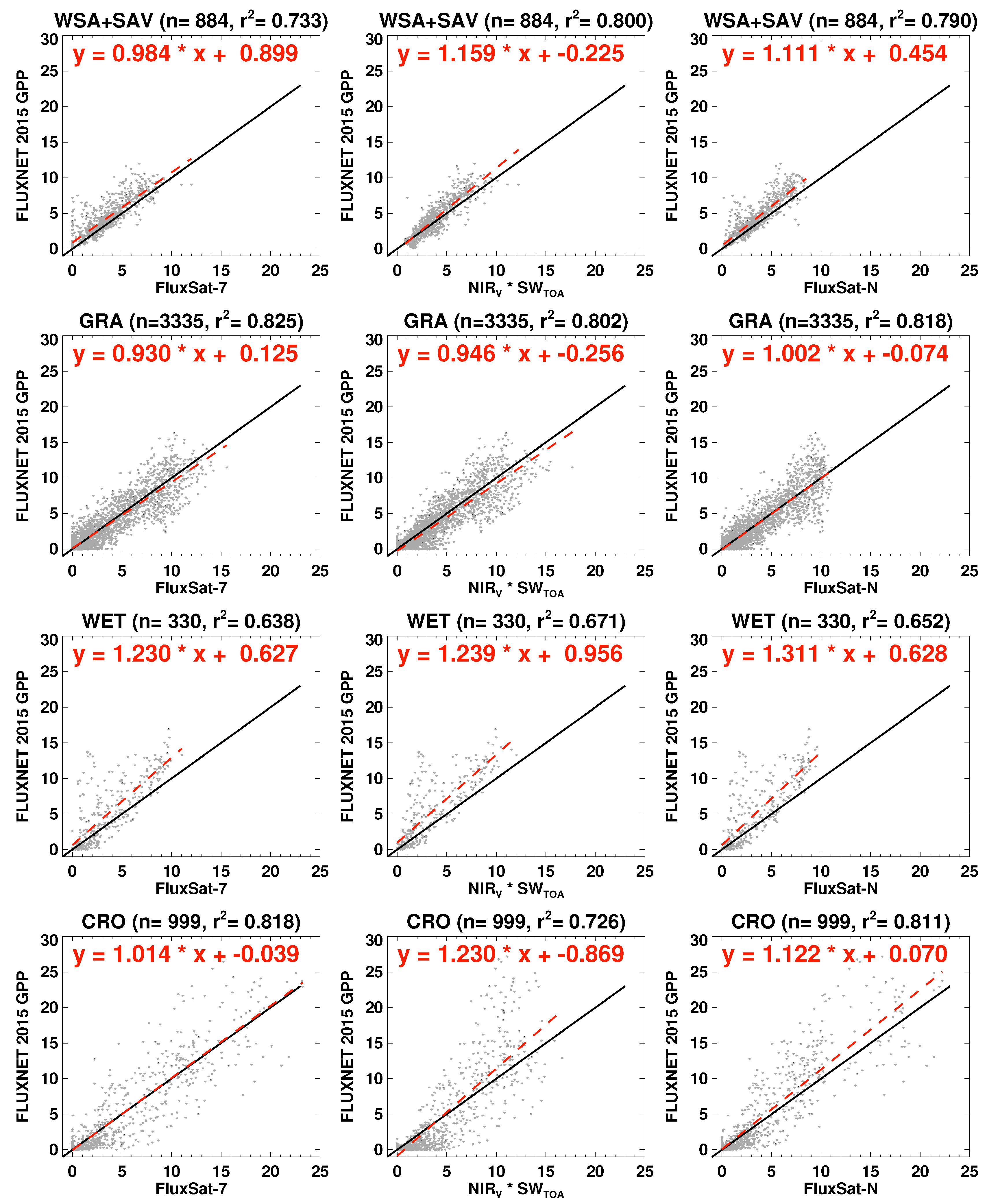
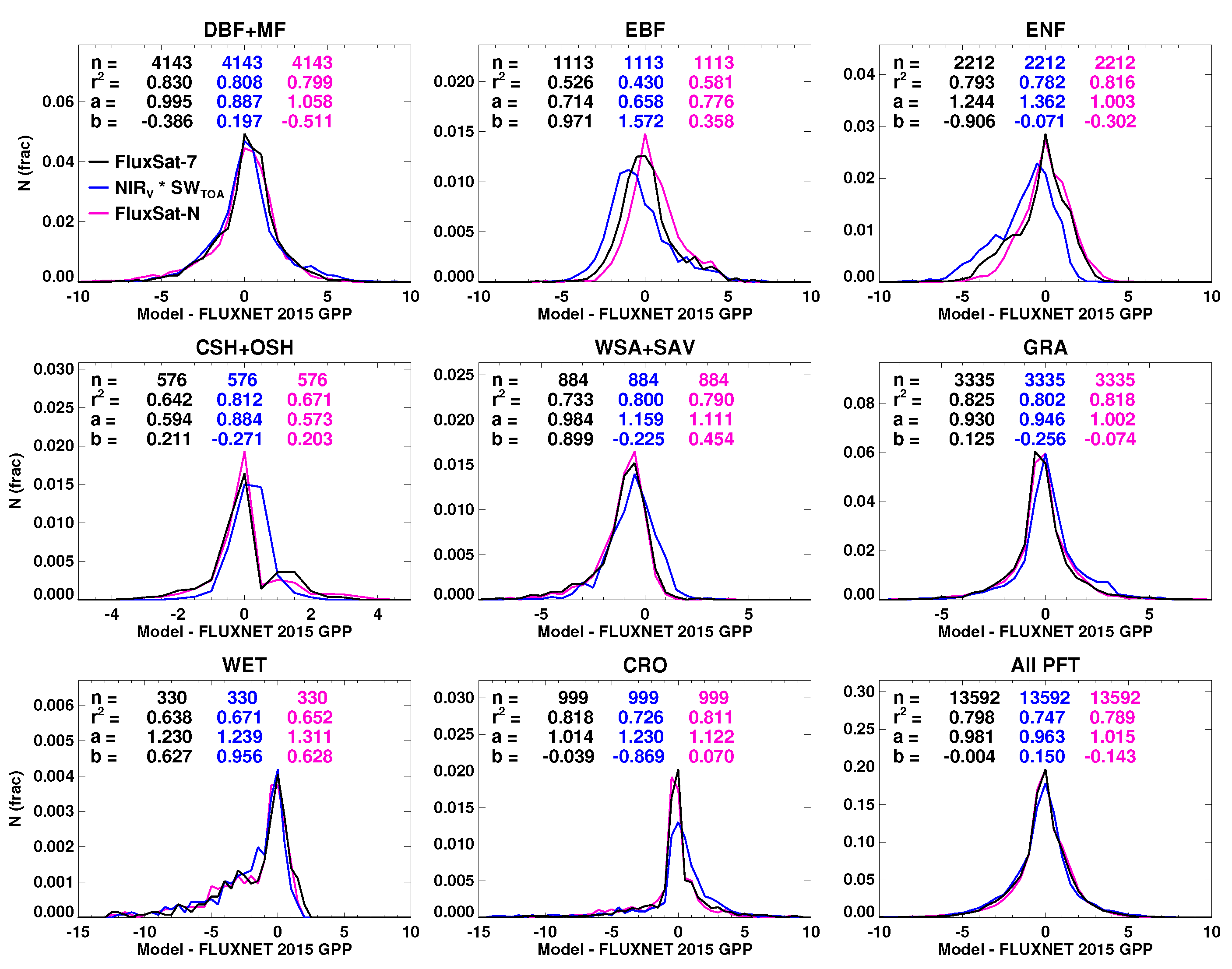
3.8. Comparisons across PFTs

Scatterplots of satellite data-driven GPP estimates (FluxSat-7, NIR${}_V$-based and FluxSat-N at the highest MCD43D resolution of 0.0083${}^{\circ }$ for eight-day data) versus flux-tower estimates are displayed for different PFTs in Figure 12 and Figure 13. All three models showed good performance and relatively low biases across PFTs. On the whole, FluxSat-7 outperformed the other two models with higher correlations and slopes generally closer to unity. NIR${}_V$-based had the most dynamic range for deciduous broadleaf forest (DBF) + mixed forest (MF), followed by FluxSat-7; FluxSat-N showed the smallest range for this type. However, FluxSat-7 and FluxSat-N better reproduced the very high values of GPP found in some cropland sites as shown above.

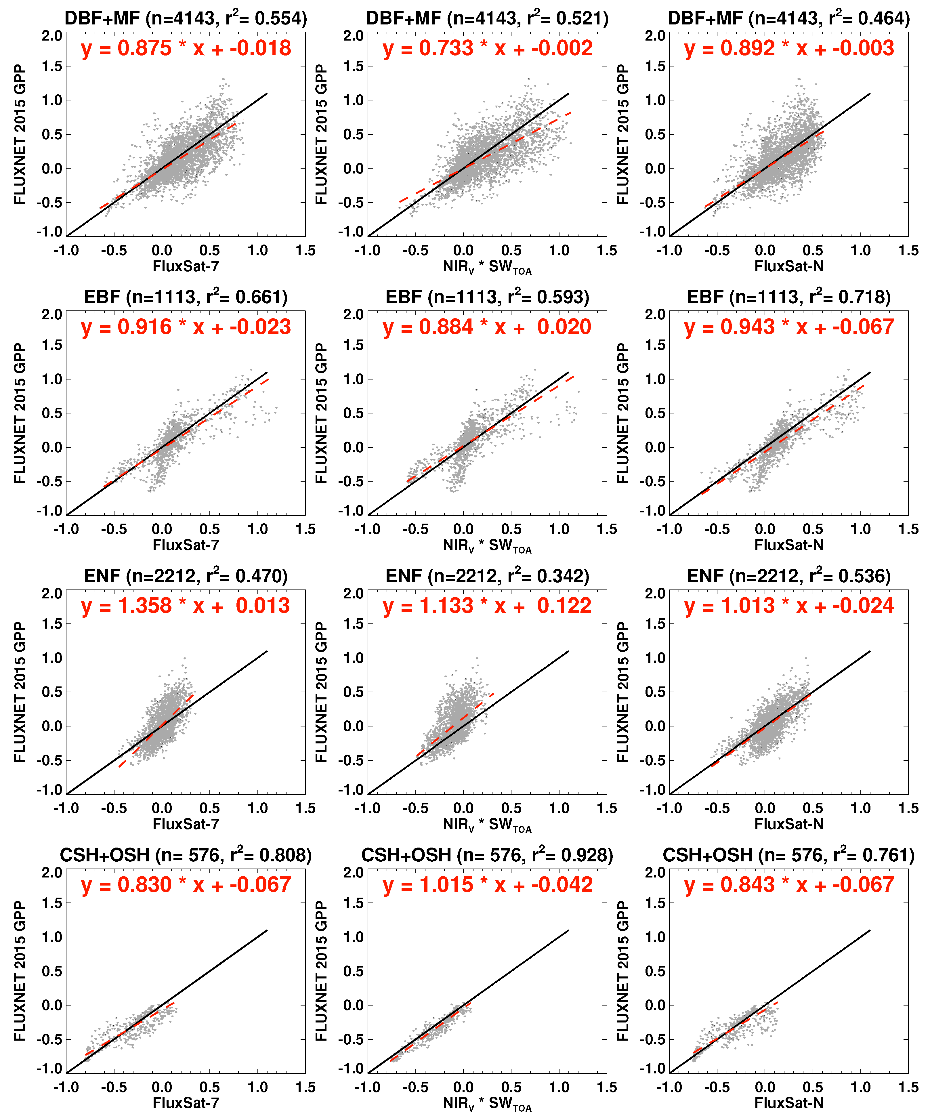
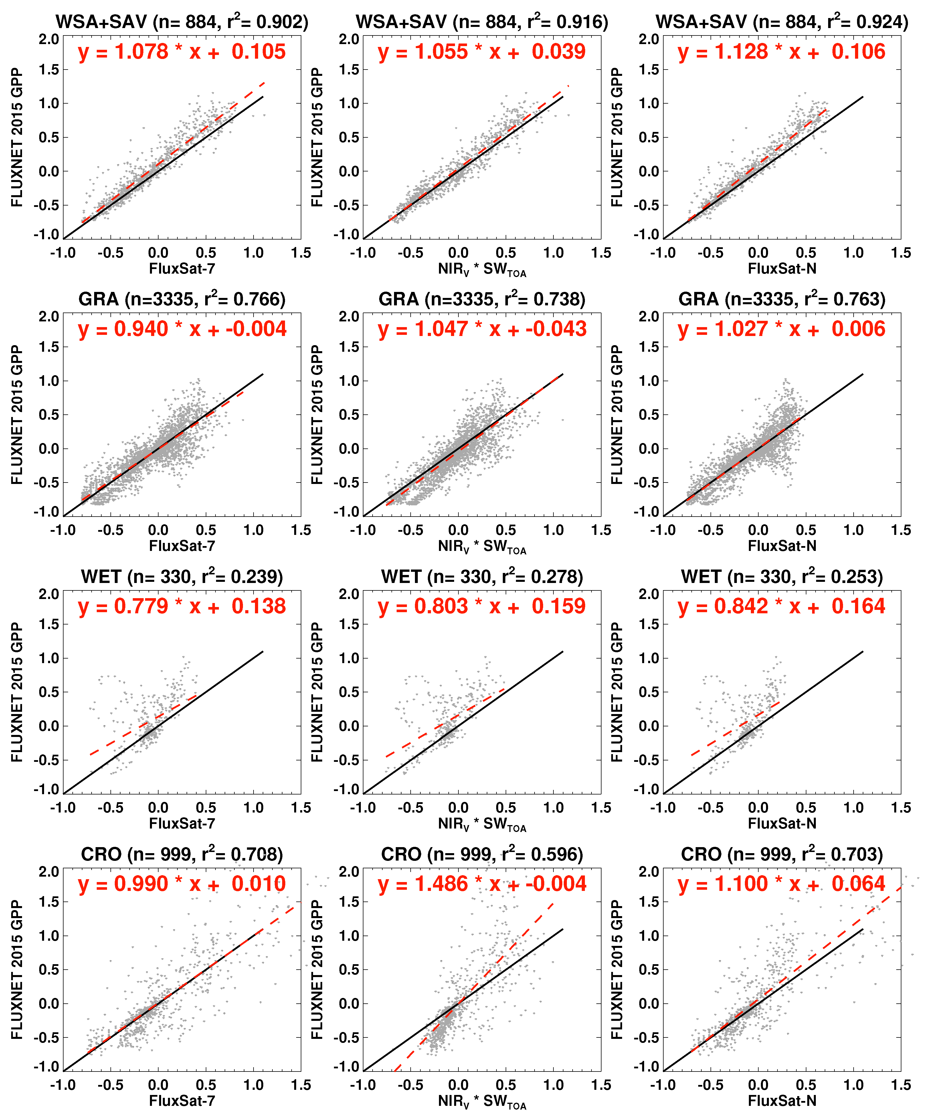
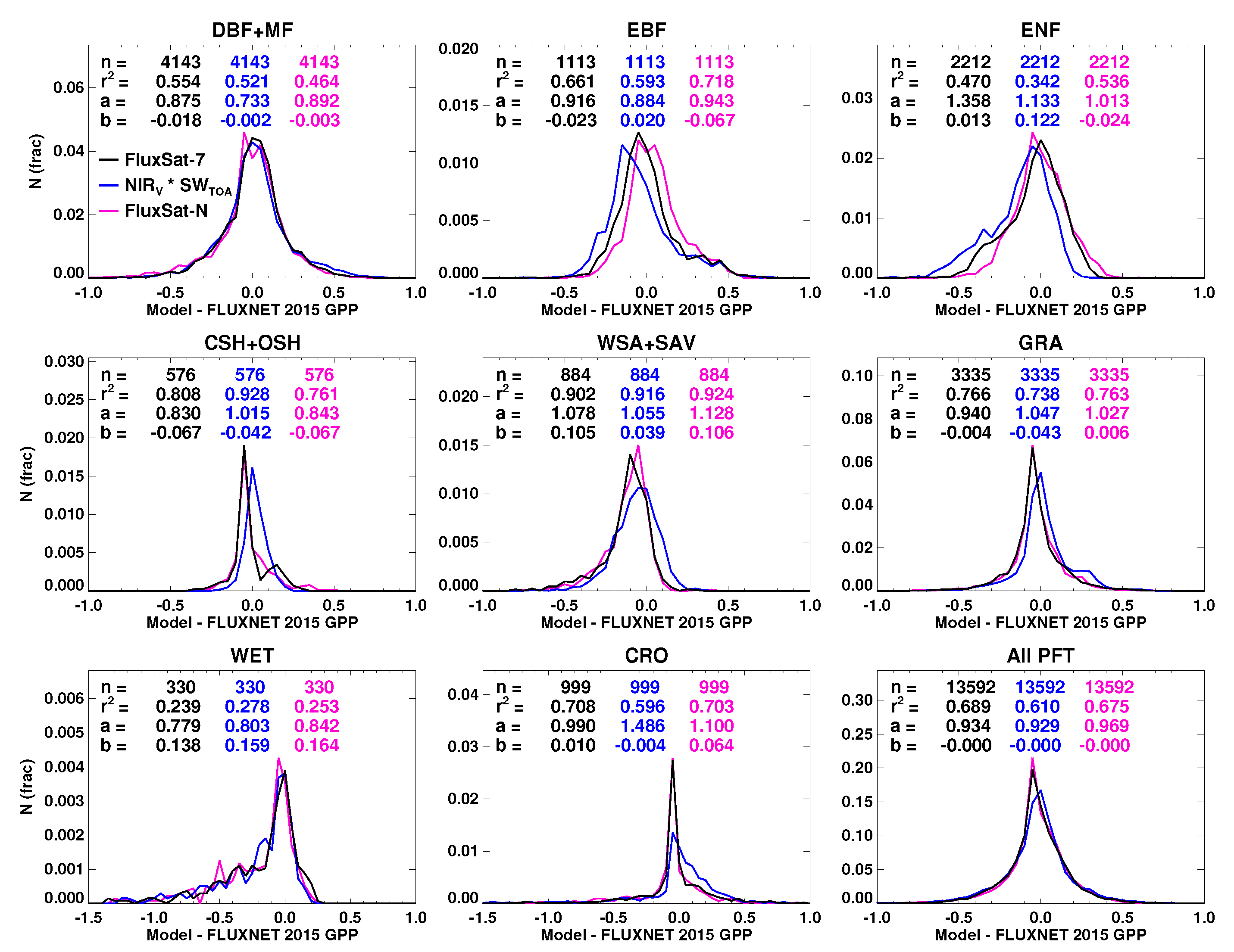
Figure 14 and Figure 15 similarly compare IAVs across PFTs. Again, all three models effectively capture IAVs across PFTs. The models perform particularly well in capturing IAVs for savannas and grasslands. Upon further investigation of the EBF anomalies, we found two distinct clusters of points. The first cluster was for the Australian sites. The anomalies of these sites were well captured by the satellite data-driven models. The second cluster was for two European EBF sites (FR-Pue and IT-Cpz); anomalies from these sites in FLUXNET 2015 were not well captured by our satellite data-driven models.

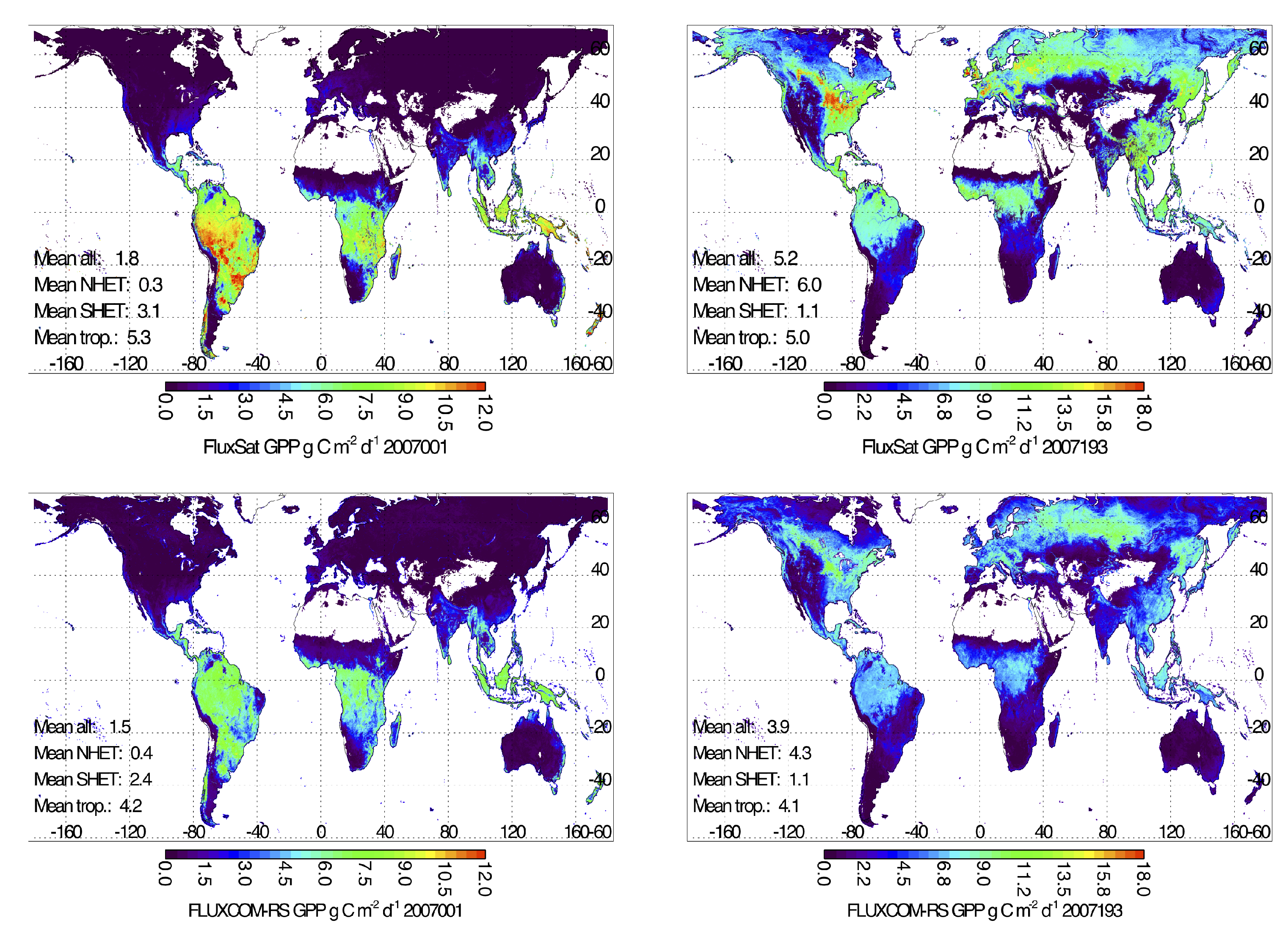
3.9. Comparison of Globally Mapped GPP

Figure 16 shows globally mapped FluxSat-7 and FLUXCOM-RS GPP for two eight-day periods in 2007. As expected based on Guanter et al. [32], large differences are shown in the U.S. Corn Belt and other highly productive agricultural areas identified with the SIF data. GPP values near the peak of the northern hemisphere growing season (for the eight-day period starting at 193) are seen to be generally higher with FluxSat-7 as compared with FLUXCOM-RS; this may be related in part to the different training datasets used. Differences in the winter hemispheres are more similar. FluxSat-7 provided mostly higher values in the tropics as compared with FLUXCOM-RS.

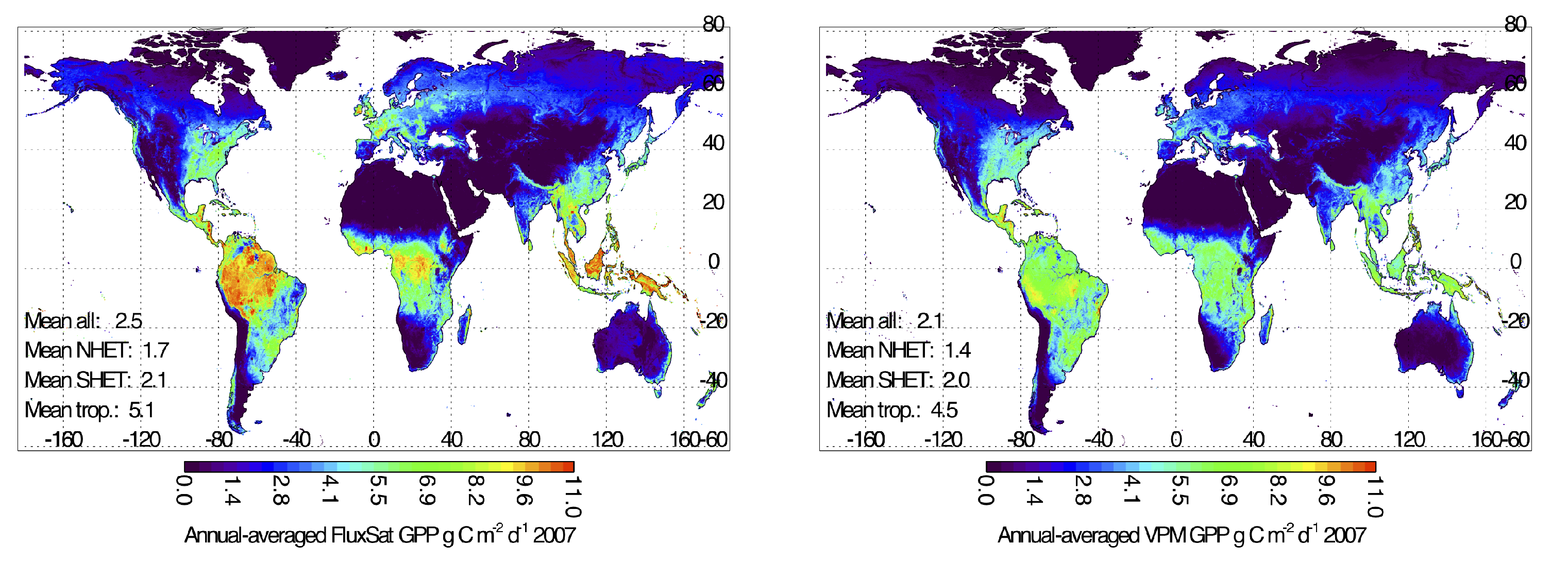
Figure 17 shows maps of annual averaged GPP from FluxSat-7 and VPM. The average values in the Southern Hemisphere extra tropics were similar. However, mean values in both the tropics and Northern Hemisphere extra tropics were higher in FluxSat-7.

To check our results in the tropics, we ran an experiment where half the sites were used for training, but the one tropical station with high GPP values from FluxSat-7, BR-Sa3, was withheld from the training set and was instead used for evaluation. Figure 18a shows that the high GPP values for this site produced by FluxSat-7 were supported by the flux tower values. This is an important finding because this region is frequently cloudy and satellite-derived GPP values have large uncertainties owing to few ground-based training sites.

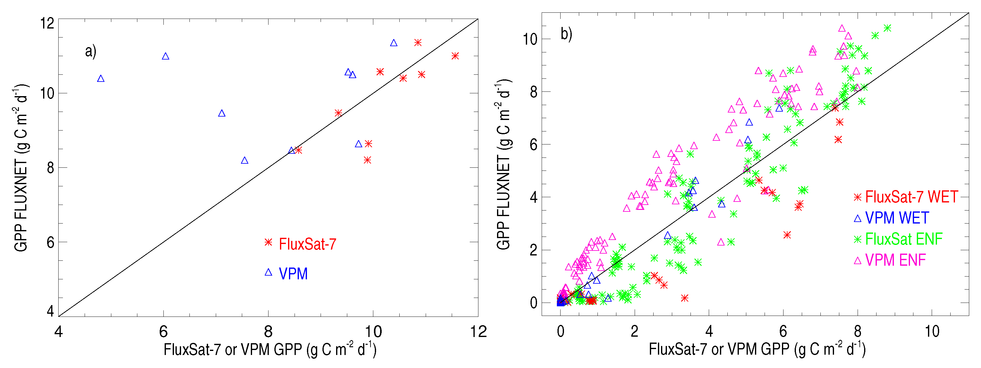
We similarly compare GPP values at four independent high latitude sites (above 60${}^{\circ }$N) in Figure 18b where two sites were ENF and two were wetland. We see that both FluxSat-7 and VPM underestimated GPP at the higher values for ENF sites, while FluxSat-7 somewhat overestimated for wetland sites and lower GPP values at ENF sites. VPM had a more consistent underestimation

The annual GPP values from FluxSat-7, VPM and FLUXCOM-RS were 140.8, 125.0 (in agreement with that reported by Zhang et al. [21]) and 111.6 Pg C y${}^{-1}$, respectively for 2007. If SIF was not used for delineation of high productivity areas, and a single fit to the flux tower data was used for all areas, then FluxSat-7 reduced to 139.4 Pg C y${}^{-1}$. It has been noted that VPM has an underestimation for ENF and EBF that is possibly related to higher light use efficiency for diffuse radiation [21]. It is therefore not surprising to see higher values from FluxSat-7 as compared with VPM for those PFTs that occupy a significant fraction of the vegetated land surface.

FluxSat-7 is within the range of a compilation of observation-based, model, and hybrid results [1], but outside the high range of values from previously reported observation-based diagnostic models [79]. Discussing the evaluation of global annual GPP produced by Earth system models with an earlier version of FLUXCOM (that produced a value of 119 ± 6 Pg C y${}^{-1}$), Anav et al. [80] noted that higher estimates of 150–175 and 146 ± 19 Pg C y${}^{-1}$ were reported by Welp et al. [81] and Koffi et al. [82], respectively, though there were large uncertainties associated with those estimates. How our observation-based GPP values are interpreted within the context of the land sink and budget imbalance in global carbon budget estimates that rely upon dynamic global vegetation models [2] will be a topic for future investigation.

4. Conclusions

Here, we have presented a suite of satellite data-driven models based on the LUE concept to estimate GPP globally. The models were trained (or calibrated) using a subset of eddy covariance flux tower data and evaluated using a set of independent flux tower data. The models did not have any explicit dependence upon PFT; they were trained and evaluated with data across all PFTs with the exception of sites with high SIF relative to NDVI that were trained separately and generally coincided with high fractions of C4 maize crops. These areas represent only a few percent of the total land surface. Our best satellite data-driven models outperformed more complex state-of-the-art data-driven models that may or may not also incorporate ancillary information such as meteorological data.

We find that using SW${}_{\mathrm{TOA}}$ (similar to clear-sky SW radiation) with constant or slowly varying (on seasonal time scales) LUE effectively accounts for the dependence of LUE on incident (cloudy-sky) radiation; specifically, light use efficiency increases with cloudiness index or diffuse radiation fraction in such a way as to produce a relatively constant GPP over a wide range of cloud conditions, and our model effectively accounts for this. This may explain why our GPP estimates are higher than other satellite-based estimates, particularly in the cloudy tropics. Our high derived GPP values in the tropics agree well with the one available tropical Tier 1 FLUXNET 2015 site that has high values. Higher values of estimated GPP in the tropics and also in the extra-tropical Northern Hemisphere lead to higher annual estimated values of GPP (140.8 Pg C y${}^{-1}$ for 2007) with our best model. This is higher than other state-of-the-art satellite-based GPP estimates and on the high end of values from both prognostic and diagnostic models.

We applied a relatively simple adjustment to NDVI data to mitigate the NDVI offset. Models that use NDVI or the two NDVI bands have the advantage that they can be applied to satellite data that date back to the early 1980s from the Advanced Very-High Resolution Radiometer (AVHRR) such as from Tucker et al. [24] or to field-scale imagery from Landsat, Sentinel 2 or other commercial satellites. The linear combination of either two or seven bands provides more dynamic range than the NDVI that tends to saturate at high values.

We find that inclusion of an LUE parameterization in terms of a second order polynomial function of NDVI helps to further explain some variability in GPP. This formulation presumably accounts for variations in the maximum carboxylation rate tied to the photoperiod.

For available input VI-related satellite datasets, we find that better results are obtained when using BRDF-adjusted data as compared with non-adjusted data. We obtained improved results using NDVI computed from averaged reflectances or albedos rather than composited “best-value” NDVI data. We also confirm that in general, better statistical comparisons with the flux tower data were achieved when satellite data are used at high spatial resolution similar to the typical footprint of eddy covariance data (∼1 km${}^2$) as compared with (5–8 km)${}^2$. In terms of temporal resolution, the best results were obtained at monthly temporal resolution, as expected. However, results at eight-day or daily resolution were only marginally degraded as compared with monthly averages.

The best results were obtained when our models took advantage of satellite-based SIF data to identify areas of high productivity. These models also outperformed the NIR${}_V$ for estimation of global GPP. The results overall with downscaled SIF were encouraging given that only a single scaling factor was used and considering that the input datasets have since been updated. However, to be further improved, it is likely that variations in fluorescence escape from the canopy and fluorescence yield will have to be better accounted for.

The reflectance-based models were able to take advantage of high fidelity imager reflectance data with low noise and consequently high spatial resolution and frequent revisit. Our results suggest that machine learning or other similar approaches may benefit from the use of these data along with SIF. While our approach of using a static low resolution SIF dataset to detect high productivity areas is not optimal and can be improved, the number of grid boxes with high SIF relative to NDVI was only approximately 2–3% of all land grid boxes, excluding Antarctica. Therefore, small errors due to temporal variability or the fact that only a fraction of those grid boxes may contain high productivity crops are unlikely to have a significant impact on our global annual GPP estimates. The results obtained here may be further improved using higher spatial resolution SIF data ideally taken over several years, such as from the recently launched TROPOspsheric Monitoring Instrument (TROPOMI) with ground footprints ∼7 km × 3.5 km at nadir and complete daily global coverage [65].

References

1. Anav, A.; Friedlingstein, P.; Beer, C.; Ciais, P.; Harper, A.; Jones, C.; Murray-Tortarolo, G.; Papale, D.; Parazoo, N.C.; Peylin, P.; et al. Spatiotemporal patterns of terrestrial gross primary production: A review. Rev. Geophys. 2015, 53, 785–818. [Google Scholar] [CrossRef] [Green Version]
2. Le Quéré, C.; Andrew, R.M.; Friedlingstein, P.; Sitch, S.; Pongratz, J.; Manning, A.C.; Korsbakken, J.I.; Peters, G.P.; Canadell, J.G.; Jackson, R.B.; et al. Global Carbon Budget 2017. Earth Syst. Sci. Data 2018, 10, 405–448. [Google Scholar] [CrossRef] [Green Version]
3. Peters, G.P.; Le Quéré, C.; Andrew, R.M.; Canadell, J.G.; Friedlingstein, P.; Ilyina, T.; Jackson, R.B.; Joos, F.; Korsbakken, J.I.; McKinley, G.A.; et al. Towards real-time verification of CO2 emissions. Nat. Clim. Chang. 2017, 7, 848–850. [Google Scholar] [CrossRef]
4. Lasslop, G.; Reichstein, M.; Papale, D.; Richardson, A.D.; Arneth, A.; Barr, A.; Stoy, P.; Wohlfahrt, G. Separation of net ecosystem exchange into assimilation and respiration using a light response curve approach: Critical issues and global evaluation. Glob. Chang. Biol. 2009, 16, 187–208. [Google Scholar] [CrossRef]
5. Reichstein, M.; Falge, E.; Baldocchi, D.; Papale, D.; Aubinet, M.; Berbigier, P.; Bernhofer, C.; Buchmann, N.; Gilmanov, T.; Granier, A.; et al. On the separation of net ecosystem exchange into assimilation and ecosystem respiration: Review and improved algorithm. Glob. Chang. Biol. 2005, 11, 1424–1439. [Google Scholar] [CrossRef]
6. Jung, M.; Reichstein, M.; Bondeau, A. Towards global empirical upscaling of FLUXNET eddy covariance observations: Validation of a model tree ensemble approach using a biosphere model. Biogeosciences 2009, 6, 2001–2013. [Google Scholar]
7. Jung, M.; Reichstein, M.; Margolis, H.A.; Cescatti, A.; Richardson, A.D.; Arain, M.A.; Arneth, A.; Bernhofer, C.; Bonal, D.; Chen, J.; et al. Global patterns of land-atmosphere fluxes of carbon dioxide, latent heat, and sensible heat derived from eddy covariance, satellite, and meteorological observations. J. Geophys. Res. Biogeosci. 2011, 116, G00J07. [Google Scholar] [CrossRef]
8. Yebra, M.; Dijk, A.I.V.; Leuning, R.; Guerschman, J.P. Global vegetation gross primary production estimation using satellite-derived light-use efficiency and canopy conductance. Remote Sens. Environ. 2015, 163, 206–216. [Google Scholar] [CrossRef] [Green Version]
9. Tramontana, G.; Ichii, K.; Camps-Valls, G.; Tomelleri, E.; Papale, D. Uncertainty analysis of gross primary production upscaling using Random Forests, remote sensing and eddy covariance data. Remote Sens. Environ. 2015, 168, 360–373. [Google Scholar] [CrossRef]
10. Tramontana, G.; Jung, M.; Schwalm, C.R.; Ichii, K.; Camps-Valls, G.; Ráduly, B.; Reichstein, M.; Arain, M.A.; Cescatti, A.; Kiely, G.; et al. Predicting carbon dioxide and energy fluxes across global FLUXNET sites with regression algorithms. Biogeosciences 2016, 13, 4291–4313. [Google Scholar] [CrossRef] [Green Version]
11. Song, C.; Dannenberg, M.P.; Hwang, T. Optical remote sensing of terrestrial ecosystem primary productivity. Prog. Phys. Geogr. Earth Environ. 2013, 37, 834–854. [Google Scholar] [CrossRef]
12. Monteith, J.L. Solar radiation and productivity in tropical ecosystems. J. Appl. Ecol. 1972, 9, 747–766. [Google Scholar] [CrossRef]
13. Monteith, J.L. The management of inputs for yet greater agricultural yield and efficiency—Climate and the efficiency of crop production in Britain. Philos. Trans. R. Soc. Lond. B Biol. Sci. 1977, 281, 277–294. [Google Scholar] [CrossRef]
14. Running, S.W.; Nemani, R.R.; Heinsch, F.A.; Zhao, M.; Reeves, M.; Hashimoto, H. A continuous satellite-derived measure of global terrestrial primary production. BioScience 2004, 54, 547–560. [Google Scholar] [CrossRef]
15. Xiao, X.; Zhang, Q.; Braswell, B.; Urbanski, S.; Boles, S.; Wofsy, S.; Moore, B.; Ojima, D. Modeling gross primary production of temperate deciduous broadleaf forest using satellite images and climate data. Remote Sens. Environ. 2004, 91, 256–270. [Google Scholar] [CrossRef]
16. Xiao, X.; Zhang, Q.; Saleska, S.; Hutyra, L.; Camargo, P.D.; Wofsy, S.; Frolking, S.; Boles, S.; Keller, M.; Moore, B. Satellite-based modeling of gross primary production in a seasonally moist tropical evergreen forest. Remote Sens. Environ. 2005, 94, 105–122. [Google Scholar] [CrossRef]
17. Yuan, W.; Liu, S.; Zhou, G.; Zhou, G.; Tieszen, L.L.; Baldocchi, D.; Bernhofer, C.; Gholz, H.; Goldstein, A.H.; Goulden, M.L.; et al. Deriving a light use efficiency model from eddy covariance flux data for predicting daily gross primary production across biomes. Agric. For. Meteorol. 2007, 143, 189–207. [Google Scholar] [CrossRef] [Green Version]
18. Zhang, Q.; Middleton, E.M.; Margolis, H.A.; Drolet, G.G.; Barr, A.A.; Black, T.A. Can a satellite-derived estimate of the fraction of PAR absorbed by chlorophyll (FAPARchl) improve predictions of light-use efficiency and ecosystem photosynthesis for a boreal aspen forest? Remote Sens. Environ. 2009, 113, 880–888. [Google Scholar] [CrossRef]
19. Cheng, Y.B.; Zhang, Q.; Lyapustin, A.I.; Wang, Y.; Middleton, E.M. Impacts of light use efficiency and fPAR parameterization on gross primary production modeling. Agric. For. Meteorol. 2014, 189, 187–197. [Google Scholar] [CrossRef]
20. Zhang, Q.; Cheng, Y.B.; Lyapustin, A.I.; Wang, Y.; Gao, F.; Suyker, A.; Verma, S.; Middleton, E.M. Estimation of crop gross primary production (GPP): fAPARchl versus MOD15A2 FPAR. Remote Sens. Environ. 2014, 153, 1–6. [Google Scholar]
21. Zhang, Y.; Xiao, X.; Wu, X.; Zhou, S.; Zhang, G.; Qin, Y.; Dong, J. A global moderate resolution dataset of gross primary production of vegetation for 2000–2016. Sci. Data 2017, 4, 170165. [Google Scholar] [CrossRef] [PubMed]
22. Tucker, C.J. Red and photographic infrared linear combinations for monitoring vegetation. Remote Sens. Environ. 1979, 8, 127–150. [Google Scholar] [CrossRef] [Green Version]
23. Badgley, G.; Field, C.B.; Berry, J.A. Canopy near-infrared reflectance and terrestrial photosynthesis. Sci. Adv. 2017, 3. [Google Scholar] [CrossRef] [PubMed]
24. Tucker, C.J.; Pinzon, J.E.; Brown, M.E.; Slayback, D.A.; Pak, E.W.; Mahoney, R.; Vermote, E.F.; El Saleous, N. An extended AVHRR 8-km NDVI dataset compatible with MODIS and SPOT vegetation NDVI data. Int. J. Remote Sens. 2005, 26, 4485–4498. [Google Scholar] [CrossRef]
25. Gitelson, A.A.; Viña, A.; Verma, S.B.; Rundquist, D.C.; Arkebauer, T.J.; Keydan, G.; Leavitt, B.; Ciganda, V.; Burba, G.G.; Suyker, A.E. Relationship between gross primary production and chlorophyll content in crops: Implications for the synoptic monitoring of vegetation productivity. J. Geophys. Res. Atmos. 2006, 111, D08S11. [Google Scholar] [CrossRef]
26. Sims, D.A.; Rahman, A.F.; Cordova, V.D.; El-Masri, B.Z.; Baldocchi, D.D.; Bolstad, P.V.; Flanagan, L.B.; Goldstein, A.H.; Hollinger, D.Y.; Misson, L.; et al. A new model of gross primary productivity for North American ecosystems based solely on the enhanced vegetation index and land surface temperature from MODIS. Remote Sens. Environ. 2008, 112, 1633–1646. [Google Scholar] [CrossRef]
27. Peng, Y.; Gitelson, A.A. Application of chlorophyll-related vegetation indices for remote estimation of maize productivity. Agric. For. Meteorol. 2011, 151, 1267–1276. [Google Scholar] [CrossRef]
28. Peng, Y.; Gitelson, A.A. Remote estimation of gross primary productivity in soybean and maize based on total crop chlorophyll content. Remote Sens. Environ. 2012, 117, 440–448. [Google Scholar] [CrossRef]
29. Wu, C.; Niu, Z.; Gao, S. Gross primary production estimation from MODIS data with vegetation index and photosynthetically active radiation in maize. J. Geophys. Res. Atmos. 2010, 115, D12127. [Google Scholar] [CrossRef]
30. Wu, C.; Munger, J.W.; Niu, Z.; Kuang, D. Comparison of multiple models for estimating gross primary production using MODIS and eddy covariance data in Harvard Forest. Remote Sens. Environ. 2010, 114, 2925–2939. [Google Scholar] [CrossRef]
31. Wu, C.; Chen, J.M.; Huang, N. Predicting gross primary production from the enhanced vegetation index and photosynthetically active radiation: Evaluation and calibration. Remote Sens. Environ. 2011, 115, 3424–3435. [Google Scholar] [CrossRef]
32. Guanter, L.; Zhang, Y.; Jung, M.; Joiner, J.; Voigt, M.; Berry, J.A.; Frankenberg, C.; Huete, A.R.; Zarco-Tejada, P.; Lee, J.E.; et al. Global and time-resolved monitoring of crop photosynthesis with chlorophyll fluorescence. Proc. Natl. Acad. Sci. USA 2014, 111, E1327–E1333. [Google Scholar] [CrossRef] [PubMed] [Green Version]
33. Joiner, J.; Yoshida, Y.; Vasilkov, A.; Schaefer, K.; Jung, M.; Guanter, L.; Zhang, Y.; Garrity, S.; Middleton, E.; Huemmrich, K.; et al. The seasonal cycle of satellite chlorophyll fluorescence observations and its relationship to vegetation phenology and ecosystem atmosphere carbon exchange. Remote Sens. Environ. 2014, 152, 375–391. [Google Scholar] [CrossRef] [Green Version]
34. Zhang, Q.; Cheng, Y.B.; Lyapustin, A.I.; Wang, Y.; Xiao, X.; Suyker, A.; Verma, S.; Tan, B.; Middleton, E.M. Estimation of crop gross primary production (GPP): I. impact of MODIS observation footprint and impact of vegetation BRDF characteristics. Agric. For. Meteorol. 2014, 191, 51–63. [Google Scholar] [CrossRef] [Green Version]
35. Yuan, W.; Cai, W.; Xia, J.; Chen, J.; Liu, S.; Dong, W.; Merbold, L.; Law, B.; Arain, A.; Beringer, J.; et al. Global comparison of light use efficiency models for simulating terrestrial vegetation gross primary production based on the LaThuile database. Agric. For. Meteorol. 2014, 192-193, 108–120. [Google Scholar] [CrossRef]
36. Gu, L.; Baldocchi, D.; Verma, S.B.; Black, T.A.; Vesala, T.; Falge, E.M.; Dowty, P.R. Advantages of diffuse radiation for terrestrial ecosystem productivity. J. Geophys. Res. Atmos. 2002, 107, ACL 2-1–ACL 2-23. [Google Scholar] [CrossRef]
37. Turner, D.P.; Ritts, W.D.; Styles, J.M.; Yang, Z.; Cohen, W.B.; Law, B.E.; Thornton, P.E. A diagnostic carbon flux model to monitor the effects of disturbance and interannual variation in climate on regional NEP. Tellus B 2006, 58, 476–490. [Google Scholar] [CrossRef] [Green Version]
38. Zhang, Y.; Song, C.; Sun, G.; Band, L.E.; McNulty, S.; Noormets, A.; Zhang, Q.; Zhang, Z. Development of a coupled carbon and water model for estimating global gross primary productivity and evapotranspiration based on eddy flux and remote sensing data. Agric. For. Meteorol. 2016, 223, 116–131. [Google Scholar] [CrossRef] [Green Version]
39. Gitelson, A.A.; Peng, Y.; Masek, J.G.; Rundquist, D.C.; Verma, S.; Suyker, A.; Baker, J.M.; Hatfield, J.L.; Meyers, T. Remote estimation of crop gross primary production with Landsat data. Remote Sens. Environ. 2012, 121, 404–414. [Google Scholar] [CrossRef] [Green Version]
40. Peng, Y.; Gitelson, A.A.; Sakamoto, T. Remote estimation of gross primary productivity in crops using MODIS 250m data. Remote Sens. Environ. 2013, 128, 186–196. [Google Scholar] [CrossRef]
41. Joiner, J.; Yoshida, Y.; Vasilkov, A.P.; Yoshida, Y.; Corp, L.A.; Middleton, E.M. First observations of global and seasonal terrestrial chlorophyll fluorescence from space. Biogeosciences 2011, 8, 637–651. [Google Scholar] [CrossRef] [Green Version]
42. Joiner, J.; Yoshida, Y.; Vasilkov, A.P.; Middleton, E.M.; Campbell, P.K.E.; Yoshida, Y.; Kuze, A.; Corp, L.A. Filling-in of near-infrared solar lines by terrestrial fluorescence and other geophysical effects: Simulations and space-based observations from SCIAMACHY and GOSAT. Atmos. Meas. Tech. 2012, 5, 809–829. [Google Scholar] [CrossRef]
43. Joiner, J.; Guanter, L.; Lindstrot, R.; Voigt, M.; Vasilkov, A.P.; Middleton, E.M.; Huemmrich, K.F.; Yoshida, Y.; Frankenberg, C. Global monitoring of terrestrial chlorophyll fluorescence from moderate-spectral-resolution near-infrared satellite measurements: Methodology, simulations, and application to GOME-2. Atmos. Meas. Tech. 2013, 6, 2803–2823. [Google Scholar] [CrossRef]
44. Joiner, J.; Yoshida, Y.; Guanter, L.; Middleton, E.M. New methods for the retrieval of chlorophyll red fluorescence from hyperspectral satellite instruments: Simulations and application to GOME-2 and SCIAMACHY. Atmos. Meas. Tech. 2016, 9, 3939–3967. [Google Scholar] [CrossRef]
45. Frankenberg, C.; Butz, A.; Toon, G.C. Disentangling chlorophyll fluorescence from atmospheric scattering effects in O2 A-band spectra of reflected sun-light. Geophys. Res. Lett. 2011, 38, L03801. [Google Scholar] [CrossRef]
46. Guanter, L.; Frankenberg, C.; Dudhia, A.; Lewis, P.E.; Gómez-Dans, J.; Kuze, A.; Suto, H.; Grainger, R.G. Retrieval and global assessment of terrestrial chlorophyll fluorescence from GOSAT space measurements. Remote Sens. Environ. 2012, 121, 236–251. [Google Scholar] [CrossRef]
47. Khosravi, N.; Vountas, M.; Rozanov, V.V.; Bracher, A.; Wolanin, A.; Burrows, J.P. Retrieval of terrestrial plant fluorescence based on the in-filling of far-red Fraunhofer lines using SCIAMACHY observations. Front. Environ. Sci. 2015, 3. [Google Scholar] [CrossRef] [Green Version]
48. Sanders, A.F.J.; Verstraeten, W.W.; Kooreman, M.L.; van Leth, T.C.; Beringer, J.; Joiner, J. Spaceborne sun-induced vegetation fluorescence time series from 2007 to 2015 evaluated with Australian flux tower measurements. Remote Sens. 2016, 8, 895. [Google Scholar] [CrossRef]
49. Verrelst, J.; Rivera, J.P.; van der Tol, C.; Magnani, F.; Mohammed, G.; Moreno, J. Global sensitivity analysis of the SCOPE model: What drives simulated canopy-leaving sun-induced fluorescence? Remote Sens. Environ. 2015, 166, 8–21. [Google Scholar] [CrossRef]
50. Frankenberg, C.; Fisher, J.B.; Worden, J.; Badgley, G.; Saatchi, S.S.; Lee, J.E.; Toon, G.C.; Butz, A.; Jung, M.; Kuze, A.; et al. New global observations of the terrestrial carbon cycle from GOSAT: Patterns of plant fluorescence with gross primary productivity. Geophys. Res. Lett. 2011, 38, L17706. [Google Scholar] [CrossRef]
51. Parazoo, N.C.; Bowman, K.; Fisher, J.B.; Frankenberg, C.; Jones, D.B.A.; Cescatti, A.; Pérez-Priego, O.; Wohlfahrt, G.; Montagnani, L. Terrestrial gross primary production inferred from satellite fluorescence and vegetation models. Glob. Chang. Biol. 2014, 20, 3103–3121. [Google Scholar] [CrossRef] [PubMed]
52. Zhang, Y.; Xiao, X.; Jin, C.; Dong, J.; Zhou, S.; Wagle, P.; Joiner, J.; Guanter, L.; Zhang, Y.; Zhang, G.; et al. Consistency between sun-induced chlorophyll fluorescence and gross primary production of vegetation in North America. Remote Sens. Environ. 2016, 183, 154–169. [Google Scholar] [CrossRef] [Green Version]
53. Sun, Y.; Frankenberg, C.; Wood, J.D.; Schimel, D.S.; Jung, M.; Guanter, L.; Drewry, D.T.; Verma, M.; Porcar-Castell, A.; Griffis, T.J.; et al. OCO-2 advances photosynthesis observation from space via solar-induced chlorophyll fluorescence. Science 2017, 358. [Google Scholar] [CrossRef] [PubMed]
54. Liu, L.; Guan, L.; Liu, X. Directly estimating diurnal changes in GPP for C3 and C4 crops using far-red sun-induced chlorophyll fluorescence. Agric. For. Meteorol. 2017, 232, 1–9. [Google Scholar] [CrossRef]
55. Damm, A.; Guanter, L.; Paul-Limoges, E.; van der Tol, C.; Hueni, A.; Buchmann, N.; Eugster, W.; Ammann, C.; Schaepman, M. Far-red sun-induced chlorophyll fluorescence shows ecosystem-specific relationships to gross primary production: An assessment based on observational and modeling approaches. Remote Sens. Environ. 2015, 166, 91–105. [Google Scholar] [CrossRef]
56. Yang, X.; Tang, J.; Mustard, J.F.; Lee, J.E.; Rossini, M.; Joiner, J.; Munger, J.W.; Kornfeld, A.; Richardson, A.D. Solar-induced chlorophyll fluorescence that correlates with canopy photosynthesis on diurnal and seasonal scales in a temperate deciduous forest. Geophys. Res. Lett. 2015, 42, 2977–2987. [Google Scholar] [CrossRef] [Green Version]
57. Jeong, S.J.; Schimel, D.; Frankenberg, C.; Drewry, D.T.; Fisher, J.B.; Verma, M.; Berry, J.A.; Lee, J.E.; Joiner, J. Application of satellite solar-induced chlorophyll fluorescence to understanding large-scale variations in vegetation phenology and function over northern high latitude forests. Remote Sens. Environ. 2017, 190, 178–187. [Google Scholar] [CrossRef]
58. Köhler, P.; Guanter, L.; Joiner, J. A linear method for the retrieval of sun-induced chlorophyll fluorescence from GOME-2 and SCIAMACHY data. Atmos. Meas. Tech. 2015, 8, 2589–2608. [Google Scholar] [CrossRef] [Green Version]
59. Lucht, W.; Schaaf, C.B.; Strahler, A.H. An algorithm for the retrieval of albedo from space using semiempirical BRDF models. IEEE Trans. Geosci. Remote Sens. 2000, 38, 977–998. [Google Scholar] [CrossRef]
60. Schaaf, C.B.; Gao, F.; Strahler, A.H.; Lucht, W.; Li, X.; Tsang, T.; Strugnell, N.C.; Zhang, X.; Jin, Y.; Muller, J.P.; et al. First operational BRDF, albedo nadir reflectance products from MODIS. Remote Sens. Environ. 2002, 83, 135–148. [Google Scholar] [CrossRef] [Green Version]
61. Schaaf, C. MCD43D62 MODIS/Terra+Aqua BRDF/Albedo Nadir BRDF-Adjusted Ref Band1 Daily L3 Global 30ArcSec CMG V006; NASA EOSDIS Land Processes DAAC: Sioux Falls, SD, USA, 2015. [Google Scholar]
62. Gentine, P.; Alemohammad, S.H. Reconstructed Solar-Induced Fluorescence: A Machine Learning Vegetation Product Based on MODIS Surface Reflectance to Reproduce GOME-2 Solar-Induced Fluorescence. Geophys. Res. Lett. 2017, 45, 3136–3146. [Google Scholar] [CrossRef] [PubMed]
63. Baldocchi, D.; Falge, E.; Gu, L.; Olson, R.; Hollinger, D.; Running, S.; Anthoni, P.; Bernhofer, C.; Davis, K.; Evans, R.; et al. FLUXNET: A new tool to study the temporal and spatial variability of ecosystem–scale carbon dioxide, water vapor, and energy flux densities. Bull. Am. Meteorol. Soc. 2001, 82, 2415–2434. [Google Scholar] [CrossRef]
64. Schaefer, K.; Schwalm, C.R.; Williams, C.; Arain, M.A.; Barr, A.; Chen, J.M.; Davis, K.J.; Dimitrov, D.; Hilton, T.W.; Hollinger, D.Y.; et al. A model data comparison of gross primary productivity: Results from the North American Carbon Program site synthesis. J. Geophys. Res. 2012, 117. [Google Scholar] [CrossRef]
65. Guanter, L.; Aben, I.; Tol, P.; Krijger, J.M.; Hollstein, A.; Köhler, P.; Damm, A.; Joiner, J.; Frankenberg, C.; Landgraf, J. Potential of the TROPOspheric Monitoring Instrument (TROPOMI) onboard the Sentinel-5 Precursor for the monitoring of terrestrial chlorophyll fluorescence. Atmos. Meas. Tech. 2015, 8, 1337–1352. [Google Scholar] [CrossRef] [Green Version]
66. Frankenberg, C.; O’Dell, C.; Guanter, L.; McDuffie, J. Remote sensing of near-infrared chlorophyll fluorescence from space in scattering atmospheres: Implications for its retrieval and interferences with atmospheric CO2 retrievals. Atmos. Meas. Tech. 2012, 5, 2081–2094. [Google Scholar] [CrossRef]
67. Duveiller, G.; Cescatti, A. Spatially downscaling sun-induced chlorophyll fluorescence leads to an improved temporal correlation with gross primary productivity. Remote Sens. Environ. 2016, 182, 72–89. [Google Scholar] [CrossRef]
68. Zhang, Y.; Xiao, X.; Zhang, Y.; Wolf, S.; Zhou, S.; Joiner, J.; Guanter, L.; Verma, M.; Sun, Y.; Yang, X.; et al. On the relationship between sub-daily instantaneous and daily total gross primary production: Implications for interpreting satellite-based SIF retrievals. Remote Sens. Environ. 2018, 205, 276–289. [Google Scholar] [CrossRef]
69. Xiao, X.; Hollinger, D.; Aber, J.; Goltz, M.; Davidson, E.A.; Zhang, Q.; Moore, B. Satellite-based modeling of gross primary production in an evergreen needleleaf forest. Remote Sens. Environ. 2004, 89, 519–534. [Google Scholar] [CrossRef]
70. Jin, C.; Xiao, X.; Merbold, L.; Arneth, A.; Veenendaal, E.; Kutsch, W.L. Phenology and gross primary production of two dominant savanna woodland ecosystems in Southern Africa. Remote Sens. Environ. 2013, 135, 189–201. [Google Scholar] [CrossRef]
71. Wang, J.; Xiao, X.; Wagle, P.; Ma, S.; Baldocchi, D.; Carrara, A.; Zhang, Y.; Dong, J.; Qin, Y. Canopy and climate controls of gross primary production of Mediterranean-type deciduous and evergreen oak savannas. Agric. For. Meteorol. 2016, 226–227, 132–147. [Google Scholar] [CrossRef]
72. Zhang, Y.; Xiao, X.; Wolf, S.; Wu, J.; Wu, X.; Gioli, B.; Wohlfahrt, G.; Cescatti, A.; van der Tol, C.; Zhou, S.; et al. Spatio-temporal convergence of maximum daily light-use efficiency based on radiation absorption by canopy chlorophyll. Geophys. Res. Lett. 2018, 45, 3508–3519. [Google Scholar] [CrossRef]
73. Duveiller, G.; Fasbender, D.; Meroni, M. Revisiting the concept of a symmetric index of agreement for continuous datasets. Sci. Rep. 2016, 6. [Google Scholar] [CrossRef] [PubMed]
74. Li, X.; Xiao, J.; He, B.; Altaf, A.M.; Beringer, J.; Desai, A.R.; Emmel, C.; Hollinger, D.Y.; Krasnova, A.; Mammarella, I.; et al. Solar-induced chlorophyll fluorescence is strongly correlated with terrestrial photosynthesis for a wide variety of biomes: First global analysis based on OCO-2 and flux tower observations. Glob. Chang. Biol. 2018, 24, 1–19. [Google Scholar] [CrossRef] [PubMed]
75. He, L.; Chen, J.M.; Liu, J.; Mo, G.; Joiner, J. Angular normalization of GOME-2 Sun-induced chlorophyll fluorescence observation as a better proxy of vegetation productivity. Geophys. Res. Lett. 2017, 44, 5691–5699. [Google Scholar] [CrossRef]
76. Yang, P.; van der Tol, C. Linking canopy scattering of far-red sun-induced chlorophyll fluorescence with reflectance. Remote Sens. Environ. 2018, 209, 456–467. [Google Scholar] [CrossRef]
77. Bauerle, W.L.; Oren, R.; Way, D.A.; Qian, S.S.; Stoy, P.C.; Thornton, P.E.; Bowden, J.D.; Hoffman, F.M.; Reynolds, R.F. Photoperiodic regulation of the seasonal pattern of photosynthetic capacity and the implications for carbon cycling. Proc. Natl. Acad. Sci. USA 2012, 109, 8612–8617. [Google Scholar] [CrossRef] [PubMed] [Green Version]
78. Zhang, Y.; Guanter, L.; Berry, J.A.; Joiner, J.; Tol, C.; Huete, A.; Gitelson, A.; Voigt, M.; Köhler, P. Estimation of vegetation photosynthetic capacity from space-based measurements of chlorophyll fluorescence for terrestrial biosphere models. Glob. Chang. Biol. 2014, 20, 3727–3742. [Google Scholar] [CrossRef] [PubMed] [Green Version]
79. Beer, C.; Reichstein, M.; Tomelleri, E.; Ciais, P.; Jung, M.; Carvalhais, N.; Rödenbeck, C.; Arain, M.A.; Baldocchi, D.; Bonan, G.B.; et al. Terrestrial gross carbon dioxide uptake: Global distribution and covariation with climate. Science 2010, 329, 834–838. [Google Scholar] [CrossRef] [PubMed]
80. Anav, A.; Friedlingstein, P.; Kidston, M.; Bopp, L.; Ciais, P.; Cox, P.; Jones, C.; Jung, M.; Myneni, R.; Zhu, Z. Evaluating the land and ocean components of the global carbon cycle in the CMIP5 Earth system models. J. Clim. 2013, 26, 6801–6843. [Google Scholar] [CrossRef]
81. Welp, L.R.; Keeling, R.F.; Meijer, H.A.J.; Bollenbacher, A.F.; Piper, S.C.; Yoshimura, K.; Francey, R.J.; Allison, C.E.; Wahlen, M. Interannual variability in the oxygen isotopes of atmospheric CO2 driven by El Niño. Nature 2011, 477, 579–582. [Google Scholar] [CrossRef] [PubMed]
82. Koffi, E.N.; Rayner, P.J.; Scholze, M.; Beer, C. Atmospheric constraints on gross primary productivity and net ecosystem productivity: Results from a carbon-cycle data assimilation system. Glob. Biogeochem. Cycles 2012, 26, GB1024. [Google Scholar] [CrossRef]
83. Vermote, E.F.; Saleous, N.Z.E.; Justice, C.O. Atmospheric correction of MODIS data in the visible to middle infrared: First results. Remote Sens. Environ. 2002, 83, 97–111. [Google Scholar] [CrossRef]
84. Vermote, E.F.; Kotchenova, S. Atmospheric correction for the monitoring of land surfaces. J. Geophys. Res. Atmos. 2008, 113, D23S90. [Google Scholar] [CrossRef]
85. Vermote, E.; Roger, J.C.; Ray, J.P. MODIS Surface Reflectance User’s Guide; Collection 6; NASA: Washington, DC, USA, 2015.
86. Vermote, E. MOD09A1 MODIS Surface Reflectance 8-Day L3 Global 500 m SIN Grid V006; LP DAAC: Sioux Falls, SD, USA, 2015. [Google Scholar]
87. Schaaf, C. MCD43C4 MODIS/Terra+Aqua BRDF-Adjusted Nadir Reflectance Daily L3 Global 0.05Deg CMG V006; NASA EOSDIS Land Processes DAAC: Sioux Falls, SD, USA, 2015. [Google Scholar]
88. Lyapustin, A.; Martonchik, J.; Wang, Y.; Laszlo, I.; Korkin, S. Multiangle implementation of atmospheric correction (MAIAC): 1. Radiative transfer basis and look-up tables. J. Geophys. Res. Atmos. 2011, 116, D03210. [Google Scholar] [CrossRef]
89. Lyapustin, A.; Wang, Y.; Laszlo, I.; Kahn, R.; Korkin, S.; Remer, L.; Levy, R.; Reid, J.S. Multiangle implementation of atmospheric correction (MAIAC): 2. Aerosol algorithm. J. Geophys. Res. Atmos. 2011, 116, D03211. [Google Scholar] [CrossRef]
90. Didan, K. MOD13C2 MODIS/Terra Vegetation Indices Monthly L3 Global 0.05Deg CMG V006; NASA EOSDIS Land Processes DAAC: Sioux Falls, SD, USA, 2015. [Google Scholar]
91. Myneni, R.; Knyazikhin, Y.; Park, T. MYD15A2H MODIS/Aqua Leaf Area Index/FPAR 8-Day L4 Global 500 m SIN Grid V006; NASA EOSDIS Land Processes DAAC: Sioux Falls, SD, USA, 2015. [Google Scholar]
92. Myneni, R.; Hoffman, S.; Knyazikhin, Y.; Privette, J.; Glassy, J.; Tian, Y.; Wang, Y.; Song, X.; Zhang, Y.; Smith, G.; et al. Global products of vegetation leaf area and fraction absorbed PAR from year one of MODIS data. Remote Sens. Environ. 2002, 83, 214–231. [Google Scholar] [CrossRef] [Green Version]
93. Running, S.; Mu, Q.; Zhao, M. MYD17A2H MODIS/Aqua Gross Primary Productivity 8-Day L4 Global 500 m SIN Grid V006; NASA EOSDIS Land Processes DAAC: Sioux Falls, SD, USA, 2015. [Google Scholar]
94. Heinsch, F.A.; Zhao, M.; Running, S.W.; Kimball, J.S.; Nemani, R.R.; Davis, K.J.; Bolstad, P.V.; Cook, B.D.; Desai, A.R.; Ricciuto, D.M.; et al. Evaluation of remote sensing based terrestrial productivity from MODIS using regional tower eddy flux network observations. IEEE Trans. Geosci. Remote Sens. 2006, 44, 1908–1925. [Google Scholar] [CrossRef]
95. Turner, D.P.; Ritts, W.D.; Zhao, M.; Kurc, S.A.; Dunn, A.L.; Wofsy, S.C.; Small, E.E.; Running, S.W. Assessing interannual variation in MODIS-based estimates of gross primary production. IEEE Trans. Geosci. Remote Sens. 2006, 44, 1899–1907. [Google Scholar] [CrossRef]
96. Turner, D.P.; Ritts, W.D.; Cohen, W.B.; Gower, S.T.; Running, S.W.; Zhao, M.; Costa, M.H.; Kirschbaum, A.A.; Ham, J.M.; Saleska, S.R.; et al. Evaluation of MODIS NPP and GPP products across multiple biomes. Remote Sens. Environ. 2006, 102, 282–292. [Google Scholar] [CrossRef]
97. Zhao, M.; Running, S.W. Drought-induced reduction in global Terrestrial net primary production from 2000 through 2009. Science 2010, 329, 940–943. [Google Scholar] [CrossRef] [PubMed]
98. Vancutsem, C.; Pekel, J.F.; Bogaert, P.; Defourny, P. Mean Compositing, an alternative strategy for producing temporal syntheses. Concepts and performance assessment for SPOT VEGETATION time series. Int. J. Remote Sens. 2007, 28, 5123–5141. [Google Scholar] [CrossRef]
99. Gelaro, R.; McCarty, W.; Suárez, M.J.; Todling, R.; Molod, A.; Takacs, L.; Randles, C.A.; Darmenov, A.; Bosilovich, M.G.; Reichle, R.; et al. The Modern-Era Retrospective Analysis for Research and Applications, Version 2 (MERRA-2). J. Clim. 2017, 30, 5419–5454. [Google Scholar] [CrossRef]
Figure 1. Locations and vegetation types of the FLUXNET 2015 flux tower sites used in this study. DBF: deciduous broadleaf forest; MF: mixed forest; ENF: evergreen needleleaf Forest; EBF: evergreen broadleaf forest; CRO: cropland; OSH: open shrubland; SAV: savannah; CSH: closed shrubland; GRA: grassland; WET: wetland; WSA: woody savannah; SNO: snow-covered.
Remotesensing 10 01346 g001
Figure 2. Flow of data used in training and evaluating simple satellite-based GPP models. SIF, solar-induced fluorescence; GOME-2, Global Ozone Monitoring Experiment 2; VPM, Vegetation Photosynthesis Model; LUE, light-use efficiency; FLUXCOM-RS, machine learning upscaling of flux data using remote sensing (RS) data.
Remotesensing 10 01346 g002
Figure 3. Two-dimensional histograms (density or heat map) of the monthly-averaged and scaled (a) SIF*, (b) NDVI × SW TOA and (c) NIR V × SW TOA , all at approximately 0.05 resolution, versus GPP from the FLUXNET 2015 dataset. The colors represent the number of individual data points in a particular bin. Single points within a bin are represented as a dot rather than a color-filled box. Data are from 47 individual sites with 2065 individual data points for years 2007–2013. The statistics for the fit are listed in the lower right corner with the linear fit at the top. The solid line is the 1:1 line. Units of GPP are g C m - 2 d - 1 . MEF, model efficiency factor.
Remotesensing 10 01346 g003
Figure 4. Similar to Figure 3, but showing two-dimensional histograms of the eight-day averaged results for (a) two-band, (b) seven-band and (c) NDVI -based GPP estimates at 0.00833 resolution, versus GPP from the FLUXNET 2015 dataset. Data are from 64 individual sites with 13,592 individual observations. Units of GPP are g C m - 2 d - 1 .
Remotesensing 10 01346 g004
Figure 5. Locations where SIF and NDVI data have been flagged as high productivity, requiring a different slope between GPP and NDVI. Blue diamonds represent the flux tower locations used to define the flagging criteria.
Remotesensing 10 01346 g005
Figure 6. Similar to Figure 4 (same data sample), but showing two-dimensional histograms of eight-day averaged GPP estimates with the (a) FluxSat-7, (b) NIR V -based, and (c) FluxSat-N models using the highest spatial resolution MCD43D dataset (0.0083 ) versus collocated FLUXNET 2015 GPP estimates. Units of GPP are g C m - 2 d - 1 .
Remotesensing 10 01346 g006
Figure 7. Similar to Figure 4 (same data sample), but showing two-dimensional histograms of eight-day averaged satellite datasets (a) FluxSat-7, (b) NIR V -based, and (c) FLUXCOM-RS at a lower spatial resolution (0.0833 ) versus collocated FLUXNET 2015 GPP estimates. Units of GPP are g C m - 2 d - 1 .
Remotesensing 10 01346 g007
Figure 8. Similar to Figure 7, but showing two-dimensional histograms of monthly averaged GPP estimates with the (a) FluxSat-7, (b) NIR V -based and (c) VPM models, with VPM at 0.05 spatial resolution and others at 0.083 resolution versus collocated FLUXNET 2015 GPP estimates. Results are for 64 sites and 3702 individual data points. Units of GPP are g C m - 2 d - 1 .
Remotesensing 10 01346 g008
Figure 9. Similar to Figure 7, but showing two-dimensional histograms of the normalized GPP interannual variations in eight-day averages at 0.0833 resolution computed using (a) FluxSat-7, (b) NIR V -based, and (c) FLUXCOM-RS versus FLUXNET 2015 GPP. Units of GPP are g C m - 2 d - 1 .
Remotesensing 10 01346 g009
Figure 10. Similar to Figure 9, but showing two-dimensional histograms of the normalized GPP interannual variability in monthly averages at 0.0833 for (a) FluxSat-7 and (b) NIR V and 0.05 resolution for (c) VPM versus FLUXNET 2015 GPP. Units of GPP are g C m - 2 d - 1 .
Remotesensing 10 01346 g010
Figure 11. Scatter diagrams comparing the mean annual GPP for each site for (a) FluxSat-7, (b) NIR V -based, and (c) FLUXCOM-RS, all computed at 0.0833 resolution versus FLUXNET 2015 GPP. Units of GPP are g C m - 2 d - 1 .
Remotesensing 10 01346 g011
Figure 12. Scatter diagrams of (a) FluxSat-7, (b) NIRV-based, and (c) FluxSat-N (columns) versus GPP from FLUXNET 2015 (all in g C m - 2 d - 1 ) for different plant functional types (rows) with the 1:1 line (black line), linear fit (red dashed line and red fit) along with number of observations n and r 2 . All satellite-driven estimates use MCD43D reflectances at 0.0083 spatial and eight-day temporal resolutions.
Remotesensing 10 01346 g012
Figure 13. Similar to Figure 12, but for different plant functional types. All units are g C m - 2 d - 1 .
Remotesensing 10 01346 g013
Figure 14. Similar to Figure 12, but showing interannual variations normalized by the FLUXNET 2015 climatological ranges (unitless) for different plant functional types.
Remotesensing 10 01346 g014
Figure 15. Similar to Figure 14, but showing normalized interannual variations (unitless) for different plant functional types.
Remotesensing 10 01346 g015
Figure 16. Maps of GPP (eight-day average) estimated with remote sensing data trained on eddy covariance flux tower data for Days 193–200 (left panels) and Days 1–8 (right panels) of 2007; top panels: FluxSat-7, bottom panels: FLUXCOM-RS. Averages are listed in the lower left for all grid boxes (Mean all), along with subsets from the tropics (latitudes < 20 , denoted Mean trop), Northern Hemisphere extra tropics (latitudes > 20 N, denoted Mean NHET) and Southern Hemisphere extra tropics (latitudes below 20 S, denoted Mean SHET).
Remotesensing 10 01346 g016
Figure 17. Maps of annual averaged GPP estimated with remote sensing data for the year 2007; left panel: FluxSat-7; right panel: VPM.
Remotesensing 10 01346 g017
Figure 18. Evaluation using monthly data at 0.05 resolution for independent sites: (a) tropical BR-Sa3 site and (b) sites above 60 N, DK-ZaF (WET), FI-Hyy (ENF), FI-Lom (WET) and US-Prr (ENF). In (b), ENF sites are shown as purple (VPM) and green (FluxSat-7) and wetland (WET) sites are shown in blue (VPM) and red (FluxSat-7).
Remotesensing 10 01346 g018