Mapping Mangrove Forests Based on Multi-Tidal High-Resolution Satellite Imagery


1
State Key Laboratory of Resources and Environmental Information System, the Institute of Geographic Sciences and Natural Resources Research, Beijing 100101, China; E-mails: [email protected] (Q.X.)
2
University of Chinese Academy of Sciences, Beijing 100049, China
3
Jiangsu Center for Collaborative Innovation in Geographical Information Resource Development and Application and School of Geography, Nanjing Normal University, Nanjing 210097, China
*
Author to whom correspondence should be addressed.
Remote Sens. 2018, 10(9), 1343; https://doi.org/10.3390/rs10091343
Submission received: 26 June 2018
/
Revised: 9 August 2018
/
Accepted: 16 August 2018
/
Published: 23 August 2018
(This article belongs to the Special Issue Remote Sensing of Mangroves)
Abstract
:Mangrove forests, which are essential for stabilizing coastal ecosystems, have been suffering from a dramatic decline over the past several decades. Mapping mangrove forests using satellite imagery is an efficient way to provide key data for mangrove forest conservation. Since mangrove forests are periodically submerged by tides, current methods of mapping mangrove forests, which are normally based on single-date, remote-sensing imagery, often underestimate the spatial distribution of mangrove forests, especially when the images used were recorded during high-tide periods. In this paper, we propose a new method of mapping mangrove forests based on multi-tide, high-resolution satellite imagery. In the proposed method, a submerged mangrove recognition index (SMRI), which is based on the differential spectral signature of mangroves under high and low tides from multi-tide, high-resolution satellite imagery, is designed to identify submerged mangrove forests. The proposed method applies the SMRI values, together with textural features extracted from high-resolution imagery and geographical features of mangrove forests, to an object-based support vector machine (SVM) to map mangrove forests. The proposed method was evaluated via a case study with GF-1 images (high-resolution satellites launched by China) in Yulin City, Guangxi Zhuang Autonomous Region of China. The results show that our proposed method achieves satisfactory performance, with a kappa coefficient of 0.86 and an overall accuracy of 94%, which is better than results obtained from object-based SVMs that use only single-date, remote sensing imagery.
1. Introduction
Mangrove forests are widely distributed along the coastal wetlands of tropical and subtropical regions in the world and play a key role in linking terrestrial and marine systems through inter-tidal zones [1,2,3,4]. Mangrove forests not only provide a wide variety of ecological and economical ecosystem services (such as coastal erosion protection, water filtration, storm protection, and shoreline stabilization), but they also provide natural resources, such as timber, honey, medicinal plants, and textiles [5,6,7,8]. During the past several decades, mangrove forests have declined dramatically due to coastal development and anthropogenic activities [9,10,11,12]. As such, there is an urgent demand to accurately map the spatial distribution of mangrove forests for assessment and conservation management.
The traditional method of mapping mangrove forests is field surveying, which is extremely time-consuming, cost intensive, and labor intensive because mangrove forests are often located in hard-to-reach, tide-inundated regions [5]. Remote-sensing (RS) technology can provide key data for mapping mangrove forests more efficiently than field surveys. While it is still labor intensive to manually digitize the boundaries of mangrove forests by visually interpreting aerial photographs, image classification can efficiently distinguish mangrove forests. However, image classification, which is often used with medium-resolution imagery (e.g., Landsat TM imagery, which has a typical resolution of 30 m) to distinguish mangrove forests, has limited accuracy. This is mainly because mangrove forests are normally distributed along shorelines and in elongated or fragmented patches, especially in subtropical regions such as China’s coast, which are often narrower or smaller than the pixel size of medium-resolution imagery.
High-resolution spaceborne sensors launched in recent years (such as IKONOS-2, QuickBird, and WorldView-3) have provided new opportunities for mapping mangrove forests with improved accuracy [13,14,15,16,17,18]. High-resolution imagery can provide not only finer spatial resolution, but also more detailed information of textural structures, which can increase the ability to distinguish mangroves from other adjoining vegetation assemblages that have similar spectral signatures. It has been shown that mapping mangrove forests with high-resolution imagery can produce results with the highest accuracy to date [5,14,19,20,21,22].
Various classification methods have been proposed for mapping mangrove forests with medium-resolution or high-resolution RS imagery [13,23,24,25,26,27,28]. Currently, machine-learning methods, such as decision trees, neural networks, and support vector machines (SVMs), are widely adopted because of their characteristics of being automated and effective [2,15,20,29,30,31,32,33]. It has been demonstrated by several studies that among these machine-learning methods, SVMs often outperform other methods in mangrove discrimination and classification [34,35,36]. Furthermore, the object-based RS image classifications performed by SVMs or other machine-learning methods are often advantageous over pixel-based RS image classification in mapping mangrove forests [37,38,39,40,41]. There are two aspects: classification units and classification features. Object-based classification can reduce “within-class” spectral variation and remove the so-called “salt-and-pepper” effects that are typical in pixel-based classification. Moreover, a set of features that characterize an object’s spatial and textural properties can be derived as complementary information to improve classification accuracy [42,43,44].
Most existing methods of mapping mangrove forests based on RS imagery use single-date, RS imagery, which are captured at a single tide level. However, mangrove forests are distributed near the land–sea interface and thus receive periodic inundation of sea water. The presence or absence of water underneath the canopy obviously alters the spectral signatures of mangrove forests. Thus, the results from these methods based on single-date RS imagery are heavily impacted by fluctuating tide levels [45,46,47]. Only when an RS image is captured at the lowest tide level, when mangrove forests are completely exposed on tidal flats, these methods can achieve a satisfactory mangrove mapping result. However, this is only possible if a satellite passes through a particular area and records images with good quality of the area at low tide. In most cases, however, the available images for mapping were not recorded at the lowest tide level, and may even have been obtained during high tide, which means the complete absence of submerged mangrove forests in the images. This situation results in that these methods underestimate the spatial distribution of mangrove forests.
Recently, Li et al. [48] applied four temporal HJ CCD images (a small constellation for environmental and disaster mitigation launched in China) with different tide levels and extracted the spectral characteristics of inundation mangroves and other land-cover types. Based on a comparison of different bands between high- and low-tide images, Li et al. [48] constructed a multi-layer decision tree with several decision factors to distinguish mangroves. Zhang et al. [2] also used the decision tree method to map mangrove forests in two Landsat TM images captured at two tide levels in their study area. The decision tree built by Zhang et al. [2] was based on the normalized moisture index (NDMI), the normalized differential vegetation index (NDVI), and NDVI×NDMI calculated from the high- and low-tide images. The use of multi-tide RS images relieves the issue of applying single-date RS images when mapping mangrove forests. Moreover, in addition to the aforementioned issue of using medium-resolution images for mangrove forest mapping, the result accuracy of the studies performed by Li et al. [48] or Zhang et al. [2] is largely dependent on the quality of the constructed decision tree, which is based on the researchers’ empirical understanding and the visual interpretation of mangrove forests and their spectral signatures in multi-tide RS images. This means that the decision tree methods proposed by Li et al. [48] and Zhang et al. [2] are difficult to automate and apply to mapping mangrove forests in other areas.
In this paper, we propose an automated method of mapping mangrove forests using multi-tide, high-resolution satellite imagery. The remaining content of this paper is organized as follows. In Section 2, we describe the basic idea of our proposed method. In Section 3, we present the detailed design of our proposed method by mapping mangrove forests in a case study area with multi-tide (specifically, two dates that approximately correspond to high tide and low tide) GF-1 images. The evaluation method, including the methods for comparison and evaluation aspects, is presented in Section 4. Evaluation results of the proposed method, as well as a discussion, are given in Section 5. Finally, we form our conclusions in Section 6.
2. Basic Idea
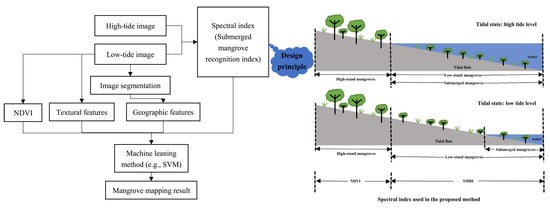
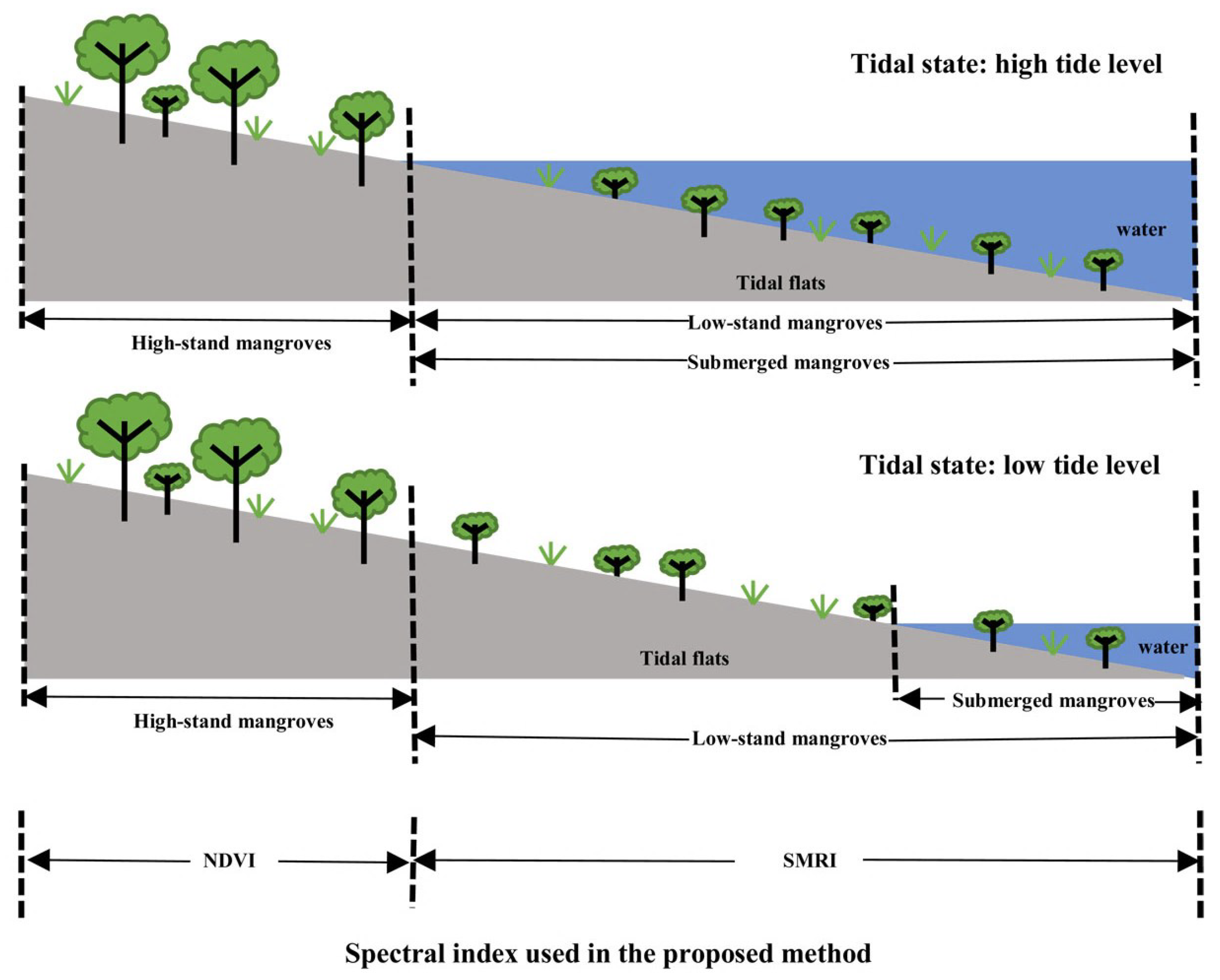
Mangrove forests are distributed in intertidal zones along nearshore coastlines, and thus low-stand mangrove forests are periodically submerged by variable tide levels at different times (Figure 1). With the fluctuating tide levels, mangrove forests show different spectral signatures, depending upon whether water is present or absent underneath the canopy of the mangrove forests. This characteristic of mangrove forests, which is different from that of other forest types, requires the development of a new method of mapping mangrove forests based on multi-tide satellite imagery.
If two images (high-tide and low-tide) of an area can be collected to analyze the difference of spectral signatures of the mangrove forests between the two tide states, a quantitative spectral index can be designed based on this difference to recognize mangrove forests in tidal zones. In this paper, such an index is called the “submerged mangrove recognition index” (SMRI). The detailed design of SMRI is presented in Section 3.2. Owing to the increased abundance of satellite and RS images, it is becoming progressively easier to collect available images of an area (even those with high spatial resolution) captured at (near) low tide and (near) high tide. This then makes it possible to calculate the SMRIs of mangrove forests quite practically.
The SMRI can be calculated from multi-tide, high-resolution images for use in recognizing submerged mangroves. In turn, the normalized difference vegetation index (NDVI), which is a spectral index widely used to separate vegetation from non-vegetation [49,50,51], can also be calculated as a spectral feature from one of the images (i.e., for low or high tide) to identify high-stand mangroves (Figure 1). Thus, these two indices can be applied in an advanced framework of object-based RS image classification via machine learning (e.g., SVM) for mapping mangrove forests. To further improve the mapping results, relevant textural and geographic features (e.g., homogeneity and contrast), which characterize the spatial distribution of mangrove forests, can also be used in this framework [14,52,53,54].
Such a method, which is based on multi-tide, high-resolution satellite imagery (Figure 2), is proposed in this paper to map mangrove forests (including those submerged during high tide) with a higher accuracy than existing methods that use single-tide imagery.
3. Materials and the Detailed Method
Based on the above-presented idea, in this section, we describe the detailed implementation of our proposed method with multi-tide, high-resolution images in a case study area.
3.1. Study Area and Data Preparation
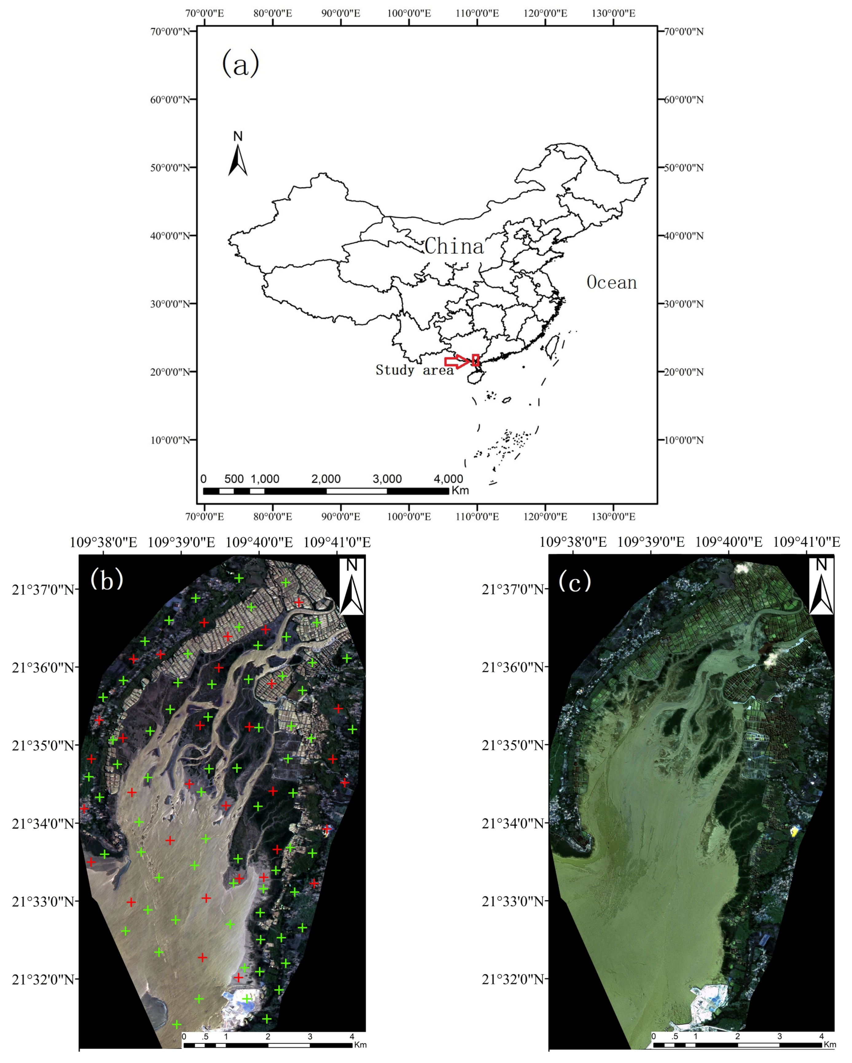
The study area is located in the Shankou National Mangrove Forest Nature Reserve, the west of the Shatian Peninsula in the Guangxi Zhuang Autonomous Region of China, within 109°38′–109°41′E longitude and 21°31′–21°37′N latitude (Figure 3a,b). There are five main land cover types in this study area: mangrove forests, tidal flats, water (ocean and pond), terrestrial vegetation, and built-up land. Mangrove forests in the study area are distributed in variety of settings, such as along the coastal fringe, and in extensive intertidal mudflats. The major species communities consist of Rhizophora stylosa, Bruguiera gymnorrhiza, Kandelia candel, Excoecaria agallocha, Aegiceras corniculatum, and Avicennia marina. The climate in this area is tropical monsoon, with an average annual temperature of 18 °C. The average annual rainfall is 1200–1800 mm. The hierarchy of mangrove forests is simple, and most exist as sparse patches. Meanwhile, the height of mangrove forests is usually less than 3.5 m in the study area. The tidal type is regularly diurnal, and tidal datum plane is 359 cm above the mean sea level. The study area experiences a large tidal range, with a maximum tide of 6.25 m, and it has a relatively stable mangrove ecosystem.
The 62 field sample points in this study were acquired from a field investigation in October 2017, and were recorded using the global positioning system (GPS). We also collected 38 sample points from images on Google Earth. All sample points for different land cover types were randomly divided into two sets, i.e., 32 training points, and 68 evaluation points for an accuracy assessment of the proposed method.
The high-resolution RS images used in this study are from the GF-1 satellite. The GF-1 satellite is the first of a series of Chinese, high-resolution satellites, which was launched on 26 April 2013. GF-1 images have a spatial resolution of 2 m in the panchromatic band (450–900 nm), and 8 m in the four multispectral bands (band 1: 450–520 nm; band 2: 520–590 nm; band 3: 630–690 nm; and band 4: 770–890 nm). Bands 1–3 are blue, green and red bands, respectively. Band 4 is near-infrared band. A panchromatic image and a multispectral image were obtained at the same time. The revisit cycle of GF-1 satellite is 41 days. GF-1 imagery was provided by the National Satellite Oceanic Application Center, China (http://dds.nsoas.org.cn/mainIndex.do).
Due to the long revisit cycle of GF-1 and the requirement of selecting cloud-free images, it is hard to acquire GF-1 satellite imagery precisely at the lowest tide. The GF-1 images selected for the proposed method should have as wide a tidal range as possible, which means that the phases of the low- and high-tide images should be as close to the lowest and highest tide levels, respectively, as possible. With this requirement in mind, two GF-1 images were acquired at (near) low tide of 289 cm on 2 June 2016 and (near) high tide of 398 cm on 31 August 2017 [55] (Figure 3b,c, respectively). Although there is a time lag of about one year between these two images, the spatial distribution of mangrove forests in this area was relatively stable during this period, according to our consulting with local authorities and local experts in the Guangxi Shankou National Mangrove Forest Nature Reserve Administration. As shown in Figure 3b,c, the fluctuating tide level has a significant effect on distinguishing mangrove forests because the low-stand mangrove is submerged by the high tide.
GF-1 images need a series of preprocessing procedures before their application for spectral index calculation and mangrove forest classification. First, radiometric corrections were conducted with the dark object subtraction algorithm to reduce atmospheric effects [56]. Then, the GF-1 images were geometrically corrected using the ENVI Rational polynomial coefficients (RPC) with 10 evenly spread ground control points extracted from a 1:50,000 topographic map. The average root mean square error (RMSE) was less than 1 pixel in both the X and Y directions. The nearest neighbor diffusion (NNDiffuse) pan-sharpening algorithm [57] was applied to image fusion. The NNDiffuse pan-sharpening algorithm assumes that the new spectrum value of each pixel in the high-resolution fused image is a weighted linear combination of its immediate neighboring superpixels in the multispectral image. The weights are determined by a diffusion model inferred from the panchromatic image, which estimates the similarity of the pixel of interest to its nine neighboring superpixels [57]. The spatial resolution of multispectral GF-1 images was enhanced to 2 m using NNDiffuse pan-sharpening algorithm to create a pan-sharpened, multispectral image. Radiometric corrections, geometric corrections, and image fusion were performed with the ENVI version 5.3 software (Exelis Visual Information Solutions Inc., Boulder, CO, USA).
3.2. Extraction of Spectral Indices
To determine the SMRIs mentioned in Section 2, which were used to quantify distinctive spectral characteristics of the submerged mangrove forests, we collected and analyzed the spectral signatures of low-stand and high-stand mangrove forests as well as four coexisting land-cover types (tidal flats, terrestrial vegetation, built-up land, and water; Table 1) from the GF-1 fused images in the study area. The sample points of these land cover types were acquired from the field survey data. For those inaccessible places, we collected the sample points from high-resolution images available from Google Earth. For each sample point, the location and land cover type were recorded. These sample points were representative of the distribution of mangrove forests and other land-cover types distributed near the mangrove forests in the study area. The number of sample points of the mangroves, tidal flats, terrestrial vegetation, built-up land, and water are 20, 12, 12, 11, and 13, respectively.
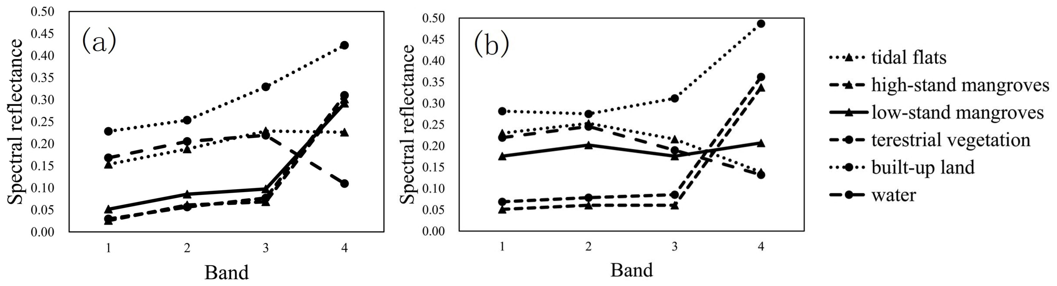
In this study, all operations and image analysis were based on fused images after NNDiffuse pan-sharpening algorithm, because NNDiffuse pan-sharpening algorithm can preserve spectral fidelity [58,59]. Figure 4 shows the spectral reflectance curves of different land cover types from GF-1 images before and after NNDiffuse pan-sharpening algorithm, based on the same sample points used in this study. As shown in Figure 4, there is minor difference in spectral reflectance values between the images before and after NNDiffuse pan-sharpening algorithm. This minor difference in spectral reflectance values would not affect spectral analysis and image classification results distinctly, while the image fusion can enhance the spatial resolution of multispectral GF-1 images to be higher (i.e., 2 m).
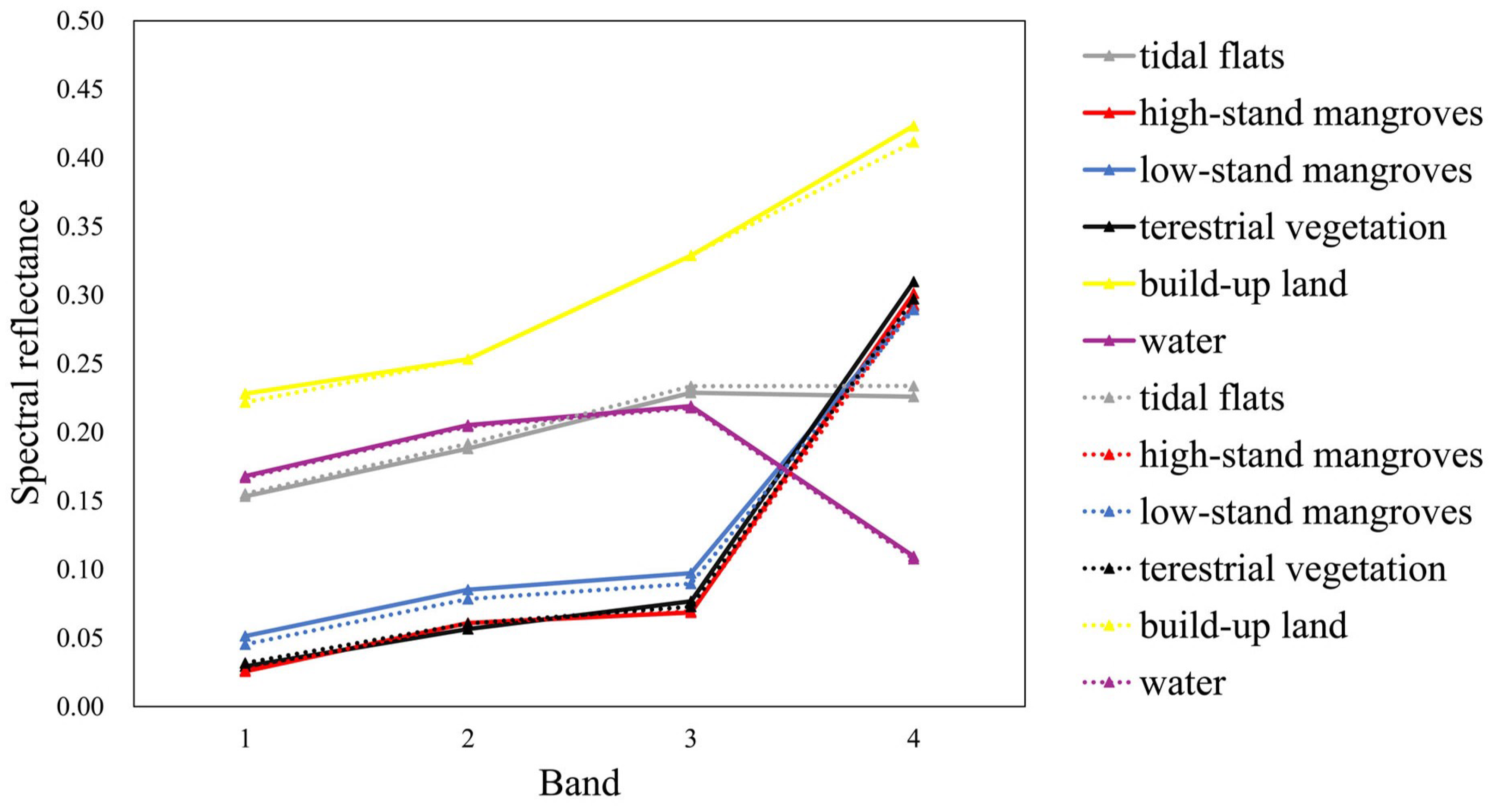
Figure 5 shows the spectral reflectance curves derived from the GF-1 images for each typical land-cover type under low and high tide, respectively. At low tide (Figure 5a), there are obvious spectral signature similarities between mangroves (including low-stand and high-stand mangroves) and terrestrial vegetation, which means there was a large amount of spectral overlap between them. The spectral signatures of tidal flats exhibit significant separation in the near-infrared band (i.e., band 4), while they have very similar spectral properties to water in bands 1–3.
At high tide, low-stand mangroves and tidal flats with a low elevation are inundated with increased tide levels. The spectral signatures of low-stand mangroves are primarily influenced by water. The spectral signatures of low-stand mangroves contain not only the spectral signatures of water, but also the spectral signatures of low-stand mangrove from underwater. Water has a higher reflectance than terrestrial vegetation in bands 1–3, and also has a lower reflectance than terrestrial vegetation in near-infrared band (band 4). The reflectance of low-stand mangroves is higher than that of terrestrial vegetation in bands 1–3, except in the near-infrared band (Figure 5b). The near-infrared band reflectance of low-stand mangroves at low tide is 40.9% of the corresponding value at high tide (Table 2). Tidal flats that were completely submerged due to low elevation coastal zones present a similar spectral signature to water. The near-infrared band reflectance of tidal flats at low tide was 63% of the corresponding value at high tide (Table 2). Both the tidal flats and low-stand mangroves exhibited spectral signature separation in the near-infrared band. In upper intertidal zones, the spectral differences of high-stand mangroves during high and low tide were lower than those for low-stand mangroves. However, the reflectance of high-stand mangroves was lower than terrestrial vegetation in all bands, which can likely be attributed to the effect of background reflectance of inundating tidal waters at high tide. Other land cover types had relatively stable reflectance values during high tide and low tide.
The above analysis shows that there is a distinct separation in the spectral properties in the near-infrared band for low-stand mangroves and tidal flats between low tide and high tide. Compared with bands 1–3, the near-infrared band is more sensitive to changes in vegetation/water content. In this study, water includes ocean and rivers (Table 1). Although clear water almost absorbs all the reflectance signal in near-infrared band, the reflectance of ocean and rivers (i.e., the “water” type in this study) in near-infrared band is not zero, due to the presence of suspended sediments, low-stand mangrove, etc. Therefore, the near-infrared band can be used as a vegetation/water content indicator for the SMRI to distinguish any submerged mangroves in multi-tide imagery [60,61,62].
The detailed form of the SMRI was further explored based on a combination of above analysis and the NDVI:
where , are the reflectance values in the near-infrared and red bands, respectively. Table 3 presents the NDVI statistical results and its derived spectral indices for each land-cover type from the GF-1 images at low tide and high tide. The NDVI values of vegetation (such as terrestrial vegetation, high-stand mangroves, and low-stand mangroves) were higher than those of other classes at low tide. The NDVI values of nearshore land-cover types (especially low-stand mangroves) have a clear change from low tide to high tide, due to the change of tide level. As shown in Table 3, the difference in the absolute NDVI values of the low-stand mangroves between low and high tide is greater than 0.41, while those of other land-cover types are all less than 0.21. This difference can be used to identify low-stand mangroves.
As low-stand mangroves are submerged by high tide levels, their spectral signatures are characterized not only by water content, but also vegetation. Based on the above analysis, the SMRI is designed to describe the unique spectral signature of submerged mangroves and to distinguish mangroves submerged by high- and low-tide levels:
where NDVIl and NDVIh are NDVI values at low tide and high tide, respectively, and NIRl and NIRh are the reflectance of the near-infrared band at low and high tide, respectively.
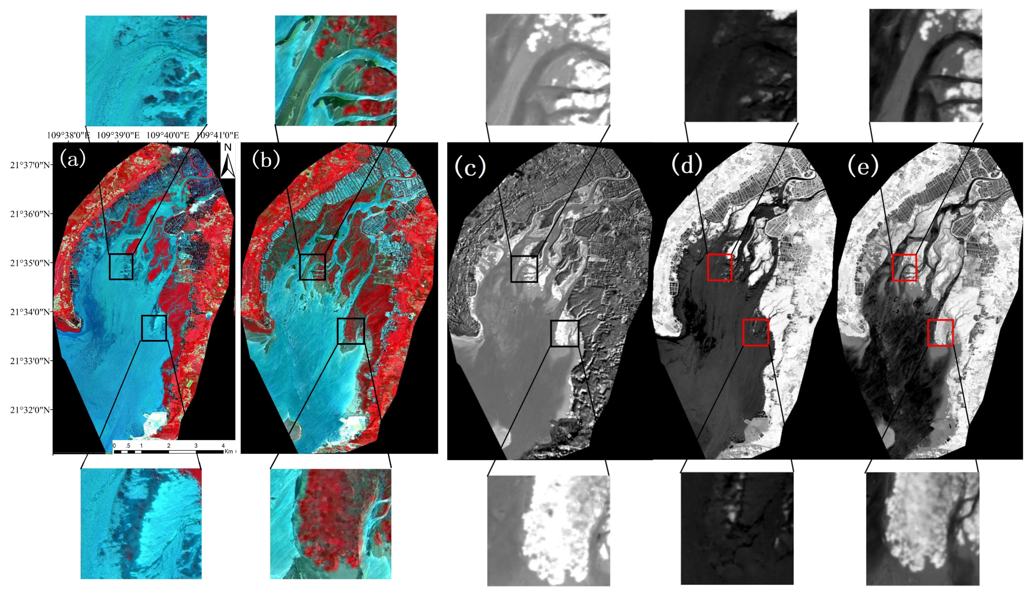
We calculated SMRI and NDVI images at high and low tide (Figure 6). In the NDVI images, vegetation cover is white (Figure 6d,e), and the larger the vegetation cover is, the greater the NDVI value becomes. In the SMRI image, the submerged mangroves are white (Figure 6c). For submerged mangroves in high-tide images, they are black in the NDVI image and it is difficult to distinguish the submerged mangroves. However, the SMRI was created to optimize our ability to identify submerged mangroves, which was hence utilized as the differentiating spectral feature for submerged mangroves at high tide. The SMRI highlights the difference between mangrove forests and water, which can comparatively reduce the confusion caused by high tide levels.
3.3. Textural Feature Extraction
In addition to the NDVIs and SMRIs, textural information is an intrinsic feature needed to distinguish mangrove forests from vegetation, especially for cases where the land cover has a similar spectral response as mangrove forests. Using textural features within a classifier can enhance the classification accuracy in mangrove forest mapping [14,63,64,65,66,67]. The grey level co-occurrence matrix (GLCM) proposed by Haralick et al. has been proven to be a powerful tool for RS image texture analysis [68]. A GLCM is created by calculating how often pairs of pixel with specific values and with a specified spatial relationship occur in a grey image. Then, statistical measures are calculated based on this matrix to provide information about the texture of an image, such as the shape, size and the spatial relationships of pixels within the image.
Haralick et al. proposed 14 original statistics to be applied to the GLCM to measure texture features. Among these features, homogeneity, contrast, entropy, and correlation have been reported to be effective in discriminating spatially heterogeneous images [69,70,71]. In this study, these four textural features were adopted in our proposed method as input features of a classifier, which were calculated as follows:
where p(i,j) are the pixel values of the co-occurrence matrix; p(i) and p(j) are the row and column values of the co-occurrence matrix, respectively; and , , are the means and standard deviations of p(i) and p(j), respectively.
3.4. Object-Based Classification with an SVM
An SVM is a fast and efficient machine-learning algorithm [72,73,74,75]. Based on statistical learning theory, an SVM creates a hyperplane in an N-dimensional spectral space, which separates any classes by maximizing the margin between them. The data points closest to the hyperplane (the so-called optimal hyperplane) are named as support vectors. There are four types of kernels which could be used in an SVM: linear, polynomial, a radial basis function, and sigmoid. Among them, the radial basis function has been found to work best in most cases [73,76] and is adopted in our proposed method. The SVM classifier was operated in eCognition Developer 9.0 for training and classification.
Object-based classification includes two steps: image segmentation, and classification. Image segmentation is the process whereby a group of pixels that have similar spectral and spatial properties is considered as an object [77,78,79,80]. For more detailed information about image segmentation, see Myint et al. [81].
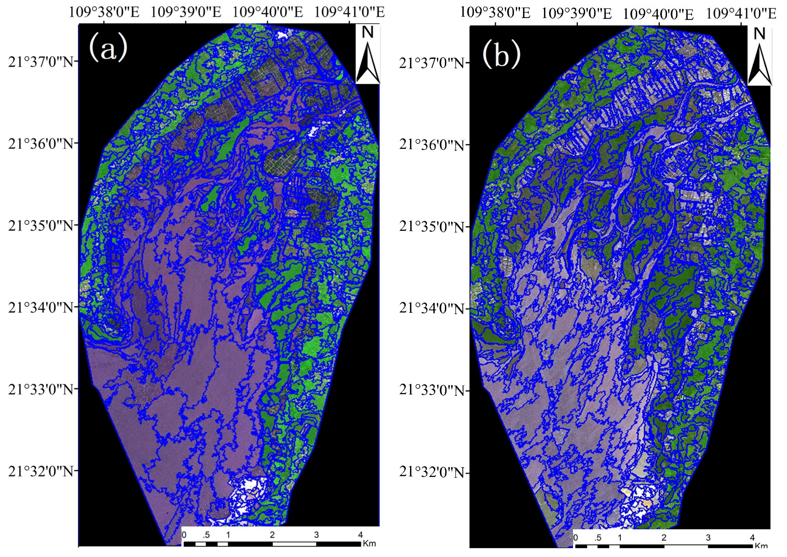
A series of segmentations were conducted using eCognition Developer 9.0, which is an image analysis program. First, high- and low-tide images were segmented into homogeneous objects based on several criteria including color, shape, size, and context. There are three parameters that control the outcome of the segmentation: scale, shape, and compactness [77,78,79,80]. Scale is indirectly related to the average size of the created object. Shape balances the spectral homogeneity and the shape of objects. Compactness balances the compactness and smoothness. Starting with low parameter values, a set of parameters was adjusted until the created objects represented the smallest isolated mangrove community patches. After a series of tests, a satisfactory match was obtained for this case study when the scale, shape and compactness parameters were 900, 0.1, and 0.5, respectively (Figure 7).
After image segmentation, the SVM classifier with a radial basis function had two hyperparameters which need to be tuned for good performance, i.e., a regularization constant C, and a kernel hyperparameter . The Grid Search algorithm [82] was used to tune these hyperparameters for the optimum values, that is C = 2 and in this case study. The spectral features (i.e., NDVI and SMRI) and textural features were aligned with the spectral features from the sharpened images to form a higher dimension feature vector as an input into the SVM classifier. These features and the original spectral features had the same weighting. The classification results included five land-cover types: mangroves, tidal flats, terrestrial vegetation, water and built-up land, where the latter four were classified as “non-mangrove”.
A detailed land cover map for 2017 was provided by the authorities in the Guangxi Shankou National Mangrove Forest Nature Reserve Administration. The land cover types include water, tidal flats, mangrove forests, ponds, terrestrial vegetation, built-up land, farmland, etc. As mangrove forests grow up in tidal flats along coastlines, geographic features can be used to improve classification results. The maximum distance to the water was set to 2.5 km after visual interpretation trials in this study. The restriction of the maximum distance to the water can help to avoid the confusion between mangrove forests and terrestrial vegetation. Besides, from the low-tide sharpened image, mangrove forests were adjacent to tidal flats or the water (Figure 3b). From the high-tide sharpened image, low-stand mangroves were submerged or adjacent to the water (Figure 3c). Therefore, the geographic feature that a mangrove should share a border with a tidal flat or water was used to assist with mangrove classification in this study.
The proposed method was implemented via the above processes based on multi-tide, high-resolution images, which can successfully distinguish mangrove forests in the case study area.
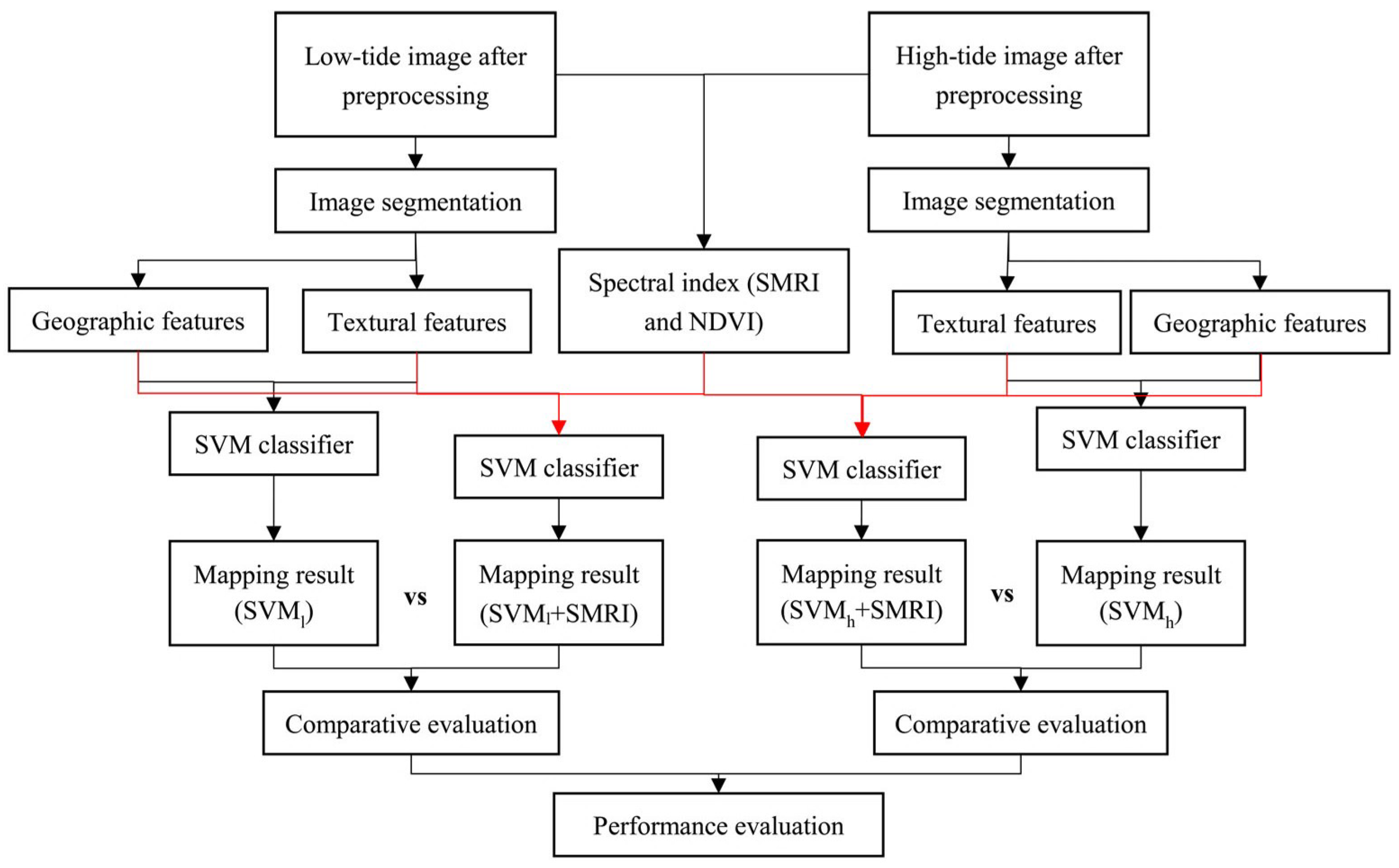
4. Evaluation Method
In this study, the proposed method that includes SMRIs and the other features (i.e., NDVI, textural and geographic features) extracted from high-tide images, hereinafter called “SVMh + SMRI” for short, was compared with an existing method that uses object-based SVM classifier with NDVI values, along with textural and geographic features extracted from high-tide image (i.e., just SVMh values) (see Figure 8). Similarly, the proposed method (“SVMl + SMRI”) was also compared with an existing method that considers NDVI values, as well as textural and geographic features extracted from low-tide images (i.e., just SVMl values). This comparison aims to evaluate the effectiveness of our proposed method, especially for submerged mangrove forests.
The results from the SVMh + SMRI method was also compared with that from the SVMl + SMRI method (Figure 8). The aim of this comparison is to highlight the effect of using NDVI along with textural and geographic features extracted from just high-tide or low-tide images on our proposed method.
In addition to the visual interpretation and qualitative discussion of the spatial distribution of mangrove forests mapped by each method under consideration, a quantitative accuracy evaluation of each resultant map from each method was conducted via a confusion matrix showing user’s accuracy, producer’s accuracy, and overall accuracy, which is the normal way used for accuracy assessment of mangrove and non-mangrove classification [2,4]. The confusion matrix was generated using all the validation data. Since mapping mangrove forests is the focus of this study, the validation data were reclassified into two classes: mangrove and non-mangrove. The quantitative indices of the accuracy evaluation used in this study include the overall accuracy, the producer’s accuracy, the user’s accuracy, and the Kappa coefficient. The area of the mangrove forests mapped by each method was also calculated for a comprehensive comparison.
5. Results and Discussion
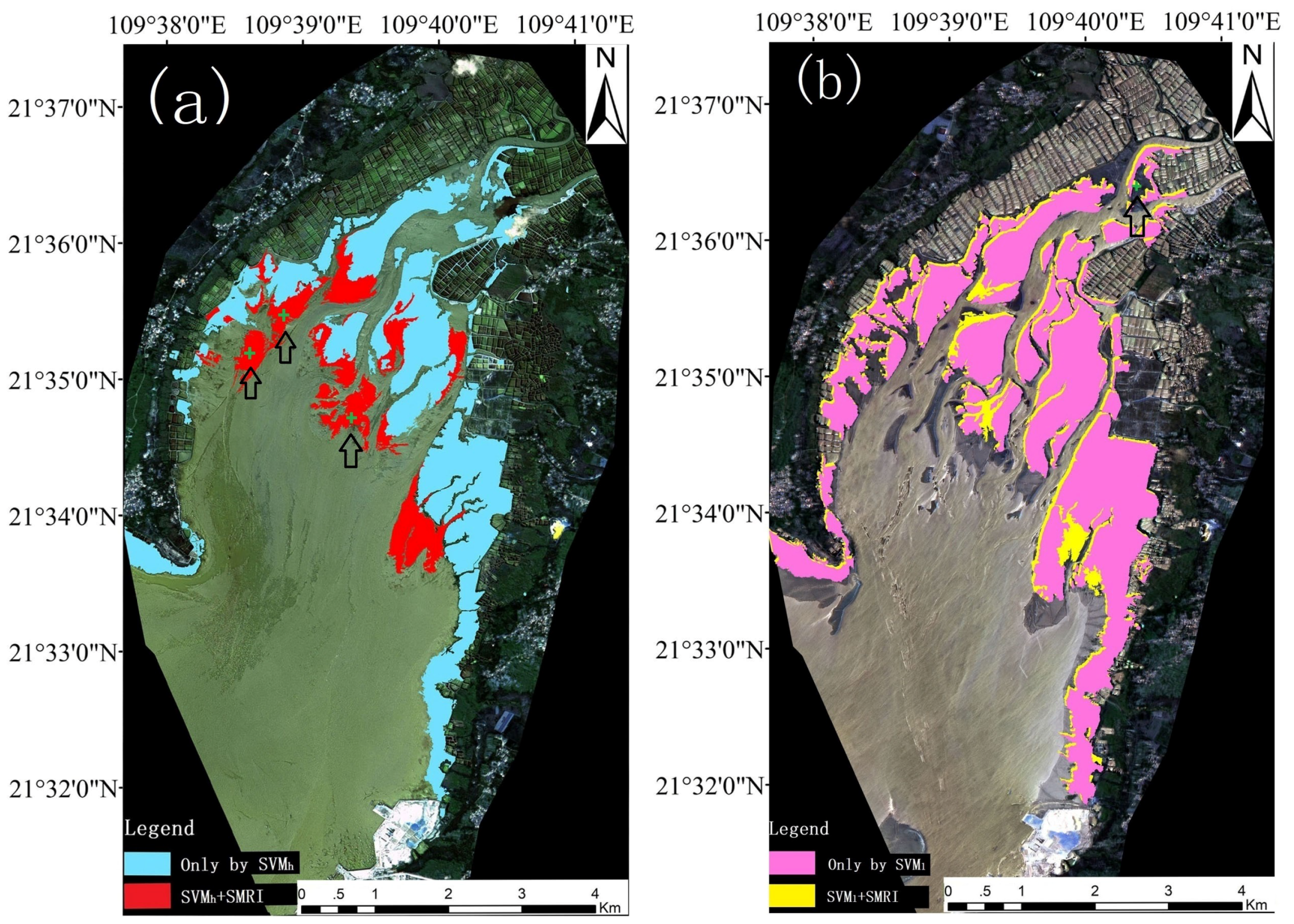
Figure 9 illustrates the classification results of the four different methods.
Mangrove forests are periodically submerged by incoming tides. Depending on the tide levels, underlying sediment or inundating tidal waters influence their spectral signatures and confound the differentiation of mangroves from other adjoining vegetation classes. From the classification results of SVMh and SVMh + SMRI, it can be found that the submerged mangrove forests were effectively distinguished and classified as mangrove forests by the proposed method when using high-tide images (i.e., SVMh + SMRI) (Figure 9a). Without the use of SMRI, the classification result from SVMh (the blue area in Figure 9a) shows that mangrove forests above the water were classified as mangroves; however, the submerged mangrove forests were not distinguished by the SVMh. For example, three evaluation points marked in Figure 9a were correctly classified as mangroves by SVMh + SMRI (as well as SVMl + SMRI) and incorrectly classified as non-mangrove (i.e., water) by the SVMh. Hence, the classification result of mangrove forests can be greatly improved by the proposed method. In terms of visual interpretation, the classified mangrove forests from each method were mainly distributed along coastlines, and some sparse mangrove forests were distributed in low tidal flats. The classification results from the proposed method (SVMh + SMRI or SVMl + SMRI) showed an overall agreement with the field investigation.
A small number of the terrestrial vegetation patches at landward margins were incorrectly classified as mangrove forests by the proposed method. This is mainly because the spectral signatures of mangroves are similar to those of adjoining terrestrial vegetation, and the spectral signatures of terrestrial vegetation are strongly influenced by underlying ponds. As such, a great deal of adjoining terrestrial vegetation was easily misclassified as mangrove forests. However, the incorporation of geographical features excluded a lot of terrestrial vegetation, and reduced the number of errors compared to the other methods.
Next are the classification results of SVMl and SVMl + SMRI on the low-tide images, where most of mangrove forests were not submerged. Here, the SVMl correctly classified most mangrove forests. For those mangroves that were sparsely distributed on tidal flats or slightly submerged, they can be distinguished with SVMl + SMRI. One evaluation point marked in Figure 9b was correctly classified as mangrove by SVMl + SMRI and incorrectly classified as non-mangrove by the SVMl as well as SVMh + SMRI. It was proven that SMRI not only distinguishes submerged mangroves, but also effectively discriminates slightly submerged mangroves.
The confusion matrix from the accuracy assessment demonstrates that the overall agreement between the classification results of the proposed method and the field investigation data was satisfactory (Table 4). The overall accuracy was 94% and the Kappa coefficient was 0.86 for SVMl + SMRI, which achieved the best accuracy of the tested methods. SVMh + SMRI achieved a lower overall accuracy and Kappa coefficient (91%, 0.79) than SVMl + SMRI. Moreover, the SVMl values showed even lower accuracies, (86% overall accuracy) and Kappa coefficient (0.68). The SVMh had the lowest overall accuracy and Kappa coefficient among these methods. The producer’s accuracy and user’s accuracy of mangrove forests of SVMh + SMRI were 0.85 and 0.85, respectively. These dropped to 0.70 and 0.74 for SVMh, respectively. This large reduction in confusion between mangroves and non-mangroves represents a major advantage of using SMRI features in the SVM classifier. The proposed method not only greatly improves the classification performance of the SVM classifier, but it can also accurately distinguish mangrove forests from other land cover classes, especially for submerged mangroves at high tide.
Note that Zhang et al. [2] used the decision tree method with the dataset of Digital Elevation Model (DEM), NDVI and NDMI to map mangrove forests from two Landsat images which were captured at two tide levels in their case study. Here, we compare Zhang et al’s. [2] results with the results at low tide from the proposed method in this study. In Zhang et al. [2] research results, the producer’s accuracy and user’s accuracy were 91.8% and 85.7% from Landsat TM, and 90.7% and 90.1% from Landsat 8 Operational Land Imager (OLI), respectively. The producer’s accuracy and user’s accuracy from the proposed method (SVMl + SMRI) were 90%, and 90%, respectively. The producer’s accuracy and user’s accuracy from Zhang et al. [2] were almost the same as those from the proposed method in this study. However, the proposed method produced an improved accuracy in overall accuracy and Kappa (i.e., 94% and 0.86 from SVMl + SMRI), which are higher than those from Landsat TM (92.5% and 0.83) and from Landsat OLI (93.8% and 0.858) in [2]. In addition, the decision tree method used by Zhang et al. [2] for distinguishing mangroves is largely depended on the quality of the constructed decision tree. For each layer of the decision tree, it must be set with different thresholds to differentiate different land cover types. The thresholds were determined by the visual interpretation on the characteristics of different land cover types. Therefore, the decision tree method is difficult to automate and its classification accuracy largely depends on the quality of the visual interpretation. The proposed method in this paper used a fast and efficient SVM classifier, and thus achieved an automated procedure for distinguishing mangrove forests.
Table 4 also lists the area of mangrove forests mapped by the different methods under consideration. The total area of mangrove forests was 911.952, 860.708, 799.274, and 594.222 ha for SVMl + SMRI, SVMl, SVMh + SMRI, and SVMh, respectively. It can be found that the calculated area of mangroves in the low-tide images was larger than those in the high-tide images. Although the SMRI index can distinguish submerged mangrove forests at high tide, the total area at high tide was still underestimated. The reason for this is that low-stand mangroves along coastlines were totally submerged due to the high tide levels, resulting in changes of the spectral signature from mangrove forests to water. The spectral signature of seaward low-stand mangroves when were deeply submerged by water became the spectral signature of water, which cannot be distinguished by the SMRI index. The spectral signature of landward low-stand mangroves which were slightly submerged by water reflected the spectral signatures of both water and underlying low-stand mangroves. Thus, these submerged mangroves can be distinguished by the SMRI index. The area of mangrove forests from the SVMl + SMRI method was 51.244 ha larger than that from the SVMl. It is demonstrated that some submerged mangrove forests that are sparsely distributed on tidal flats were distinguished with the incorporation of the SMRI. The area of mangrove forests from the SVMh + SMRI method was 205.052 ha larger than that from the SVMh. It can be seen that many submerged mangrove forests were effectively distinguished, attributed to the application of the SMRI index together with the proposed method. Hence, the SMRI is an effective index that helps to distinguish submerged mangrove forests.
6. Conclusions
To date, tidal effects have been a significant limitation for accurately mapping mangrove forests, particularly in China where species diversity is high and the distribution of mangroves is sparse. We proposed an object-based SVM method for mapping mangrove forests using multi-tide, high-resolution RS imagery (GF-1). In the proposed method, a new spectral index, the SMRI, which is based on high-tide and low-tide images, was designed to enhance the separability of submerged mangrove forests. This was then used together with the NDVI, and textural and geographic features to improve the mapping result.
The evaluation results show that the introduction of the SMRI greatly improved the identification accuracy, especially for submerged mangrove forests. The proposed method of mapping mangrove forests based on multi-tide, high-resolution satellite imagery achieved a satisfactory mapping result and higher classification accuracies in the study area compared with those from existing methods that only use single-tide imagery.
Author Contributions
Q.X. and C.-Z.Q. conceived the whole research, designed the proposed method, and wrote the manuscript. H.L., C.H. and F.-Z.S. contributed to the evaluation of the proposed method and checked the writing of the manuscript.
Funding
This research was funded by the Science and Technology Basic Resources Investigation Program of China (No. 2017FY100706).
Acknowledgments
The authors thank all members of their research group for their great help in the field investigation. The authors are also grateful to the authorities in the Guangxi Shankou National Mangrove Forest Nature Reserve Administration for kindly providing a detailed land cover map in 2017 and consultations. The authors thank anonymous reviewers for their constructive comments which are helpful to improve this manuscript.
Conflicts of Interest
The authors declare no conflict of interest.
References
- Giri, C.; Long, J.; Tieszen, L. Mapping and Monitoring Louisiana’s Mangroves in the Aftermath of the 2010 Gulf of Mexico Oil Spill. J. Coast. Res. 2011, 277, 1059–1064. [Google Scholar] [CrossRef]
- Zhang, X.; Treitz, P.; Chen, D.; Quan, C.; Shi, L.; Li, X. Mapping mangrove forests using multi-tidal remotely-sensed data and a decision-tree based procedure. Int. J. Appl. Earth Obs. Geoinf. 2017, 62, 201–214. [Google Scholar] [CrossRef]
- Jia, M.; Wang, Z.; Zhang, Y.; Ren, C.; Song, K. Landsat-based estimation of mangrove forest loss and restoration in Guangxi province, China, influenced by human and natural factors. IEEE J. Sel. Top. Appl. Earth Obs. 2015, 8, 311–323. [Google Scholar] [CrossRef]
- Vo, Q.; Oppelt, N.; Leinenkugel, P.; Kuenzer, C. Remote sensing in mapping mangrove ecosystems—An object-based approach. Remote Sens. 2013, 5, 183–201. [Google Scholar] [CrossRef] [Green Version]
- Kuenzer, C.; Bluemel, A.; Gebhardt, S.; Quoc, T.; Dech, S. Remote Sensing of Mangrove Ecosystems: A Review. Remote Sens. 2011, 3, 878–928. [Google Scholar] [CrossRef] [Green Version]
- Walters, B.; Ronnback, P.; Kovacs, J.; Crona, B.; Hussain, S.; Badola, R.; Primavera, J.; Barbier, E.; Dahdouh-Guebas, F. Ethnobiology, socio-economics and management of mangrove forests: A review. Aquat. Bot. 2008, 89, 220–236. [Google Scholar] [CrossRef] [Green Version]
- Abd-El Monsef, H.; Smith, S. A new approach for estimating mangrove canopy cover using Landsat 8 imagery. Comput. Electron. Agric. 2017, 135, 183–194. [Google Scholar] [CrossRef]
- Jia, M.; Wang, Z.; Li, L.; Song, K.; Ren, C.; Liu, B.; Mao, D. Mapping China’s mangroves based on an object-oriented classification of Landsat imagery. Wetlands 2014, 34, 277–283. [Google Scholar] [CrossRef]
- Giri, C.; Zhu, Z.; Tieszen, L.; Singh, A.; Gillette, S.; Kelmelis, J. Mangrove forest distributions and dynamics (1975–2005) of the tsunami-affected region of Asia. J. Biogeogr. 2008, 35, 519–528. [Google Scholar] [CrossRef] [Green Version]
- Lovelock, C.; Cahoon, D.; Friess, D.; Guntenspergen, G.; Krauss, K.; Reef, R.; Rogers, K.; Saunders, M.; Sidik, F.; Swales, A.; et al. The vulnerability of Indo-Pacific mangrove forests to sea-level rise. Nature 2015, 526, 559–563. [Google Scholar] [CrossRef] [PubMed] [Green Version]
- Kirui, K.; Kairo, J.; Bosire, J.; Viergever, K.; Rudra, S.; Huxham, M.; Briers, R. Mapping of mangrove forest land cover change along the Kenya coastline using Landsat imagery. Ocean Coast. Manag. 2013, 83, 19–24. [Google Scholar] [CrossRef] [Green Version]
- Long, J.; Giri, C. Mapping the Philippines’ mangrove forests using Landsat imagery. Sensors 2011, 11, 2972–2981. [Google Scholar] [CrossRef] [PubMed]
- Everitt, J.; Yang, C.; Sriharan, S.; Judd, F. Using High Resolution Satellite Imagery to Map Black Mangrove on the Texas Gulf Coast. J. Coast. Res. 2008, 246, 1582–1586. [Google Scholar] [CrossRef]
- Wang, T.; Zhang, H.; Lin, H.; Fang, C. Textural–Spectral Feature-Based Species Classification of Mangroves in Mai Po Nature Reserve from Worldview-3 Imagery. Remote Sens. 2016, 8, 24. [Google Scholar] [CrossRef]
- Xun, L.; Wang, L. An object-based SVM method incorporating optimal segmentation scale estimation using Bhattacharyya Distance for mapping salt cedar (Tamarisk spp.) with QuickBird imagery. GISci. Remote Sens. 2015, 52, 257–273. [Google Scholar] [CrossRef]
- Heenkenda, M.; Joyce, K.; Maier, S.; Bartolo, R. Mangrove species identification: Comparing WorldView-2 with aerial photographs. Remote Sens. 2014, 6, 6064–6088. [Google Scholar] [CrossRef]
- Kux, H.; Souza, U. Object-based image analysis of WORLDVIEW-2 satellite data for the classification of mangrove areas in the city of São Luís, Maranhão State, Brazil. ISPRS Ann. Photogramm. Remote Sens. Spat. Inf. Sci. 2012, 4, 95–100. [Google Scholar] [CrossRef]
- Malinverni, E.; Tassetti, A.; Mancini, A.; Zingaretti, P.; Frontoni, E.; Bernardini, A. Hybrid object-based approach for land use/land cover mapping using high spatial resolution imagery. Int. J. Geogr. Inf. Sci. 2011, 25, 1025–1043. [Google Scholar] [CrossRef]
- Manson, F.; Loneragan, N.; Mcleod, I.; Kenyon, R. Assessing techniques for estimating the extent of mangroves: Topographic maps, aerial photographs and Landsat TM images. Mar. Freshw. Res. 2001, 52, 787–792. [Google Scholar] [CrossRef]
- Heumann, B. Satellite remote sensing of mangrove forests: Recent advances and future opportunities. Prog. Phys. Geogr. 2011, 35, 87–108. [Google Scholar] [CrossRef]
- Mitra, D.; Karmaker, S. Mangrove Classification in Sundarban using High Resolution Multi-Spectral Remote Sensing Data and GIS. Asian J. Environ. Disaster Manag. 2010, 2, 197. [Google Scholar] [CrossRef]
- Neukermans, G.; Dahdouh-Guebas, F.; Kairo, J.; Koedam, N. Mangrove species and stand mapping in Gazi Bay (Kenya) using Quickbird satellite imagery. J. Spat. Sci. 2008, 53, 75–86. [Google Scholar] [CrossRef]
- Green, E.; Clark, C.; Mumby, P.; Edwards, A.; Ellis, A. Remote sensing techniques for mangrove mapping. Int. J. Remote Sens. 1998, 19, 935–956. [Google Scholar] [CrossRef] [Green Version]
- Giri, C.; Pengra, P.; Zhu, Z.; Singh, A.; Tieszen, L. Monitoring mangrove forest dynamics of the Sundarbans in Bangladesh and India using multi-temporal satellite data from 1973 to 2000. Est. Coast. Shelf Sci. 2007, 73, 91–100. [Google Scholar] [CrossRef]
- Everitt, J.; Judd, F.; Escobar, D.; Davis, M. Integration of remote sensing and spatial information technologies for mapping black mangrove on the Texas gulf coast. J. Coast. Res. 1996, 12, 64–69. [Google Scholar]
- Li, M.; Lee, S. Mangroves of China: A brief review. For. Ecol. Manag. 1997, 96, 241–259. [Google Scholar] [CrossRef]
- Alongi, D. Present state and future of the world’s mangrove forests. Environ. Conserv. 2002, 29, 331–349. [Google Scholar] [CrossRef]
- Hernández Cornejo, R.; Koedam, N.; Ruiz Luna, A.; Troell, M.; Dahdouh-Guebas, F. Remote sensing and ethnobotanical assessment of the mangrove forest changes in the Navachiste-San Ignacio-Macapule lagoon complex, Sinaloa, Mexico. Ecol. Soc. 2005, 10, 16. [Google Scholar] [CrossRef]
- Helmer, E.; Kennaway, T.; Pedreros, D. Land cover and forest formation distributions for St. Kitts, Nevis, St. Eustatius, Grenada and Barbados from decision tree classification of cloud-cleared satellite imagery. Caribb. J. Sci. 2008, 44, 175–198. [Google Scholar] [CrossRef]
- Pal, M.; Mather, P. Support vector machines for classification in remote sensing. Int. J. Remote Sens. 2005, 26, 1007–1011. [Google Scholar] [CrossRef]
- Yu, X.; Shao, H.; Liu, X.; Zhao, D. Applying Neural Network Classification to Obtain Mangrove Landscape Characteristics for Monitoring the Travel Environment Quality on the Beihai Coast of Guangxi, PR China. CLEAN–Soil Air Water 2010, 38, 289–295. [Google Scholar] [CrossRef]
- Wang, L.; Silván-Cárdenas, J.; Sousa, W. Neural network classification of mangrove species from multi-seasonal Ikonos imagery. Photogram. Eng. Rem. Sens. 2008, 74, 921–927. [Google Scholar] [CrossRef]
- Gao, J.; Chen, H.; Zhang, Y.; Zha, Y. Knowledge-based approaches to accurate mapping of mangroves from satellite data. Photogram. Eng. Remote Sens. 2004, 70, 1241–1248. [Google Scholar] [CrossRef]
- Foody, G.; Mathur, A. The use of small training sets containing mixed pixels for accurate hard image classification: Training on mixed spectral responses for classification by a SVM. Remote Sens. Environ. 2006, 103, 179–189. [Google Scholar] [CrossRef]
- Xin, H.; Zhang, L.; Wang, L. Evaluation of Morphological Texture Features for Mangrove Forest Mapping and Species Discrimination Using Multispectral IKONOS Imagery. IEEE Geosci. Remote Sens. 2009, 6, 393–397. [Google Scholar] [Green Version]
- Li, H.; Fu, H.; Han, Y.; Yang, J. Object-oriented classification of high-resolution remote sensing imagery based on an improved colour structure code and a support vector machine. Int. J. Remote Sens. 2010, 31, 1453–1470. [Google Scholar] [CrossRef]
- Harken, J.; Sugumaran, R. Classification of Iowa Wetlands Using an Airborne Hyperspectral Image: A Comparison of the Spectral Angle Mapper Classifier and an Object- Oriented Approach. Can. J. Remote Sens. 2005, 31, 167–174. [Google Scholar] [CrossRef]
- Kumar, L.; Sinha, P. Mapping Salt-Marsh Land-Cover Vegetation Using High-Spatial and Hyperspectral Satellite Data to Assist Wetland Inventory. GISci. Remote Sens. 2014, 51, 483–497. [Google Scholar] [CrossRef]
- Kamal, M.; Phinn, S. Hyperspectral data for mangrove species mapping: A comparison of pixel-based and object-based approach. Remote Sens. 2011, 3, 2222–2242. [Google Scholar] [CrossRef]
- Kanniah, K.; Wai, N.; Shin, A.; Rasib, A. Per-pixel and sub-pixel classifications of high-resolution satellite data for mangrove species mapping. Appl. GIS 2007, 3, 1–22. [Google Scholar]
- Wang, L.; Sousa, W.; Gong, P. Integration of object-based and pixel-based classification for mapping mangroves with IKONOS imagery. Int. J. Remote Sens. 2004, 25, 5655–5668. [Google Scholar] [CrossRef]
- Genelett, D.; Gorte, B. A method for object-oriented land cover classification combining Landsat TM data and aerial photographs. Int. J. Remote Sens. 2003, 24, 1273–1286. [Google Scholar] [CrossRef]
- Conchedda, G.; Durieux, L.; Mayaux, P. An object-based method for mapping and change analysis in mangrove ecosystems. ISPRS J. Photogram. Remote Sens. 2008, 63, 578–589. [Google Scholar] [CrossRef]
- Flores De Santiago, F.; Kovacs, J.; Lafrance, P. An object-oriented classification method for mapping mangroves in Guinea, West Africa, using multipolarized ALOS PALSAR L-band data. Int. J. Remote Sens. 2013, 34, 563–586. [Google Scholar] [CrossRef]
- Li, M.; Mao, L.; Shen, W.; Liu, S.; Wei, A. Change and fragmentation trends of Zhanjiang mangrove forests in southern China using multi-temporal Landsat imagery (1977–2010). Estuar. Coast. Shelf Sci. 2013, 130, 111–120. [Google Scholar] [CrossRef]
- Rogers, K.; Lymburner, L.; Salum, R.; Brooke, B.; Woodroffe, C. Mapping of mangrove extent and zonation using high and low tide composites of Landsat data. Hydrobiologia 2017, 803, 49–68. [Google Scholar] [CrossRef]
- Collins, D.; Avdis, A.; Allison, P.; Johnson, H.; Hill, J.; Piggott, M.; Hassan, M.; Damit, A. Tidal dynamics and mangrove carbon sequestration during the Oligo–Miocene in the South China Sea. Nat. Commun. 2017, 8, 15698. [Google Scholar] [CrossRef] [PubMed] [Green Version]
- Li, S.; Tian, Q.; Yu, T.; Gu, X. The extraction of mangrove within intertidal zone based on multi-temporal HJ CCD images. In Proceedings of the 17th China Conference on Remote Sensing, Beijing, China, 27–31 August 2010. [Google Scholar]
- Satyanarayana, B.; Mohamad, K.; Idris, I.; Husain, M.; Dahdouh-Guebas, F. Assessment of mangrove vegetation based on remote sensing and ground-truth measurements at Tumpat, Kelantan Delta, East Coast of Peninsular Malaysia. Int. J. Remote Sens. 2011, 32, 1635–1650. [Google Scholar] [CrossRef]
- Nardin, W.; Locatelli, S.; Pasquarella, V.; Rulli, M.; Woodcock, C.; Fagherazzi, S. Dynamics of a fringe mangrove forest detected by Landsat images in the Mekong River Delta, Vietnam. Earth Surf. Proc. Landf. 2016, 41, 2024–2037. [Google Scholar] [CrossRef]
- Giri, S.; Mukhopadhyay, A.; Hazra, S.; Mukherjee, S.; Roy, D.; Ghosh, S.; Ghosh, T.; Mitra, D. A study on abundance and distribution of mangrove species in Indian Sundarban using remote sensing technique. J. Coast. Conserv. 2014, 18, 359–367. [Google Scholar] [CrossRef]
- Huang, X.; Liu, X.; Zhang, L. A multichannel gray level co-occurrence matrix for multi/hyperspectral image texture representation. Remote Sens. 2014, 6, 8424–8445. [Google Scholar] [CrossRef]
- Dian, Y.; Li, Z.; Pang, Y. Spectral and texture features combined for forest tree species classification with airborne hyperspectral imagery. J. Indian Soc. Remote Sens. 2015, 43, 101–107. [Google Scholar] [CrossRef]
- Szantoi, Z.; Escobedo, F.; Abd-Elrahman, A.; Smith, S.; Pearlstine, L. Analyzing fine-scale wetland composition using high resolution imagery and texture features. Int. J. Appl. Earth Observ. 2013, 23, 204–212. [Google Scholar] [CrossRef]
- National Marine Data and Information Service. Tide Tables, 1st ed.; Ocean Press: Beijing, China, 2016 and 2017; pp. 439–450. ISBN 978-7-5027-9129-2. [Google Scholar]
- Song, C.; Woodcock, C.; Seto, K.; Lenney, M.; Macomber, S. Classification and change detection using Landsat TM data: When and How to correct atmospheric effects? Remote Sens. Environ. 2001, 75, 230–244. [Google Scholar] [CrossRef]
- Sun, W.; Chen, B.; Messinger, D. Nearest-neighbor diffusion-based pan-sharpening algorithm for spectral images. Opt. Eng. 2014, 53, 013107. [Google Scholar] [CrossRef] [Green Version]
- Dorado-Munoz, L.; Messinger, D.; Bove, D. Integrating spatial and spectral information for enhancing spatial features in the Gough map of Great Britain. J. Cult. Herit. 2018. Available online: https://www.sciencedirect.com/science/article/pii/S1296207417307008 (accessed on 9 August 2018).
- Zhao, J.; Huang, L.; Yang, H.; Zhang, D.; Wu, Z.; Guo, J. Fusion and assessment of high-resolution WorldView-3 satellite imagery using NNDiffuse and Brovey algorithms. In Proceedings of the 2016 IEEE International Geoscience and Remote Sensing Symposium (IGARSS), Beijing, China, 10–15 July 2016. [Google Scholar]
- Chen, D.; Huang, J.; Jackson, T. Vegetation water content estimation for corn and soybeans using spectral indices derived from MODIS near- and short-wave infrared bands. Remote Sens. Environ. 2005, 98, 225–236. [Google Scholar] [CrossRef]
- Huang, J.; Chen, D.; Cosh, M. Sub-pixel reflectance unmixing in estimating vegetation water content and dry biomass of corn and soybeans cropland using normalized difference water index (NDWI) from satellites. Int. J. Remote Sens. 2009, 30, 2075–2104. [Google Scholar] [CrossRef]
- Wilson, E.; Sader, S. Detection of forest harvest type using multiple dates of Landsat TM imagery. Remote Sens. Environ. 2002, 80, 385–396. [Google Scholar] [CrossRef]
- Onojeghuo, A.; Blackburn, G. Mapping reedbed habitats using texture-based classification of QuickBird imagery. Int. J. Remote Sens. 2011, 32, 8121–8138. [Google Scholar] [CrossRef]
- Mhangara, P.; Odindi, J. Potential of texture-based classification in urban landscapes using multispectral aerial photos. S. Afr. J. Sci. 2013, 109, 1–8. [Google Scholar] [CrossRef] [Green Version]
- Kim, M.; Warner, T.; Madden, M.; Atkinson, D. Multi-scale GEOBIA with very high spatial resolution digital aerial imagery: Scale, texture and image objects. Int. J. Remote Sens. 2011, 32, 2825–2850. [Google Scholar] [CrossRef]
- Agüera, F.; Aguilar, F.; Aguilar, M. Using texture analysis to improve per-pixel classification of very high resolution images for mapping plastic greenhouses. ISPRS J. Photogram. Remote Sens. 2008, 63, 635–646. [Google Scholar] [CrossRef]
- Pereira, F.; Kampel, M.; Cunha-Lignon, M. Mapping of mangrove forests on the southern coast of São Paulo, Brazil, using synthetic aperture radar data from ALOS/PALSAR. Remote Sens. Lett. 2012, 3, 567–576. [Google Scholar] [CrossRef]
- Haralick, R.; Shanmugam, K.; Dinstein, I. Textural Features for Image Classification. IEEE Trans. Syst. Man Cybern. 1973, 3, 610–621. [Google Scholar] [CrossRef] [Green Version]
- Tsai, F.; Chou, M. Texture augmented analysis of high resolution satellite imagery in detecting invasive plant species. J. Chin. Inst. Eng. 2006, 29, 581–592. [Google Scholar] [CrossRef]
- Coulibaly, L.; Goïta, K. Evaluation of the potential of various spectral indices and textural features derived from satellite images for surficial deposits mapping. Int. J. Remote Sens. 2006, 27, 4567–4584. [Google Scholar] [CrossRef]
- Shaban, M.; Dikshit, O. Improvement of classification in urban areas by the use of textural features: The case study of Lucknow city, Uttar Pradesh. Int. J. Remote Sens. 2001, 22, 565–593. [Google Scholar] [CrossRef]
- Shafri, H.; Ramle, F. A Comparison of Support Vector Machine and Decision Tree Classifications Using Satellite Data of Langkawi Island. Inf. Tech. J. 2009, 8, 64–70. [Google Scholar] [CrossRef]
- Yang, X. Parameterizing support vector machines for land cover classification. Photogram. Eng. Remote Sens. 2011, 77, 27–37. [Google Scholar] [CrossRef]
- Wahidin, N.; Siregar, V.; Nababan, B.; Jaya, I.; Wouthuyzen, S. Object-based image analysis for coral reef benthic habitat mapping with several classification algorithms. Procedia Environ. Sci. 2015, 24, 222–227. [Google Scholar] [CrossRef]
- Mallinis, G.; Koutsias, N.; Tsakiri-Strati, M.; Karteris, M. Object-based classification using Quickbird imagery for delineating forest vegetation polygons in a Mediterranean test site. ISPRS J. Photogram. Remote Sens. 2008, 63, 237–250. [Google Scholar] [CrossRef]
- Vapnik, V. The Nature of Statistical Learning Theory, 1st ed.; Springer: New York, NY, USA, 1995; Volume 37, pp. 34–35. [Google Scholar]
- Myint, S.; Giri, C.; Wang, L.; Zhu, Z.; Gillette, S. Identifying Mangrove Species and Their Surrounding Land Use and Land Cover Classes Using an Object-Oriented Approach with a Lacunarity Spatial Measure. GISci. Remote Sens. 2008, 45, 188–208. [Google Scholar] [CrossRef]
- Kamal, M.; Phinn, S.; Johansen, K. Object-based approach for multi-scale mangrove composition mapping using multi-resolution image datasets. Remote Sens. 2015, 7, 4753–4783. [Google Scholar] [CrossRef]
- Nascimento, W., Jr.; Souza-Filho, P.; Proisy, C.; Lucas, R. Mapping changes in the largest continuous Amazonian mangrove belt using object-based classification of multisensor satellite imagery. Estuar. Coast. Shelf Sci. 2013, 117, 83–93. [Google Scholar] [CrossRef]
- Johansen, K.; Phinn, S.; Witte, C.; Philip, S.; Newton, L. Mapping banana plantations from object-oriented classification of SPOT-5 imagery. Photogram. Eng. Remote Sens. 2009, 75, 1069–1081. [Google Scholar] [CrossRef]
- Myint, S.; Brazel, A.; Grossman-Clarke, S.; Weng, Q. Per-pixel vs. object-based classification of urban land cover extraction using high spatial resolution imagery. Remote Sens. Environ. 2011, 115, 1145–1161. [Google Scholar] [CrossRef]
- Akay, M. Support vector machines combined with feature selection for breast cancer diagnosis. Expert Syst. Appl. 2009, 16, 3240–3247. [Google Scholar] [CrossRef]
Figure 1.
The basic idea based on the relationship between mangrove forests and tide levels (quantified by the SMRI: see the main text for the details).
Figure 1.
The basic idea based on the relationship between mangrove forests and tide levels (quantified by the SMRI: see the main text for the details).

Figure 2.
Framework of the proposed method.

Figure 3.
The study area and GF-1 imagery used in the case study: (a) location map; (b) GF-1 imagery at low tide (on 2 June 2016) in the study area; and (c) GF-1 imagery at high tide (on 31 August 2017) in the study area. GF-1 imagery adopted a false color composition (RGB = bands 1, 2, and 3). Red crosses are training points, and green crosses are evaluation points.

Figure 4.
Spectral reflectance curves of different land cover types from low-tide GF-1 images before and after NNDiffuse pan-sharpening algorithm. All solid lines of different colors are for those after NNDiffuse pan-sharpening algorithm, while all dotted lines of different colors are for those before NNDiffuse pan-sharpening algorithm.

Figure 5.
Spectral reflectance curves from GF-1 for typical land cover types at: (a) low tide; and (b) high tide.
Figure 5.
Spectral reflectance curves from GF-1 for typical land cover types at: (a) low tide; and (b) high tide.

Figure 6.
The high-tide sharpened image, the low-tide sharpened image, SMRI and NDVI images: (a) high-tide sharpened image with a false color composition (RGB = bands 4, 3, and 2); (b) low-tide sharpened image with a false color composition (RGB = bands 4, 3, and 2); (c) SMRI image; (d) DNVI image at high tide; and (e) NDVI image at low tide. The small, inset pictures show detailed views of areas of interest. Images in (b–d) have the same scale, north arrow and coordinates as (a).

Figure 7.
Segmented images at: (a) high tide; and (b) low tide.

Figure 8.
The evaluation flowchart.

Figure 9.
Classification results of mangrove forests from the proposed method and the reference methods: (a) SVMh (blue area) vs. SVMh + SMRI (blue area plus red area, where blue area is the overlapped area from both SVMh and SVMh + SMRI); and (b) SVMl (pink area) vs. SVMl + SMRI (yellow area plus pink area, where pink area is the overlapped area from both SVMl and SVMl + SMRI). Green crosses directed by arrows mark are those evaluation points, which were correctly classified as mangroves after using SMRI.


Table 1.
Description of main land cover types in the study area.
| Land-Cover Types | Description | |
|---|---|---|
| Mangroves | High-stand mangroves | Areas covered by mangroves which are located on high tidal flats, and not submerged during high tide |
| Low-stand mangroves | Areas covered by mangroves located on low tidal flats and submerged during high tide | |
| Non-mangroves | Tidal flats | Areas covered and exposed by the tides |
| Terrestrial vegetation | Areas covered by forests, farmland, and grassland | |
| Built-up land | Areas covered by artificial facilities | |
| water | Areas covered by water (including ocean and rivers) | |
Table 2.
Percent difference for land-cover types in the GF-1 near-infrared band at high and low tide.
Table 2.
Percent difference for land-cover types in the GF-1 near-infrared band at high and low tide.
| Percent Difference | Tidal Flats | High-Stand Mangroves | Low-Stand Mangroves | Terrestrial Vegetation | Built-Up Land | Water |
|---|---|---|---|---|---|---|
| (NIRl − NIRh)/NIRh | 63% | −10.6% | 40.9% | −14.3% | −13.1% | −17.1% |
Note: NIRl and NIRh are the reflectance values of the near-infrared band at low and high tide, respectively.
Table 3.
The statistical results of NDVI and its derived spectral indices for each land-cover type from GF-1 images at low tide and high tide.
Table 3.
The statistical results of NDVI and its derived spectral indices for each land-cover type from GF-1 images at low tide and high tide.
| Land-Cover Type | NDVIl | NDVIh | NDVIl − NDVIh | (NDVIl − NDVIh) × ((NIRl − NIRh)/NIRh) |
|---|---|---|---|---|
| Tidal flats | −0.0062 | −0.2186 | 0.2124 | 0.1347 |
| High-stand mangroves | 0.6296 | 0.6945 | −0.0649 | 0.0069 |
| Low-stand mangroves | 0.5003 | 0.0812 | 0.4191 | 0.1717 |
| Terrestrial vegetation | 0.6027 | 0.6181 | −0.0154 | 0.0022 |
| Built-up land | 0.1258 | 0.2197 | −0.0939 | 0.0123 |
| Water | −0.3335 | −0.1793 | −0.1542 | 0.0264 |
Note: NDVIl and NDVIh are NDVI values at low and high tide, respectively. NIRl and NIRh are the reflectance of the near-infrared band at low and high tide, respectively.
Table 4.
Accuracy assessment and area calculation for mangrove forests mapped by the different methods in this study.
Table 4.
Accuracy assessment and area calculation for mangrove forests mapped by the different methods in this study.
| Method | Classified Category | Category by Visual Interpretation | Producer Accuracy | User Accuracy | Overall Accuracy | Kappa | Area (ha) | |
|---|---|---|---|---|---|---|---|---|
| Mangroves | Non-Mangroves | |||||||
| SVMl + SMRI | Mangroves | 18 | 2 | 90% | 90% | 94% | 0.86 | 911.95 |
| Non-mangroves | 2 | 46 | 95% | 95% | ||||
| SVMl | Mangroves | 15 | 4 | 75% | 91% | 86% | 0.68 | 860.70 |
| Non-mangroves | 5 | 44 | 79% | 89% | ||||
| SVMh + SMRI | Mangroves | 17 | 3 | 85% | 85% | 91% | 0.79 | 799.27 |
| Non-mangroves | 3 | 45 | 93% | 93% | ||||
| SVMh | Mangroves | 14 | 5 | 70% | 74% | 84% | 0.60 | 594.22 |
| Non-mangroves | 6 | 43 | 89% | 88% | ||||
© 2018 by the authors. Licensee MDPI, Basel, Switzerland. This article is an open access article distributed under the terms and conditions of the Creative Commons Attribution (CC BY) license (http://creativecommons.org/licenses/by/4.0/).
Share and Cite
MDPI and ACS Style
Xia, Q.; Qin, C.-Z.; Li, H.; Huang, C.; Su, F.-Z. Mapping Mangrove Forests Based on Multi-Tidal High-Resolution Satellite Imagery. Remote Sens. 2018, 10, 1343. https://doi.org/10.3390/rs10091343
AMA Style
Xia Q, Qin C-Z, Li H, Huang C, Su F-Z. Mapping Mangrove Forests Based on Multi-Tidal High-Resolution Satellite Imagery. Remote Sensing. 2018; 10(9):1343. https://doi.org/10.3390/rs10091343
Chicago/Turabian StyleXia, Qing, Cheng-Zhi Qin, He Li, Chong Huang, and Fen-Zhen Su. 2018. "Mapping Mangrove Forests Based on Multi-Tidal High-Resolution Satellite Imagery" Remote Sensing 10, no. 9: 1343. https://doi.org/10.3390/rs10091343
Note that from the first issue of 2016, this journal uses article numbers instead of page numbers. See further details here.