Toward Long-Term Aquatic Science Products from Heritage Landsat Missions
by

Nima Pahlevan
1,2,*, 
Sundarabalan V. Balasubramanian
1,3,
Sudipta Sarkar
1,2 and
Bryan A. Franz
1 1
NASA Goddard Space Flight Center, 8800 Greenbelt Road, Greenbelt, MD 20771, USA
2
Science Systems and Applications, Inc., 10210 Greenbelt Road, Suite 600 Lanham, MD 20706, USA
3
Department of Geographical Sciences, University of Maryland, College Park, MD 20740, USA
*
Author to whom correspondence should be addressed.
Remote Sens. 2018, 10(9), 1337; https://doi.org/10.3390/rs10091337
Submission received: 29 January 2018
/
Revised: 24 July 2018
/
Accepted: 15 August 2018
/
Published: 22 August 2018
(This article belongs to the Special Issue Remote Sensing of Water Quality)
Abstract
:This paper aims at generating a long-term consistent record of Landsat-derived remote sensing reflectance (Rrs) products, which are central for producing downstream aquatic science products (e.g., concentrations of total suspended solids). The products are derived from Landsat-5 and Landsat-7 observations leading to Landsat-8 era to enable retrospective analyses of inland and nearshore coastal waters. In doing so, the data processing was built into the SeaWiFS Data Analysis System (SeaDAS) followed by vicariously calibrating Landsat-7 and -5 data using reference in situ measurements and near-concurrent ocean color products, respectively. The derived Rrs products are then validated using (a) matchups using the Aerosol Robotic Network (AERONET) data measured by in situ radiometers, i.e., AERONET-OC, and (b) ocean color products at select sites in North America. Following the vicarious calibration adjustments, it is found that the overall biases in Rrs products are significantly reduced. The root-mean-square errors (RMSE), however, indicate noticeable uncertainties due to random and systematic noise. Long-term (since 1984) seasonal Rrs composites over 12 coastal and inland systems are further evaluated to explore the utility of Landsat archive processed via SeaDAS. With all the qualitative and quantitative assessments, it is concluded that with careful algorithm developments, it is possible to discern natural variability in historic water quality conditions using heritage Landsat missions. This requires the changes in Rrs exceed maximum expected uncertainties, i.e., 0.0015 [1/sr], estimated from mean RMSEs associated with the matchups and intercomparison analyses. It is also anticipated that Landsat-5 products will be less susceptible to uncertainties in turbid waters with Rrs(660) > 0.004 [1/sr], which is equivalent of ~1.2% reflectance. Overall, end-users may utilize heritage Rrs products with “fitness-for-purpose” concept in mind, i.e., products could be valuable for one application but may not be viable for another. Further research should be dedicated to enhancing atmospheric correction to account for non-negligible near-infrared reflectance in CDOM-rich and extremely turbid waters.
1. Introduction
The Landsat program is among the longest Earth-observing programs on record, with continuous operations dating from 1972. The primary goal for the Landsat series is to monitor Earth resources from space using best-available technology. Following successful launches and operations of Landsat 1, 2, and 3, which carried analogue cameras [1], Landsat-4 and -5 carried the Thematic Mapper (TM), which, at the time, had been considered a technological breakthrough, i.e., 30 m spatial sampling, six spectral bands, 8-bit radiometric resolution, and a single thermal channel. A similar technology with some improvements [2] was utilized for the Enhanced Thematic Mapper Plus (ETM+) launched in 1999. The TM and ETM+ were whiskbroom imagers with 16 detectors laid out in the along-track direction [3]; thus, with each mirror scan, ~480 m is swept on the ground. The short dwell-time together with 8-bit radiometric resolution, however, yields low signal-to-noise ratios (SNR) for dark surfaces such as water bodies [4,5]. The two instruments carried stimulation lamps to allow for onboard radiance calibrations [6,7,8]. In addition to onboard calibration observations, multiple desert sites have historically been used to monitor long-term stability of these missions. For reference, the relative spectral responses (RSR) for TM and ETM+ in the visible and the near infrared (NIR) regions alongside those of the most recent Landsat sensor, i.e., the Operational Land Imager (OLI), are illustrated in Figure 1.
Currently available ocean color satellites are not suitable for long-term monitoring of estuarine environments. First, well-calibrated, dedicated ocean color sensors (e.g., the Sea-viewing Wide Field-of-view Sensor (SeaWiFS)), have only become available since the late 1990s, so longer term historical studies [9] are not possible. Second, ocean color missions are generally equipped with 1 km nadir ground sampling distance [10]; therefore, lack sufficient spatial resolution to capture the spatial variability necessary to observe critical features, such as upwelling, small-scale eddies/blooms, river plumes, tidal effects, and local gradients in inland and nearshore waters. Third, due to steep gradients and high variability in optical properties as well as interfering optical signals from high concentrations of particles, chlorophyll-a (Chl), and colored dissolved organic matter (CDOM) in these regions, a clear delineation of these water quality properties is difficult without careful calibration and validation with in situ data [11]. Moreover, although standard, operational ocean color algorithms are well-suited for ocean color imagers (e.g., SeaWiFS) for relatively clear ocean waters, to examine inland and nearshore coastal waters, the development of algorithms customized to specific aquatic systems of interest is necessary for Landsat-type (broad-band) sensors.
The long record of Landsat observations provides unprecedented synoptic views of Earth resources; a record that has been substantially under-utilized in aquatic studies. Recognizing that the TM and ETM+ sensors (a) were equipped with only three visible bands (Figure 1), (b) lack sufficient SNR [5,12], and (c) suffer from artifacts (e.g., memory effects, striping) [13], they still have been found useful in some aquatic studies. These studies have primarily revolved around quantifying concentrations of total suspended solids (TSS) [14,15,16,17,18,19,20,21,22,23]. Attempts have also been made to quantify Chl [24,25,26,27] and the absorption by CDOM [28,29,30].
Further applications include analyzing bottom properties and bathymetry [31,32,33,34,35]. Many studies have also processed and examined time-series of images to assess feasibility of using Landsat for monitoring applications [9,27,36,37,38,39,40,41,42,43,44,45]. Although the utilization of the Landsat archive has recently increased (since 2008 when the entire archive was made available to public at no cost [46]), the invaluable historic image data have not yet been fully exploited. To date, every retrospective study has followed a different strategy for data processing and/or atmospheric corrections [9,47]. Some studies have not even applied atmospheric corrections and used Level-1 (top-of-atmosphere; TOA) radiance ( to evaluate water quality [36]. In general, over-water TM and ETM+ images are expected to contain relatively large uncertainties (compared to those of ocean color missions, like the Moderate Resolution Imaging Spectroradiometer (MODIS) [48,49,50]); however, with a common processing system and vicarious corrections to Level-1B data, we anticipate that not only can retrospective studies be conducted but also current and future research can be traced back to the past.
Owing to the successful integrations of Landsat-8 [51] and Sentinel-2 [52] processing in the SeaWiFS Data Analysis System (SeaDAS), we intend to expand this capability to Landsat-5 and -7 (to the extent possible within the limitations of instrument radiometric performances). More specifically,
we implement a physics-based and extensively validated atmospheric correction method to generate Landsat products for the science community; enabling long-term studies of water quality in inland and nearshore coastal areas. Therefore, we first implement the atmospheric correction method (Section 2.1) through which non-negligible water-leaving radiance () in the near-infrared (NIR) band [53] is accounted for using a slightly different strategy than what is currently built into SeaDAS for Landsat-8 and Sentinel-2 [54]. Then, to reduce existing calibration biases in TOA observations of TM and ETM+, we perform vicarious calibrations (Section 2.2) using reference ocean color data [55,56]. Due to uncertainties in the vicarious calibrations, intercomparisons/cross-calibrations are further conducted (Section 2.3) to minimize residual biases and ensure consistency in Level-2 products, i.e., remote sensing reflectance (Rrs), with those derived from more recent missions. Section 3.1 and Section 3.2 provide qualitative and quantitative assessments of TM- and ETM+-derived Rrs products. The quantitative evaluation is carried out using the Aerosol Robotic Network (AERONET) data measured by in situ ocean color radiometers, i.e., AERONET-OC. Here, the remote sensing reflectance is defined as the ratio of to the total downwelling irradiance just above the water surface. Since AERONET-OC sites do not adequately represent aquatic/atmospheric regimes in inland areas, the heritage Rrs products are further cross-validated against those derived from ocean color sensors over relatively large inland waters. Further, time-series of Rrs products over 12 aquatic systems across the continental United States are analyzed (Section 3.3) to examine the utility of products derived from the three Landsat missions, i.e., TM, ETM+, and OLI. Further details on the limitations of heritage Landsat missions for retrospective water quality studies in inland and nearshore coastal areas are provided in Section 4.
2. Materials and Methods
Although the atmospheric correction methodology [57,58] and its integration [51] have been described in previous studies, we provide a brief description of how (NIR) is accounted for in the TM and ETM+ processing (Section 2.1). This section continues with computing vicarious calibration gains for TM and ETM+ data. This is an essential step towards minimizing biases in products over bodies of water [55,56], which has proven to enhance the overall quality of Landsat-8 and Sentinel-2A products [52,59]. The derived gains are further slightly adjusted using cross-calibrations against ocean color products derived from OLI [59] and MODIS [48,49,50].
2.1. Atmospheric Correction
Similar to the implementations for Landsat-8 and Sentinel-2, per-pixel geometry data, i.e., view zenith/azimuth angles and solar zenith/azimuth angles, were utilized in the processing. The current methodology to correct for is based on a bio-optical model, which uses data [54]. More specifically, this model utilizes to estimate the spectral slope () of particulate backscattering (), which is applied in the retrieval of (NIR), where is the subsurface remote sensing reflectance [60]. The empirical method for estimating (referred to as ) is as follows
The TM and ETM+ spectral band centers are tabulated in Table 1. Throughout this manuscript, we refer to their visible bands as blue and green bands unless specific bands for each instrument are discussed. Since the 443 nm channel is not available for TM and ETM+, we developed a slightly different strategy. To do so, in situ radiometric data collected over various inland waters [61] were used to examine the correlations between and for OLI. We found a strong relationship between the two ratios (Figure 2 (left)). Hence, the ratio in Equation (1) can potentially be replaced by , which results in the equation below
The performance of the newly estimated was tested against in Figure 2 (right). Similar relationships were then built for TM and ETM+. This assessment further suggests that Equation (2) can be utilized to estimate (NIR) in an iterative fashion for processing TM and ETM+ as implemented for OLI.
2.2. Vicarious Calibration
In this exercise, the TM and ETM+ data were vicariously calibrated using different reference data to reduce systematic biases in the three visible bands (Table 1). Theoretically, all the Earth-observing satellites passing over one of the existing vicarious calibration systems, such as the Marine Optical Buoy (MOBY) [62] or BOUSSOLE [63], can be vicariously calibrated. The ETM+ data, with regular image acquisitions over both sites, can thus be vicariously calibrated. However, due to the limitations in the downlink capacity of Landsat-5, TM images were acquired neither over the MOBY nor over the BOUSSOLE site, which became operational in 2003. Hence, we employed MODIS data to vicariously calibrate, i.e., cross-calibrate, TM data.
2.2.1. Landsat-7 (ETM+)
The time-series of all USGS ETM+ (Collection-1) images over the MOBY and BOUSSOLE sites were obtained and processed using SeaDAS to compute the vicarious gains [56]. The calibration is performed in two steps. In Step I, the NIR and the Short-wave Infrared (SWIR) bands are calibrated. This is carried out by selecting scenes with low aerosol loading, i.e., aerosol optical thicknesses in the NIR (AOT(835)) < 0.15. The goal is to minimize propagations of systematic errors (e.g., calibration biases) in aerosol path radiance estimates for these channels when generating products [64]. With the calibration gains derived for these bands, the vicarious gains for the three visible bands were derived in Step II. Overall, 58 cloud-free images over the MOBY (n = 30) and BOUSSOLE (n = 28) sites were utilized in the analyses. While MOBY hyperspectral resampled to ETM+ multispectral bands were used, the BOUSSOLE narrow-band, multispectral were converted to ETM+ multispectral bands using a trained deep neural network [61]. The vicarious gains were initially produced using three different band combinations to account for aerosol contributions. The band combinations for ETM+ were 835–1648, 835–2205, and 1648–2205 (Table 1).
Similar to the results in Reference [59], preliminary analyses of the retrievals at AERONET-OC [65] sites indicated that the most robust matchups were produced with 835 and 1648 nm bands (Table 1); therefore, we only present results derived with this band pair. The median gains within -element windows centered over the exact coordinates are utilized to represent spectral gains for each ETM+ image. The median statistics were chosen to suppress image artifacts, including striping. The median statistics were found to be nearly identical () to the average computed within the interquartile range [66]. Furthermore, a sensitivity analysis on the window size, i.e., deriving gains for -, -, -, and 11-element kernels, indicated minimal differences, i.e., <1, in the derived gains as a function of the window size. The time-series of vicarious gains for the visible bands derived using the 835–1648 combination are shown in Figure 3. The median gains and one standard deviation (in round brackets) are reported in Table 2. The MOBY and BOUSSOLE median gains in the blue, green, and red channels were 1.033, 1.011, 1.021 and 1.027, 1.009, 1.033, respectively. The gains listed in Table 2 are the average of the two. The relatively large difference in the red channel can be attributed to uncertainties in the spectral band adjustments for the multispectral field observations at the BOUSSOLE site. While the standard deviations ( were found comparable to the gains derived from BOUSSOLE data for SeaWiFS, they are twice as large as those derived from MOBY data [66]. The high uncertainties suggest that there may be residual errors in the gains that can be identified and accounted for using further cross-calibration (see Section 2.3). Therefore, we refer to these gains as preliminary. Radiometric artifacts (e.g., detector striping) and low SNRs in the NIR and SWIR bands contribute to large uncertainties in the gains [64], as do environmental factors like cirrus clouds or surface waves.
2.2.2. Landsat-5 (TM)
Due to the absence of TM images over the calibration sites, we used normalized () products derived from the MODIS observations collected onboard both Aqua and Terra platforms since 1999. For this exercise, near-concurrent (defined as image-pair collections on the same day) TM and MODIS images over a number of preselected locations were analyzed. The selected locations were those considered favorable sites for potential future vicarious calibration systems, due to factors such as frequency of cloud cover and temporal and spatial stability of atmosphere and water optical properties [67]. In effect, we cross-calibrated TM data with MODIS products at these stable locations. First, the cloud- and glint-free USGS TM (Collection-1) images were visually identified. The corresponding Level-2 MODIS products were obtained from NASA’s web portal: https://oceancolor.gsfc.nasa.gov/. Note that these standard products have undergone very conservative pre-processing procedures. Areas with low Chl, i.e., a median of 0.25 , AOT(869) < 0.15, and within viewing zenith angles, were selected to perform the vicarious calibration. These products are assumed to carry minimal uncertainties in the atmospheric correction process [66]. The median Rrs spectra were extracted from MODIS -element windows. The sites include West Australia (n = 60), US West Coast (n = 65), São Miguel Island (n = 25), and the Northern Mediterranean Sea (n = 46). Note that the Mediterranean site is centered around the existing BOUSSOLE site. The TM data over the other suggested calibration sites (e.g., Puerto Rico) were scarce and thus not used. A total of 196 matchups were identified for this vicarious calibration exercise. The MODIS-derived were then adjusted for differences in spectral bands to create TM-equivalent MODIS data () [61].
The TM images were processed in the vicarious calibration mode in SeaDAS by supplying spectra. Given MODIS viewing zenith angles, TM image products were spatially sampled such that they accurately represent the extent “viewed” by MODIS. Similar to the ETM+ processing, the gain calculations were carried out in two steps (see Section 2.2.1) and we only present gains derived from the NIR and SWIR-I, i.e., 840–1676. Here, we assume a black ocean in these two bands, which is valid for these relatively clear waters. Figure 4 illustrates time-series of gains derived for the TM data. It should also be noted that Terra-MODIS data collected only prior to 2003 were used in the vicarious calibration [68]. The derived gains are color-coded differently for the four sites. Table 2 contains median gains and (one) standard deviations. Similar to the ETM+ gain derivations, the median statistics were very similar to the mean value calculated within the interquartile range. It can be inferred that the TM radiometric responses in the visible bands are biased low. Analyses of gains computed at each site indicated noticeable differences in the blue gains, i.e., 1.031, 1.046, 1.054, and 1.056 for the four sites. Furthermore, TM images contain more systematic errors (e.g., nonlinearity in instrument response) than those of ETM+. Uncertainty in spectral band adjustments is another source of error in gain computations. Nevertheless, the vicarious gains should largely minimize the biases in the long-term Landsat-5 data record (see Section 3).
2.3. Gain Adjustments
Considering the uncertainties (i.e., instrument artifacts and environmental noise), there remain residual biases in both TM and ETM+ gains. Therefore, these gains only provide initial estimates for the biases and slight adjustments may be inevitable. In this section, we will further examine the robustness of these gains by evaluating TM- and ETM+-derived products against those measured/derived from AERONET-OC and OLI-derived products and fine-tune them as needed. Because of their orbit configurations, Landsat-5 and -7 and Landsat-7 and -8 do not create opportunities for direct intercomparisons (of TOA products) for which near-simultaneous overpasses are necessary [69,70,71]. Inherently, the satellite pairs observe a target at 8-day intervals. It is thus imperative to choose sites with optically stable waters within this time window and assess the products (Level-2). We chose Crater Lake and Lake Tahoe representing oligotrophic and mesotrophic water bodies, respectively [69]. Here, the OLI data products (in operation since 2013 and in good agreement with MODIS [59]) are regarded as references for evaluating ETM+ products, which are then utilized to evaluate TM products within the 1999–2012 period. These sites, however, allow only for intercomparisons over a limited signal range in the blue, i.e., 0.002 < Rrs (485) < 0.008 [1/sr], and even smaller in the green and red channels. To extend that range, we also performed intercomparisons at AERONET-OC sites. Note that in both analyses, uncertainties in (a) the atmospheric correction and (b) OLI products are unavoidable.
To begin, TM and ETM+ data over these sites (i.e., all available matchups at AERONET-OC stations, Crater and Tahoe lakes) were processed using the computed vicarious gains (Table 2). Initial analyses of the data revealed that the TM- and ETM+-derived products are slightly biased low (i.e., <0.0016 [1/sr]) in the blue and red channels. The difference was found largest in the TM’s blue band. As an example, Figure 5 illustrates the corresponding scatterplots for the OLI-ETM+ and TM-ETM+ intercomparisons in the blue bands. The root-mean-square differences (RMSD), the median relative differences (MRD), and median biases (Bias) for the OLI-ETM+ matchups can be computed to gauge the relative differences:
The RMSD, Bias, and the slope for the linear fit are reported in Figure 5. After running a few experiments to minimize the differences in TM and ETM+ products with respects to those of AERONET-OC and OLI, final vicarious adjustments were determined. Table 3 contains these final gains. It should be noted that due to large uncertainties in the gain computations for the SWIR-I band (see Table 2), the largest adjustments were made in these bands to compensate for potential residual differences/biases in the visible bands [64]. The goodness of these final gains is independently tested at Level-2 products against those of Aqua-MODIS (MODISA) and Terra-MODIS (MODIST) over a handful of sites across North America (see Section 3.2.2).
3. Results
After implementing the vicarious gains (Table 3), the generated products are first evaluated for qualitative and quantitative rigor followed by analyzing the time-series products.
3.1. Qualitative Assessment of Rrs Products
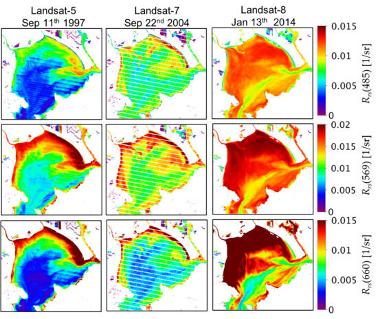
Two examples of products processed via SeaDAS are illustrated in Figure 6 and Figure 7. The goal is to qualitatively demonstrate the TM and ETM+ products and visually compare them to those obtained from OLI. Note that these products are associated with different seasons/times; therefore, this analysis is not suitable to gauge consistency, which will be discussed in Section 3.2.2 and Section 3.3. Note that a -element (uniform) averaging filter is applied in the aerosol removal process. Figure 6 illustrates the products derived from TM (left), ETM+ (middle), and OLI (right) over the turbid and shallow northern San Francisco Bay area (i.e., San Pablo Bay). The natural variability (e.g., gradients in optical regimes) in water-column is clearly captured in TM and ETM+ images. Small eddies, local resuspensions, and upwelling events can visually be discerned in the TM- and ETM+-derived products. Nevertheless, artifacts are pronounced in TM and ETM+ products when compared to those of OLI. The artifacts in TM products (in particular in the blue band) are due to memory effect, coherent noise, and striping [13]. Due to OLI’s higher SNR and absence of major artifacts, the quality of OLI products is noticeably better than those of TM and ETM+. The scan-line corrector issue, i.e., SLC-off, [3] associated with ETM+ retrievals are masked, i.e., white stripes. Furthermore, it should be noted that, although TM and ETM+ measure spectral radiances in three broad bands, these bands capture relatively distinct spectral signatures of near-surface constituents and their optical properties.
Another demonstration of the natural variability in inland and nearshore coastal waters captured in Rrs(569) and Rrs(560) products derived from TM and ETM+ is illustrated in Figure 7. The images were acquired eight days apart in September 2006 over the eastern North Carolina inland waters and shorelines. The scan-line corrector issues (i.e., SLC-off) associated with ETM+ retrievals are masked (shown with white stripes). The TM and ETM+ clearly reveal various water types, such as relatively clear waters in the coastal shelf area, nearshore turbid waters, and CDOM-rich river waters denoted with arrows, i.e., Tar/Pamlico River. Resuspension events can also be inferred in shallower waters. These demonstrations suggest the remarkable value of archived Landsat data and their utility enabled via SeaDAS. The negative retrievals, i.e., failure of the atmospheric correction, in CDOM-rich river waters are a known problem requiring further study and investigations into the future.
3.2. Validation
For a quantitative assessment of heritage Landsat products, we utilized two data sources; (a) AERONET-OC data and (b) Rrs products obtained from MODIS. This was to provide as much evidence as possible to ensure that these products were, on average, in reasonable agreement with standard products.
3.2.1. AERONET-OC
Since the early 2000s, the AERONET-OC data (https://aeronet.gsfc.nasa.gov) have been used as standard datasets to evaluate the quality of ocean color data products. Although the sites do not represent global in-water conditions, they provide adequate and easily accessible matchups to evaluate the performance of both atmospheric correction and instrument’s radiometric characteristics. The scatterplots for ETM+ and TM data for all the bands are shown in Figure 8. For the matchups, hazy images and areas affected by partial sunglint were removed from the analyses. A total of 216 and 79 matchups were found for ETM+ and TM data, respectively. For TM and ETM+, >90% and >65% of the matchups correspond to moderately turbid waters of the Venise (located in Northern Adriatic Sea) and Martha’s Vineyard (situated in southern coastal waters of Massachusetts) sites. The statistics were generated in a similar fashion as in Equations (3)–(5).
The computed statistics after implementing gains (Table 3) are provided in Table 4. For reference, MRD and root-mean-square error (RMSE) computed with unity gains, i.e., prior to implementing the gains, are given in round brackets. Note that RMSE was computed as in Equation (3); yet, here, we treat the AERONET-OC data as reference standards. Comparing MRD and RMSE statistics indicate that the vicarious gains, on average, have significantly reduced median biases in products (in particular for TM); thereby enhancing the overall consistency in long-term Landsat-derived products. The slope and intercepts for TM matchups allude to potential non-linearity at low radiance levels. Collectively, the statistics suggest that TM products should be handled with care when accurate/precise products (e.g., Chl) are desired. The best performances are, in general, found in the green channels. The relatively large slopes in ETM+ analyses implicate potential nonlinearity in instrument responses. We further computed the median spectra, i.e., , from AERONET-OC data to estimate percent RMSE () in retrievals. The for ETM+ and TM data were 0.0049, 0.00519, 0.00146 [1/sr] and 0.0050, 0.00371, 0.0013 [1/sr], respectively. The percent RMSEs were estimated as 36%, 28%, 62%, and 46%, 35%, 84% for ETM+ and TM’s blue, green, and red bands, respectively. Although the quality of ETM+ are adequately evaluated here using AERONET-OC data, there is still a need to better assess TM products over a broader range of water bodies.
3.2.2. MODIS-Derived Rrs Products
Since the AERONET-OC data do not provide a full representation of aquatic conditions in inland and nearshore coastal waters, we further evaluated TM/ETM+ products against (same-day) MODISA and MODIST products over the central basin of Lake Mead (n = 100/101), San Francisco (SF) Bay (n = 63/75), San Pablo Bay (n = 66/69), and the eastern basin of Lake Erie (n = 19/29) in North America for which a rich archive of TM data is available (limitations in the data downlink during periods of TM operations preclude a robust global analysis). The number of matchups (in round brackets) refer to the number of MODIST-ETM+ and MODISA-TM matchups, respectively. These sites collectively enable a fair assessment of TM and ETM+ products over a wider range of aquatic conditions (e.g., areas with high CDOM and/or sediment loads) and are sufficiently spatially extensive for valid ocean color products from MODIS observations.
Landsat-5, Landsat-7, and Terra were/are all morning satellites, while Aqua is in an afternoon orbit. Our initial assessments indicated noticeable uncertainties in intercomparisons due to the large time differences between ETM+ and MODISA overpasses. This was, in particular, observed over SF Bay influenced by significant tidal forcing. Therefore, for cross-validating ETM+ products, MODIST products were applied. In addition, because the two missions are in very similar orbits, near-nadir MODIST observations/products are available for cross-validating ETM+ products. On the other hand, Landsat-5 and Terra’s orbits are different such that only MODIST observations at the edge of the swaths are available for valid, same-day intercomparisons with those of TM. Such products are represented with large footprint sizes; therefore, larger uncertainties in products are expected. It was then decided to utilize MODISA products for investigating TM products, recognizing that there is two-to-three-hour time gap between data collections, which increase uncertainties in intercomparisons. The Level-1B MODIS data were processed to Level-2 products using a NIR-SWIR band combination [73]. The rest of the parameter-setting was identical to the current NASA Ocean Biology Processing Group’s standard processing. The spatial sampling for Aqua-MODIS products were conducted by taking the median values within 33-element windows to avoid contaminations from land. The equivalent sample area for Landsat products (i.e., median within 3 3 km regions) were adjusted according to MODIS viewing geometries. Further, the differences in the spectral bands were accounted for [61]. Figure 9 shows the scatterplots with the statistical analyses tabulated in Table 5.
Overall, there is a reasonable correlation in MODIST-ETM+ intercomparisons. The scattered matchups correspond to artifacts in TM and ETM+ products, uncertainties in the atmospheric correction, the spectral band adjustments, and possible changes in water-column conditions (in particular for TM-MODISA intercomparisons over SF Bay and San Pablo Bay influenced by strong tides). The uncertainties due to the time difference in overpasses were also found over Lake Mead and Lake Erie when both MODIST-ETM+ and MODISA-ETM+ intercomparisons were examined. Further site-specific analyses suggested larger uncertainties in TM-derived blue and red bands in Lake Mead and Lake Erie where Rrs(485) and Rrs(660) were, on average, 0.0034 [1/sr] and 0.0022 [1/sr], respectively.
3.3. Time-Series Applications
In order to examine the long-term record of Landsat-derived products, we analyzed seasonal composites generated for 12 aquatic systems across the continental USA. The seasonal composite plots were derived from locally processed Landsat data over 12 sites, three of which are presented in this manuscript. The median computed in each season represents seasonal composite products, which were produced to minimize noise in the analyses. The three plots shown in Figure 10, Figure 11 and Figure 12 correspond to the Indian River Lagoon (IRL) (27.8355N, 80.4515W), Pamlico Sound (35.1963N, 76.2670W), and San Joaquin River (38.09182N, 121.6297W). The other sites were Boston Harbor (MA), Suisan Bay (CA), Neuse River (NC), Upper Chesapeake Bay (MD), Potomac River (MD), San Francisco Bay (CA), Onondaga Lake (NY), Lake Tahoe (CA), and Crater Lake. The only products evaluated were for the three visible bands (Table 1). Figure 10 shows these products for the IRL in the vicinity of Sebastian Inlet State Park (FL).
Our approach developed for compensating for non-zero Lw(NIR) (Section 2.1) significantly increased the number of valid retrievals, i.e., more than 40% of the retrievals were negative in Rrs(485) products. Since data were collected eight days apart, potentially yielding biases in seasonal composites, it is difficult to infer consistency in the data products. In addition, seawater-intrusion and tidal exchanges may complicate such analyses. Seasonal composites over Pamlico Sound, North Carolina, are illustrated in Figure 11. Some of the retrievals may be associated with the noise in the NIR and SWIR-I bands that propagate through the atmospheric correction [64]. Note that prior to accounting for Lw(NIR) the entire record in the blue band was invalid. The time-series plot for the San Joaquin River (California) is shown in Figure 12 For this riverine system dominated with scattering particles, Lw(NIR) should be accounted for to allow for valid and/or accurate retrievals [54]. Similar results were found for a downstream system, i.e., Suisan Bay. The impact of the proposed methodology was most noticeable in such CDOM-dominated waters, i.e., frequent negative retrievals in the blue and green were observed prior to its implementation.
4. Discussions: Product Quality
The analyses thus far have highlighted some of the potentials and limitations of Landsat archive for long-term aquatic science studies. Now, with a rigorous, physics-based processing system in place, the science community can further explore the utility of the Landsat data record in science studies, such as examining impacts of human-induced activities (e.g., landuse/landcover change) on water quality. We demonstrated that following the cross-calibration and vicarious calibration of TM and ETM+ data, the biases in Rrs products are significantly reduced. In this section, we will further elaborate on the limitations of TM and ETM+ Rrs products with regard to noise contributions and processing flaws. A brief discussion on adjacency effects is also provided.
4.1. Signal-to-Noise Ratio (SNR)
Although we showed that TM- and ETM+-derived Rrs products agree well, on average, with those of OLI [59], OLI’s SNR is three-to-four times higher than those of TM and ETM+ [5,12]. To better understand the implications of these differences in Rrs products, a brief sensitivity analysis is carried out. Here, a small subset () of a cloud-free OLI image (ID:LC80220402014227LGN00, solar zenith angle of ) with low aerosol load, i.e., AOT(865) = 0.08, and over moderately turbid waters (Table 6) was processed by introducing various noise levels to simulate TM, ETM+, and OLI performances [5,12]. For each sensor, noise () is estimated via . The median and (derived from OLI subset) are tabulated in Table 6. The SNRs are adopted from References [5,74].
Note that OLI’s SNR from [74] were scaled to match the SNRs derived from typical radiances reported in Reference [5] for TM, ETM+, and MODIS. The analyses were conducted via Monte Carlo simulations for all the bands (Table 1) except the SWIR-II band, which was not used in the aerosol removal. To provide a reference, the OLI subset was also processed with the MODIS noise performance [5] representing a high-fidelity ocean color sensor. To generate various scenarios, were allowed to vary within the range with having a normal distribution. All the permutations resulted in ~7000 SeaDAS runs, which were repeated four times for TM, ETM+, OLI, and MODIS.
The uncertainties () provided in Table 4 represent one standard deviation derived from the resultant Rrs distributions. The derived uncertainties provide guidance on expected random variability in heritage Landsat products compared to those derived from OLI and MODIS. In general, the uncertainties in TM are two-to-five times higher than those of OLI. Given the magnitude of the spectrum, uncertainties in TM-, ETM+-, OLI-, and MODIS-derived Rrs products are, on average, ~ 25%, ~27%, ~8%, and ~2%, in the blue and green bands, respectively. This implies that subtle changes in , i.e., < , leading to small changes in water quality parameters, may not be detected. In inland and nearshore coastal waters (e.g., bays, estuaries) where concentrations of TSS and Chl are often much higher than those in coastal ocean waters, highly precise concentrations (at levels expected from ocean color missions) may not be required. Therefore, end-users may utilize heritage Rrs products with the “fit-for-purpose” concept in mind, i.e., products could be valuable for one application but may not be viable for another.
In addition, the choice of algorithm may alter how the noise is propagated to end products. For example, band-ratio algorithms [75,76] amplify the uncertainties. It is, thus, critical that users apply smoothing techniques, i.e., spatial filtering, (available to users by default via SeaDAS) to reduce the uncertainties. Assuming a -element (uniform) averaging window, in Table 6 are reduced by a factor of 1/7. This analysis was carried out for TOA radiance. In practice, increases with increase in leading to variable uncertainties across a scene. Note, however, that the median considered in this analysis is higher than typical radiances encountered in Landsat scenes [74]. Hence, the computed values in Table 6 provide an upper bound for (random component of) uncertainties.
It should also be noted that although ETM+’s SNRs in the visible bands are higher than those of TM, uncertainties in TM-derived are slightly smaller. This is attributed to TM’s higher SNR in the NIR band employed in the aerosol removal [64].
4.2. Image Artifacts and Processing Flaws
Heritage Landsat data, in particular TM images, often contain artifacts (e.g., striping, coherent noise, memory effects) suggesting that products should always be interpreted with care. Some of these artifacts are evident in Figure 6. Further, we found anomalies in TM products within the 1990–94 interval. This is highlighted in Figure 13 where time-series of products over fairly optically stable inland waters [59], i.e., Crater Lake and Lake Tahoe, are illustrated. Further analyses of and other intermediate products (e.g., ) indicated unusually high in the red, NIR, and SWIR-I bands. These high radiometric responses yield invalid products [64]. No such anomalies were identified for ETM+ time-series, i.e., fewer artifacts present in ETM+ data. Nonetheless, occasional noisy retrievals were observed in time-series plots. Another observation was nonlinearity in response when adjusting vicarious gains in Section 2.3. This was, in particular, confirmed in the ETM+ matchup analysis (Table 5). Overall, the products may be used with caution in oligotrophic (e.g., Crater Lake), mesotrophic (e.g., Lake Tahoe), and CDOM-rich waters.
To infer uncertainties in products, we quadratically added up systematic and random errors. It is, in general, difficult to fully characterize systematic errors for heritage sensors/products. However, according to the matchup analyses (Table 4), intercomparisons with MODIS (Table 5), and SNR assessments (Table 6), it is possible to speculate a maximum uncertainty estimate of 0.0019, 0.0018, and 0.0012 [1/sr] in the blue, green, and red channels of TM and ETM+ products, respectively. These estimates are calculated by taking the average of RMSEs in Table 4 and Table 5. Also, note that these maximum uncertainties are estimated recognizing (a) implementation of smoothing filters for reducing random noise contribution and (b) uncertainties in the matchup/intercomparison analyses. The changes and/or anomalies larger than the above threshold are expected to be detected in the heritage products. According to the matchup analyses (Section 3.2), the quality of the TM-derived Rrs(660) were found to be reliable for relatively highly backscattering waters where Rrs(660) > 0.004 [1/sr]. Our processing system may also contribute to uncertainties. For instance, it is likely that the retrievals over Crater and Tahoe lakes are affected by imperfect corrections of water-vapor transmission. Bear in mind that TM and ETM+’s NIR channels (Figure 1), i.e., ~140 nm wide, contain a water absorption feature centered around ~820 nm, whereas OLI’s NIR band is relatively narrow (Figure 1). Furthermore, some of the existing noise in the analyses may be attributed to failure in cloud-screening/-masking conducted using thresholds adopted from ocean color data processing. There are also inaccurate retrievals in periods where CDOM loads are high leading to the underestimation of Rrs. More research must be dedicated to these topics to enhance these historic Rrs products.
4.3. Adjacency Effects
The adjacency effect (AE) is another prime topic when using Landsat data in inland waters. Such signal complicating retrievals were pronounced over Onondaga Lake (NY). To qualitatively evaluate presence/absence of adjacency effects, the Rayleigh-corrected () data over three sites, including Onondaga Lake (NY), Chowan River (NC), and Boston Harbor (MA) were analyzed. The exact locations for these sites are (43.0919N, 76.2145W), (36.1763N, 76.7378W), and (42.3401, 70.9824W), respectively. To do so, below index () was computed
Although (ranging from −1 to 1) includes aerosol contributions, it provides insights into whether the spectrum deviates from expected trends, i.e., a monotonically decreasing one towards longer wavelengths. Therefore, the higher the , the stronger the NIR signal is, potentially alluding to the presence of adjacency effects. The time-series plots of extracted from Boston Harbor, Chowan River, and Onondaga Lake are illustrated in Figure 14. From the analyses of the Rrs data products (not shown here) over the Boston Harbor and the corresponding time-series shown in Figure 14, it appears that there is negligible adjacency effect. Considering the plots associated with Boston Harbor as the reference, it is found that there is AE in some instances of Chowan River retrievals. The impact of AE is much more pronounced over Onondaga Lake where is frequently very close to zero and even positive for some instances. Since the topography around Onondaga Lake and Chowan River is fairly flat and the two systems are comparable in their morphology, i.e., <2 km wide, it can be concluded that environmental conditions (e.g., wind, humidity, turbulence at land-atmosphere interface) play a major role in the magnitude of adjacency signal.
While with only six spectral measurements of TM and ETM+, it is nearly impossible to remove adjacency effects, it is certainly possible to minimize such effects with prior knowledge of the spectral characteristics of surrounding land targets, dominant environmental conditions and topography. Therefore, it is cautioned that the adjacency signals may not be assumed for all inland water sites (simply because they are small or narrow water bodies). For instance, land signals were not identified over San Joaquin River (CA), which is narrower than Onondaga Lake or Chowan River. Extensive research is required to identify water bodies susceptible to these effects, understand the dominant environmental conditions, and minimize them for the past and existing multispectral missions. With future hyperspectral missions planned/proposed for the next decade, it may be possible to more accurately account for these unwanted signals. Note further that the increased in the 1992–1996 period (marked with ovals) verifies a potential issue in TM products (as in Figure 13), which requires further investigation. Since products are not corrected for aerosol contributions, irregularities in Landsat-5 orbit may explain such anomalous trends in time-series analyses that do not accounted for variations in solar angles/radiation [77].
5. Conclusions
This work described the potentials and limitations of heritage Landsat missions for use in aquatic studies. Here, we demonstrated that the Landsat-5 and Landsat-7 data records, when corrected for atmospheric effects and vicariously calibrated via the algorithms and software available in the SeaWiFS Data Analysis System (SeaDAS), yield remote-sensing reflectance () products that, on average, agree with those derived from in situ measurements and/or other ocean color products. We further proposed a slightly different strategy to account for Lw(NIR) for TM and ETM+, which were/are missing the 443 nm channel. With careful regional or global algorithm developments, the processing system has enabled the creation of a long-term record of aquatic science products since 1984. Nevertheless, larger uncertainties in TM and ETM+ due to random and systematic noise, along with the availability of only three visible spectral bands, limit the choice of algorithms. Hence, algorithm developments for estimating turbidity and concentrations of TSS may be conducted with care. Following our analyses of several water bodies in North America, the TM and ETM+ data products are recommended to be developed and used in moderately to highly turbid waters (i.e., Rrs(660) > 0.004 [1/sr]), where instrument artifacts are less noticeable. Overall, although the uncertainties in TM and ETM+ products are higher than those of OLI, they are still valuable assets for retrospective studies. This may include assessing changes in water quality of lakes, reservoirs, water supplies, and coastal receiving waters due to short-/long-term landuse/landcover changes as well as examining climate variability (i.e., weather patterns) and its impacts on water quality (e.g., location, frequency, and persistence in historic harmful algal blooms). There is also a need for the community to measure and quantify optical properties of water constituents in these poorly known aquatic systems. A more extensive database of in-water optical properties will enable developing regional or global long-term aquatic science products. Future research should focus on (a) developing algorithms that are less prone to random noise, (b) enhancing atmospheric correction to account for non-negligible near-infrared reflectance in extremely turbid or CDOM-rich waters, and (c) characterizing adjacency effects under various environmental/climatic conditions.
Author Contributions
The analyses were all performed by S.V.B., N.P. led and wrote the manuscript, B.A.F. provided the necessary look-up-tables, and S.S. integrated the processing in SeaDAS.
Funding
Nima Pahlevan has been funded under NASA ROSES #NNX16AI16G, USGS Landsat Science Team Award #140G0118C0011, and the Massachusetts Institute of Technology SeaGrant Award # 2015-R/RC-140.
Acknowledgments
The authors are sincerely grateful to Wesley Moses for his comments and commitment to enhancing the quality of this manuscript. The reviewers’ efforts which helped enrich the discussions on product uncertainties are appreciated as well. We also would like to thank Landsat-8 project scientist Jim Irons, with NASA Goddard Space Flight Center, for his encouragements and support of this study. The authors also thank the MOBY Operations Team and the BOUSSOLE project for maintaining and disseminating in situ radiometric data. We also thank three anonymous reviewers for their very constructive comments.
Conflicts of Interest
The authors declare no conflicts of interest.
References
- Williams, D.L.; Goward, S.; Arvidson, T. Landsat. Photogramm. Eng. Remote Sens. 2006, 72, 1171–1178. [Google Scholar] [CrossRef]
- Markham, B.L.; Storey, J.C.; Williams, D.L.; Irons, J.R. Landsat sensor performance: History and current status. IEEE Trans. Geosci. Remote Sens. 2004, 42, 2691–2694. [Google Scholar] [CrossRef]
- Schott, J.R. Remote Sensing the Image Chain Approach, 2nd ed.; Oxford University Press: New York, NY, USA, 2007; p. 666. [Google Scholar]
- Gerace, A.D.; Schott, J.R.; Nevins, R. Increased potential to monitor water quality in the near-shore environment with Landsat’s next-generation satellite. J. Appl. Remote Sens. 2013, 7, 073558. [Google Scholar] [CrossRef]
- Hu, C.; Feng, L.; Lee, Z.; Davis, C.O.; Mannino, A.; McClain, C.R.; Franz, B.A. Dynamic range and sensitivity requirements of satellite ocean color sensors: Learning from the past. Appl. Opt. 2012, 51, 6045–6062. [Google Scholar] [CrossRef] [PubMed]
- Helder, D.L.; Markham, B.L.; Thome, K.J.; Barsi, J.A.; Chander, G.; Malla, R. Updated Radiometric Calibration for the Landsat-5 Thematic Mapper Reflective Bands. IEEE Trans. Geosci. Remote Sens. 2008, 46, 3309–3325. [Google Scholar] [CrossRef]
- Markham, B.; Goward, S.; Arvidson, T.; Barsi, J.; Scaramuzza, P. Landsat-7 long-term acquisition plan radiometry-evolution over time. Photogramm. Eng. Remote Sens. 2006, 72, 1129–1135. [Google Scholar] [CrossRef]
- Markham, B.L.; Boncyk, W.C.; Helder, D.L.; Barker, J.L. Landsat-7 Enhanced Thematic Mapper Plus Radiometric Calibration. Can. J. Remote Sens. 1997, 23, 318–332. [Google Scholar] [CrossRef]
- Barnes, B.B.; Hu, C.; Holekamp, K.L.; Blonski, S.; Spiering, B.A.; Palandro, D.; Lapointe, B. Use of Landsat data to track historical water quality changes in Florida Keys marine environments. Remote Sens. Environ. 2014, 140, 485–496. [Google Scholar] [CrossRef]
- IOCCG. Status and Plans for Satellite Ocean-Colour Missions: Considerations for Complementary Missions; Yoder, J.A., Ed.; IOCCG: Dartmouth, NS, Canada, 1999. [Google Scholar]
- IOCCG. Remote Sensing of Ocean Colour in Coastal, and Other Optically-Complex, Waters; Sathyendranath, S., Ed.; Reports of the International Ocean-Colour Coordinating Group (IOCCG); IOCCG: Dartmouth, NS, Canada, 2000. [Google Scholar]
- Pahlevan, N.; Schott, J. Leveraging EO-1 to Evaluate Capability of New Generation of Landsat Sensors for Coastal/Inland Water Studies. IEEE J. Sel. Top. Appl. Earth Obs. Remote Sens. 2013, 6, 360–374. [Google Scholar] [CrossRef]
- Helder, D.L.; Ruggles, T.A. Landsat thematic mapper reflective-band radiometric artifacts. IEEE Trans. Geosci. Remote Sens. 2004, 42, 2704–2716. [Google Scholar] [CrossRef]
- Ouillon, S.; Douillet, P.; Andréfouët, S. Coupling satellite data with in situ measurements and numerical modeling to study fine suspended-sediment transport: A study for the lagoon of New Caledonia. Coral Reef. 2004, 23, 109–122. [Google Scholar]
- Doxaran, D.; Froidefond, J.M.; Castaing, P. Remote-sensing reflectance of turbid sediment-dominated waters. Reduction of sediment type variations and changing illumination conditions effects by use of reflectance ratios. Appl. Opt. 2003, 42, 2623–2634. [Google Scholar] [PubMed]
- Doxaran, D.; Froidefond, J.M.; Castaing, P.; Babin, M. Dynamics of the turbidity maximum zone in a macrotidal estuary (the Gironde, France): Observations from field and MODIS satellite data. Estuar. Coast. Shelf Sci. 2009, 81, 321–332. [Google Scholar] [CrossRef]
- Dekker, A.G.; Vos, R.J.; Peters, S.W.M. Comparison of remote sensing data, model results and in situ data for total suspended matter (TSM) in the southern Frisian lakes. Sci. Total Environ. 2001, 268, 197–214. [Google Scholar] [CrossRef]
- Baban, S.M. Detecting water quality parameters in the Norfolk Broads, UK, using Landsat imagery. Int. J. Remote Sens. 1993, 14, 1247–1267. [Google Scholar] [CrossRef]
- Ritchie, J.C.; Cooper, C.M.; Schiebe, F.R. The relationship of MSS and TM digital data with suspended sediments, chlorophyll, and temperature in Moon Lake, Mississippi. Remote Sens. Environ. 1990, 33, 137–148. [Google Scholar] [CrossRef]
- Mertes, L.A.; Smith, M.O.; Adams, J.B. Estimating suspended sediment concentrations in surface waters of the Amazon River wetlands from Landsat images. Remote Sens. Environ. 1993, 43, 281–301. [Google Scholar] [CrossRef]
- Bourgoin, L.M.; Bonnet, M.P.; Martinez, J.M.; Kosuth, P.; Cochonneau, G.; Moreira-Turcq, P.; Guyot, J.L.; Vauchel, P.; Filizola, N.; Seyler, P. Temporal dynamics of water and sediment exchanges between the Curuaí floodplain and the Amazon River, Brazil. J. Hydrol. 2007, 335, 140–156. [Google Scholar] [CrossRef]
- Stumpf, R.P.; Goldschmidt, P.M. Remote sensing of suspended sediment discharge into the western Gulf of Maine during the April 1987 100-year flood. J. Coast. Res. 1992, 8, 218–225. [Google Scholar]
- Dekker, A.G.; Vos, R.; Peters, S. Analytical algorithms for lake water TSM estimation for retrospective analyses of TM and SPOT sensor data. Int. J. Remote Sens. 2002, 23, 15–35. [Google Scholar] [CrossRef]
- Giardino, C.; Pepe, M.; Brivio, P.A.; Ghezzi, P.; Zilioli, E. Detecting chlorophyll, Secchi disk depth and surface temperature in a sub-alpine lake using Landsat imagery. Sci. Total Environ. 2001, 268, 19–29. [Google Scholar] [CrossRef]
- Allan, M.G.; Hamilton, D.P.; Hicks, B.J.; Brabyn, L. Landsat remote sensing of chlorophyll a concentrations in central North Island lakes of New Zealand. Int. J. Remote Sens. 2011, 32, 2037–2055. [Google Scholar] [CrossRef]
- Brezonik, P.; Menken, K.D.; Bauer, M. Landsat-based remote sensing of lake water quality characteristics, including chlorophyll and colored dissolved organic matter (CDOM). Lake Reserv. Manag. 2005, 21, 373–382. [Google Scholar] [CrossRef]
- Pattiaratchi, C.; Lavery, P.; Wyllie, A.; Hick, P. Estimates of water quality in coastal waters using multi-date Landsat Thematic Mapper data. Int. J. Remote Sens. 1994, 15, 1571–1584. [Google Scholar] [CrossRef]
- Kutser, T.; Pierson, D.C.; Kallio, K.Y.; Reinart, A.; Sobek, S. Mapping lake CDOM by satellite remote sensing. Remote Sens. Environ. 2005, 94, 535–540. [Google Scholar] [CrossRef]
- Nieke, B.; Reuter, R.; Heuermann, R.; Wang, H.; Babin, M.; Therriault, J. Light absorption and fluorescence properties of chromophoric dissolved organic matter (CDOM), in the St. Lawrence Estuary (Case 2 waters). Cont. Shelf Res. 1997, 17, 235–252. [Google Scholar] [CrossRef]
- Griffin, C.G.; Frey, K.E.; Rogan, J.; Holmes, R.M. Spatial and interannual variability of dissolved organic matter in the Kolyma River, East Siberia, observed using satellite imagery. J. Geophys. Res. Biogeosci. 2011, 116, G3. [Google Scholar] [CrossRef]
- Phinn, S.; Dekker, A.; Brando, V.E.; Roelfsema, C. Mapping water quality and substrate cover in optically complex coastal and reef waters: An integrated approach. Mar. Pollut. Bullet. 2005, 51, 459–469. [Google Scholar] [CrossRef] [PubMed]
- Armstrong, R.A. Remote sensing of submerged vegetation canopies for biomass estimation. Int. J. Remote Sens. 1993, 14, 621–627. [Google Scholar] [CrossRef]
- Lyzenga, D.R. Remote sensing of bottom reflectance and water attenuation parameters in shallow water using aircraft and Landsat data. Int. J. Remote Sens. 1981, 2, 71–82. [Google Scholar] [CrossRef]
- Andréfouët, S.; Muller-Karger, F.E.; Hochberg, E.J.; Hu, C.; Carder, K.L. Change detection in shallow coral reef environments using Landsat 7 ETM+ data. Remote Sens. Environ. 2001, 78, 150–162. [Google Scholar] [CrossRef]
- Capolsini, P.; Andréfouët, S.; Rion, C.; Payri, C. A comparison of Landsat ETM+, SPOT HRV, Ikonos, ASTER, and airborne MASTER data for coral reef habitat mapping in South Pacific islands. Can. J. Remote Sens. 2003, 29, 187–200. [Google Scholar] [CrossRef]
- Olmanson, L.G.; Bauer, M.E.; Brezonik, P.L. A 20-year Landsat water clarity census of Minnesota’s 10,000 lakes. Remote Sens. Environ. 2008, 112, 4086–4097. [Google Scholar] [CrossRef]
- Lavery, P.; Pattiaratchi, C.; Wyllie, A.; Hick, P. Water quality monitoring in estuarine waters using the Landsat Thematic Mapper. Remote Sens. Environ. 1993, 46, 268–280. [Google Scholar] [CrossRef]
- Tyler, A.; Svab, E.; Preston, T.; Présing, M.; Kovács, W. Remote sensing of the water quality of shallow lakes: A mixture modelling approach to quantifying phytoplankton in water characterized by high-suspended sediment. Int. J. Remote Sens. 2006, 27, 1521–1537. [Google Scholar] [CrossRef]
- Kutser, T. The possibility of using the Landsat image archive for monitoring long time trends in coloured dissolved organic matter concentration in lake waters. Remote Sens. Environ. 2012, 123, 334–338. [Google Scholar] [CrossRef]
- Lobo, F.L.; Costa, M.P.; Novo, E.M. Time-series analysis of Landsat-MSS/TM/OLI images over Amazonian waters impacted by gold mining activities. Remote Sens. Environ. 2015, 157, 170–184. [Google Scholar] [CrossRef]
- Lyons, M.B.; Roelfsema, C.M.; Phinn, S.R. Towards understanding temporal and spatial dynamics of seagrass landscapes using time-series remote sensing. Estuar. Coast. Shelf Sci. 2013, 120, 42–53. [Google Scholar] [CrossRef]
- Wang, Y.; Xia, H.; Fu, J.; Sheng, G. Water quality change in reservoirs of Shenzhen, China: Detection using LANDSAT/TM data. Sci. Total Environ. 2004, 328, 195–206. [Google Scholar] [CrossRef] [PubMed]
- Erkkilä, A.; Kalliola, R. Patterns and dynamics of coastal waters in multi-temporal satellite images: Support to water quality monitoring in the Archipelago Sea, Finland. Estuar. Coast. Shelf Sci. 2004, 60, 165–177. [Google Scholar] [CrossRef]
- Kallio, K.; Attila, J.; Härmä, P.; Koponen, S.; Pulliainen, J.; Hyytiäinen, U.-M.; Pyhälahti, T. Landsat ETM+ images in the estimation of seasonal lake water quality in boreal river basins. Environ. Manag. 2008, 42, 511–522. [Google Scholar] [CrossRef] [PubMed]
- Hui, F.; Xu, B.; Huang, H.; Yu, Q.; Gong, P. Modelling spatial-temporal change of Poyang Lake using multitemporal Landsat imagery. Int. J. Remote Sens. 2008, 29, 5767–5784. [Google Scholar] [CrossRef]
- Wulder, M.A.; Masek, J.G.; Cohen, W.B.; Loveland, T.R.; Woodcock, C.E. Opening the archive: How free data has enabled the science and monitoring promise of Landsat. Remote Sens. Environ. 2012, 122, 2–10. [Google Scholar] [CrossRef]
- Hu, C.; Muller-Karger, F.E.; Andrefouet, S.; Carder, K.L. Atmospheric correction and cross-calibration of LANDSAT-7/ETM+ imagery over aquatic environments: A multiplatform approach using SeaWiFS/MODIS. Remote Sens. Environ. 2001, 78, 99–107. [Google Scholar] [CrossRef]
- Antoine, D.; d’Ortenzio, F.; Hooker, S.B.; Bécu, G.; Gentili, B.; Tailliez, D.; Scott, A.J. Assessment of uncertainty in the ocean reflectance determined by three satellite ocean color sensors (MERIS, SeaWiFS and MODIS-A) at an offshore site in the Mediterranean Sea (BOUSSOLE project). J. Geophys. Res. Ocean. 2008, 113. [Google Scholar] [CrossRef] [Green Version]
- Hu, C.; Feng, L.; Lee, Z. Uncertainties of SeaWiFS and MODIS remote sensing reflectance: Implications from clear water measurements. Remote Sens. Environ. 2013, 133, 168–182. [Google Scholar] [CrossRef]
- IOCCG. Mission Requirements for Future Ocean-Colour Sensors; Reports of the International Ocean-Colour Coordinating Group; McClain, C.R., Meister, G., Eds.; IOCCG: Dartmuouth, NS, Canada, 2012; p. 102. [Google Scholar]
- Franz, B.A.; Bailey, S.W.; Kuring, N.; Werdell, P.J. Ocean color measurements with the Operational Land Imager on Landsat-8: Implementation and evaluation in SeaDAS. J. Appl. Remote Sens. 2015, 9, 096070. [Google Scholar] [CrossRef]
- Pahlevan, N.; Sarkar, S.; Franz, B.A.; Balasubramanian, S.V.; He, J. Sentinel-2 MultiSpectral Instrument (MSI) data processing for aquatic science applications: Demonstrations and validations. Remote Sens. Environ. 2017, 201, 47–56. [Google Scholar] [CrossRef]
- Siegel, D.A.; Wang, M.; Maritorena, S.; Robinson, W. Atmospheric correction of satellite ocean color imagery: The black pixel assumption. Appl. Opt. 2000, 39, 3582–3591. [Google Scholar] [CrossRef] [PubMed]
- Bailey, S.W.; Franz, B.A.; Werdell, P.J. Estimation of near-infrared water-leaving reflectance for satellite ocean color data processing. Opt. Express 2010, 18, 7521–7527. [Google Scholar] [CrossRef] [PubMed]
- Gordon, H.R. In-orbit calibration strategy for ocean color sensors. Remote Sens. Environ. 1998, 63, 265–278. [Google Scholar] [CrossRef]
- Franz, B.A.; Bailey, S.W.; Werdell, P.J.; McClain, C.R. Sensor-independent approach to the vicarious calibration of satellite ocean color radiometry. Appl. Opt. 2007, 46, 5068–5082. [Google Scholar] [CrossRef] [PubMed]
- Gordon, H.R.; Wang, M. Retrieval of water-leaving radiance and aerosol optical thickness over the oceans with SeaWiFS: A preliminary algorithm. Appl. Opt. 1994, 33, 443–452. [Google Scholar] [CrossRef] [PubMed]
- Ahmad, Z.; Franz, B.A.; McClain, C.R.; Kwiatkowska, E.J.; Werdell, J.; Shettle, E.P.; Holben, B.N. New aerosol models for the retrieval of aerosol optical thickness and normalized water-leaving radiances from the SeaWiFS and MODIS sensors over coastal regions and open oceans. Appl. Opt. 2010, 49, 5545–5560. [Google Scholar] [CrossRef] [PubMed]
- Pahlevan, N.; Schott, J.R.; Franz, B.A.; Zibordi, G.; Markham, B.; Bailey, S.; Schaaf, C.B.; Ondrusek, M.; Greb, S.; Strait, C.M. Landsat 8 remote sensing reflectance (Rrs) products: Evaluations, intercomparisons, and enhancements. Remote Sens. Environ. 2017, 190, 289–301. [Google Scholar] [CrossRef]
- Lee, Z.P.; Carder, K.L.; Arnone, R.A. Deriving inherent optical properties from water color: A multiband quasi-analytical algorithm for optically deep waters. Appl. Opt. 2002, 41, 5755–5772. [Google Scholar] [CrossRef] [PubMed]
- Pahlevan, N.; Smith, B.; Binding, C.; O’Donnell, D.M. Spectral band adjustments for remote sensing reflectance spectra in coastal/inland waters. Opt. Express 2017, 25, 28650–28667. [Google Scholar] [CrossRef]
- Clark, D.K.; Murphy, M.Y.; Yarbrough, M.; Feinholz, M.; Flora, S.; Broenkow, W.; Bettye, C.J.; Steven, W.B.; Kim, Y.S.; Mueller, J. MOBY, a radiometric buoy for performance monitoring and vicarious calibration of satellite ocean color sensors: Measurement and data analysis protocols. In Ocean Optics Protocols for Satellite Ocean Color Sensor Validation; Mueller, J.L., Giulietta, G.S., McClain, C.R., Eds.; NASA/NOAA/USAF: Greenbelt, MD, USA, 2003; p. 32. [Google Scholar]
- Antoine, D.; Guevel, P.; Deste, J.-F.; Bécu, G.; Louis, F.; Scott, A.J.; Bardey, P. The “BOUSSOLE” buoy-a new transparent-to-swell taut mooring dedicated to marine optics: Design, tests, and performance at sea. J. Atmos. Ocean. Technol. 2008, 25, 968–989. [Google Scholar] [CrossRef]
- Pahlevan, N.; Roger, J.-C.; Ahmad, Z. Revisiting short-wave-infrared (SWIR) bands for atmospheric correction in coastal waters. Opt. Express 2017, 25, 6015–6035. [Google Scholar] [CrossRef] [PubMed]
- Zibordi, G.; Mélin, F.; Berthon, J.-F.; Holben, B.; Slutsker, I.; Giles, D.; D’Alimonte, D.; Vandemark, D.; Feng, H.; Schuster, G. AERONET-OC: A network for the validation of ocean color primary products. J. Atmos. Ocean. Technol. 2009, 26, 1634–1651. [Google Scholar] [CrossRef]
- Bailey, S.W.; Hooker, S.B.; Antoine, D.; Franz, B.A.; Werdell, P.J. Sources and assumptions for the vicarious calibration of ocean color satellite observations. Appl. Opt. 2008, 47, 2035–2045. [Google Scholar] [CrossRef] [PubMed]
- Zibordi, G.; Mélin, F. An evaluation of marine regions relevant for ocean color system vicarious calibration. Remote Sens. Environ. 2017, 190, 122–136. [Google Scholar] [CrossRef] [PubMed]
- Franz, B.A.; Kwiatowska, E.J.; Meister, G.; McClain, C.R. Moderate Resolution Imaging Spectroradiometer on Terra: Limitations for ocean color applications. J. Appl. Remote Sens. 2008, 2, 023525. [Google Scholar] [CrossRef]
- Pahlevan, N.; Schott, J.R. Characterizing the relative calibration of Landsat-7 (ETM+) visible bands with Terra (MODIS) over clear waters: The implications for monitoring water resources. Remote Sens. Environ. 2012, 125, 167–180. [Google Scholar] [CrossRef]
- Uprety, S.; Cao, C.; Xiong, X.; Blonski, S.; Wu, A.; Shao, X. Radiometric intercomparison between Suomi-NPP VIIRS and Aqua MODIS reflective solar bands using simultaneous nadir overpass in the low latitudes. J. Atmos. Ocean. Technol. 2013, 30, 2720–2736. [Google Scholar] [CrossRef]
- Cao, C.; Weinreb, M.; Xu, H. Predicting Simultaneous Nadir Overpasses among Polar-Orbiting Meteorological Satellites for the Intersatellite Calibration of Radiometers. J. Atmos. Ocean. Technol. 2004, 21, 537–542. [Google Scholar] [CrossRef]
- Atmospheric Correction for Remotely-Sensed Ocean-Colour Products; Reports and Monographs of the International Ocean-Colour Coordinating Group (IOCCG); Wang, M. (Ed.) International Ocean-Colour Coordinating Group: Dartmouth, NS, Canada, 2010. [Google Scholar]
- Aurin, D.; Mannino, A.; Franz, B. Spatially resolving ocean color and sediment dispersion in river plumes, coastal systems, and continental shelf waters. Remote Sens. Environ. 2013, 137, 212–225. [Google Scholar] [CrossRef]
- Pahlevan, N.; Lee, Z.; Wei, J.; Schaff, C.; Schott, J.; Berk, A. On-orbit radiometric characterization of OLI (Landsat-8) for applications in aquatic remote sensing. Remote Sens. Environ. 2014, 154, 272–284. [Google Scholar] [CrossRef]
- Esaias, W.E.; Abbott, M.R.; Barton, I.; Brown, O.B.; Campbell, J.W.; Carder, K.L.; Clark, D.K.; Evans, R.H.; Hoge, F.E.; Gordon, H.R. An overview of MODIS capabilities for ocean science observations. IEEE Trans. Geosci. Remote Sens. 1998, 36, 1250–1265. [Google Scholar] [CrossRef] [Green Version]
- Carder, K.; Chen, F.R.; Lee, Z.; Hawes, S.K.; Cannizzaro, J.P. MODIS Ocean Science Team: Algorithm Theoretical Basis Document-ATBD19; College of Marine Science, University of South Florida: Tampa, FL, USA, 2003. [Google Scholar]
- Zhang, H.; Roy, D.P. Landsat 5 Thematic Mapper reflectance and NDVI 27-year time series inconsistencies due to satellite orbit change. Remote Sens. Environ. 2016, 186, 217–233. [Google Scholar]
Figure 1.
The relative spectral response (RSR) for the Thematic Mapper (TM), the Enhanced Thematic Mapper Plus (ETM+), and the Operational Land Imager (OLI) with their corresponding nominal center wavelength. The largest difference between TM/ETM+ and OLI is in the near infrared (NIR) channel where OLI band was designed narrow to avoid water-vapor absorption in the atmosphere.

Figure 2.
The strong relationship (left) between the band ratios of subsurface remote sensing reflectance in the blue and green channels, i.e., (482/561) and (443/561). The relationship follows the power-law function (A = 0.7554, B = 1.3994) and provides a high correlation coefficient, i.e., = 0.987. The scatterplot (right) shows the cross-validation of derived using two different band ratios, i.e., (443 /561) and (482/561).

Figure 3.
The vicarious gains (n = 58) for ETM+ visible bands. Each data point corresponds to a computed gain over the MOBY and/or BOUSSOLE site. The temporally median gains and (one) standard deviation applied to ETM+ data are provided in Table 2. Note that the gains are derived after vicariously calibrating NIR and SWIR-I bands in Step I.

Figure 4.
The vicarious gains for TM visible bands. Each data point corresponds to a TM-MODIS near-concurrent matchup, i.e., same-day overpasses, over various calibration sites. The temporally median gains and (one) standard deviation applied to TM data are provided in Table 2. Note that the gains are derived after vicariously calibrating NIR and SWIR-I bands.

Figure 5.
The scatterplots obtained from intercomparisons of OLI-ETM+ and TM-ETM+ Rrs products over optically stable waters of Crater and Tahoe lakes. The gains tabulated in Table 2 were supplied to SeaDAS to generate these products. Final gains are tabulated in Table 3. Note that the image pairs were acquired 8 days apart.

Figure 6.
The Rrs products derived from TM (left), ETM+ (middle), and OLI (right) over the northern San Francisco Bay area. The band centers shown to the right refer to TM bands. The scan-line corrector issues (i.e., SLC-off) associated with ETM+ retrievals are masked, i.e., white stripes. Varieties of physical phenomena, including upwelling events and sediment resuspensions are captured by heritage Landsat missions. Note that a -element (uniform) averaging filter is applied in the aerosol removal process.

Figure 7.
Scene-wide Rrs(569) and Rrs(560) products derived from TM (left) and ETM+ (right) over the North Carolina shorelines and Pamlico Sound (USA). The images were acquired eight days apart on 18 September (TM) and 26 September 2006 at about 15:30 GMT. Large gradients, i.e., relatively clear coastal shelf waters, eddies, resuspensions, CDOM-dominated waters and bottom features, are captured in the two images. The CDOM-rich waters of Tar/Pamlico Rivers are indicated with arrows. Note that negative retrievals do exist in such challenging waters in the ETM+ product [72] and a -element (uniform) averaging filter was applied in the aerosol removal process.

Figure 8.
The scatterplots for TM and ETM+ matchups at AERONET-OC sites. The low median biases (Table 4) indicate that the final vicarious gains, on average, have enhanced the overall consistency of Landsat-derived products. The matchups exclude retrievals in areas with partial glints. The AERONET-OC matchups (N = 216) enable a robust analysis of the ETM+ products, whereas the quality of TM products require further scrutiny (see Section 3.2.2).

Figure 9.
The scatterplots for the TM-MODISA and MODIST-ETM+ intercomparisons. Considering the dynamic range in the signal and the uncertainties in the intercomparisons, TM and ETM+ products are in good agreement with those of MODIS. The largest scatter is found in TM-derived Rrs(485) products. The larger uncertainties in the TM-MODISA analyses have aroused from two-to-three-hour time difference in their respective overpass times.

Figure 10.
The seasonal composites of Rrs products derived from Landsat-5 (solid circles), Landsat-7 (triangle), and Landsat-8 (hollow circles) over the Indian River Lagoon (27.8355N, 80.4515W), Florida. The composites were obtained by taking the median of retrievals in each season. The images were processed via SeaDAS. The methodology for accounting for non-negligible Lw(NIR) significantly improved the number of valid (non-negative) retrievals.

Figure 11.
Seasonal composites of Rrs products derived from Landsat-5 (solid circles), Landsat-7 (triangle), and Landsat-8 (hollow circles) in Pamlico Sound, North Carolina (35.1963N, 76.2670W). The composites were obtained by taking the median of retrievals in each season. The images processed via SeaDAS. The product consistency can be inferred in the overlapping periods indicating the utility of long-term Landsat data record for aquatic science studies. Note that because of the differences in the temporal sampling (i.e., eight days) and considering various tidal stages, a robust analysis of product consistency is not possible.

Figure 12.
Seasonal Rrs composites derived from Landsat-5 (solid circles), Landsat-7 (triangle), and Landsat-8 (hollow circles) in San Joaquin River (38.09182N, 121.6297W), California. The composites were obtained by taking the median of retrievals in each season. The images were processed via SeaDAS. The product consistency can be inferred in the cross-mission overlapping periods. Few negative retrievals are attributed to imperfect corrections for the contributing water-leaving radiance in the NIR channel.

Figure 13.
The time-series of Rrs products in the blue bands over optically stable waters of Crater and Tahoe lakes. The overall signal level is very similar in time. A potential anomaly found for TM products is highlighted in the Crater Lake time-series.
Figure 13.
The time-series of Rrs products in the blue bands over optically stable waters of Crater and Tahoe lakes. The overall signal level is very similar in time. A potential anomaly found for TM products is highlighted in the Crater Lake time-series.

Figure 14.
The AE_Ind computed for three sites to analyze presence/absence of adjacency effects (AE). The higher the index, the larger the magnitude of AE is. The Onondaga Lake has the highest and most frequent presence of AE whereas the effect is deemed to be negligible or absent over Boston Harbor. Note that the NIR bands of TM and ETM+ are much wider than that of OLI. This has likely resulted in smaller OLI-derived AE_Ind. The higher-than-normal AE_Ind highlighted with ovals may be due to abnormalities in Landsat-5 orbit in early/mid 90’s [77].


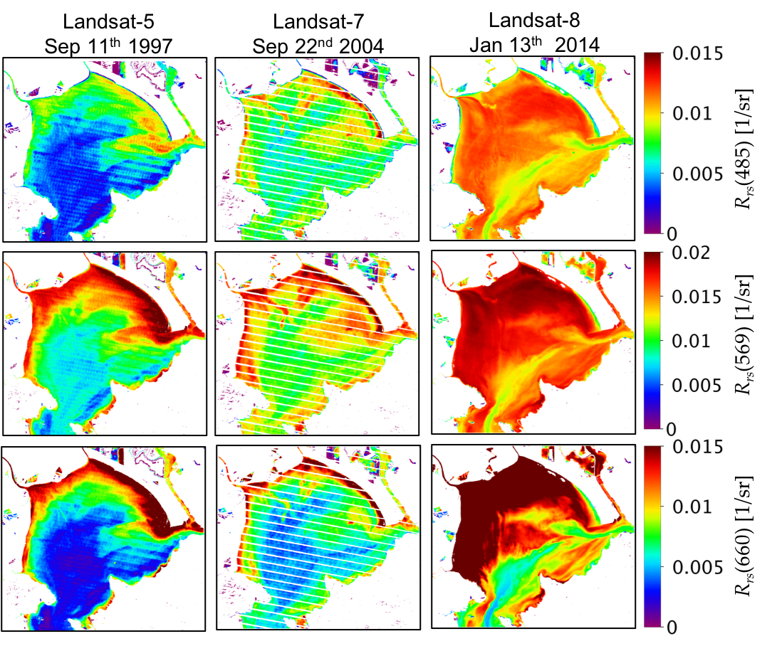
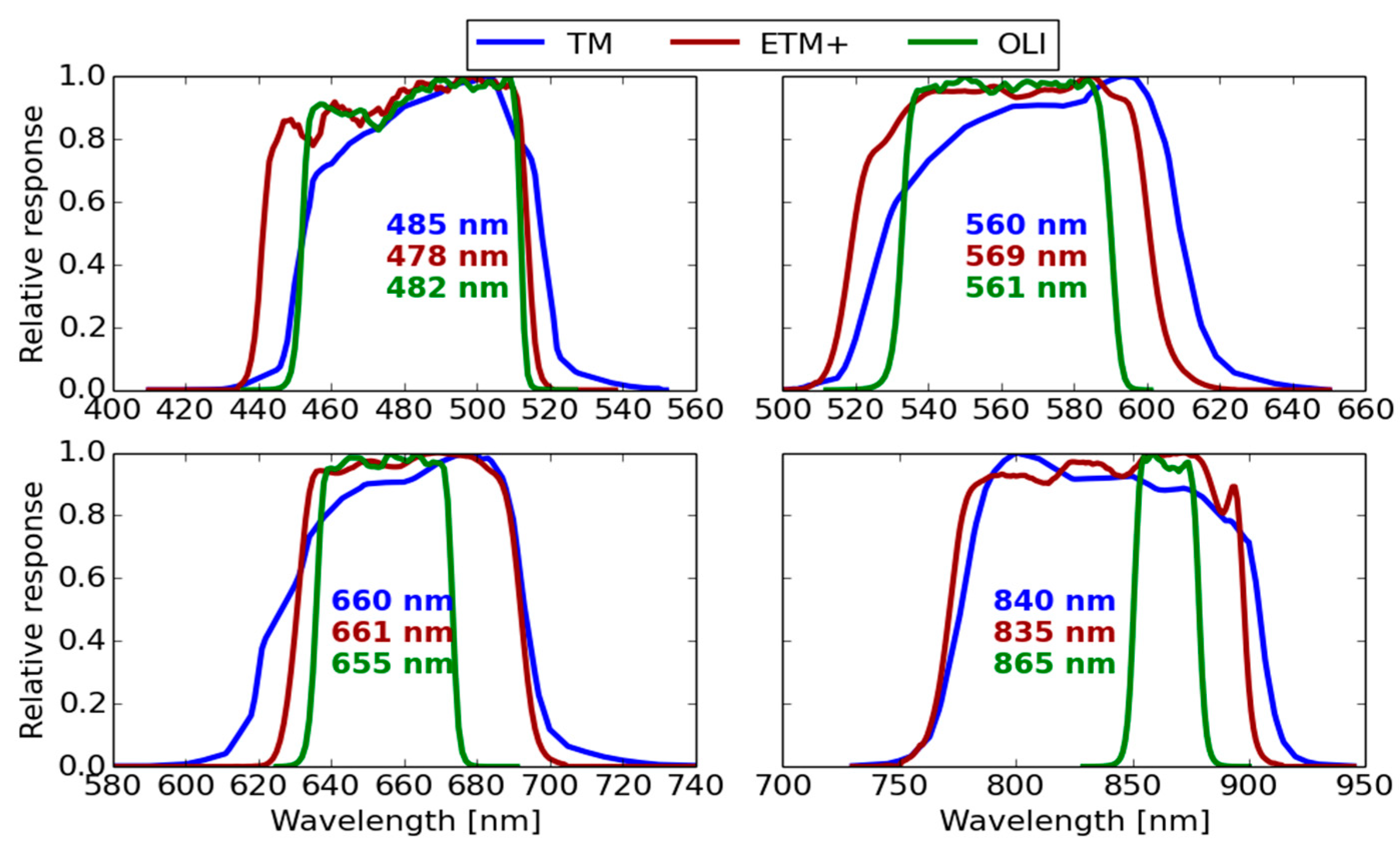
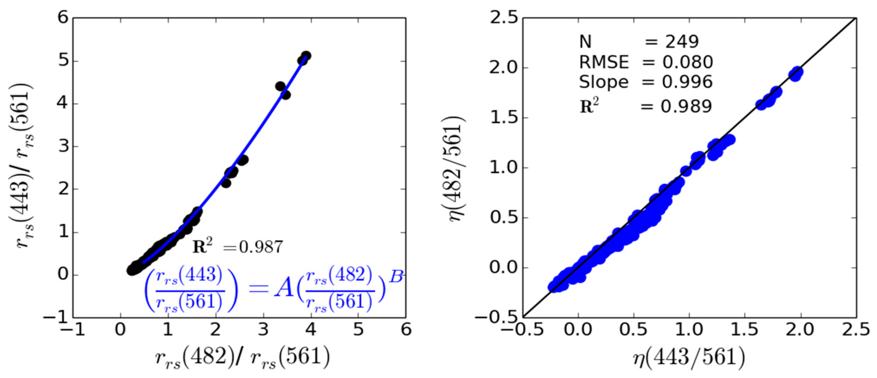
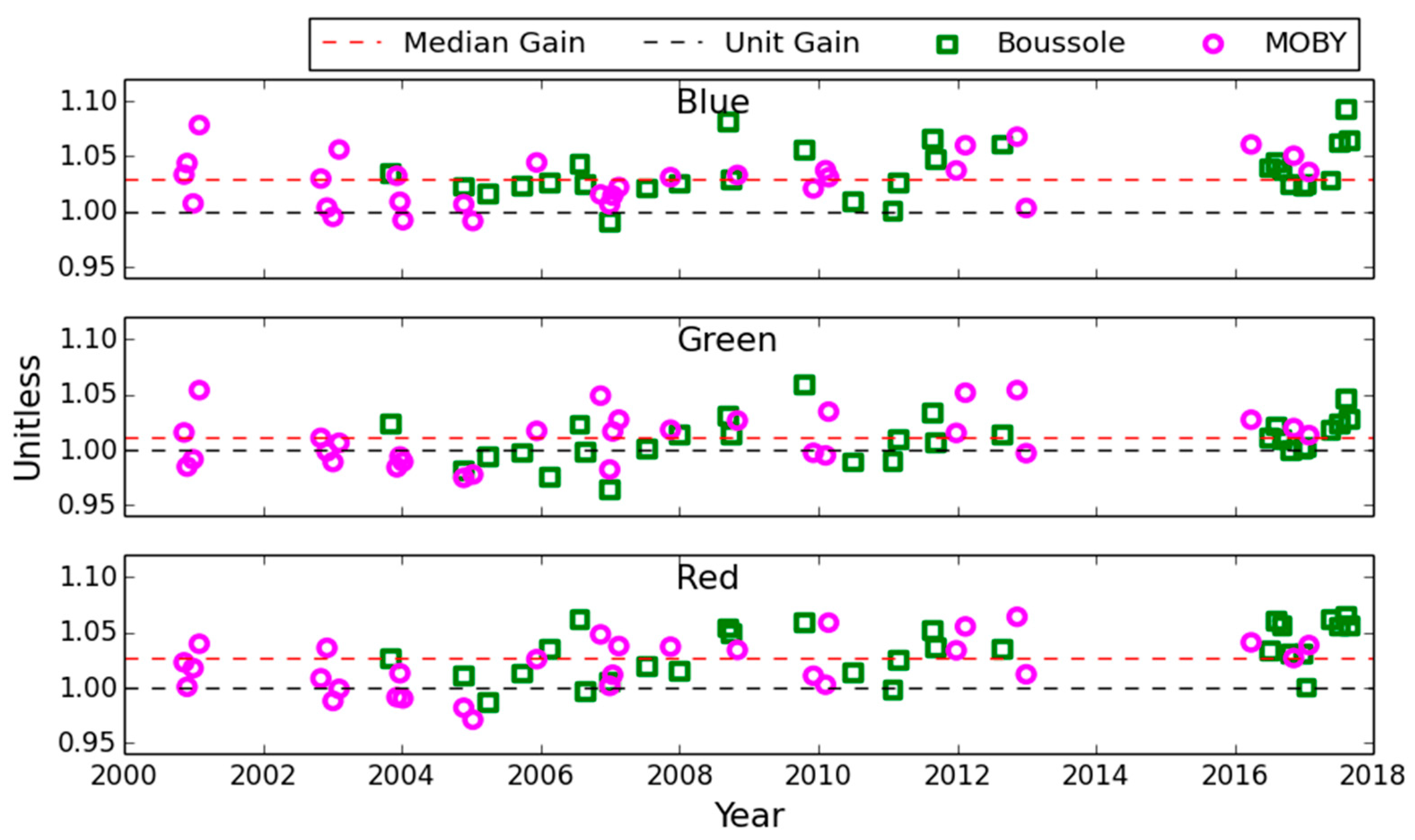
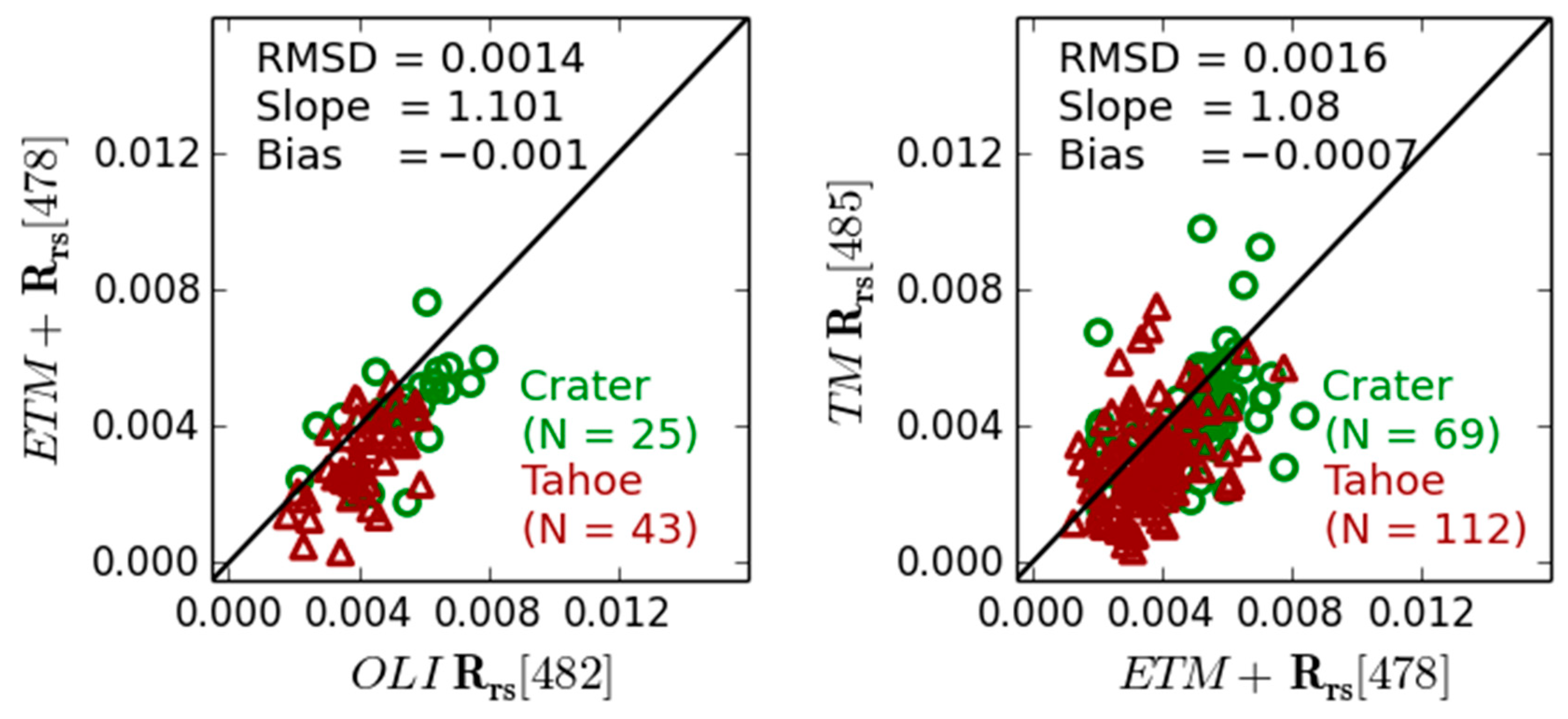
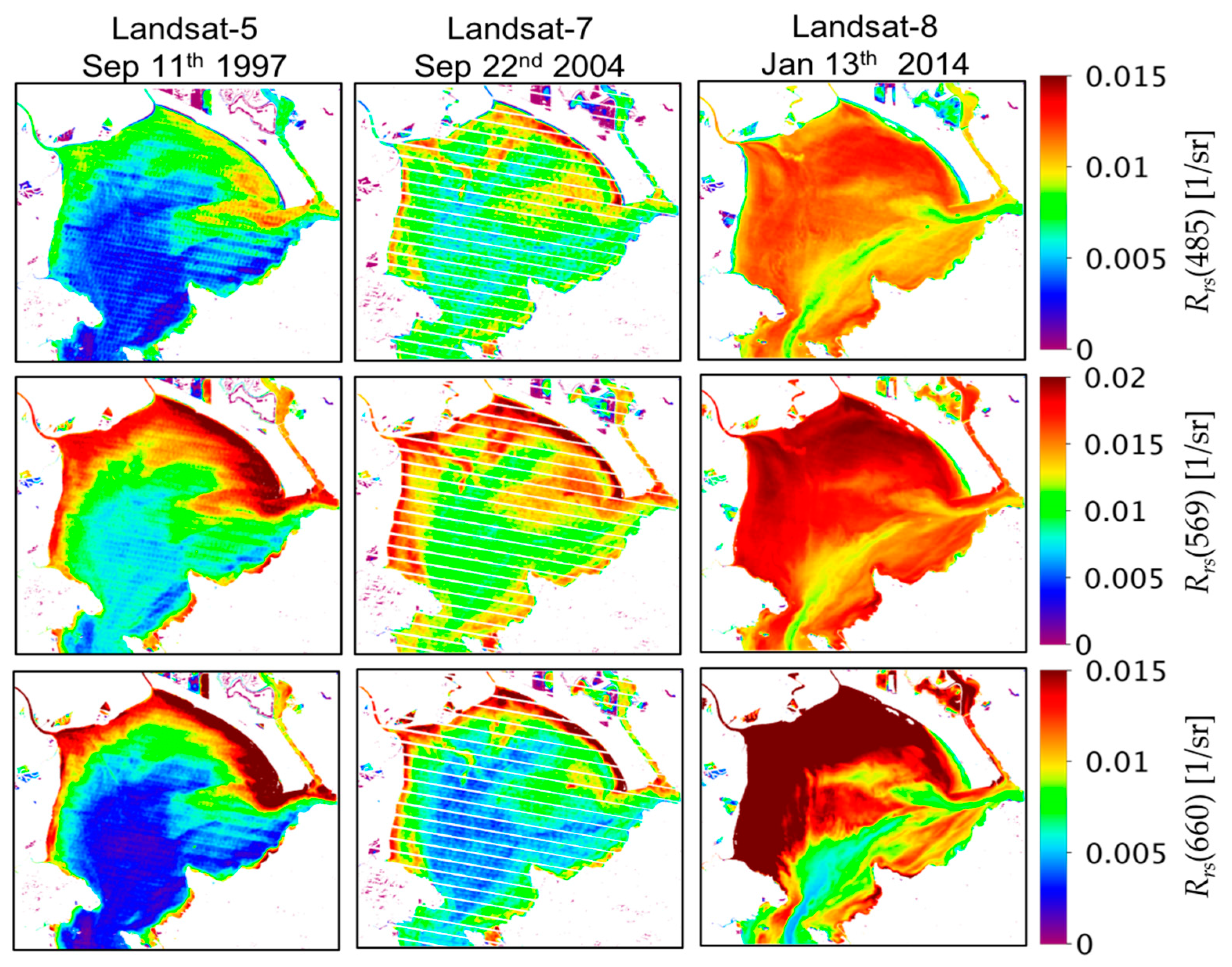
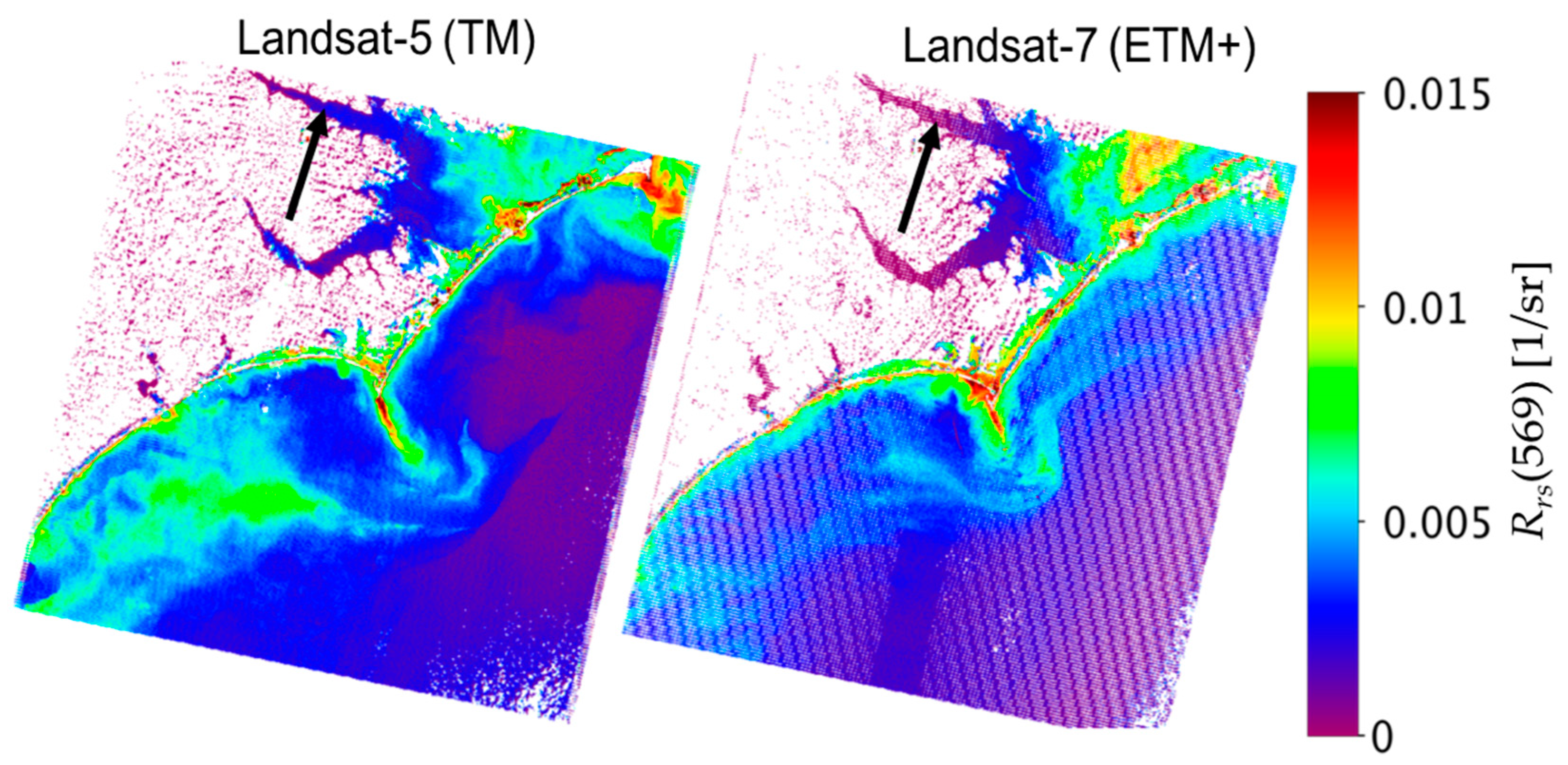
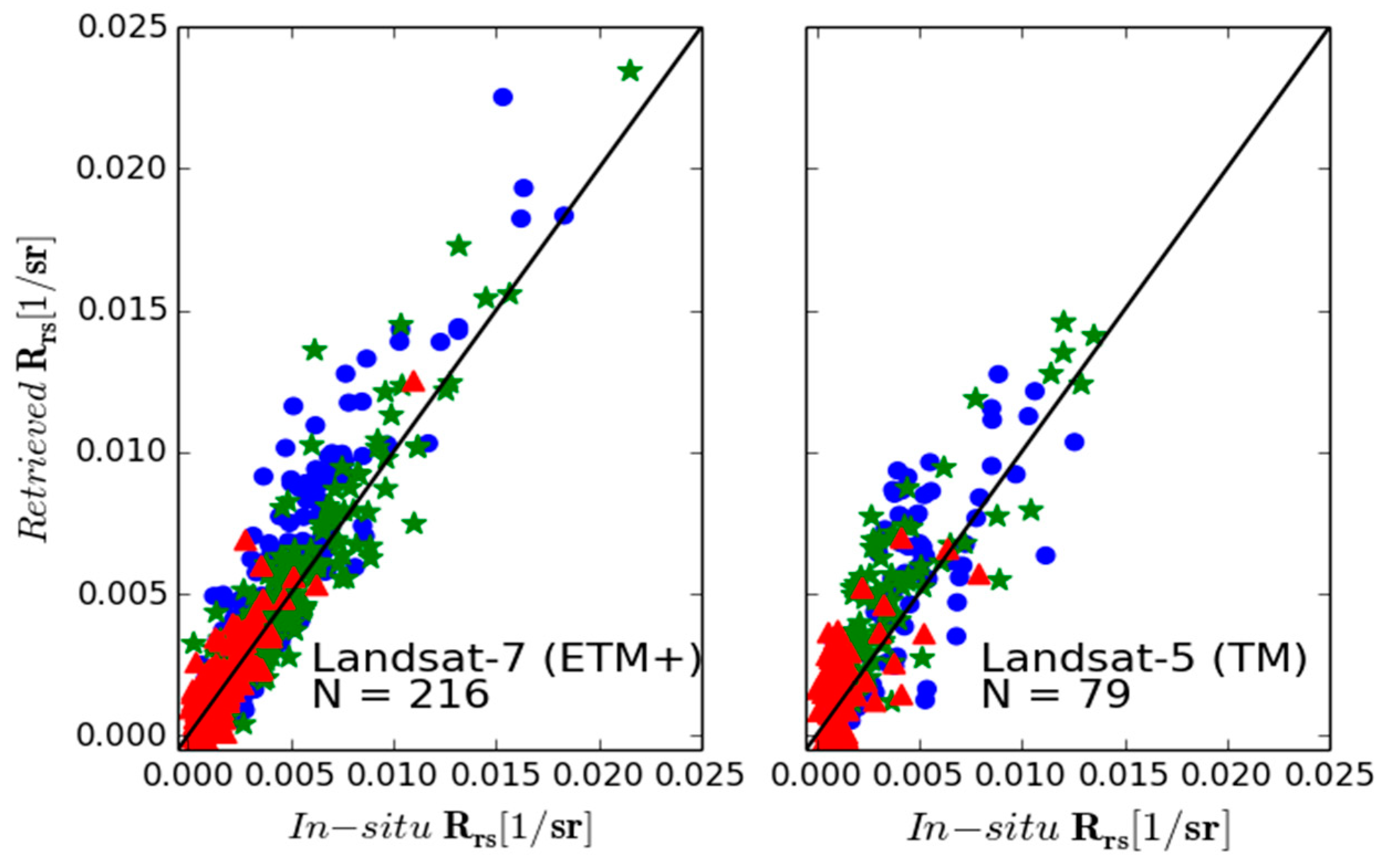
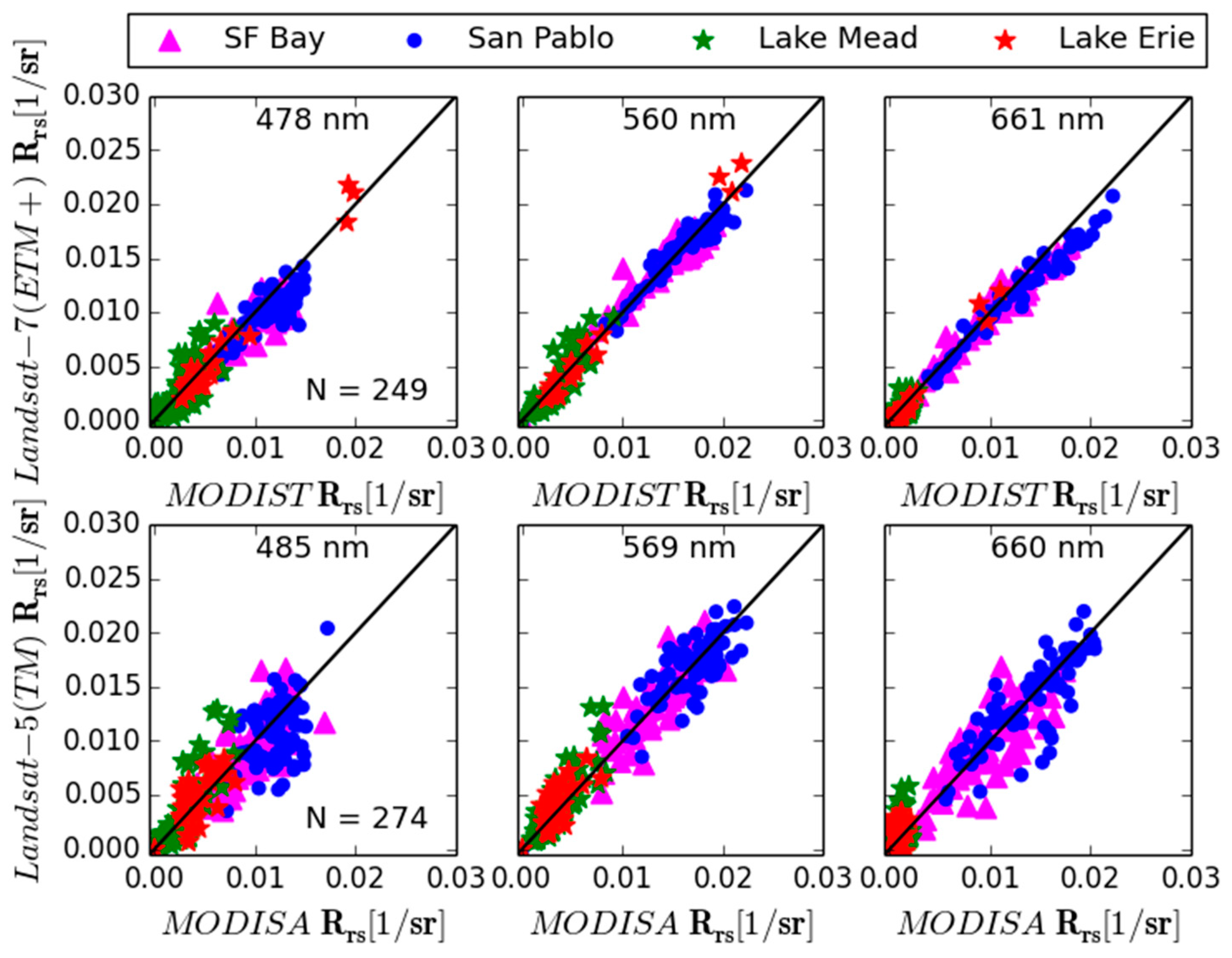
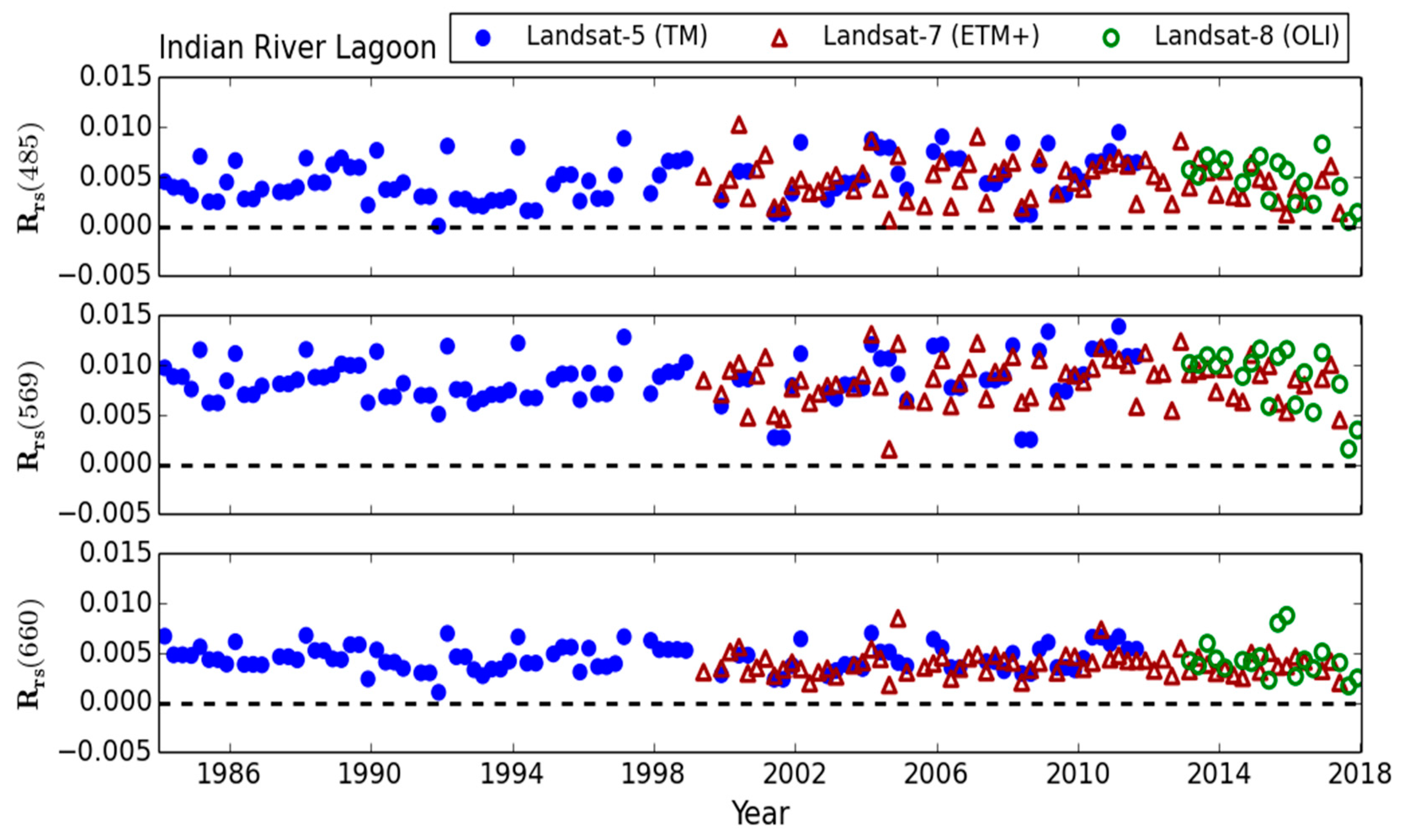
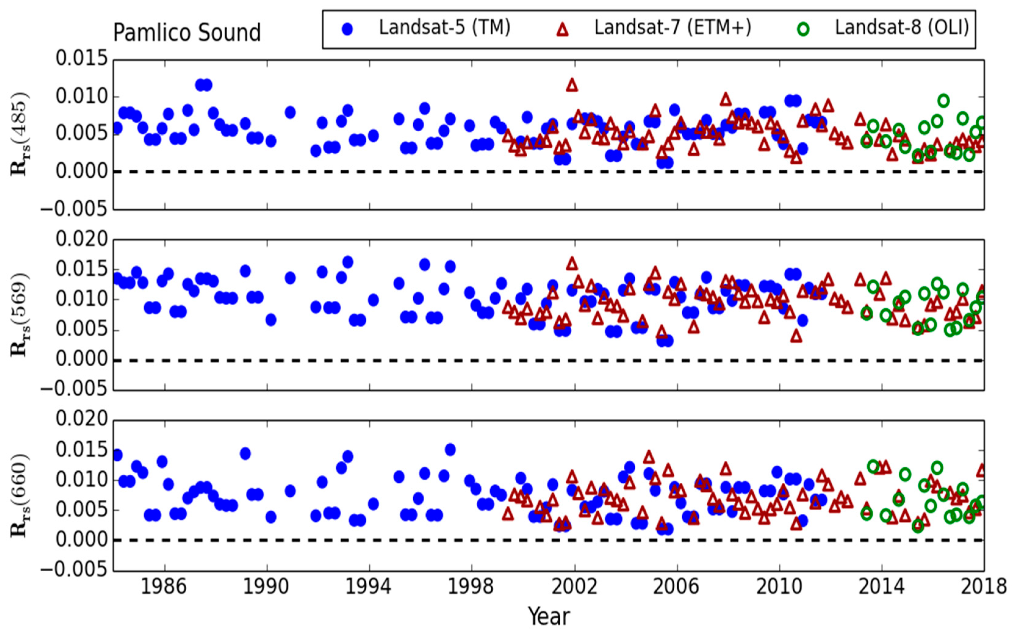
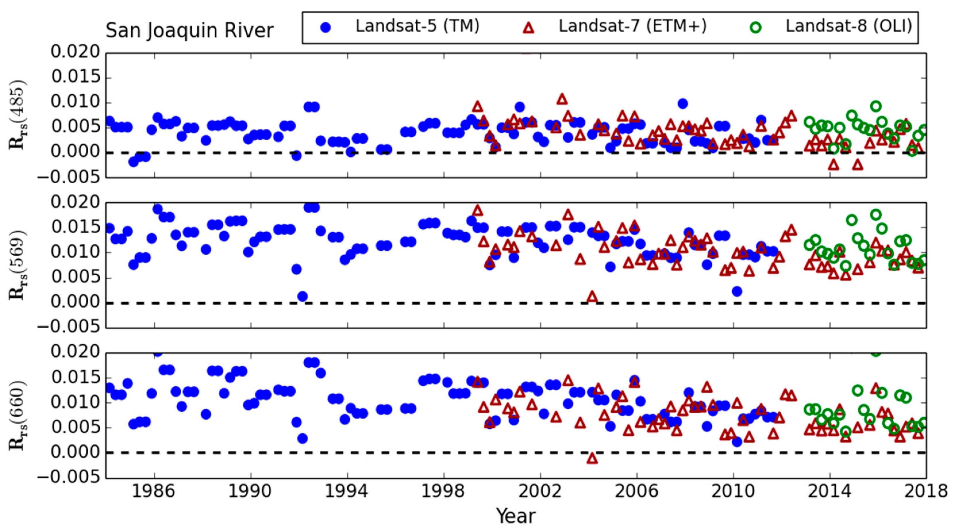
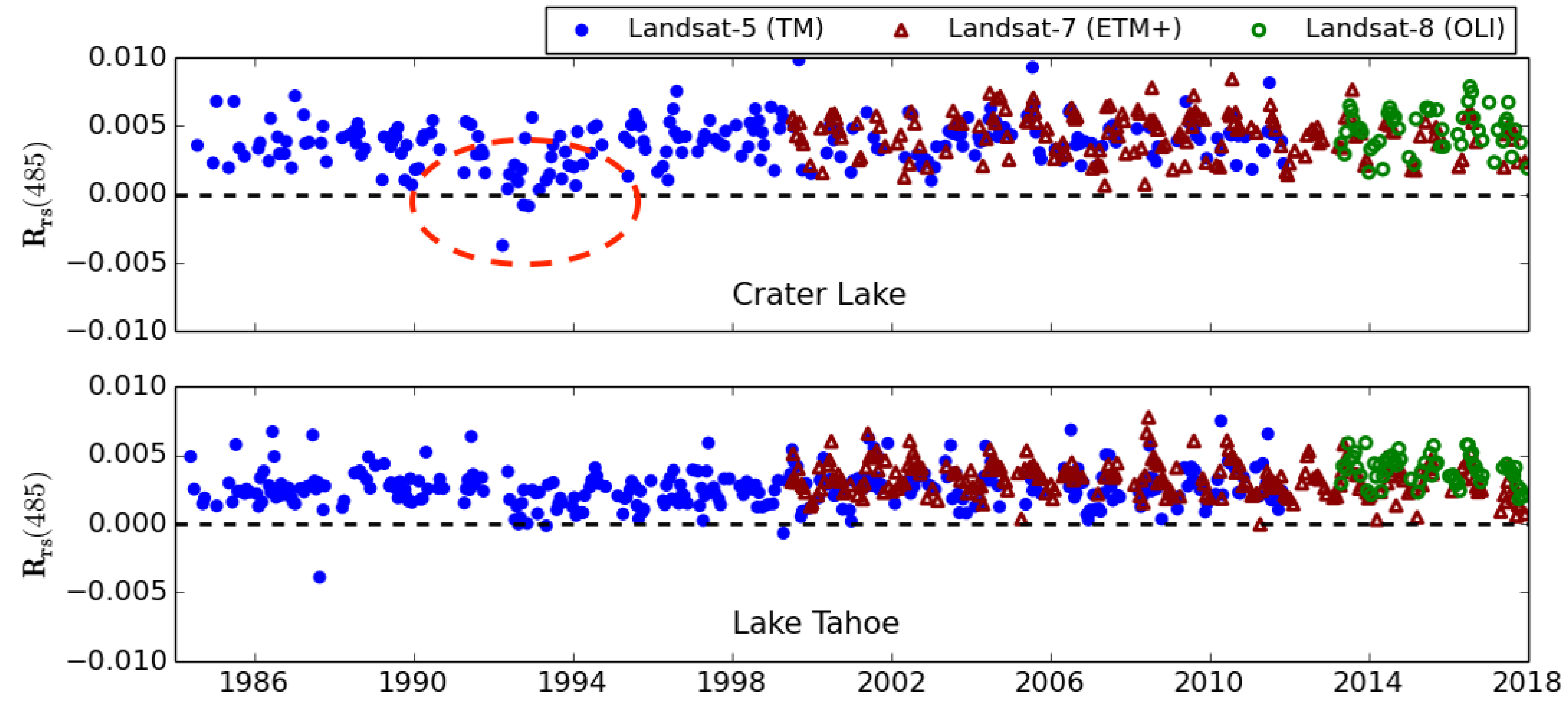
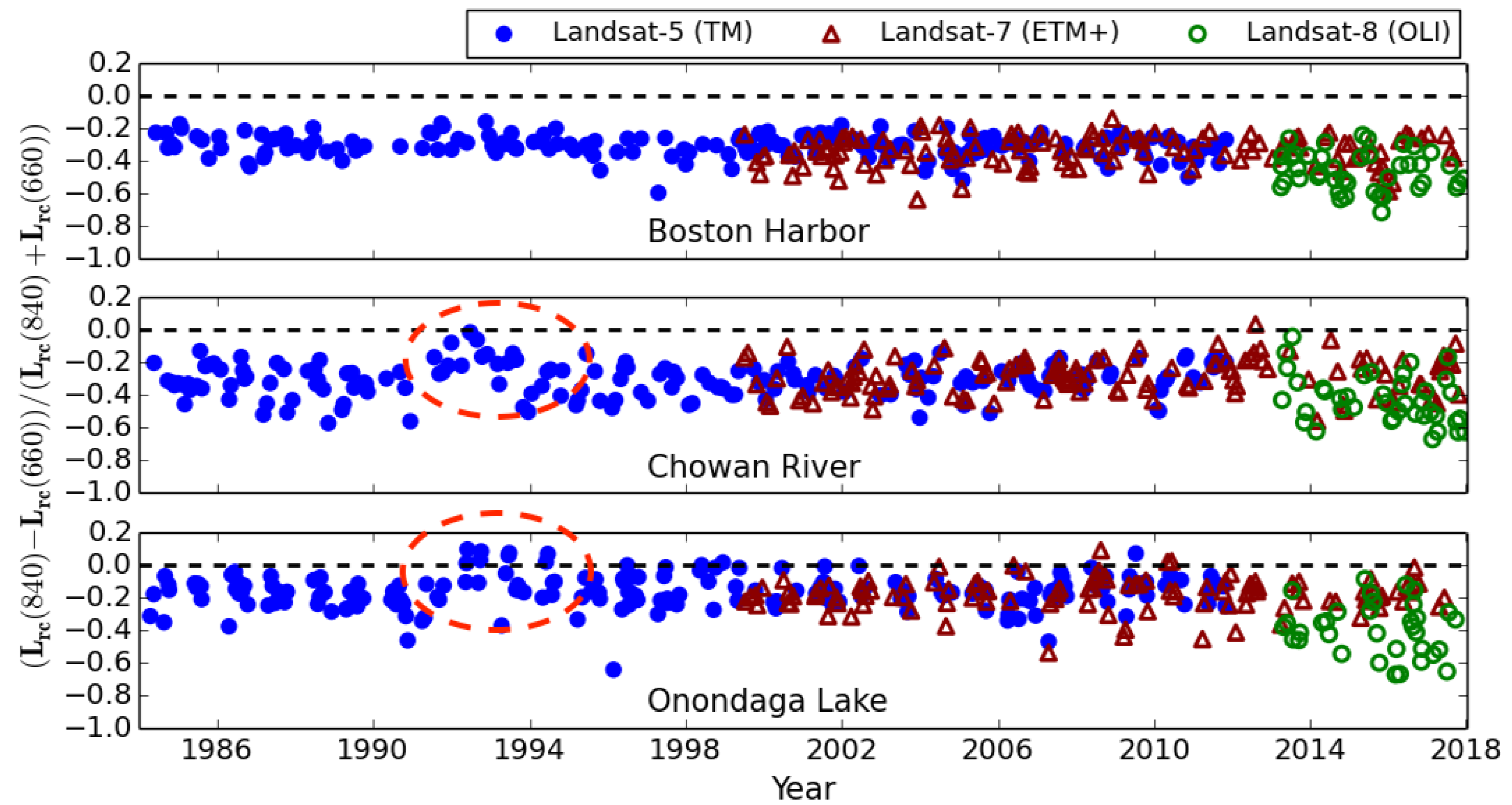
Table 1.
The OLI, ETM+ and TM spectral band centers (nm) computed in SeaDAS.
| Blue [nm] | Green [nm] | Red [nm] | NIR [nm] | SWIR-I [nm] | SWIR-II [nm] | |
|---|---|---|---|---|---|---|
| OLI | 482 | 561 | 655 | 865 | 1609 | 2201 |
| ETM+ | 478 | 560 | 661 | 835 | 1648 | 2205 |
| TM | 485 | 569 | 660 | 840 | 1676 | 2223 |
Table 2.
The vicarious gains for the ETM+ and TM bands. One-standard deviations are presented in round brackets. Note that these gains are derived from the NIR-SWIR-I band combination. The gains for these two bands are derived in step I.
Table 2.
The vicarious gains for the ETM+ and TM bands. One-standard deviations are presented in round brackets. Note that these gains are derived from the NIR-SWIR-I band combination. The gains for these two bands are derived in step I.
| Sensor | Blue | Green | Red | NIR | SWIR-I | SWIR-II |
|---|---|---|---|---|---|---|
| ETM+ | 1.030 (0.023) | 1.01 (0.021) | 1.0278 (0.022) | 1.002 (0.008) | 0.964 (0.12) | 0.991 (0.15) |
| TM | 1.047 (0.02) | 1.011 (0.024) | 1.0581 (0.032) | 0.956 (0.011) | 1.095 (0.13) | 1.0151 (0.072) |
Table 3.
The final vicarious gains for after slight adjustments made to gains enlisted in Table 2. The adjustments were minimal for the green bands. Note that no change was made to the SWIR-II channels.
Table 3.
The final vicarious gains for after slight adjustments made to gains enlisted in Table 2. The adjustments were minimal for the green bands. Note that no change was made to the SWIR-II channels.
| Sensor | Blue | Green | Red | NIR | SWIR-I |
|---|---|---|---|---|---|
| ETM+ | 1.034 | 1.012 | 1.039 | 0.992 | 1.12 |
| TM | 1.059 | 1.011 | 1.058 | 0.931 | 1.21 |
Table 4.
The statistics associated with matchup analyses of Landsat-7 and -5 at AERONET-OC sites. The values in round brackets refer to statistics derived prior to implementing the gains listed in Table 3. The large RMSEs and deviations of slopes from unity are associated with random and systematic errors in TM and ETM+ observations. The Landsat-5 matchups are available only for the last eight years of the mission.
| Band Center [nm] | MRD [%] | RMSE [1/sr] | Slope | Intercept | Bias [1/sr] | R2 |
|---|---|---|---|---|---|---|
| Landsat-7 (ETM+) | ||||||
| 478 | 9.81 (−33.8) | 0.0018 (0.0022) | 1.25 | −0.000016 | 0.0006 | 0.79 |
| 560 | 3.4 (−7.9) | 0.0013 (0.0015) | 1.10 | −0.000024 | 0.000099 | 0.81 |
| 661 | 1.07 (−46.5) | 0.00076 (0.0011) | 1.18 | −0.000014 | 0.0000111 | 0.64 |
| Landsat-5 (TM) | ||||||
| 485 | 13.6 (−85.5) | 0.0020 (0.006) | 1.17 | 0.000013 | 0.00072 | 0.56 |
| 569 | 11.9 (−14.7) | 0.0016 (0.002) | 1.04 | 0.00101 | 0.00082 | 0.85 |
| 660 | 10.1 (−116.2) | 0.00101 (0.003) | 1.14 | 0.0002 | 0.00011 | 0.59 |
Table 5.
The statistics associated with TM-MODIS (n = 274) and MODIS-ETM+ (n = 249) over select sites across North America. Uncertainties associated with the intercomparisons are attributed to atmospheric correction and spectral band adjustments.
Table 5.
The statistics associated with TM-MODIS (n = 274) and MODIS-ETM+ (n = 249) over select sites across North America. Uncertainties associated with the intercomparisons are attributed to atmospheric correction and spectral band adjustments.
| Band Center [nm] | MRD [%] | RMSD [1/sr] | Slope | Intercept | Bias [1/sr] | R2 |
|---|---|---|---|---|---|---|
| Landsat-7 (ETM+) | ||||||
| 478 | −9.56 | 0.00152 | 0.923 | −0.000017 | −0.00044 | 0.91 |
| 560 | −3.29 | 0.00103 | 1.007 | −0.00021 | −0.0002 | 0.97 |
| 661 | −8.15 | 0.00102 | 0.939 | −0.000057 | −0.000039 | 0.98 |
| Landsat-5 (TM) | ||||||
| 485 | −7.11 | 0.002283 | 0.984 | −0.00025 | −0.00033 | 0.76 |
| 569 | −1.83 | 0.001708 | 1.012 | −0.000048 | −0.00017 | 0.93 |
| 660 | 1.97 | 0.001905 | 0.981 | 0.000228 | 0.0000361 | 0.91 |
Table 6.
The SNR, TOA radiance ( ), and the uncertainties in () associated with TM, ETM+, OLI, and MODIS. represents one standard deviation corresponding to the distributions derived from many SeaDAS runs for a small OLI subset. Note that the aerosol removal was conducted using the 840–1676 band combination and OLI’s SNR from [74] were scaled to provide comparable SNRs estimated for typical radiances reported in Reference [5] for TM, ETM+, and MODIS. The units for and are and , respectively. Band centers refer to TM channels.
| Band (nm) | 485 | 569 | 660 | 840 | 1676 | |||
|---|---|---|---|---|---|---|---|---|
| SNR | SNR | SNR | SNR | |||||
| TM | 71.8 | 42.3 | 29.0 | 16.6 | 10.3 | |||
| ETM+ | 77.9 | 69.7 | 40.7 | 13.2 | 10.3 | |||
| OLI | 382.8 | 256.9 | 135.1 | 58.9 | 17.6 | |||
| MODIS | 2209.2 | 2401.8 | 1422.0 | 994.5 | 31.5 | |||
| 54.2 | 29.9 | 15.2 | 4.3 | 0.30 | ||||
| 0.0031 | 0.0028 | 0.0028 | NA | NA | ||||
© 2018 by the authors. Licensee MDPI, Basel, Switzerland. This article is an open access article distributed under the terms and conditions of the Creative Commons Attribution (CC BY) license (http://creativecommons.org/licenses/by/4.0/).
Share and Cite
MDPI and ACS Style
Pahlevan, N.; Balasubramanian, S.V.; Sarkar, S.; Franz, B.A. Toward Long-Term Aquatic Science Products from Heritage Landsat Missions. Remote Sens. 2018, 10, 1337. https://doi.org/10.3390/rs10091337
AMA Style
Pahlevan N, Balasubramanian SV, Sarkar S, Franz BA. Toward Long-Term Aquatic Science Products from Heritage Landsat Missions. Remote Sensing. 2018; 10(9):1337. https://doi.org/10.3390/rs10091337
Chicago/Turabian StylePahlevan, Nima, Sundarabalan V. Balasubramanian, Sudipta Sarkar, and Bryan A. Franz. 2018. "Toward Long-Term Aquatic Science Products from Heritage Landsat Missions" Remote Sensing 10, no. 9: 1337. https://doi.org/10.3390/rs10091337
Note that from the first issue of 2016, this journal uses article numbers instead of page numbers. See further details here.