Numerical Analysis of Microwave Scattering from Layered Sea Ice Based on the Finite Element Method


Department of Physics and Technology, UiT The Arctic University of Norway, 9019 Tromsø, Norway
*
Author to whom correspondence should be addressed.
Remote Sens. 2018, 10(9), 1332; https://doi.org/10.3390/rs10091332
Submission received: 18 July 2018
/
Revised: 13 August 2018
/
Accepted: 17 August 2018
/
Published: 21 August 2018
(This article belongs to the Special Issue Combining Different Data Sources for Environmental and Operational Satellite Monitoring of Sea Ice Conditions)
Abstract
:A two-dimensional scattering model based on the Finite Element Method (FEM) is built for simulating the microwave scattering of sea ice, which is a layered medium. The scattering problem solved by the FEM is formulated following a total- and scattered-field decomposition strategy. The model set-up is first validated with good agreements by comparing the results of the FEM with those of the small perturbation method and the method of moment. Subsequently, the model is applied to two cases of layered sea ice to study the effect of subsurface scattering. The first case is newly formed sea ice which has scattering from both air–ice and ice–water interfaces. It is found that the backscattering has a strong oscillation with the variation of sea ice thickness. The found oscillation effects can increase the difficulty of retrieving the thickness of newly formed sea ice from the backscattering data. The second case is first-year sea ice with C-shaped salinity profiles. The scattering model accounts for the variations in the salinity profile by approximating the profile as consisting of a number of homogeneous layers. It is found that the salinity profile variations have very little influence on the backscattering for both C- and L-bands. The results show that the sea ice can be considered to be homogeneous with a constant salinity value in modelling the backscattering and it is difficult to sense the salinity profile of sea ice from the backscattering data, because the backscattering is insensitive to the salinity profile.
1. Introduction
As a critical component of the earth, sea ice influences the environment, wildlife, human activity, shipping navigation, and natural resource exploration in polar regions and is highly sensitive to global climatic changes. Moreover, there has been a dramatic decline in the Arctic sea ice over the past few decades [1] that has increased the demand for reliable detection and characterization of sea ice.
The technology of high resolution Synthetic Aperture Radar (SAR) has been extensively used to monitor sea ice due to its all-day and all-weather capabilities. To better interpret sea ice from SAR, the link between the physical parameters of sea ice and the SAR signature needs to be built. Electromagnetic (EM) modelling studies can be undertaken to simulate the expected backscattering from hypothetical sea ice scenarios. Through models, the measured SAR signature of sea ice can be related to its geophysical properties. In addition, we can study the differences of SAR signatures under different frequencies, which is instructive to combining multi-frequency SAR data for better monitoring sea ice. A lot of models have been developed to study the scattering from sea ice. Good reviews of models used for simulating microwave scattering from sea ice were provided in refs. [2,3]. The proposed models were utilised to simulate the surface and the volume scattering within the sea ice and the snow cover above, but there is still a lack of study on scattering from the subsurface structures of sea ice. For newly formed sea ice, the incident wave may penetrate through the sea ice and reach the sea water. In this case, the scattering from sea water is inevitable, and the scattering medium should be seen as a layered structure which is composed of sea ice and sea water. Although some models include the scattering from sea water, how the sea water layer influences the total scattering still needs exploring. Another case is first-year sea ice with a typical C-shaped salinity profile [4]. Many models assume that the sea ice is a homogeneous medium with a constant permittivity, but the variation in the salinity profile results in depth-dependent permittivity. To account for the scattering appropriately, it is important to study the effect of variation in the salinity profile. Recently, different scattering models have been used to study the influence of moisture profiles on the backscattering of layered soil [5,6]. To the best of our knowledge, the influence of salinity profiles on the backscattering from sea ice has not been studied.
The objective of this paper is to develop a scattering model that can account for layered structures and demonstrate how the subsurface structure influences the backscattering. Examples of past models that have been used for modelling layered structures include analytic models and numerical models. In terms of analytic models, multilayer small perturbation methods (SPM) have been proposed for calculating the scattering from layered mediums with an arbitrary number of rough interfaces [7,8,9]. With the improvement of computation efficiency, many numerical models have been developed, such as the layered method of moment (MoM) [10] and the finite-volume time-domain method [11]. In this study, we introduce a two-dimensional (2D) numerical model based on the Finite Element Method (FEM). The FEM is applied to the numerical modelling of physical systems in a wide variety of engineering disciplines. This approach has been used to study the scattering from soil [6] and a target above rough sea surfaces [12]. We tailor the FEM for layered sea ice by introducing the concept of total- and scattered-field decomposition (TSFD). The parameters related to the computational time and the accuracy are examined to optimize the FEM based model, which could be instructive in building an efficient and accurate numerical model.
In this paper, a simplified two-dimensional scattering model is built to study the scattering from a one-dimensional (1D) sea ice surface instead of a three-dimensional (3D) model with a 2D surface. The 3D model describes the real word and is able to simulate the meaningful backscattering coefficient, which is comparable to the SAR data. However, the 3D model has a higher-order complexity and needs much more computational time and memory than a 2D model, especially for the scattering simulations of sea ice with a set of varying geophysical parameters. Compared with the scattering from 2D surfaces, the scattering from 1D surfaces shows the same trend as a function of the surface roughness, correlation length, dielectric constant, and incidence angle for surfaces with isotropic roughness [6,13]. Thus, we restrict the model to 2D to provide instructive simulation results efficiently.
The paper is organized as follows. Section 2 details the procedure of the FEM for the simulation of sea ice scattering. The validation of the FEM model is given in Section 3. Section 4 describes the application of the FEM on two different types of sea ice, and Section 5 presents the conclusions of the paper.
2. FEM for Scattering Simulations from Sea Ice
The FEM is a numerical technique for finding approximate solutions to Partial Differential Equations (PDE) by dividing the whole computational domain into subdomains of simple geometry called finite elements. Through the FEM, the PDE problems can be translated into a set of linear algebraic equations [14]. We give an introduction on how to formulate the FEM for sea ice scattering.
2.1. Formulation of the FEM
For scattering problems, the FEM can be formulated in terms of either the total field or the scattered field [15]. The difference between total field and scattered field formulations is how the incident wave is excited. For total field formulation, the incident wave is excited by a source away from the surface of scatterers. Dispersion errors will occur as the incident wave propagates through the domain composed of elements. The scattered field formulation supposes that the background field is known everywhere in the computational domain, and the scattered field is the unknown to be solved. In this case, the incident wave is defined and introduced directly on scatterers.
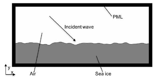
In our problem, the scattering medium is the sea ice, which has a semi-infinite geometry, as depicted in Figure 1. If the scattered field formulation is applied, we need to know the background field in the sea ice, which is difficult to acquire. Consequently, we introduce a strategy using TSFD. The TSFD concept has been widely applied within the finite-difference time-domain [16] and introduced into the time-domain FEM [17] for solving scattering problems. In this study, we apply the TSFD on the frequency-domain FEM and simulate the scattering from the sea ice.
The starting point is the weak form of the electromagnetic wave equation based on the Galerkin method [15,18]. The computational domain is divided into two parts: the area outside the scatter (the air domain) and the area inside the scatter (the sea ice domain). In the air domain , the weak form of the wave equation is expressed based on the scattered field formulation:
where is the electric field of the incident wave, is the electric field of the scattered wave, is called the test function, is the wavenumber in free space, is the boundary of the domain , is the outward normal to the boundary, and and are the relative permeability and relative permittivity of the air domain. Time-harmonic variation of the electromagnetic fields is assumed. In the sea ice domain , the total field formulation is applied and the weak form is expressed as
where is the electric field of the transmitted wave in the sea ice medium, is the boundary of the domain , and and are the relative permeability and relative permittivity of the sea ice domain. The two different formulations are coupled through boundary conditions at the air–ice interface.
By using a Perfect Matched Layer (PML) as the boundary to truncate the computational domain, Equations (1)–(2) can be solved through the FEM. To implement the FEM, the incident wave needs to be defined, which could be a plane wave for simplicity. However, the introduction of a plane wave can cause errors due to reflections from the edges of a finite surface. The commonly used approach to reduce edge effects is the application of tapered waves or the periodic boundary condition (PBC). In this study, we used the Thorsos tapered wave [19] as the incident wave instead of introducing the PBC. This tapered wave can satisfy the wave equation well by appropriate choice of the beam half waist. For the case of horizontal (H) polarization, the incident electric field is defined as
where
represents the out-of plane direction and j is . is defined as the incident angle. g is a parameter that controls the tapering of the wave. A lot of papers [13,20] have discussed how to choose g properly. In this study, we set for all the simulations, where L is the lateral length of the rough sea ice surface. The choice is sufficient to ensure that the tapered wave approximates the solution of the wave equation. For the case of vertical (V) polarization, the incident electric field is defined as
2.2. Rough Surface Generation
For scattering simulations, random rough surfaces must be generated for the FEM computations. A random rough surface is the result of a random process and is usually characterized using the height distribution function (HDF) based on the probability theory. The HDF describes height deviations from the root-mean-square height (denoted as ) in the vertical direction. The surface variation in lateral directions can be described by the autocovariance function (ACF) which is associated with the correlation length (). Commonly used ACFs include the Gaussian and the exponential function. We assumed a Gaussian distribution for the sea ice model, since there is little information about the exact surface statistics. A method using the discrete fast Fourier transform [21] was employed to generate random rough surfaces.
2.3. Numerical Calculation
To numerically solve (1)–(2), the domain was fractured into triangles using the Delaunay algorithm [22]. The second-order Whitney elements were used as basis functions for expanding unknown fields. In the Galerkin method, the basis functions are the same as the test functions. The system of equations was converted into a purely sparse matrix which can be solved directly using the matrix MUltifrontal Massively Parallel sparse direct Solver (MUMPS) [23]. The calculated scattered fields along the inner boundary of the upper PML in the air domain were transformed to far fields by using the Stratton–Chu formulation [24]. Following the derivation in ref. [13], the bistatic radar cross section (RCS) was defined in proper normalization
where is the scattered angle, and is the electric field of the scattered wave at the far field. The RCS is expressed on the decibel (dB) scale by taking the logarithmic transformation. Backscattering RCS can be obtained if . We denote the backscattering RCS at HH and VV polarizations as and , respectively. It should be noted that the scattering for cross polarizations cannot be simulated because the electric field and the magnetic field are completely decoupled for the 2D model.
The calculated bistatic RCS is random because the rough surface is described by stochastic processes [25]. A commonly used method for removing the stochastic fluctuations is the Monto Carlo method. The strategy is to generate a number of different rough surfaces with the same roughness parameters. The scattered fields are then simulated for every surface realization. The final result is obtained by taking the ensemble average of the scattered fields.
3. Model Validation and Selection of Parameters
Before applying the developed FEM model to the study of sea ice scattering, we need to assess the accuracy of the model. Firstly, the FEM model was utilised to simulate the scattering from the homogeneous sea ice with one rough surface. The results were compared with predictions from the first-order SPM [26,27]. Since the model needed to be used to study the scattering of layered sea ice, it was also applied to a layered structure with two rough surfaces for validation. The simulated RCS results were compared with those of a layered MoM [10].
3.1. Comparison of FEM with SPM for Homogeneous Sea Ice
The SPM is only valid for relatively smooth surfaces, where the roughness should satisfy the conditions and [28]. With this restriction of the SPM model, the parameters set for the surface roughness were m and m. Compared with roughness measurements of experimentally grown sea ice [29,30], the chosen parameters were within the reasonable range. The simulated rough surface was in length and was generated by connecting straight line points that were apart. is the wavelength of the incident wave in the air domain. The bistatic RCS were simulated for both C-band ( = 5.6 cm) and L-band ( = 24 cm) waves.
To get the dielectric property of sea ice, empirical dielectric models were used. Most methods calculate the dielectric constant of sea ice from the temperature and salinity data, which can be obtained from in situ measurements. As an important parameter of sea ice, the brine volume fraction influences the permittivity significantly and was calculated from the temperature and salinity based on the equation presented in ref. [31]. The brine volume fraction and temperature were then used to calculate the permittivities of the brine and the ice according to the expressions presented in refs. [32,33,34]. Finally, the permittivity of sea ice was estimated using the Polder–Van Santen–de Loor (PVD) model [35] assuming random oriented needle brine pockets. In this simulation, the temperature and the salinity of sea ice were −2.4 C and 3.5 part per thousand (ppt), which were obtained from measurements of the first-year sea ice at Van Keulenfjord in the Svalbard area [36]. The calculated relative permittivities were and at C- and L-bands.
Monte Carlo simulations were then performed, and ensemble-averaged bistatic RCS results were calculated as a function of the scattering angle for a fixed incidence angle (), from a total of 200 instances of rough surfaces. The HH and VV results at C- and L-bands were compared with the SPM predictions in Figure 2 and Figure 3, and overall, good agreements were observed for both polarizations and frequencies. It should be noted that SPM results lack the realistic peak in the specular direction because the first-order SPM only accounts for incoherent scattering, while the FEM can simulate both coherent and incoherent scattering.
3.2. Comparison of FEM with MoM for Layered Sea Ice
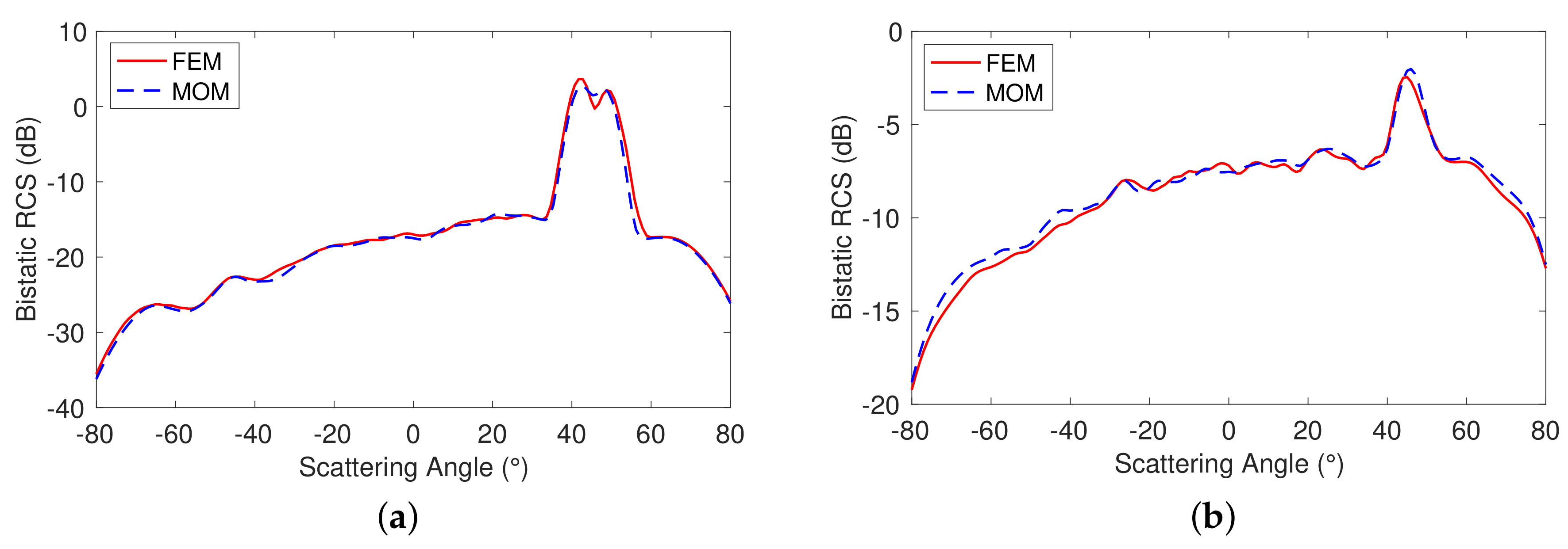
The FEM model can be easily extended to simulate the scattering from layered structures. In this study, the model was used to calculate the scattering from a two-layer structure with two rough surfaces. The results were compared with the predictions from the MoM proposed in ref. [10]. Compared with the FEM, the MoM is less computational intensive, but it is difficult to apply to scattering from many layers due to its surface meshing technique. Both the FEM and the MoM are numerical methods which have no limitation for the surface roughness. Consequently, we simulated the scattering for both slightly rough surfaces and moderately rough surfaces for validation of the FEM model.
Random, but not realistic, sea ice parameters were set for the model because the purpose of the simulations was for validation of the FEM for a range of related variables. The relative permittivity of the first layer was set as 2.25 and the second layer as 4. The distance between the first surface and the second surface was 0.2 m. For the case of slightly rough surfaces, the roughness parameters for the first surface were m and m, and for the second surface, they were m and m. For the case of moderately rough surfaces, the roughness parameters for the first surface were m and m, and for the second surface, they were m and m. Monte Carlo simulations were then performed, and Figure 4 shows the ensemble-averaged bistatic RCS results at C-band as a function of the scattering angle for a fixed incidence angle () and a total of 200 instances of rough surfaces. The results for slightly and moderately rough surfaces from the FEM model were compared with MoM predictions, and overall, good agreements were observed for both cases. It is obvious that the scattering from the moderately rough surfaces was much larger than that from the slightly rough surfaces. Like the first experiment for homogeneous sea ice, the results of L-band and VV polarizations also showed good agreements and are not shown here.
To show that the model can also be adapted to layered sea ice with realistic parameters, it was tested on a sea ice scenario in the Beaufort Sea [11]. The sea ice was newly formed lead ice with a thickness of 9 cm. A slushy layer that was around 1 mm in depth was on the top of the sea ice. The estimated roughness parameters for the slushy layer were m and m. The calculated relative permittivities were for the slushy layer and for the sea ice layer at C-band. The FEM and MoM were used to simulate the scattering from this layered structure for HH polarization. The results are shown in Figure 5 for the ensemble-averaged bistatic RCS as a function of the scattering angle for a fixed incidence angle (), and good agreements were achieved.
3.3. Parameter Selection and Computational Time
The FEM method is computer-intensive and time-consuming because of the use of the Monte Carlo method. The parameters related to the computational time, such as the geometry size and the mesh size of the model, should be chosen carefully. A range of values were selected for these parameters to examine how to make the model efficient, while keeping the accuracy of the result.
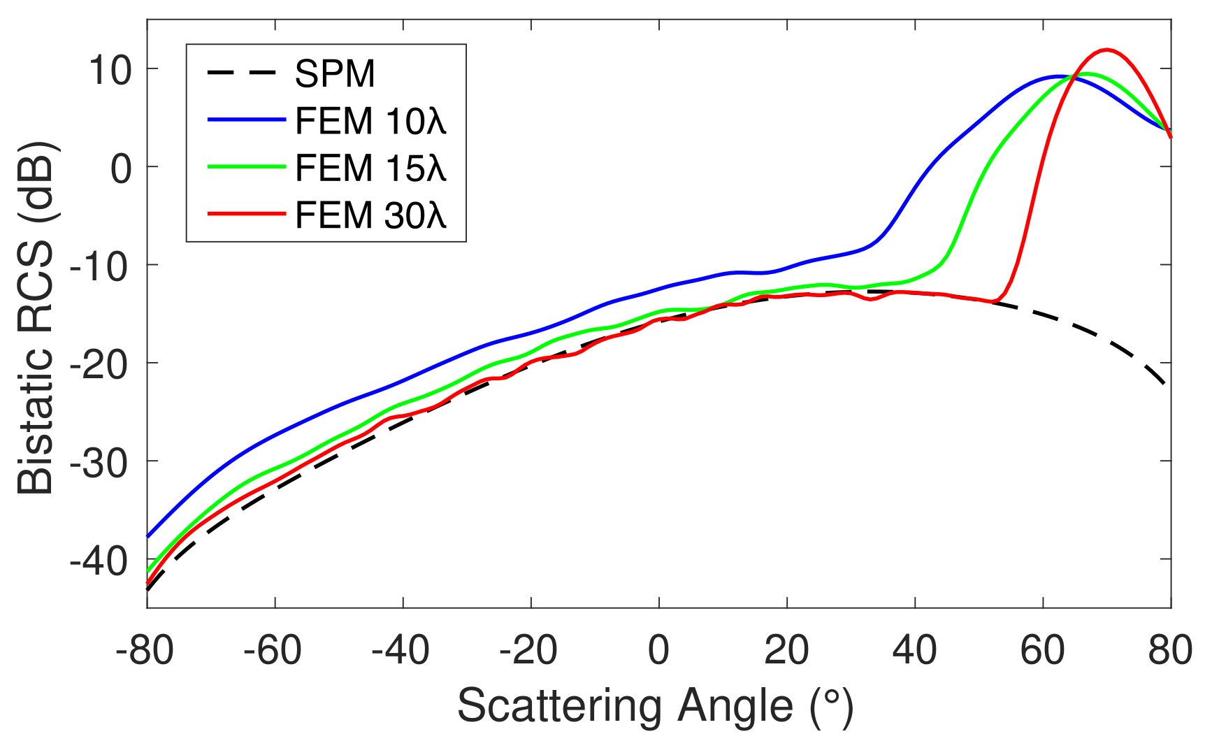
The lateral length of the rough surface determines the size of the computational area and is an important parameter in the numerical model. In general, the surface size should be larger than a few wavelengths to represent the statistic roughness of the surface. However, a larger size is needed at large incidence angles, since a tapered incident wave is used to reduce the edge effects. The tapered incidence wave is no longer an approximation to the solution of the wave equation if the incidence angle is very large. To keep a realistic description of the incident field, the length of the surface must be increased. We simulated the bistatic RCS for an incidence angle of 70° under different surface sizes. The roughness and the permittivity used were the same as the data in the first experiment, and C-band ( = 5.6 cm) was chosen for the wavelength. Figure 6 shows the results from the SPM and the FEM by using three different surface sizes: 10, 15, and 30. It can be seen that surface size with 10 resulted in a large bias compared with the SPM results. When the surface size was 15, the FEM results were higher than the SPM results by 1–4 dB. In the case of surface sizes with 30, the differences between FEM and SPM results were smaller—around 1 dB. Consequently, the incidence angle was up to 70° for simulations in this study, and the chosen surface size needed to be at least 30. Larger surface sizes are needed when the incidence angle is larger than 70°. In particular, when the incidence angle is near grazing angles, a surface size of a few hundred or thousand wavelengths is required for simulations [37].
For the vertical direction, the distance between the upper side of the PML and the rough sea ice surface needs to be decided. The PML should be sufficiently far away so that all evanescent waves disappear and only propagating waves remain. In general, one wavelength of the incidence wave is recommended for the distance. Through experiments, almost the same results can be obtained if the distance is set as small as for some cases. To make sure the result is correct, we chose one wavelength for all the simulations in this study.
Another important factor that influences the efficiency of the FEM model is the mesh size which is the maximum edge length of the triangular element. The mesh size determines the number of finite elements and degrees of freedom. In general, the mesh size should be smaller than for electromagnetic problems. It was determined that was sufficient for generating accurate results in our scattering problem. The results using as maximum mesh size were similar to those using and . It should be noted that only elements in the air domain may use as the maximum size. The required element size should be proportionally smaller in the sea ice medium related to the refractive index. Additionally, elements around the rough surface should be also small enough to capture the small scale roughness of the surface.
When the Monto Carlo method is used, a number of rough surface realizations need to be conducted to get the final result. The number of surface realizations for achieving convergence differs a lot for different simulations, because it depends on all the other parameters that are involved. We chose different combinations of incidence angles and roughness data for simulations to examine the required number of realizations. The chosen incidence angle was up to 70°, and the of the rough surface ranged from 0.002 to 0.01. The number of realizations used for converging results within 1 dB ranged from around 40 to 150. To make sure the result converged for all the simulations, calculations were performed for 200 different rough surfaces for all cases in this study. For each surface realization, the whole computational domain needs to be re-meshed, which may take a lot of time. The scheme of using a single locally modified mesh can greatly improve the computational efficiency [38] and will be explored in the future.
The FEM model presented in this paper was implemented in the commercial software COMSOL Multiphysics. The simulation for one surface instance included geometry generation, meshing, solving equations, and backscattering calculation and took less than 30 seconds on a MacBook Pro with 16 GB of memory. Parallel computing was also applied on the Monte Carlo simulation to simulate different rough surface instances simultaneously, which decreased the total computational time effectively. Simulations using parallel computing require a lot of memory and were performed on a supercomputer [39] which has nodes with 32 GB and 128 GB memory.
4. Model Applications on Sea Ice
4.1. Newly Formed Sea Ice
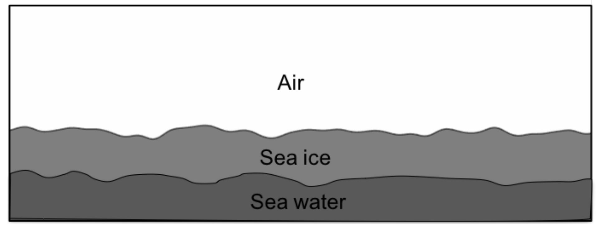
The FEM model was applied on newly formed sea ice to study the influence of the scattering from the sea water interface. Following the definition in [40], newly formed sea ice is the thinnest ice category and includes new ice (frazil, grease, and slush), nilas (0.05–0.10 m thick), and young ice (0.10–0.30 m thick). Figure 7 illustrates the geometry of the scattering problem for the newly formed sea ice experiment. The domain of the sea water can also be replaced by imposing an impedance boundary condition on the ice–water interface, because the sea water has a much larger permittivity than the sea ice [41].
Newly formed ice has various geophysical properties at different growth stages. When the sea ice forms, it contains a high percentage of brine pockets and has a high salinity that results in a high permittivity. With further growth, the salinity drops off quickly. For a wave with 10 GHz, the typical relative permittivities for the new ice and the young ice are and [4], respectively. The penetration depth for the two cases can be calculated based on the following equation [42]:
where is the complex relative permittivity of the sea ice. The penetration depth for the mentioned typical new ice is 0.005 m, which is very small because the imaginary part of the relative permittivity is relatively large. Considering the small penetration depth, only very weak waves may reach the ice–water interface even if the new ice has a very small thickness. Thus, the sea water may not have a large effect on the backscattering from the new ice. To study the influence of sea water, in this paper, we only considered the case of young sea ice.
We used the data in ref. [43] as properties of the young sea ice, of which the temperature was −12.4 C and the salinity was 9 ppt. The temperature and salinity profiles were not available, and the sea ice was assumed to be homogeneous. The surface temperature and salinity for the sea water below the sea ice were −1.83 C and 34.42 ppt, respectively. Using the PVD model, the calculated relative permittivities for the young sea ice were at C-band and at L-band, assuming the brine pockets were randomly oriented needles. The relative permittivities of the sea water were estimated as at C-band and at L-band based on the Klein–Swift model [44]. The roughness parameters for the sea ice surface were set as m and m. There have been few reports about the roughness condition of the ice–water interface, and we considered two different surfaces here. One surface was completely smooth and another one was rough with m and m. The FEM based model was used to simulate the backscattering RCS and co-polarization (co-pol) ratio at an incidence angle of for both C- and L-bands. The co-pol ratio, which describes the scattering differences between the VV and HH channels, was calculated based on the formula [45]
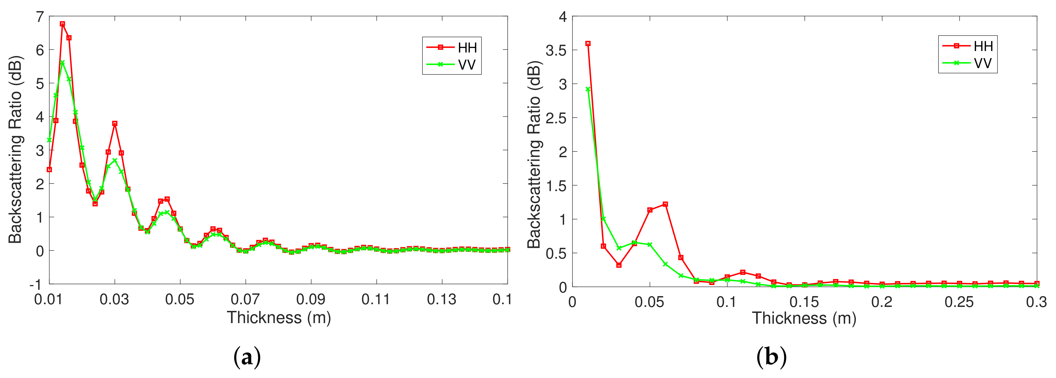
To characterize the effect of the roughness of the sea water surface, we defined a backscattering ratio
where is the total backscattering from sea ice and sea water when the ice–water interface is rough, and is the result for the smooth case. The backscattering ratio describes the influence of the scattering caused by the roughness of the ice–water interface on the total backscattering. The sea water may have different impacts on the backscattering with sea ice thickness variations. To study the effect of the sea water, the thickness of sea ice is another important parameter, and the scattering signatures were simulated within a range of sea ice thicknesses.
The HH and VV backscattering RCS for both smooth and rough ice–water interfaces at C- and L-bands, as a function of the sea ice thickness, are displayed in Figure 8. The results showed strong oscillations as the thickness varied, and the oscillations decayed when the thickness increased. Our scattering model is coherent and able to account for the phase of the waves. The variation in thickness results in phase variations of the wave scattered from the ice–water interfaces. The downgoing and upgoing waves between the air–ice and ice–water interfaces interacted constructively and destructively, depending on the phase differences. The interference had an effect on the total scattered field and caused the oscillatory phenomena. For incidence waves at C-band, we set the range of sea ice thickness from 0 to 0.15 m with a step size of 0.002 m. This step size was small enough to describe all the oscillations at C-band. For the smooth ice–water interface, the HH results oscillated from −15 dB to −25 dB, while the VV results had a range of −20 dB to −15 dB. For the rough case, the HH results oscillated from −22 dB to −13 dB, while the VV results had a range of −17 dB to −12 dB. Overall, the HH results were lower than the VV results, but had a stronger oscillation. The total backscattering for the rough ice–water interface was larger than the results for the smooth interface when the thickness of the sea ice was small. This means that the scattering from the rough ice–water interface has a positive effect on the total backscattering, and the effect will be very small if the sea ice is very thick.
For incidence waves at L-band, the sea ice thickness was set to have a wider range from 0 to 0.3 m with a step size of 0.01 m because of the larger penetration depth. The results for a step size of 0.01 m showed almost the same trend as the results for a step size of 0.002 m at HH polarization. We chose 0.01 m as the step size for all the simulations at L-band and the total simulation time was greatly reduced. For the smooth ice–water interface, the HH results oscillated from −36 dB to −23 dB, while the VV results had a range of −31 dB to −23 dB. For the rough case, the HH results oscillated from −35 dB to −22 dB, while the VV results had a range of −29 dB to −22 dB. Similar to the trends at C-band, the HH results were lower than the VV results, but had stronger oscillation. The stronger oscillations at both C- and L-bands imply that the ice–water interface has a larger effect on the total backscattering at HH polarization than the results at VV polarization. The scattering from the rough ice–water interface increased the total backscattering when the thickness of the sea ice was small. Overall, the backscattering results at C-band were larger than the results at L-band. The oscillation results at C-band had a shorter period and contained more “hills” and “valleys”. This implies that the period of the oscillation is related to the wavelength of the incident wave.
The co-pol ratio results at C- and L-bands are shown in Figure 9. These results also oscillated strongly with the variation in thickness for both C- and L-bands. The oscillation for the rough ice–water interface was weaker than the result for the smooth interface. This indicates that the roughness of the ice–water interface can damp the oscillation and decrease the sensitivity of the total backscattering to the sea ice thickness. A similar oscillatory characteristic of the co-pol ratio was observed by using a 3D scattering model at L-band in ref. [45], which shows that scattering signatures simulated by a 2D model can be comparable to the results simulated by a 3D model.
The backscattering ratio results of the HH and VV polarizations at C- and L-bands are shown in Figure 10. The results describe the backscattering differences with respect to rough and smooth ice–water interfaces. It can be observed that the scattering caused by the rough ice–water interface increased the total backscattering by maximum of 6.8 dB at C-band and 3.6 dB at L-band for HH polarization, compared with scattering from the smooth ice–water interface. The contributions were less for VV polarizations with a maximum of 5.4 dB at C-band and 2.9 dB at L-band. Overall, the contributions due to the roughness of the ice–water interface became smaller when the thickness of the sea ice increased. However, when the thickness was small, the influence of the roughness from the ice–water interface oscillated with the variation in thickness.
The oscillation could show different features if the temperature and salinity are quite different from the parameters used in this study. However, similar results would be expected if the parameters are close, and those results could improve the interpretation of SAR images. It should be noted that the oscillations of the backscattering signatures may be damped on real SAR images because sea ice with different thickness contribute to the total backscattering within each pixel. When oscillating behaviour exists, ambiguous results will be obtained if we want to retrieve the sea ice thickness from the backscattering. The combination of multiple-incidence and multi-frequency data may be used to resolve the ambiguity caused by the subsurface.
4.2. First-Year Sea Ice
First-year sea ice refers to sea ice thicker than 0.3 m and of not more than one winter’s growth [46]. For first-year sea ice, both the temperature and salinity are thickness-dependent. Actually, it is well-known that first-year sea ice may have a C-shaped salinity profile. The dielectric property of sea ice can be determined by its temperature and salinity. It is critical to consider whether the variation in salinity with depth has an impact on the backscattering. To account for this effect, the subsurface profile of the sea ice should be divided into many layers, where the salinity is constant within each layer. Then, the FEM model can be applied to simulate the scattering from the multi-layer sea ice.
In this study, the temperature was assumed to be −15 C at all depths since only the influence from the C-shaped salinity profile was studied. On the surface of first-year sea ice, the salinity can range from 5 ppt to 18 ppt depending on different climatic conditions [47,48]. High surface salinity results in a shorter penetration depth and fewer impacts from the subsurface. Hence, to study the subsurface influence, the salinity of the surface was assumed to be 6 ppt. The salinity at the bottom was assumed to be the same as the surface salinity. In the middle of the sea ice, the salinity was set within a range from 1 ppt to 6 ppt. The thickness of the ice was set as 0.3 m to construct sharp salinity profiles that varied rapidly with respect to the depth. With the chosen parameters, the variation in the realistic salinity profiles could be in the range of the variation of the simulated profiles. As shown in Figure 11, six different salinity profiles were generated by using polynomial curve fitting. To accurately account for the scattering from sea ice with the variation in salinity, the profile was divided into 300 layers, and the salinity and dielectric properties were constant within each layer with a thickness of 0.1 cm. The permittivity was calculated by using the the PVD dielectric model and assuming the brine pockets were randomly oriented needles. It was found that the PVD-based models can be used successfully for first-year sea ice when the random needle brine pockets assumption is used [35]. It should be mentioned that the generated salinity profiles are not based on a sea ice growth scheme and do not correspond to realistic salinity profiles. Instead, the results from the salinity profiles with simple forms will be instructive to more complicated cases. The roughness parameters for the sea ice surface were set as m and m, which are within the realistic range. The FEM model was used to simulate the backscattering from the sea ice with layered salinity profiles at an incidence angle of 30.
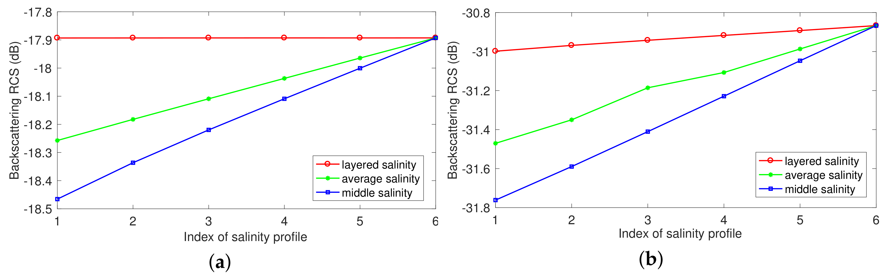
The HH backscattering results for all the different profiles at C-band are shown in Figure 12a. It can be observed that the backscattering from the six different salinity profiles were almost the same. This is because the surface salinity at 6 ppt corresponds to the relative permittivity at and the penetration depth at 0.05 m. The small penetration depth implies that the C-band wave only interacts with the uppermost part of the salinity profile. This suggests that we may only retrieve the surface salinity of sea ice from C-band SAR data. For most cases in sea ice modelling, the sea ice is assumed to be homogeneous with a constant salinity. It is important to examine if it is correct to consider sea ice to be a homogeneous medium. We used the average salinity of the profile and the salinity at the middle depth as the salinity of the homogenous sea ice, and calculated the backscattering for the two cases. From Figure 12a, it can be observed that the results were slightly lower than those of the sea ice with salinity profiles. However, the differences were very small and within 1 dB. The implication of the result is that the backscattering is insensitive to the variation in salinity at C-band.
The results for HH polarization at L-band are shown in Figure 12b. The differences in the backscattering from the six profiles were very small, even though the L-band wave has a much larger penetration depth and can interact with the salinity profiles. The reason for this is that the backscattering from the first-year sea ice is not sensitive to the salinity. It can be observed that the backscattering from homogeneous sea ice with a constant salinity of 1 ppt was slightly lower than the result with a salinity of 6 ppt. We also increased the surface salinity from 6 ppt to 12 ppt and the salinity at the bottom was assumed to be 12 ppt. In the middle of the sea ice, the salinity was set within a range from 1 ppt to 12 ppt. A total of 12 different salinity profiles with sharper salinity variations were generated, and the backscattering from these profiles were almost the same. The salinity at 12 ppt corresponded to the relative permittivity at and the penetration depth at 0.05 m for the L-band wave. With an increase in the salinity, the penetration depth became smaller. The penetration depth was not large enough to make the L-band wave sense the variation in salinity if the surface salinity was equal to or larger than 12 ppt.
A rougher surface with m and m was tested for both C- and L-bands. The differences in the backscattering from the salinity profiles slightly increased but were still within 1 dB. Simulations were conducted for different temperatures: −5 C and −25 C. For each temperature, the backscattering from different salinity profiles were also similar. Compared with the HH polarization results for the six different salinity profiles at −15 C, the backscattering at −5 C increased by around 1.4 dB and 1.6 dB for C-band and L-band, while the backscattering at −25 C decreased by around 0.5 dB and 0.5 dB for C-band and L-band. All the results imply that the variations within the vertical salinity profile have very little impact on the backscattering from the first-year sea ice. When modelling the backscattering of the sea ice with salinity profiles, we can consider the sea ice to be a homogeneous medium with a constant salinity value. Thus, it is difficult to retrieve the salinity profile of the sea ice from the backscattering data.
5. Conclusions
In this paper, a model based on the FEM was built to study the scattering from sea ice. By comparing the proposed model with the SPM and the MoM, it was confirmed that the model can accurately account for the scattering from layered sea ice under multi-incidence and multi-frequency waves. The model was also optimized by examining how to choose best parameters with respect to the computational time whilst maintaining accuracy.
The FEM model was then used to analyse the scattering from the subsurface of sea ice at both C- and L-bands. For newly formed sea ice, the ice–water interface together with the variations in the sea ice thickness resulted in strong oscillations of backscattering signatures. It was found that the oscillatory effects were stronger for HH polarization than VV polarization. The differences in scattering from rough and smooth ice–water interfaces were also examined. The total backscattering increased due to the roughness of the ice–water interface and the backscattering differences between the two scenarios also oscillated with the thickness of the sea ice. The model was then applied to first-year sea ice to study the impact of the C-shaped salinity profile variation on the backscattering. The influence was very small for both C- and L-band waves because of the small penetration depth and the insensitivity of the backscattering to the salinity. All these findings could improve the understanding of microwave interactions with sea ice and interpretations of SAR images over polar areas. The simulations in this study were based on sea ice with a few selected parameters that covered a representative range of real sea ice data. The influence of temperature profiles and different brine shapes on the backscattering should be further analysed. The simulation results for cross polarizations were not available in the model and the volume scattering from brine pockets was neglected. These scattering effects will be further studied in the future.
Author Contributions
X.X. conducted the model development, simulations, results analyses and drafted the manuscript. F.M. provided the technique guidance on electromagnetics and COMSOL. C.B. and A.P.D. were involved in the model applications on sea ice. All authors participated in discussing and editing the manuscript.
Funding
This research received no external funding.
Acknowledgments
This research is partly funded by CIRFA partners and the Research Council of Norway (grant number 237906).
Conflicts of Interest
The authors declare no conflict of interest.
References
- Comiso, J.C. Large Decadal Decline of the Arctic Multiyear Ice Cover. J. Clim. 2012, 25, 1176–1193. [Google Scholar] [CrossRef] [Green Version]
- Golden, K.M.; Cheney, M.; Ding, K.H.; Fung, A.K.; Grenfell, T.C.; Isaacson, D.; Kong, J.A.; Nghiem, S.V.; Sylvester, J.; Winebrenner, P. Forward electromagnetic scattering models for sea ice. IEEE Trans. Geosci. Remote Sens. 1998, 36, 1655–1674. [Google Scholar] [CrossRef]
- Jezek, K.C.; Perovich, D.K.; Golden, K.M.; Luther, C.; Barber, D.G.; Gogineni, P.; Grenfell, T.C.; Jordan, A.K.; Mobley, C.D.; Nghiem, S.V.; et al. A broad spectral, interdisciplinary investigation of the electromagnetic properties of sea ice. IEEE Trans. Geosci. Remote Sens. 1998, 36, 1633–1641. [Google Scholar] [CrossRef] [Green Version]
- Shokr, M.; Sinha, N. Sea Ice: Physics and Remote Sensing; John Wiley & Sons: Hoboken, NJ, USA, 2015. [Google Scholar]
- Konings, A.G.; Entekhabi, D.; Moghaddam, M.; Saatchi, S.S. The effect of variable soil moisture profiles on P-band backscatter. IEEE Trans. Geosci. Remote Sens. 2014, 52, 6315–6325. [Google Scholar] [CrossRef]
- Khankhoje, U.K.; van Zyl, J.J.; Cwik, T.A. Computation of radar scattering from heterogeneous rough soil using the finite-element method. IEEE Trans. Geosci. Remote Sens. 2013, 51, 3461–3469. [Google Scholar] [CrossRef]
- Imperatore, P.; Iodice, A.; Riccio, D. Electromagnetic wave scattering from layered structures with an arbitrary number of rough interfaces. IEEE Trans. Geosci. Remote Sens. 2009, 47, 1056–1072. [Google Scholar] [CrossRef]
- Komarov, A.S.; Shafai, L.; Barber, D.G. Electromagnetic wave scattering from rough boundaries interfacing inhomogeneous media and application to snow-covered sea ice. Prog. Electromagn. Res. 2014, 144, 201–219. [Google Scholar] [CrossRef]
- Tabatabaeenejad, A.; Moghaddam, M. Bistatic scattering from three-dimensional layered rough surfaces. IEEE Trans. Geosci. Remote Sens. 2006, 44, 2102–2114. [Google Scholar] [CrossRef]
- Moss, C.D.; Grzegorczyk, T.M.; Han, H.C.; Kong, J.A. Forward-backward method with spectral acceleration for scattering from layered rough surfaces. IEEE Trans. Antennas Propag. 2006, 54, 1006–1016. [Google Scholar] [CrossRef]
- Isleifson, D.; Jeffrey, I.; Shafai, L.; LoVetri, J.; Barber, D.G. A Monte Carlo method for simulating scattering from sea ice using FVTD. IEEE Trans. Geosci. Remote Sens. 2012, 50, 2658–2668. [Google Scholar] [CrossRef]
- Liu, P.; Jin, Y.Q. Numerical simulation of bistatic scattering from a target at low altitude above rough sea surface under an EM-wave incidence at low grazing angle by using the finite element method. IEEE Trans. Antennas Propag. 2004, 52, 1205–1210. [Google Scholar] [CrossRef]
- Tsang, L.; Kong, J.A.; Ding, K.H.; Ao, C.O. Scattering of Electromagnetic Waves: Numerical Simulations; John Wiley & Sons, Inc.: New York, NY, USA, 2001. [Google Scholar] [CrossRef]
- Dhatt, G.; LefranÃ, E.; Touzot, G. Finite Element Method; John Wiley & Sons: Hoboken, NJ, USA, 2012. [Google Scholar]
- Volakis, J.L.; Chatterjee, A.; Kempel, L.C. Finite Element Method Electromagnetics: Antennas, Microwave Circuits, and Scattering Applications; John Wiley & Sons: New York, NY, USA, 1998; Volume 6. [Google Scholar]
- Taflove, A.; Hagness, S.C. Computational Electrodynamics: The Finite-Difference Time-Domain Method; Artech House: Norwood, MA, USA, 2005. [Google Scholar]
- Riley, D.J.; Jin, J.M.; Lou, Z.; Petersson, L.R. Total-and scattered-field decomposition technique for the finite-element time-domain method. IEEE Trans. Antennas Propag. 2006, 54, 35–41. [Google Scholar] [CrossRef]
- Jin, J. The Finite Element Method in Electromagnetics, 3rd ed.; Wiley-IEEE Press: Hoboken, NJ, USA, 2014. [Google Scholar]
- Thorsos, E.I. The validity of the Kirchhoff approximation for rough surface scattering using a Gaussian roughness spectrum. J. Acoust. Soc. Am. 1988, 83, 78–92. [Google Scholar] [CrossRef]
- Ye, H.; Jin, Y.Q. Parameterization of the tapered incident wave for numerical simulation of electromagnetic scattering from rough surface. IEEE Trans. Antennas Propag. 2005, 53, 1234–1237. [Google Scholar]
- Garcia, N.; Stoll, E. Monte Carlo calculation for electromagnetic-wave scattering from random rough surfaces. Phys. Rev. Lett. 1984, 52, 1798. [Google Scholar] [CrossRef]
- Delaunay, B. Sur la sphere vide. Izv. Akad. Nauk SSSR, Otdelenie Matematicheskii i Estestvennyka Nauk 1934, 7, 1–2. [Google Scholar]
- Mary, T. Block Low-Rank Multifrontal Solvers: Complexity, Performance, and Scalability. Ph.D. Thesis, Toulouse University, Toulouse, France, 2017. [Google Scholar]
- Fung, A.; Li, Z.; Chen, K. Backscattering from a randomly rough dielectric surface. IEEE Trans. Geosci. Remote Sens. 1992, 30, 356–369. [Google Scholar] [CrossRef]
- Tsang, L.; Liao, T.H.; Tan, S.; Huang, H.; Qiao, T.; Ding, K.H. Rough Surface and Volume Scattering of Soil Surfaces, Ocean Surfaces, Snow, and Vegetation Based on Numerical Maxwell Model of 3-D Simulations. IEEE J. Sel. Top. Appl. Earth Observ. Remote Sens. 2017, 10, 4703–4720. [Google Scholar] [CrossRef]
- Chan, C.H.; Tsang, L.; Li, Q. Monte Carlo simulations of large-scale one-dimensional random rough-surface scattering at near-grazing incidence: Penetrable case. IEEE Trans. Antennas Propag. 1998, 46, 142–149. [Google Scholar] [CrossRef]
- Zahn, D.; Sarabandi, K.; Sabet, K.; Harvey, J. Numerical simulation of scattering from rough surfaces: A wavelet-based approach. IEEE Trans. Antennas Propag. 2000, 48, 246–253. [Google Scholar] [CrossRef]
- Ticconi, F.; Pulvirenti, L.; Pierdicca, N. Models for scattering from rough surfaces. In Electromagnetic Waves; InTech: Rijeka, Croatia, 2011. [Google Scholar]
- Beaven, S.; Gogineni, S.; Gow, A.; Lohanick, A.; Jezek, K. Radar Backscatter Measurements from Simulated Sea Ice During CRRELEX’90; Technical Report; University of Kansas: Lawrence, KS, USA, 1993. [Google Scholar]
- Nassar, E.M. Numerical and Experimental Studies of Electromagnetic Scattering from Sea Ice. Ph.D. Thesis, The Ohio State University, Columbus, OH, USA, 1997. [Google Scholar]
- Frankenstein, G.; Garner, R. Equations for determining the brine volume of sea ice from -0.5 to -22.9 °C. J. Glaciol. 1967, 6, 943–944. [Google Scholar] [CrossRef]
- Stogryn, A.; Desargant, G. The dielectric properties of brine in sea ice at microwave frequencies. IEEE Trans. Antennas Propag. 1985, 33, 523–532. [Google Scholar] [CrossRef]
- Matzler, C.; Wegmuller, U. Dielectric properties of freshwater ice at microwave frequencies. J. Phys. D Appl. Phys. 1987, 20, 1623. [Google Scholar] [CrossRef]
- Nyfors, E. On Dielectric Properties of Dry Snow in the 800 MHz to 13 GHz Region; Report S; Helsinki University of Technology: Espoo, Finland, 1982. [Google Scholar]
- Shokr, M.E. Field observations and model calculations of dielectric properties of Arctic sea ice in the microwave C-band. IEEE Trans. Geosci. Remote Sens. 1998, 36, 463–478. [Google Scholar] [CrossRef]
- Kampffmeyer, M.C. Numerical Modeling of Microwave Interactions with Sea Ice. Master’s Thesis, UiT The Arctic University of Norway, Tromsø, Norway, 2014. [Google Scholar]
- Tsang, L.; Chan, C.H.; Pak, K.; Sangani, H. Monte-Carlo simulations of large-scale problems of random rough surface scattering and applications to grazing incidence with the BMIA/canonical grid method. IEEE Trans. Antennas Propag. 1995, 43, 851–859. [Google Scholar] [CrossRef]
- Khankhoje, U.K.; Padhy, S. Stochastic Solutions to Rough Surface Scattering Using the Finite Element Method. IEEE Trans. Antennas Propag. 2017, 65, 4170–4180. [Google Scholar] [CrossRef]
- Stallo. Available online: https://www.sigma2.no/content/stallo (accessed on 1 May 2018).
- Johansson, A.M.; Brekke, C.; Spreen, G.; King, J.A. X-, C-, and L-band SAR signatures of newly formed sea ice in Arctic leads during winter and spring. Remote Sens. Environ. 2018, 204, 162–180. [Google Scholar] [CrossRef]
- Wu, J. Radar Sub-Surface Sensing for Mapping the Extent of Hydraulic Fractures and for Monitoring Lake Ice and Design of Some Novel Antennas. Ph.D. Thesis, University of Michigan, Ann Arbor, MI, USA, 2016. [Google Scholar]
- Ulaby, F.T.; Stiles, W.H.; Abdelrazik, M. Snowcover Influence on Backscattering from Terrain. IEEE Trans. Geosci. Remote Sens. 1984, GE-22, 126–133. [Google Scholar] [CrossRef]
- Melnikov, I. An in situ experimental study of young sea ice formation on an Antarctic lead. J. Geophys. Res. 1995, 100, 4673. [Google Scholar] [CrossRef]
- Klein, L.; Swift, C. An improved model for the dielectric constant of sea water at microwave frequencies. IEEE J. Ocean. Eng. 1977, 2, 104–111. [Google Scholar] [CrossRef]
- Winebrenner, D.; Farmer, L.; Joughin, I. On the response of polarimetric synthetic aperture radar signatures at 24-cm wavelength to sea ice thickness in Arctic leads. Radio Sci. 1995, 30, 373–402. [Google Scholar] [CrossRef]
- Casey, J.A.; Howell, S.E.; Tivy, A.; Haas, C. Separability of sea ice types from wide swath C- and L-band synthetic aperture radar imagery acquired during the melt season. Remote Sens. Environ. 2016, 174, 314–328. [Google Scholar] [CrossRef]
- Eicken, H. Salinity profiles of Antarctic sea ice: Field data and model results. J. Geophys. Res. Oceans 1992, 97, 15545–15557. [Google Scholar] [CrossRef]
- Nakawo, M.; Sinha, N.K. Growth rate and salinity profile of first-year sea ice in the high Arctic. J. Glaciol. 1981, 27, 315–330. [Google Scholar] [CrossRef]
Figure 1.
Geometry illustrating the computational domain for the sea ice scattering.

Figure 2.
Bistatic radar cross section (RCS) of (a) HH and (b) VV polarizations simulated by the Finite Element Method (FEM) and the small perturbation method (SPM) for incidence angle at C-band.
Figure 2.
Bistatic radar cross section (RCS) of (a) HH and (b) VV polarizations simulated by the Finite Element Method (FEM) and the small perturbation method (SPM) for incidence angle at C-band.

Figure 3.
Bistatic RCS of (a) HH and (b) VV polarizations simulated by FEM and SPM for incidence angle at L-band.
Figure 3.
Bistatic RCS of (a) HH and (b) VV polarizations simulated by FEM and SPM for incidence angle at L-band.

Figure 4.
Bistatic RCS for a two-layer structure with (a) slightly rough surfaces and (b) moderately rough surfaces simulated by the FEM and method of moment (MoM) at C-band. The incidence angle was and the polarization was HH.
Figure 4.
Bistatic RCS for a two-layer structure with (a) slightly rough surfaces and (b) moderately rough surfaces simulated by the FEM and method of moment (MoM) at C-band. The incidence angle was and the polarization was HH.

Figure 5.
Bistatic RCS for the slush-covered sea ice simulated by the FEM and MoM at C-band. The incidence angle was and the polarization was HH.
Figure 5.
Bistatic RCS for the slush-covered sea ice simulated by the FEM and MoM at C-band. The incidence angle was and the polarization was HH.

Figure 6.
Bistatic RCS for the HH polarization simulated by the SPM and the FEM under different surface sizes.
Figure 6.
Bistatic RCS for the HH polarization simulated by the SPM and the FEM under different surface sizes.

Figure 7.
Geometry illustrating the newly formed sea ice considered for the scattering simulation.

Figure 8.
Backscattering RCS with respect to the thickness of the newly formed sea ice at an incidence angle of for (a) C-band and (b) L-band. The HH and VV results were simulated for both smooth and rough ice–water interfaces.
Figure 8.
Backscattering RCS with respect to the thickness of the newly formed sea ice at an incidence angle of for (a) C-band and (b) L-band. The HH and VV results were simulated for both smooth and rough ice–water interfaces.

Figure 9.
Co-polarization ratio with respect to the thickness of the newly formed sea ice at an incidence angle of for (a) C-band and (b) L-band.
Figure 9.
Co-polarization ratio with respect to the thickness of the newly formed sea ice at an incidence angle of for (a) C-band and (b) L-band.

Figure 10.
Backscattering ratio of HH and VV polarizations with respect to the thickness of the newly formed sea ice at an incidence angle of for (a) C-band and (b) L-band. The backscattering ratio was defined to describe the scattering difference between smooth and rough ice–water interfaces.
Figure 10.
Backscattering ratio of HH and VV polarizations with respect to the thickness of the newly formed sea ice at an incidence angle of for (a) C-band and (b) L-band. The backscattering ratio was defined to describe the scattering difference between smooth and rough ice–water interfaces.

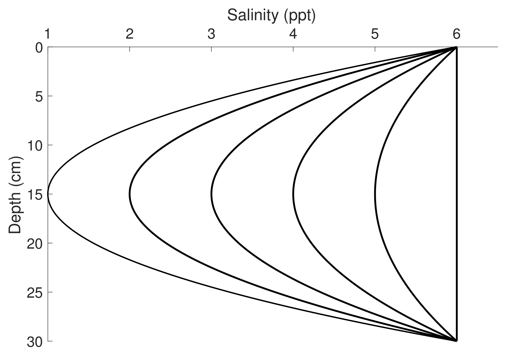
Figure 11.
Graphical representation of six salinity profiles. The top and bottom salinity of first-year sea ice are 6 ppt. The salinity at the middle depth ranges from 1 ppt to 6 ppt.
Figure 11.
Graphical representation of six salinity profiles. The top and bottom salinity of first-year sea ice are 6 ppt. The salinity at the middle depth ranges from 1 ppt to 6 ppt.

Figure 12.
Backscattering RCS of HH polarization for six different salinity profiles at (a) C-band and (b) L-band. The results using the assumption that sea ice is a homogeneous medium with a constant salinity are also plotted by using the average salinity of the profile and the salinity in the middle of the sea ice.

© 2018 by the authors. Licensee MDPI, Basel, Switzerland. This article is an open access article distributed under the terms and conditions of the Creative Commons Attribution (CC BY) license (http://creativecommons.org/licenses/by/4.0/).
Share and Cite
MDPI and ACS Style
Xu, X.; Brekke, C.; Doulgeris, A.P.; Melandsø, F. Numerical Analysis of Microwave Scattering from Layered Sea Ice Based on the Finite Element Method. Remote Sens. 2018, 10, 1332. https://doi.org/10.3390/rs10091332
AMA Style
Xu X, Brekke C, Doulgeris AP, Melandsø F. Numerical Analysis of Microwave Scattering from Layered Sea Ice Based on the Finite Element Method. Remote Sensing. 2018; 10(9):1332. https://doi.org/10.3390/rs10091332
Chicago/Turabian StyleXu, Xu, Camilla Brekke, Anthony P. Doulgeris, and Frank Melandsø. 2018. "Numerical Analysis of Microwave Scattering from Layered Sea Ice Based on the Finite Element Method" Remote Sensing 10, no. 9: 1332. https://doi.org/10.3390/rs10091332
Note that from the first issue of 2016, this journal uses article numbers instead of page numbers. See further details here.