Comparing the Performance of Neural Network and Deep Convolutional Neural Network in Estimating Soil Moisture from Satellite Observations


Abstract
:
1. Introduction
2. Datasets
2.1. SMOS Data
2.2. ASCAT Data
2.3. MODIS NDVI
2.4. ECMWF Data
2.5. In Situ SM Measurements
3. Methodology
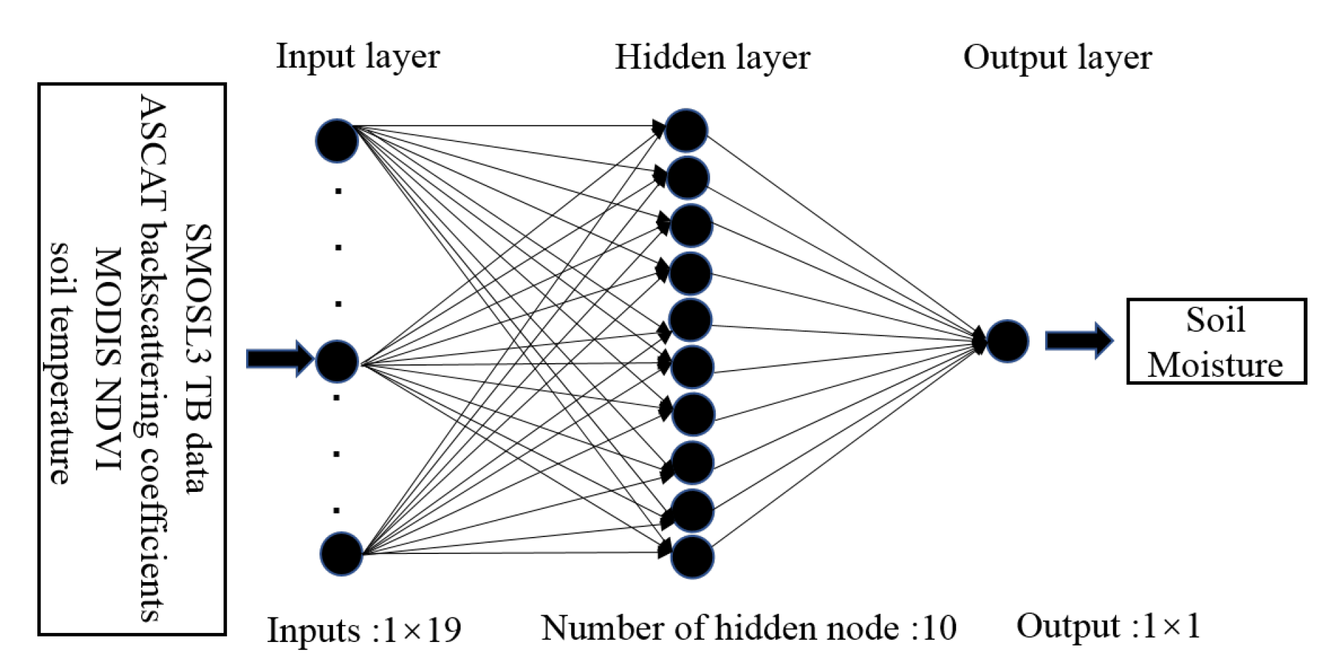
3.1. Neural Network
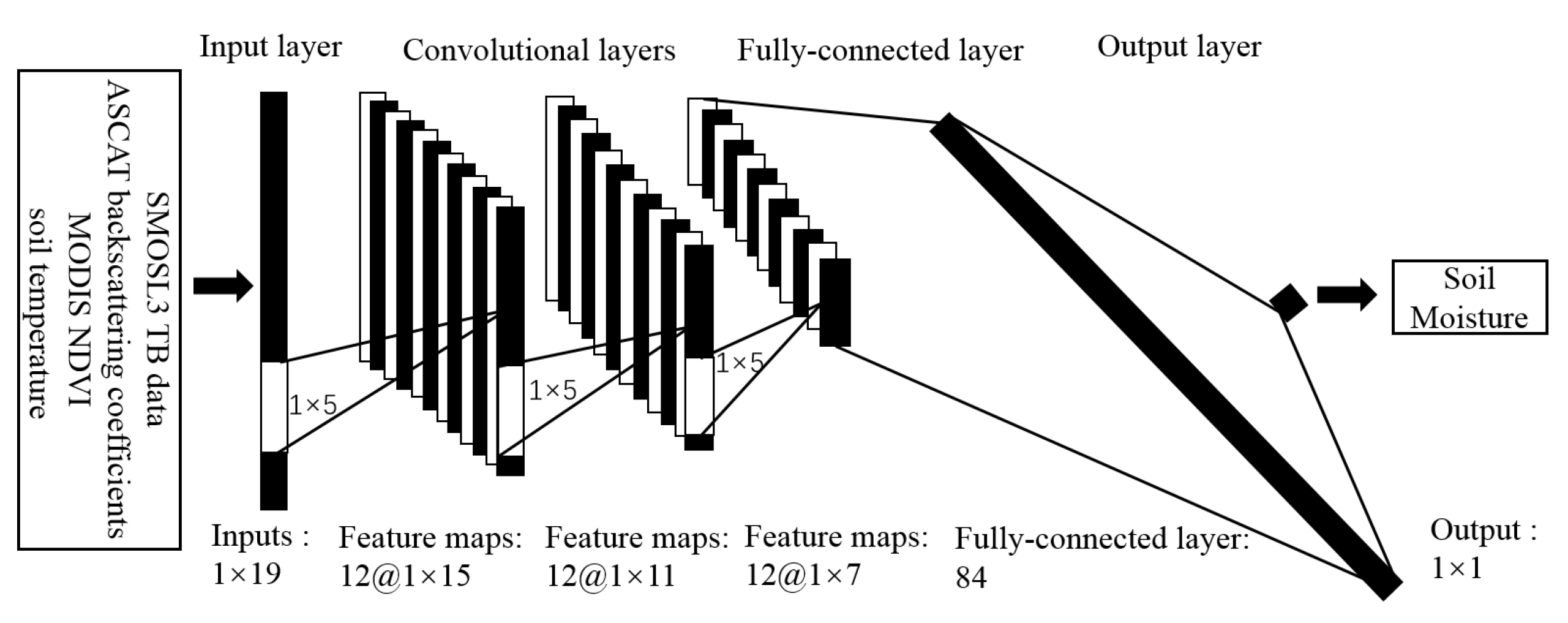
3.2. Deep Convolutional Neural Network
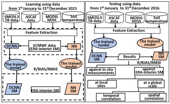
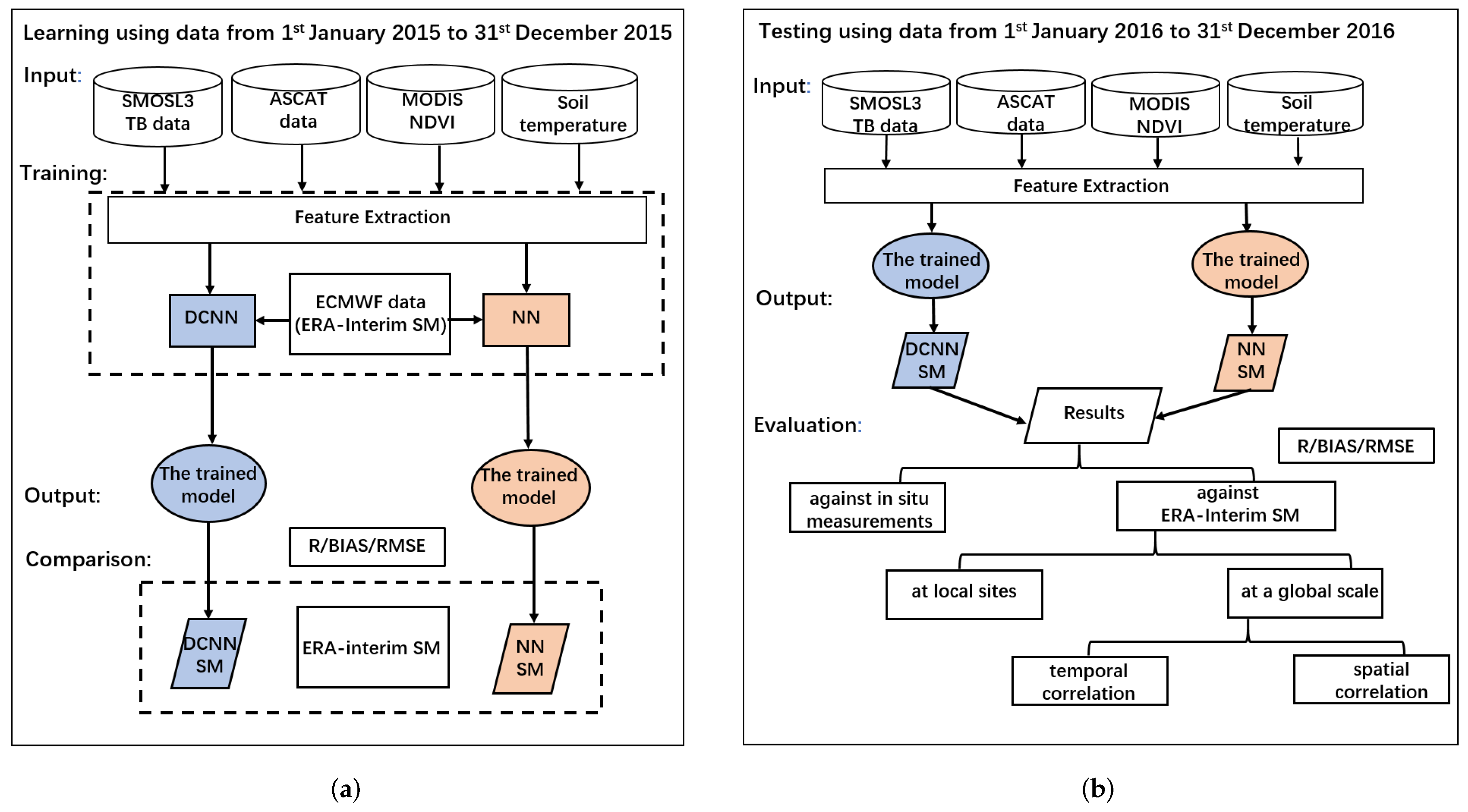
4. Experiments
4.1. Experimental Settings
4.2. Data Preprocessing
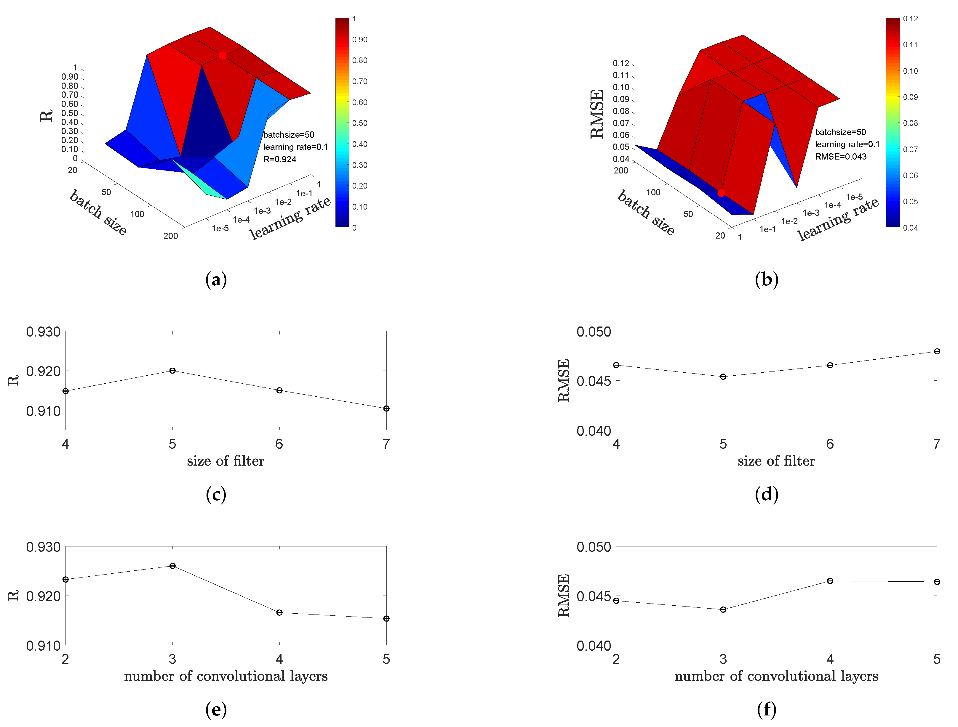
4.3. Hyperparameter Selection
4.4. Performance Comparison
5. Results
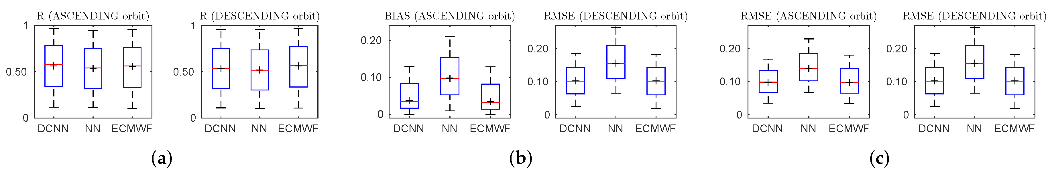
5.1. Comparison against In Situ Measurements
5.2. Temporal Correlation
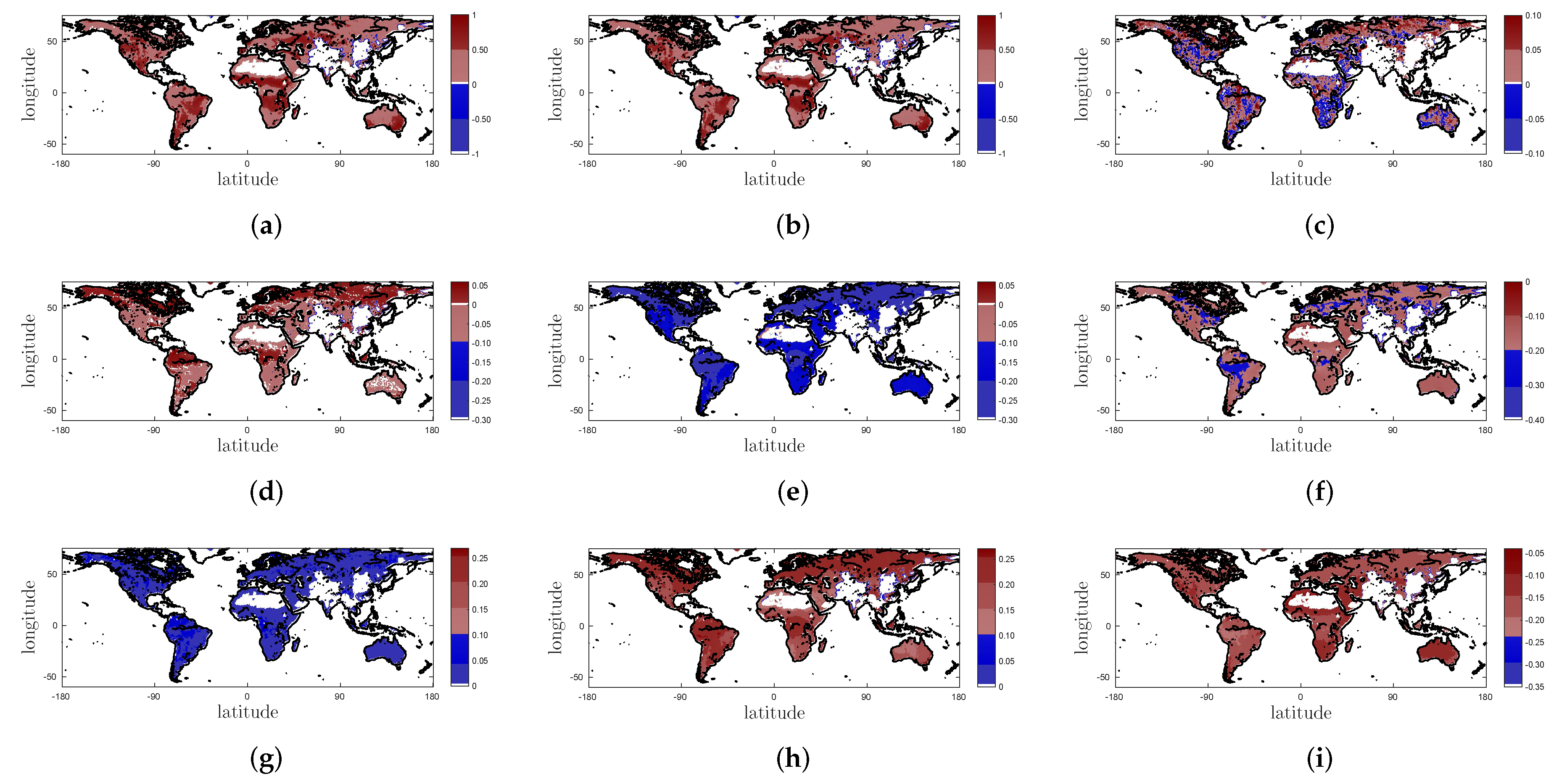
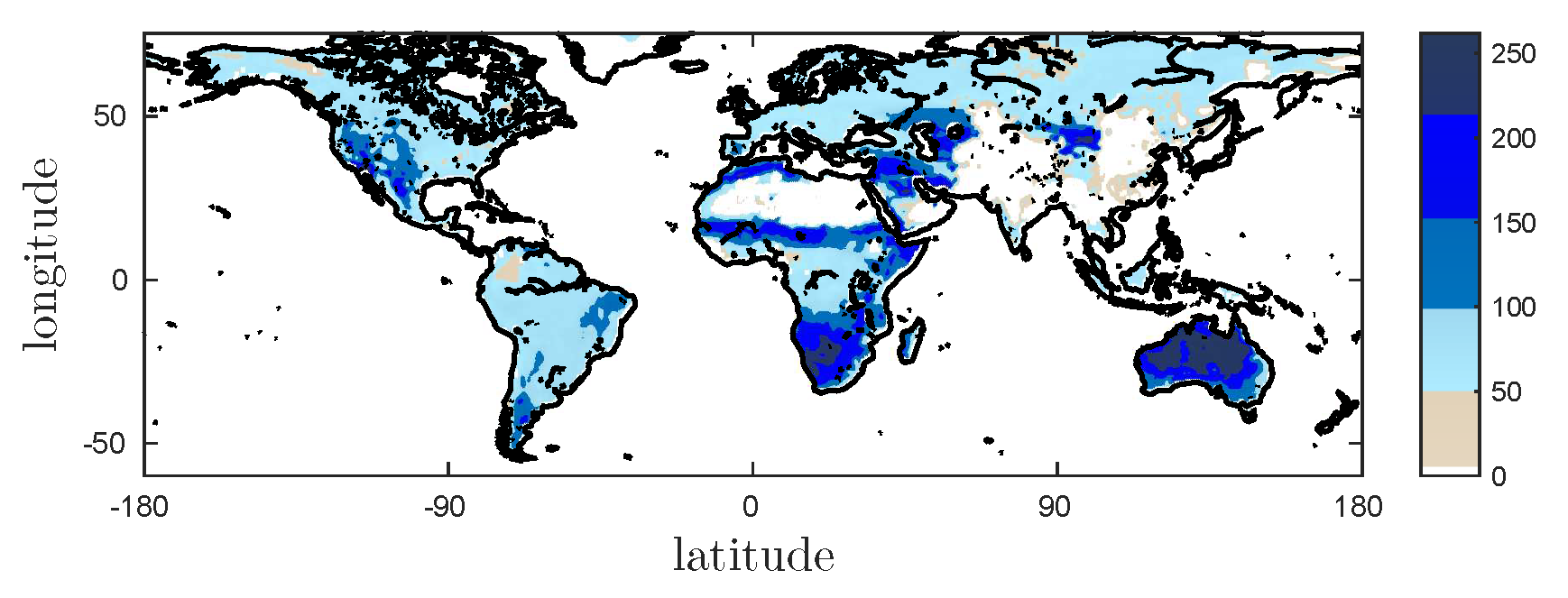
5.3. Spatial Correlation
6. Discussion
7. Conclusions
Author Contributions
Funding
Acknowledgments
Conflicts of Interest
References
- Secretariat, G. Implementation plan for the global observing system for climate in support of the UNFCCC (2010 Update). In Proceedings of the Conference of the Parties (COP), Copenhagen, Denmark, 7–19 December 2009. [Google Scholar]
- Gruber, A.; Paloscia, S.; Santi, E.; Notarnicola, C.; Pasolli, L.; Smolander, T.; Pulliainen, J.; Mittelbach, H.; Dorigo, W.; Wagner, W. Performance inter-comparison of soil moisture retrieval models for the MetOp-A ASCAT instrument. Geoscience and Remote Sensing Symposium (IGARSS). In Proceedings of the 2014 IEEE International Conference on Communications (ICC), Sydney, Australia, 10–14 June 2014; pp. 2455–2458. [Google Scholar]
- Hirschi, M.; Mueller, B.; Dorigo, W.; Seneviratne, S.I. Using remotely sensed soil moisture for land–Atmosphere coupling diagnostics: The role of surface vs. root-zone soil moisture variability. Remote Sens. Environ. 2014, 154, 246–252. [Google Scholar] [CrossRef]
- Kerr, Y.H.; Waldteufel, P.; Wigneron, J.P.; Delwart, S.; Cabot, F.; Boutin, J.; Escorihuela, M.J.; Font, J.; Reul, N.; Gruhier, C.; et al. The SMOS mission: New tool for monitoring key elements ofthe global water cycle. Proc. IEEE 2010, 98, 666–687. [Google Scholar] [CrossRef] [Green Version]
- Wagner, W.; Blöschl, G.; Pampaloni, P.; Calvet, J.C.; Bizzarri, B.; Wigneron, J.P.; Kerr, Y. Operational readiness of microwave remote sensing of soil moisture for hydrologic applications. Hydrol. Res. 2007, 38, 1–20. [Google Scholar] [CrossRef]
- Kerr, Y.H. Soil moisture from space: Where are we? Hydrogeol. J. 2007, 15, 117–120. [Google Scholar] [CrossRef]
- Liu, S.F.; Liou, Y.A.; Wang, W.J.; Wigneron, J.P.; Lee, J.B. Retrieval of crop biomass and soil moisture from measured 1.4 and 10.65 GHz brightness temperatures. IEEE Trans. Geosci. Remote Sens. 2002, 40, 1260–1268. [Google Scholar]
- Kerr, Y.H.; Waldteufel, P.; Wigneron, J.P.; Martinuzzi, J.; Font, J.; Berger, M. Soil moisture retrieval from space: The Soil Moisture and Ocean Salinity (SMOS) mission. IEEE Trans. Geosci. Remote Sens. 2001, 39, 1729–1735. [Google Scholar] [CrossRef]
- McMullan, K.; Brown, M.A.; Martín-Neira, M.; Rits, W.; Ekholm, S.; Marti, J.; Lemanczyk, J. SMOS: The payload. IEEE Trans. Geosci. Remote Sens. 2008, 46, 594–605. [Google Scholar] [CrossRef]
- Jackson, T.J.; Bindlish, R.; Cosh, M.H.; Zhao, T.; Starks, P.J.; Bosch, D.D.; Seyfried, M.; Moran, M.S.; Goodrich, D.C.; Kerr, Y.H.; et al. Validation of Soil Moisture and Ocean Salinity (SMOS) soil moisture over watershed networks in the US. IEEE Trans. Geosci. Remote Sens. 2012, 50, 1530–1543. [Google Scholar] [CrossRef] [Green Version]
- Kerr, Y.H.; Waldteufel, P.; Richaume, P.; Wigneron, J.P.; Ferrazzoli, P.; Mahmoodi, A.; Al Bitar, A.; Cabot, F.; Gruhier, C.; Juglea, S.E.; et al. The SMOS soil moisture retrieval algorithm. IEEE Trans. Geosci. Remote Sens. 2012, 50, 1384–1403. [Google Scholar] [CrossRef]
- Rodríguez-Fernández, N.J.; Aires, F.; Richaume, P.; Kerr, Y.H.; Prigent, C.; Kolassa, J.; Cabot, F.; Jiménez, C.; Mahmoodi, A.; Drusch, M. Soil moisture retrieval using neural networks: Application to SMOS. IEEE Trans. Geosci. Remote Sens. 2015, 53, 5991–6007. [Google Scholar] [CrossRef]
- Albergel, C.; De Rosnay, P.; Gruhier, C.; Muñoz-Sabater, J.; Hasenauer, S.; Isaksen, L.; Kerr, Y.; Wagner, W. Evaluation of remotely sensed and modelled soil moisture products using global ground-based in situ observations. Remote Sens. Environ. 2012, 118, 215–226. [Google Scholar] [CrossRef]
- Panciera, R.; Walker, J.P.; Kalma, J.D.; Kim, E.J.; Saleh, K.; Wigneron, J.P. Evaluation of the SMOS L-MEB passive microwave soil moisture retrieval algorithm. Remote Sens. Environ. 2009, 113, 435–444. [Google Scholar] [CrossRef]
- Santi, E.; Paloscia, S.; Pettinato, S.; Fontanelli, G. A prototype ANN based algorithm for the soil moisture retrieval from L-band in view of the incoming SMAP mission. In Proceedings of the 2014 13th Specialist Meeting on Microwave Radiometry and Remote Sensing of the Environment (MicroRad), Pasadena, CA, USA, 24–27 March 2014; pp. 5–9. [Google Scholar]
- Prigent, C.; Aires, F.; Rossow, W.B.; Robock, A. Sensitivity of satellite microwave and infrared observations to soil moisture at a global scale: Relationship of satellite observations to in situ soil moisture measurements. J. Geophys. Res. Atmos. 2005, 110. [Google Scholar] [CrossRef] [Green Version]
- Aires, F.; Prigent, C.; Rossow, W. Sensitivity of satellite microwave and infrared observations to soil moisture at a global scale: 2. Global statistical relationships. J. Geophys. Res. Atmos. 2005, 110. [Google Scholar] [CrossRef] [Green Version]
- Kolassa, J.; Aires, F.; Polcher, J.; Prigent, C.; Jimenez, C.; Pereira, J.M. Soil moisture retrieval from multi-instrument observations: Information content analysis and retrieval methodology. J. Geophys. Res. Atmos. 2013, 118, 4847–4859. [Google Scholar] [CrossRef] [Green Version]
- Rodríguez-Fernández, N.J.; Sabater, J.M.; Richaume, P.; de Rosnay, P.; Kerr, Y.H.; Albergel, C.; Drusch, M.; Mecklenburg, S. SMOS near-real-time soil moisture product: processor overview and first validation results. Hydrol. Earth Syst. Sci. 2017, 21, 5201–5216. [Google Scholar] [CrossRef] [Green Version]
- Liu, Q.; Zhou, F.; Hang, R.; Yuan, X. Bidirectional-Convolutional LSTM Based Spectral-Spatial Feature Learning for Hyperspectral Image Classification. Remote Sens. 2017, 9, 1330. [Google Scholar] [Green Version]
- Liu, Q.; Hang, R.; Song, H.; Li, Z. Learning Multiscale Deep Features for High-Resolution Satellite Image Scene Classification. IEEE Trans. Geosci. Remote Sens. 2018, 56, 117–126. [Google Scholar] [CrossRef]
- Berthon, L.; Mialon, A.; Bitar, A.A.; Cabot, F.; Kerr, Y. SMOS CATDS level 3 Soil Moisture products. In Proceedings of the EGU General Assembly Conference Abstracts, Vienna, Austria, 22–27 April 2012; Volume 14, p. 5456. [Google Scholar]
- Oliva, R.; Daganzo, E.; Kerr, Y.H.; Mecklenburg, S.; Nieto, S.; Richaume, P.; Gruhier, C. SMOS radio frequency interference scenario: Status and actions taken to improve the RFI environment in the 1400–1427-MHz passive band. IEEE Trans. Geosci. Remote Sens. 2012, 50, 1427–1439. [Google Scholar] [CrossRef] [Green Version]
- Kerr, Y.H.; Al-Yaari, A.; Rodriguez-Fernandez, N.; Parrens, M.; Molero, B.; Leroux, D.; Bircher, S.; Mahmoodi, A.; Mialon, A.; Richaume, P.; et al. Overview of SMOS performance in terms of global soil moisture monitoring after six years in operation. Remote Sens. Environ. 2016, 180, 40–63. [Google Scholar] [CrossRef]
- Gelsthorpe, R.; Schied, E.; Wilson, J. ASCAT-Metop’s advanced scatterometer. ESA Bull. 2000, 102, 19–27. [Google Scholar]
- Bartalis, Z.; Wagner, W.; Naeimi, V.; Hasenauer, S.; Scipal, K.; Bonekamp, H.; Figa, J.; Anderson, C. Initial soil moisture retrievals from the METOP-A Advanced Scatterometer (ASCAT). Geophys. Res. Lett. 2007, 34. [Google Scholar] [CrossRef] [Green Version]
- Brocca, L.; Hasenauer, S.; Lacava, T.; Melone, F.; Moramarco, T.; Wagner, W.; Dorigo, W.; Matgen, P.; Martínez-Fernández, J.; Llorens, P.; et al. Soil moisture estimation through ASCAT and AMSR-E sensors: An intercomparison and validation study across Europe. Remote Sens. Environ. 2011, 115, 3390–3408. [Google Scholar] [CrossRef]
- Wagner, W.; Lemoine, G.; Borgeaud, M.; Rott, H. A study of vegetation cover effects on ERS scatterometer data. IEEE Trans. Geosci. Remote Sens. 1999, 37, 938–948. [Google Scholar] [CrossRef]
- Lindsley, R.D.; Long, D.G. Enhanced-resolution reconstruction of ASCAT backscatter measurements. IEEE Trans. Geosci. Remote Sens. 2016, 54, 2589–2601. [Google Scholar] [CrossRef]
- Paloscia, S.; Pettinato, S.; Santi, E.; Notarnicola, C.; Pasolli, L.; Reppucci, A. Soil moisture mapping using Sentinel-1 images: Algorithm and preliminary validation. Remote Sens. Environ. 2013, 134, 234–248. [Google Scholar] [CrossRef]
- Berrisford, P.; Dee, D.; Poli, P.; Brugge, R.; Fielding, K.; Fuentes, M.; Kallberg, P.; Kobayashi, S.; Uppala, S.; Simmons, A. The ERA-Interim Archive Version 2.0; ERA Report Series 1; ECMWF: Shinfield Park, Reading, UK, 2011; 23p. [Google Scholar]
- Dee, D.P.; Uppala, S.M.; Simmons, A.J.; Berrisford, P.; Poli, P.; Kobayashi, S.; Andrae, U.; Balmaseda, M.A.; Balsamo, G.; Bauer, P.; et al. The ERA-Interim reanalysis: Configuration and performance of the data assimilation system. Q. J. R. Meteorol. Soc. 2011, 137, 553–597. [Google Scholar] [CrossRef]
- Balsamo, G.; Albergel, C.; Beljaars, A.; Boussetta, S.; Brun, E.; Cloke, H.; Dee, D.; Dutra, E.; Muñoz-Sabater, J.; Pappenberger, F.; et al. ERA-Interim/Land: A global land surface reanalysis data set. Hydrol. Earth Syst. Sci. 2015, 19, 389–407. [Google Scholar] [CrossRef]
- Zhou, J.; Wen, J.; Wang, X.; Jia, D.; Chen, J. Analysis of the Qinghai-Xizang Plateau monsoon evolution and its linkages with soil moisture. Remote Sens. 2016, 8, 493. [Google Scholar] [CrossRef]
- Viterbo, P.; Beljaars, A.C. An improved land surface parameterization scheme in the ECMWF model and its validation. J. Clim. 1995, 8, 2716–2748. [Google Scholar] [CrossRef]
- Viterbo, P.; Betts, A.K. Impact on ECMWF forecasts of changes to the albedo of the boreal forests in the presence of snow. J. Geophys. Res. Atmos. 1999, 104, 27803–27810. [Google Scholar] [CrossRef] [Green Version]
- Schaefer, G.L.; Cosh, M.H.; Jackson, T.J. The USDA natural resources conservation service soil climate analysis network (SCAN). J. Atmos. Ocean. Technol. 2007, 24, 2073–2077. [Google Scholar] [CrossRef]
- Al Bitar, A.; Leroux, D.; Kerr, Y.H.; Merlin, O.; Richaume, P.; Sahoo, A.; Wood, E.F. Evaluation of SMOS soil moisture products over continental US using the SCAN/SNOTEL network. IEEE Trans. Geosci. Remote Sens. 2012, 50, 1572–1586. [Google Scholar] [CrossRef] [Green Version]
- Kolassa, J.; Gentine, P.; Prigent, C.; Aires, F. Soil moisture retrieval from AMSR-E and ASCAT microwave observation synergy. Part 1: Satellite data analysis. Remote Sens. Environ. 2016, 173, 1–14. [Google Scholar] [CrossRef]
- Rumelhart, D.E.; Hinton, G.E.; Williams, R.J. Learning representations by back-propagating errors. Nature 1986, 323, 533–536. [Google Scholar] [CrossRef]
- Rumelhart, D.E.; Durbin, R.; Golden, R.; Chauvin, Y. Backpropagation: The basic theory. In Backpropagation: Theory, Architectures and Applications; Psychology Press: London, UK, 1995; pp. 1–34. [Google Scholar]
- Moré, J.J. The Levenberg-Marquardt algorithm: Implementation and theory. In Numerical Analysis; Springer: Berlin/Heidelberg, Germany, 1978; pp. 105–116. [Google Scholar]
- Scott, G.J.; England, M.R.; Starms, W.A.; Marcum, R.A.; Davis, C.H. Training deep convolutional neural networks for land–cover classification of high-resolution imagery. IEEE Geosci. Remote Sens. Lett. 2017, 14, 549–553. [Google Scholar] [CrossRef]
- Hu, F.; Xia, G.S.; Hu, J.; Zhang, L. Transferring deep convolutional neural networks for the scene classification of high-resolution remote sensing imagery. Remote Sens. 2015, 7, 14680–14707. [Google Scholar] [CrossRef]
- Castelluccio, M.; Poggi, G.; Sansone, C.; Verdoliva, L. Land use classification in remote sensing images by convolutional neural networks. arXiv 2015, arXiv:1508.00092. [Google Scholar]
- LeCun, Y.; Huang, F.J.; Bottou, L. Learning methods for generic object recognition with invariance to pose and lighting. In Proceedings of the 2004 IEEE Computer Society Conference on Computer Vision and Pattern Recognition Related Articles, Washington, DC, USA, 27 June–2 July 2004; IEEE: Piscataway, NJ, USA; Volume 2, pp. II–104. [Google Scholar]
- Abdel-Hamid, O.; Mohamed, A.-r.; Jiang, H.; Penn, G. Applying convolutional neural networks concepts to hybrid NN-HMM model for speech recognition. In Proceedings of the 2012 IEEE International Conference on Acoustics, Speech and Signal Processing, Kyoto, Japan, 25–30 March 2012; IEEE: Piscataway, NJ, USA, 2012; pp. 4277–4280. [Google Scholar]
- Lawrence, S.; Giles, C.L.; Tsoi, A.C.; Back, A.D. Face recognition: A convolutional neural-network approach. IEEE Trans. Neural Netw. 1997, 8, 98–113. [Google Scholar] [CrossRef] [PubMed]
- Cai, Z.; Fan, Q.; Feris, R.S.; Vasconcelos, N. A unified multi-scale deep convolutional neural network for fast object detection. In Proceedings of the 14th European Conference on Computer Vision, Amsterdam, The Netherlands, 8–16 October 2016; Springer: Berlin/Heidelberg, Germany, 2016; pp. 354–370. [Google Scholar]
- Maturana, D.; Scherer, S. Voxnet: A 3d convolutional neural network for real-time object recognition. In Proceedings of the 2015 IEEE/RSJ International Conference on Intelligent Robots and Systems (IROS), Hamburg, Germany, 28 September–2 October 2015; pp. 922–928. [Google Scholar]
- Szegedy, C.; Toshev, A.; Erhan, D. Deep neural networks for object detection. In Advances in Neural Information Processing Systems; NIPS Foundation: Montreal, CA, USA, 2013; pp. 2553–2561. [Google Scholar]


| ASCENDING Orbit | DESCENDING Orbit | |||||
|---|---|---|---|---|---|---|
| DCNN SM | NN SM | ERA-Interim SM | DCNN SM | NN SM | ERA-Interim SM | |
| MIN | 0.117 | 0.111 | 0.102 | 0.109 | 0.103 | 0.107 |
| MEAN | 0.564 | 0.531 | 0.556 | 0.530 | 0.517 | 0.562 |
| MEDIAN | 0.593 | 0.548 | 0.567 | 0.544 | 0.500 | 0.573 |
| MAX | 0.966 | 0.947 | 0.955 | 0.953 | 0.955 | 0.967 |
| MIN | 0.000 | 0.009 | 0.000 | 0.000 | 0.001 | 0.002 |
| MEAN | 0.036 | 0.097 | 0.035 | 0.037 | 0.107 | 0.040 |
| MEDIAN | 0.033 | 0.096 | 0.028 | 0.030 | 0.111 | 0.034 |
| MAX | 0.129 | 0.211 | 0.128 | 0.115 | 0.238 | 0.120 |
| MIN | 0.035 | 0.067 | 0.033 | 0.025 | 0.065 | 0.019 |
| MEAN | 0.099 | 0.140 | 0.098 | 0.102 | 0.156 | 0.102 |
| MEDIAN | 0.098 | 0.138 | 0.097 | 0.101 | 0.154 | 0.101 |
| MAX | 0.168 | 0.229 | 0.180 | 0.185 | 0.263 | 0.183 |
| ASCENDING Orbit | DESCENDING Orbit | |||
|---|---|---|---|---|
| DCNN SM | NN SM | DCNN SM | NN SM | |
| MIN | 0.635 | 0.606 | 0.573 | 0.515 |
| MEAN | 0.663 | 0.636 | 0.600 | 0.550 |
| MEDIAN | 0.672 | 0.644 | 0.599 | 0.550 |
| MAX | 0.682 | 0.656 | 0.617 | 0.565 |
| MIN | 0.009 | 0.090 | 0.000 | 0.102 |
| MEAN | 0.010 | 0.090 | 0.010 | 0.104 |
| MEDIAN | 0.011 | 0.094 | 0.011 | 0.104 |
| MAX | 0.011 | 0.096 | 0.022 | 0.106 |
| MIN | 0.035 | 0.108 | 0.035 | 0.119 |
| MEAN | 0.036 | 0.111 | 0.037 | 0.122 |
| MEDIAN | 0.036 | 0.111 | 0.037 | 0.122 |
| MAX | 0.037 | 0.112 | 0.038 | 0.124 |
| ASCENDING Orbit | DESCENDING Orbit | |||
|---|---|---|---|---|
| DCNN SM | NN SM | DCNN SM | NN SM | |
| R | 0.576 | 0.570 | 0.568 | 0.558 |
| 0.014 | 0.184 | 0.019 | 0.180 | |
| 0.036 | 0.199 | 0.040 | 0.196 | |
| ASCENDING Orbit | DESCENDING Orbit | |||
|---|---|---|---|---|
| DCNN SM | NN SM | DCNN SM | NN SM | |
| R | 0.927 | 0.924 | 0.926 | 0.922 |
| 0.006 | 0.006 | 0.009 | 0.009 | |
| 0.043 | 0.043 | 0.045 | 0.048 | |
© 2018 by the authors. Licensee MDPI, Basel, Switzerland. This article is an open access article distributed under the terms and conditions of the Creative Commons Attribution (CC BY) license (http://creativecommons.org/licenses/by/4.0/).
Share and Cite
Ge, L.; Hang, R.; Liu, Y.; Liu, Q. Comparing the Performance of Neural Network and Deep Convolutional Neural Network in Estimating Soil Moisture from Satellite Observations. Remote Sens. 2018, 10, 1327. https://doi.org/10.3390/rs10091327
Ge L, Hang R, Liu Y, Liu Q. Comparing the Performance of Neural Network and Deep Convolutional Neural Network in Estimating Soil Moisture from Satellite Observations. Remote Sensing. 2018; 10(9):1327. https://doi.org/10.3390/rs10091327
Chicago/Turabian StyleGe, Lingling, Renlong Hang, Yi Liu, and Qingshan Liu. 2018. "Comparing the Performance of Neural Network and Deep Convolutional Neural Network in Estimating Soil Moisture from Satellite Observations" Remote Sensing 10, no. 9: 1327. https://doi.org/10.3390/rs10091327
APA StyleGe, L., Hang, R., Liu, Y., & Liu, Q. (2018). Comparing the Performance of Neural Network and Deep Convolutional Neural Network in Estimating Soil Moisture from Satellite Observations. Remote Sensing, 10(9), 1327. https://doi.org/10.3390/rs10091327