Road Centerline Extraction from Very-High-Resolution Aerial Image and LiDAR Data Based on Road Connectivity

1
Department of Geography and Planning, Sun Yat-Sen University, Guangzhou 510275, China
2
School of Geographical Sciences, Guangzhou University, Guangzhou 510006, China
3
Guangzhou Urban Planning and Design Survey Research Institute, Guangzhou 510060, China
*
Author to whom correspondence should be addressed.
Remote Sens. 2018, 10(8), 1284; https://doi.org/10.3390/rs10081284
Submission received: 31 July 2018
/
Revised: 31 July 2018
/
Accepted: 10 August 2018
/
Published: 15 August 2018
(This article belongs to the Section Remote Sensing Image Processing)
Abstract
:The road networks provide key information for a broad range of applications such as urban planning, urban management, and navigation. The fast-developing technology of remote sensing that acquires high-resolution observational data of the land surface offers opportunities for automatic extraction of road networks. However, the road networks extracted from remote sensing images are likely affected by shadows and trees, making the road map irregular and inaccurate. This research aims to improve the extraction of road centerlines using both very-high-resolution (VHR) aerial images and light detection and ranging (LiDAR) by accounting for road connectivity. The proposed method first applies the fractal net evolution approach (FNEA) to segment remote sensing images into image objects and then classifies image objects using the machine learning classifier, random forest. A post-processing approach based on the minimum area bounding rectangle (MABR) is proposed and a structure feature index is adopted to obtain the complete road networks. Finally, a multistep approach, that is, morphology thinning, Harris corner detection, and least square fitting (MHL) approach, is designed to accurately extract the road centerlines from the complex road networks. The proposed method is applied to three datasets, including the New York dataset obtained from the object identification dataset, the Vaihingen dataset obtained from the International Society for Photogrammetry and Remote Sensing (ISPRS) 2D semantic labelling benchmark and Guangzhou dataset. Compared with two state-of-the-art methods, the proposed method can obtain the highest completeness, correctness, and quality for the three datasets. The experiment results show that the proposed method is an efficient solution for extracting road centerlines in complex scenes from VHR aerial images and light detection and ranging (LiDAR) data.
1. Introduction
The road network is the backbone of the city [1] and plays an essential role in many application fields, such as city planning, navigation, and transportation [2,3,4]. Conventional methods to obtain the road network require extensive surveying fieldworks and are often time-consuming and costly [5]. The fast-developing technology of remote sensing offers abundant and continuous observations of the land surface, making it an attractive data source for producing road maps [6].
Extensive efforts have been made to extract information on the road network from optical remote sensing images [7,8]. The spatial resolution of the remote sensing images needs to be sufficiently high to allow road recognition [9]. Roads in the very-high-resolution (VHR) images are locally homogeneous and have elongated shapes with specific width [3,10]. Given the above characteristics, some studies designed the detectors of points and lines to extract road networks. For example, Hu et al. [11] designed a spoke wheel operator for quantifying angular texture feature of pixels and detecting road pixels. Liu et al. [10] first detected road edges from remote sensing data to extract the road networks. Shi et al. [12] detected road segments by the template matching method and then generated a connected road network. In addition, the image classification is another common solution to road extraction from optical remote sensing images [13,14,15,16]. The basic idea of the solution is first to classify remote sensing images into binary road and non-road groups and then post-process the road groups based on the structural characteristics and contextual features to obtain the road network [15,17]. In general, although various methods for road network extraction have been proposed, it is still a challenging task to extract complete and accurate road networks from VHR images in complex scenes because of the interferences of trees, shadows and non-road impervious surface (such as buildings and parking lots) [4].
Studies have also tried to extract the road networks from the light detection and ranging (LiDAR) data [18,19,20,21,22]. Airborne LiDAR is a new surveying technology that could provide three-dimensional information of surface objects, which can be used to effectively distinguish roads from buildings [23]. In addition, the multiple echoes of airborne LiDAR can weaken the influence of tree obscuration on road extraction [24]. Extracting road networks from the airborne LiDAR data typically consists of two steps: road point clouds identification and road network construction [18]. The intensity information of the LiDAR point clouds is often used for extracting the road point clouds. For example, Clode et al. [25] extracted road points by setting an empirical threshold of intensities. To reduce the subjectivity of threshold determination, Choi et al. [19] set the intensity threshold based on the mean and variance of the intensities of the road points, which are selected by reference to VHR images. Xu et al. [20] determined the intensity threshold based on the histogram. For road network construction, Hu et al. [21] first extracted road center points by clustering the road points using the mean shift algorithm and then generated road centerlines using a weighted Hough transform. Hui et al. [22] derived road centerlines by first rasterizing the road point clouds and then extracting the road centerlines using a hierarchical fusion and optimization algorithm. While the current studies have demonstrated the potential of airborne LiDAR for the application of road extraction, it is still difficult to use the LiDAR data alone without the spectral information for road extraction because the non-road impervious surface is easily misidentified as roads [18,20,26].
To overcome the disadvantage of using single-source remote sensing data, recent studies try to extract road networks by combining VHR images with the LiDAR data [27,28]. These methods can be divided into two categories. One is to use the LiDAR data as the primary data and the VHR images as the supplemental data. In this category of methods, the VHR images are usually used to assist the identification of road point clouds. For example, Liu et al. [27] fused the LiDAR data with Red-Green-Blue (RGB) images to obtain point clouds with multispectral information and derive road networks from the fused data. Hu et al. [29] extracted road points from ground points by combining the contextual information derived from the aerial images and then obtained road network from road points using the iterative Hough transform algorithm. The other method is to use VHR images as the primary data and the LiDAR data as the supplemental data. In this category of methods, the LiDAR data is often first converted into digital surface model (DSM) and normalized DSM (nDSM) and then used analogously as a spectral band. For example, Sameen et al. [28] first derived nDSM from the LiDAR data, then extracted the road networks combining VHR images with nDSM by a fuzzy object-based analysis. Grote et al. [30] obtained the road networks by integrating the intensity and DSM derived from LiDAR data and the spectral features using a pixel-based classification method. In general, although some methods have been proposed, the problem of removing obscuration effects of trees and shadows on road extraction has not been solved well [21].
Road centerlines is another effective representation of the roads and can clearly show the road topology and accurately locate the position of the road [31]. The morphological thinning is a common method for road centerline extraction [32,33,34], but the accuracy of road centerlines extracted by the method is relatively low [32,33]. To improve road centerlines extraction, Zhang et al. [35] proposed a road centerline extraction method based on the random transform. Poullis et al. [36] used the Hough transform algorithm to extract road centerlines. Although these methods perform well for straight road segments, they are not suitable for the complex road networks. To extract the road centerlines from the complex road networks, Shi et al. [33] first decomposed the road network into unconnected road segments and then extracted the road centerline for each road segment using a locally weighted regression method. Finally, all the isolated road centerlines were further linked to form the road centerline network. Although the method solves the problem of road centerline extraction of multi-branch road networks, the road centerline extraction effect is still poor for the curve road segments.
In order to improve the accuracy of road centerline extraction under complex scenes, this paper proposes a novel road centerline extraction method combining VHR images with LiDAR data. The main contributions of the research are to (1) develop an interference processing approach based on MABR to eliminate the negative effects of shadows, trees, and cars on the road network; and (2) propose a road centerline extraction approach to obtain regular and complete road centerline networks from complex road networks. The remainder of this paper is organized as follows. Section 2 introduces the study materials and data preprocessing. Section 3 describes the principle and process of the proposed method in detail. The road centerline extraction results of three datasets are given in Section 4. Section 5 discusses the effectiveness and uncertainty of the proposed method. Finally, the conclusion is presented in Section 6.
2. Study Materials
In this study, three datasets are chosen to assess the effectiveness and adaptability of the proposed method.
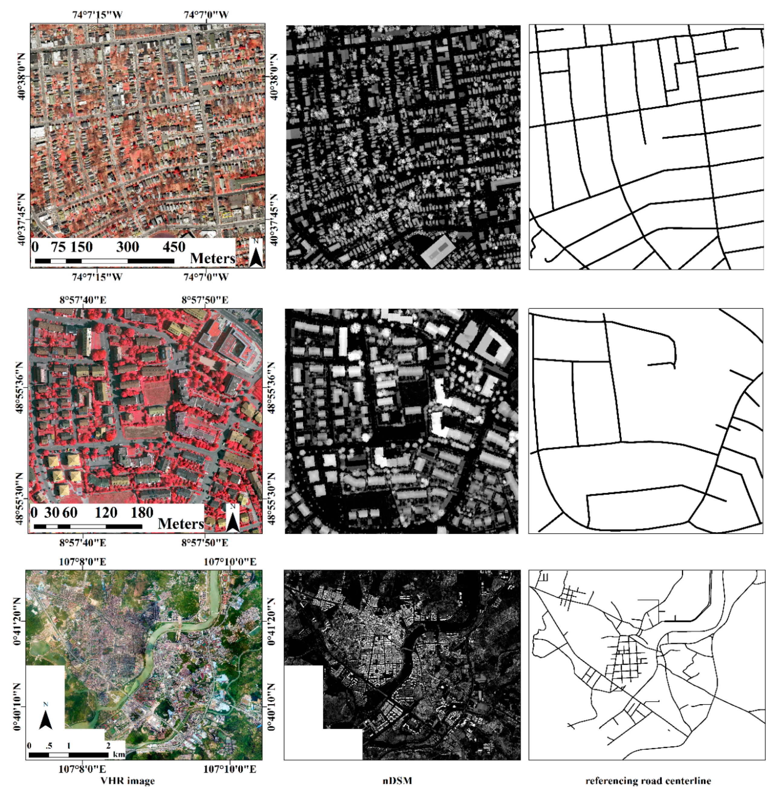
The first dataset shown in the first row of Figure 1 is located in New York; therefore, it is called the New York dataset in this paper. It comes from the object identification dataset [37], which was collected in 2014 and included both VHR images and airborne LiDAR data. The VHR images have a spatial resolution of 15 cm and include four channels of the red, green, blue, and near-infrared bands. The spatial size of the VHR image used in this paper is 5200 × 5000 pixels. The airborne LiDAR data is provided as point clouds and the density is approximately 5 points/m2. In this dataset, roads have similar spectral signatures with other impervious surface (such as the parking lots and buildings) and the road is often covered and sheltered by shadows, trees, and cars.
The second dataset is the Vaihingen dataset [38], which is obtained from the ISPRS 2D semantic labelling benchmark and includes both VHR images and airborne LiDAR data. It is shown in the second row of Figure 1. The VHR images consist of the red, green, and near-infrared bands with a spatial resolution of 9 cm. The image size used is 4300 × 4200 pixels. The airborne LiDAR data was captured with the Leica ALS50 system, and its average point density is 4 points/m2. Roads in the Vaihingen dataset vary in widths and shapes, and are severely influenced by shadows, trees, and cars.
The third dataset is the Guangzhou dataset and is shown in the third row of Figure 1. It covers 28.8 km2 for Conghua district, Guangzhou city, and is used to access the effectiveness of the proposed method for large-scale road extraction. The Guangzhou dataset consists of VHR images and airborne LiDAR data, and was collected using the Y-5 fixed wing aircraft in 2015. The VHR image has a spatial resolution of 0.5 m, including three channels of red, green, and blue, and was collected using tianbao AC IC180 digital camera. The airborne LiDAR data was captured with the Trimble Harrier68i system, and its average point density is 4.95 points/m2.
The airborne LiDAR point clouds are preprocessed into normalized digital surface model (nDSM) for subsequent analysis. The LiDAR point clouds are first used to derive the digital surface model (DSM) and then classified into ground and non-ground points by the multidirectional ground filtering algorithm [39]. The digital terrain model (DTM) was simply generated based on the ground points. nDSM that could describe the height of the objects aboveground is simply derived by the difference between DSM and DTM.
Road maps of the three experiment areas are downloaded from the OpenStreetMap (OSM) website [40] and rectified as the reference data.
3. Methodology
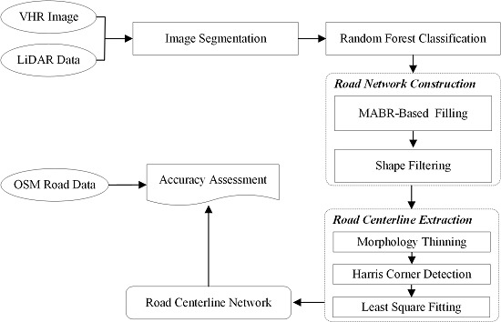
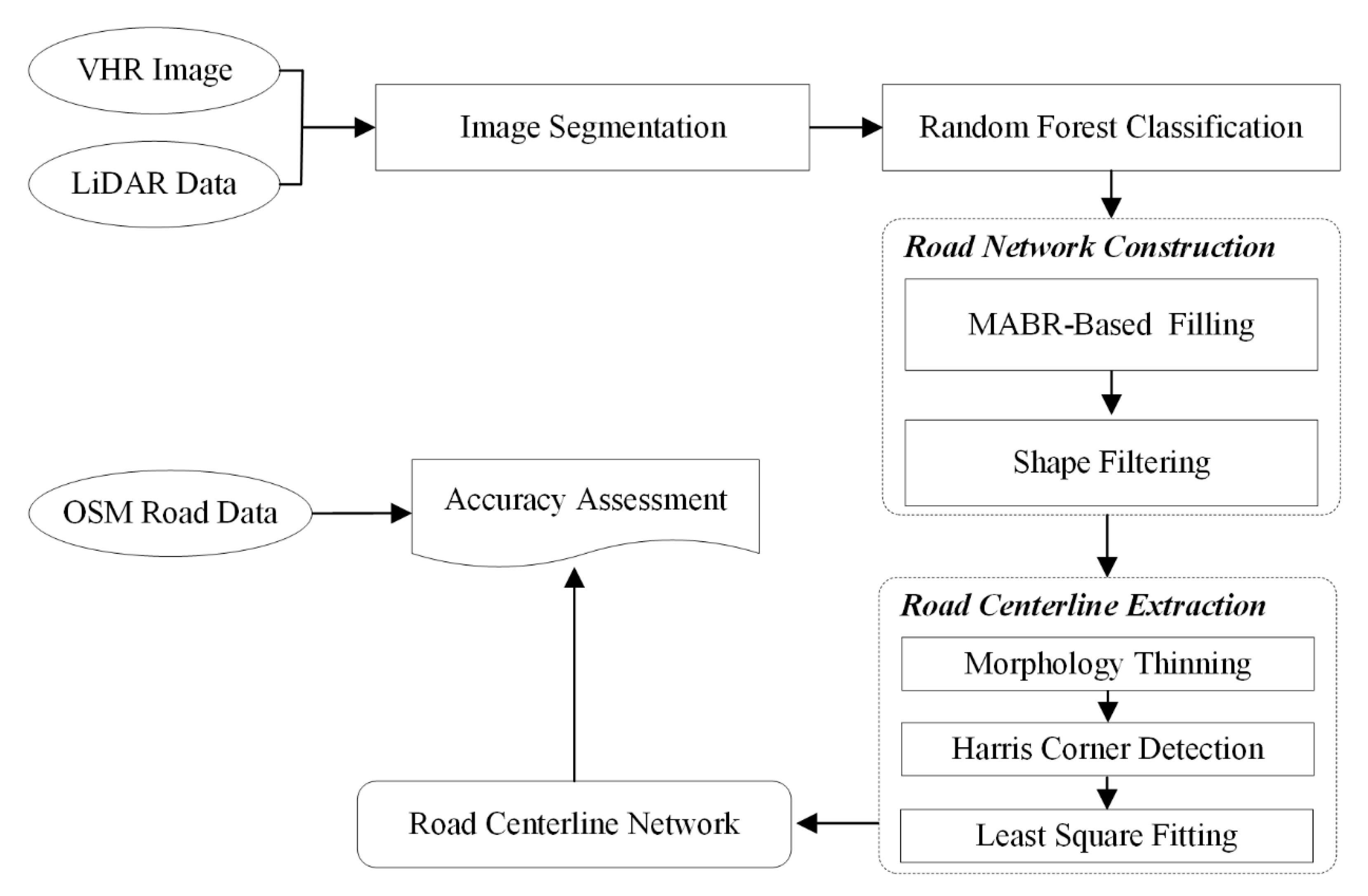
Figure 2 shows the workflow of the proposed method, which mainly involves the following steps: (1) segment the fused data of the VHR image and nDSM into image objects using the fractal net evolution approach (FNEA) [41]; (2) classify the image objects using the random forest classifier [42] based on the spectral, textural, and structural information; (3) generate road network by first applying a filling approach based on the minimum area bounding rectangle (MABR) [2] and then removing the false road segments by shape filtering based on the skeleton-based object linearity index (SOLI) [3]; (4) extract the road centerline network using a multistep approach, which mainly includes three processing steps, namely morphology thinning [34], Harris corner detection [43], and least square fitting [31], so it is called the MHL approach for short.
3.1. Image Segmentation
Image segmentation, a procedure that partitions an image into disjoint homogeneous segments, is one crucial step to perform object-based image analysis (OBIA) [44,45]. This study adopts FNEA [15,45,46], a bottom-up region-merging technique, to segment the fused data of the VHR images and nDSM. FNEA first starts from individual pixels to group pixels sharing similarities in spectral into objects and then merges every two adjacent objects iteratively until the fusion factor (f) reaches a scale parameter (T). Many studies have shown that the scale parameter (T) has an important influence on OBIA [44,47,48]. Thus, we will discuss the influence of T on road centerline extraction in detail in Section 5. The fusion factor f is defined as follows:
where and are the weights of the spectral and shape heterogeneities, respectively. In the three datasets of this paper, they are empirically set as 0.8 and 0.2, respectively; and are the differences of spectral and shape heterogeneity, respectively, between before and after object merging.
where B is the number of bands used in image segmentation; is the weight of band b (1 ≤ b ≤ B); , , and are the number of pixels in the merged object, object 1, and object 2, respectively; and , , and represent the corresponding standard deviations.
where and are the compactness and smoothness heterogeneities, respectively; and and are the corresponding weights, which are set as 0.4 and 0.6, respectively.
3.2. Random Forest Classification
This study applies the machine learning method, random forest, to classify the objects derived from the fused images into the classes of road, shadow, tree, car, building, and bare groups. The random forest classifier designed by Breiman [42] consists of a number of tree classifiers that are trained independently using a random feature subset sampled from the object feature sets and cast the votes to determine the class of the objects. The prediction of the object class can be expressed as the vote of all tree classifiers as follows:
where is the class for the object x; is the class for the object x based on the tree classifier i; K is the number of tree classifiers; Y represents the output variable; and I denotes an indicative function.
The random forest classifier requires defining two parameters, including the number of tree classifiers k and the number of features within the feature subset m [42,49]. The out-of-bag (OOB) errors are commonly used to evaluate the accuracy of the random forest classifier. As the number of tree classifiers increases, OOB errors gradually decrease to a certain level and the computation burden of the entire classification process increases [42]. To obtain sufficient classification accuracy with acceptable computation cost, k is set as the number of tree classifiers when the OOB error starts to converge [50]. By trial and error, OOB error has converged when k is set to 200 in the three datasets in this study. The number of features within the feature subset is usually set as one-third or square root of the total feature numbers [51] and is set in this study as the square root of the total feature number.
The features for each image object used in the random forest classifier include the spectral, elevation, texture, structural, and index features. The spectral feature used is derived as the average spectral value of pixels within the corresponding object as follows:
where is the spectral feature of object i in band b; and is the spectral value of pixel p in the corresponding band.
The elevation feature is useful to classify objects with different heights [47]. The elevation features used in this study include the elevation mean and the elevation variance as follows:
where EM is the elevation mean; EV is the the elevation variance; and is the nDSM value of pixel p.
The texture features that describe the spatial distribution of pixels within an object are useful for distinguishing among artificial objects [52]. The texture features are derived based on the gray-level co-occurrence matrix (GLCM) [51,53], which describes the local probability statistics tabulation of the occurrence of pixel gray level combinations. Both homogeneity (HOM) and entropy (ENT) are used to quantify the spectral heterogeneity of an object as follows:
where L is the number of gray levels; and is the value at cell (a, b) in the GLCM derived from object i.
Because roads in the VHR images have specific structural characteristics like elongated shapes and large curvatures [3,10], the structural feature is useful for road extraction from the VHR images. The metric of density is used to describe structural characteristics of objects:
where denotes the density; is the area of object i; and are the variance of the X coordinated and Y coordinated pixels, respectively, within object i.
The widely used vegetation index, normalized difference vegetation index (NDVI), is used to distinguish between vegetation and non-vegetation:
where and are the the average spectral value of object i in the near-infrared band and the red band, respectively.
3.3. Road Network Construction
3.3.1. MABR-Based FILLING
The road segments extracted by classification are often discontinuous. The main reasons causing the discontinuities of road segments include the following: (1) non-ground objects, such as trees and buildings, cast shadows on the road, which changes the spectral characteristics of road segments covered, and leads to the road segments being misclassified as shadows; (2) some road segments are shielded by trees on both sides of the road, which causes the road segments to be mistaken as trees. Thus, there is a significant adjacency relationship between the road segments and interference objects leading to the discontinuity of the road segment.
In order to link the discrete road segments and obtain a complete road network, road patches incorrectly classified as shadows and trees must be modified to road. Using the external rectangle of valid boundary pixels that refer to the boundary pixels of the interference object adjacent to the road segments is an effective method to approximatively represent the road patch. In general, the external rectangle includes minimum bounding rectangle (MBR) [54] and minimum area bounding rectangle (MABR) [2]. Compared with the MBR, the MABR can represent the road patch more accurately. Thus, this study uses the MABR of the valid boundary pixels to approximatively represent the road patch. The construction of the MABR was proposed by Wang [2]. The MBR of the valid boundary pixels is first created and used as a search rectangle and then the search rectangle is rotated around the centroid of the valid boundary pixels at a regular angle interval angle of 2°. The search rectangle with the smallest area is the MABR and used to approximatively represent the road patch.
Based on the above principles and methods, this study proposes a MABR-based filling approach to link the discrete road segments and obtain a complete road network. The detailed processing steps are given in Algorithm 1.
| Algorithm 1. The detailed processing steps of MABR-based filling approach. |
| Input: Object-based classification |
| Output: Complete road network |
| 1. For road, shadow and car classes, morphology opening is performed in turn to break small connections; |
| 2. Labal object-based classification by connected component analysis. Lshadow, Ltree and Lcar represent connected components of shadow, tree and car classes, respectively; |
| 3. Identify the adjacency relation between connected components. Ni is the number of road connected components adjacent to connected components i; |
| 4. For each Lshadow, Ltree and Lcar if (Ni ≥ 1) then extract valid boundary pixels and create the minimum area bounding rectangle (MABR). revise class of the pixels within the MABR as road. else continue end if |
| 5. Remove over-filling by taking building and bare classes as mask. |
3.3.2. Shape Filtering
After the filling processing, many false road segments, which are caused by misclassification and filling processing, still exist. Road segments are usually elongated structures with specific widths, making them distinguishable from the false road segments [3,11,33]. The skeleton-based object linearity index (SOLI) [3] is adopted to remove the false road segments:
where is the area of road segment b; and is the length of the road segment’s skeleton extracted using the morphology skeletonization. In order to remove the skeleton’s legs, morphology spurring is adopted and the parameter of processing times is set as twice maximum distance map value of object [3]; and are the minimum width value and maximum width value, respectively, of all roads within the network, which are obtained by external road-specific knowledge; and is the mean width of road segment b.
3.4. Road Centerline Extraction
Morphology thinning is a common approach to extract the road centerlines from the road segments [15,16,33]. It is both fast and easy to perform. However, the road centerlines extracted by the approach are unsmooth and have many spurs [33], especially in the complex road network with irregular boundaries. In order to obtain a smooth and accurate road centerline network from a complex road network, the least square fitting is adopt to post-process the initial road centerline network, which is extracted by morphology thinning in this study.
For each road centerline segment, the least square fitting can be expressed as follows:
where N is the number of pixels of the road centerline segment R; xi and yi represent the row number and the column number, respectively, of the road centerline pixel i; and is the column number of pixel i after fitting.
The initial road centerline network is usually complex and has many branches. Hence, least square fitting cannot be directly used to post-process the initial road centerline network. In order to solve the problem, the Harris corner detection approach [43,55] is used to decompose the initial road centerline network into the road centerline segment. The approach recognizes corner points according to the average gray change, which is calculated by moving a local windows in different directions and can be expressed as follows:
where E(x, y) represents the average gray change in the coordinate (x, y); is the local windows; and and represent the partial derivatives of the image in the s direction and the t direction, respectively. After the average change calculated, a threshold (TH) is set to extract corner points. When the average gray change of a pixel is greater than the threshold, the pixel is identified as a corner point. The threshold is set to 0.33 in the study.
The road centerline extraction approach proposed synthesizes the morphology thinning, the Harris corner detection, and the least square fitting, so it is called the MHL approach for short. Algorithm 2 shows its detailed processing steps.
| Algorithm 2. Road centerline extraction by the MHL approach. |
| Input: Complex road network |
| Output: Accurate road centerline network |
| 1. Extract the initial road centerline network by the morphology thinning; |
| 2. Decompose the initial road centerline network into the road centerline segment using the Harris corner detection. |
| 3. Link road centerline segments with similar direction and spatial neighborhood; |
| 4. Remove short road centralline segments whose length is less than the average road width; |
| 5. Fitting each road centerline segment using the least square fitting. |
3.5. Method Comparison
To understand the robustness of the proposed method based on comparative studies, two methods from the work of Huang [15] and Miao [32] are implemented to extract the road centerline network of the two experimental areas. The method proposed by Huang et al. (2009) takes a common strategy for road centerline extraction, which first conducts a multiscale segmentation and then classifies the image objects at each scale based on spectral-structural features and support vector machines. Finally, the road information for different scales is integrated and the morphology thinning is adopted to extract the road centerline network [15]. The method proposed by Miao et al. (2016) is a novel road centerline extraction method, which first extracts road segments using two different method, including expectation maximization clustering and linearness filter, and then obtains the road centerlines from the road segments using the RANdom SAmple Consensus. Finally, the discontinuous road centerlines are linked into a complete road centerline network by setting many information fusion rules [32].
3.6. Accuracy Assessment
The road data from OpenStreetMap (OSM) is applied as the reference data to assess the road centerline network extraction. Three common metrics, completeness, correctness, and quality, are adopt. To derive the evaluation metrics, a buffer with specified width is built for the extracted road centerline network [16,56]. The portion of reference road centerline network inside the buffer zone is called “matched reference” and the other portion is called “unmatched reference”. A same width buffer is then built around the reference road centerline network. The portion of road centerline network extracted inside the buffer zone is called “matched extraction”. Finally, the length of matched reference, unmatched reference, matched extraction, reference road centerline network, and extracted road centerline network are calculated. In this study, the buffer width of the three datasets are set as 25 pixels, 35 pixels, and 5 pixels, respectively.
Completeness is the ratio between matched reference with reference road centerline network as follows:
Correctness is the ratio between matched extraction with extracted road centerline network:
Quality is derived as follows:
4. Results
4.1. The New York Dataset
Figure 3 shows road network extraction for the New York dataset. It can be seen that (1) after image segmentation, the road objects present unique strip characteristics. However, due to the interference of shadows and trees, the road objects’ boundary is irregular (Figure 3a); (2) Because of the misclassification and interferences, some road segments are misclassified as shadows, trees, and cars, while some impervious surfaces are misclassified as roads (Figure 3b); (3) After interference filling, although the road network’s boundary is still irregular, many discrete road segments are connected, and the connectivity of the road network is significantly enhanced. However, there are still many false road segments (Figure 3c); (4) The shape filter based on the SOLI can remove the false road segments, and road networks can be well superimposed on the VHR image (Figure 3d). In general, there are a lot of mistakes in the road network extracted only by classification, and the MABR-based interference filling and the shape filtering can effectively eliminate the influence of interference factors on road extraction and obtain a complete road network from the classified image.
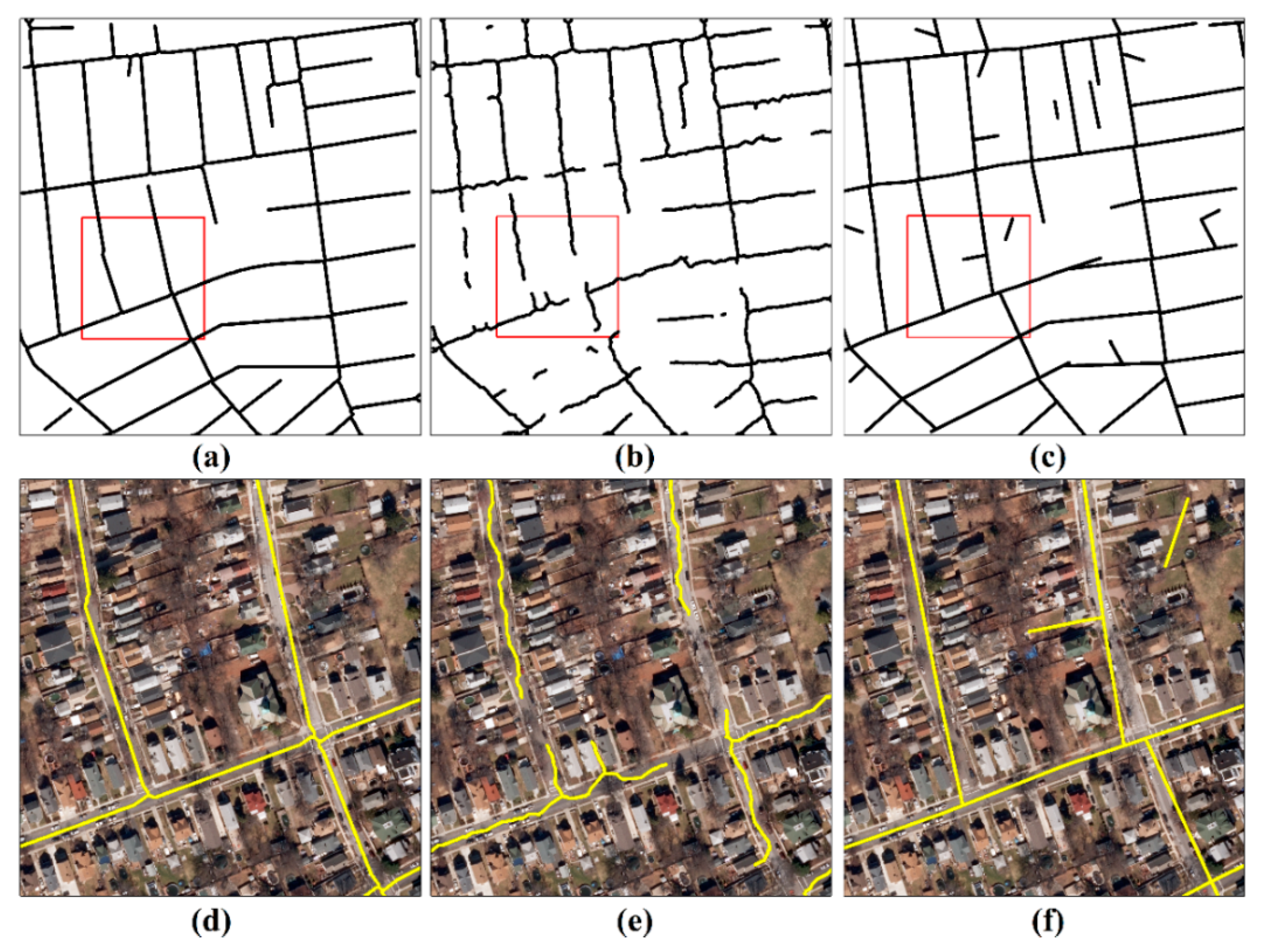
Figure 4 shows the road centerline network extraction of different methods for New York dataset. For this dataset, all the three methods could correctly extract most of the road segments. However, the road centerline network obtained by Huang’s method (Figure 4b) is discontinuous with many gaps in between road centerlines. The road centerline network obtained by Miao’s method (Figure 4c) has many false road centerline segments. Compared with Huang’s method and Miao’s method, the road centerline network obtained by the proposed method (Figure 4a) is both complete and regular. The road centerlines marked with red rectangle are overlaid on the false-color composite image as shown with details in Figure 4d–f. It is clear that the road centerline extraction of the proposed method can be better superimposed on the VHR image (Figure 4d), whereas one of Huang’s methods has many discontinuities where the road is shaded by trees (Figure 4e), and the one of Miao’s methods has many false road centerline segments, as well as low position accuracy, especially in curved road segments (Figure 4f). Overall, the visual comparison of different road centerline extraction illustrates the advantages of the proposed method in road centerline extraction for a complex scene.
Table 1 shows the quantitative assessment of road centerline extraction of different methods for the New York dataset. It can be seen that Huang’s method achieves relatively higher correctness, but the completeness and the quality are the lowest, indicating that the road centerline network extracted by classification method has high position accuracy, but there are also many omissions. Miao’s method can balance commissions and omissions, and the completeness and the correctness are close and both of them are greater than 0.85. However, the accuracy is still low, so it is difficult to meet the accuracy requirements of production application. Compared with Huang’s method and Miao’s method, the road centerline network extracted by the proposed method has the highest completeness, correctness, and quality value, which indicates that the proposed method can effectively balance between commissions and omissions, and improve the accuracy of the road network extraction.
4.2. The Vaihingen Dataset
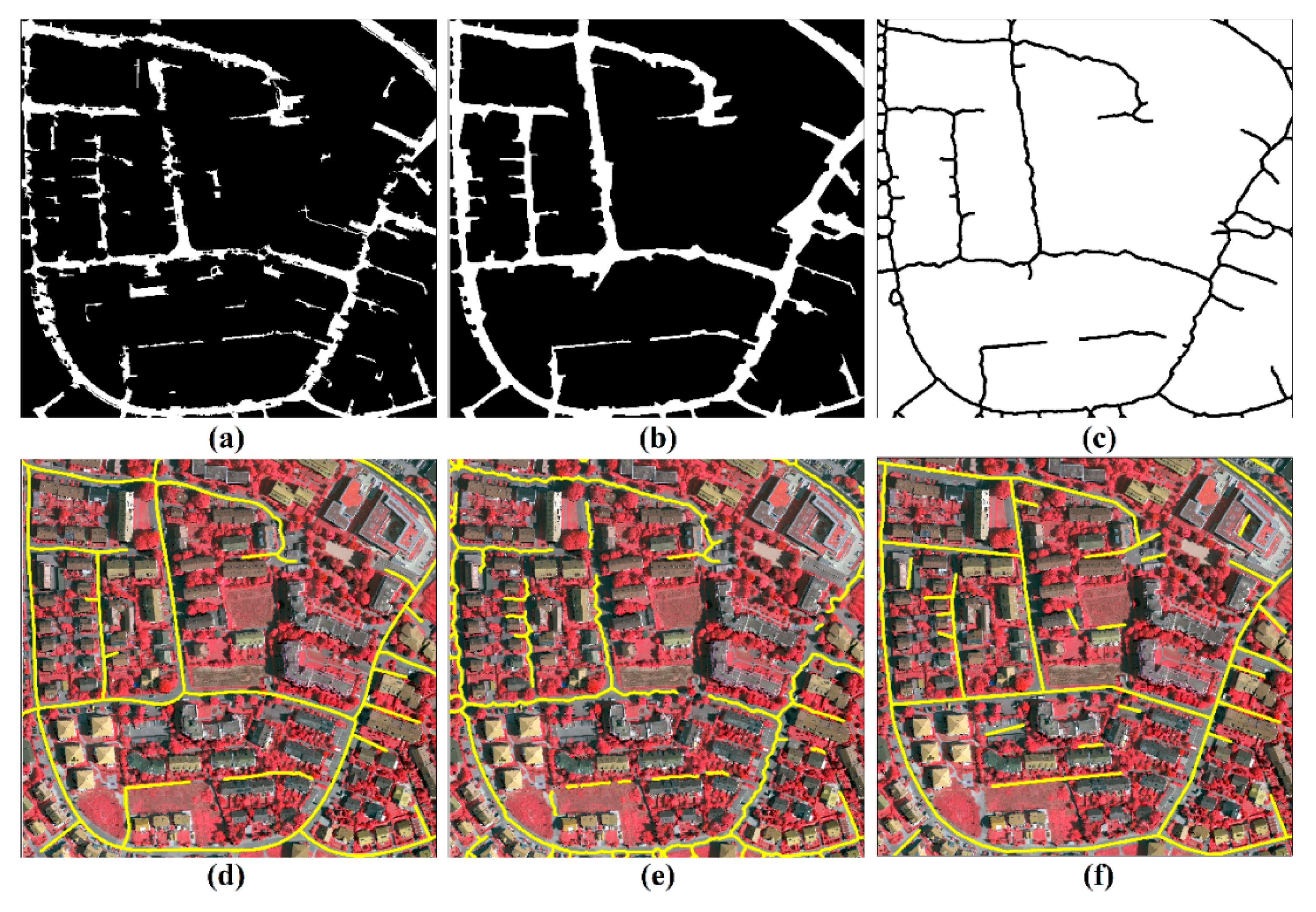
Figure 5 shows the road centerline network extraction for Vaihingen dataset. Initial road network (Figure 5a) is extracted by object-based classification. It can be seen that the initial road network is discontinuous and there are many false road segments. In order to obtain a complete and accurate road network, the initial road network is post-processed by the MABR-based interference filling and the shape filtering. Figure 5b shows the road network after post processing. Compared with Figure 5a, isolate road segments are linked and many false road segments are removed in Figure 5b. Figure 5c,d show the road centerline network extracted by the morphological thinning and the MHL approach, respectively. By comparison, the road centerline network extracted by the MHL approach is smooth and many short branches are removed. Figure 5e,f show the road centerline network extracted by Huang’s method and Miao’s method, respectively. It can be found that the road centerline network extracted by Huang’s method has a large number of discontinuous and short branches, and one extracted by Miao’s method is regular, but many non-road impervious surface are incorrectly detected as road. Overall, all three methods could correctly extract the roads with large width, however, the road centerline extraction results of the three methods are poor for narrow road segments with a large proportion of shadow obstructing.
Table 2 shows the quantitative assessment of road centerline extraction of different methods for the Vaihingen dataset. The similar conclusion can be obtained from the Vaihingen dataset. Compared with Huang’s method and Miao’s method, the proposed method can also achieve the highest completeness, correctness, and quality value in the Vaihingen dataset.
4.3. The Guangzhou Dataset
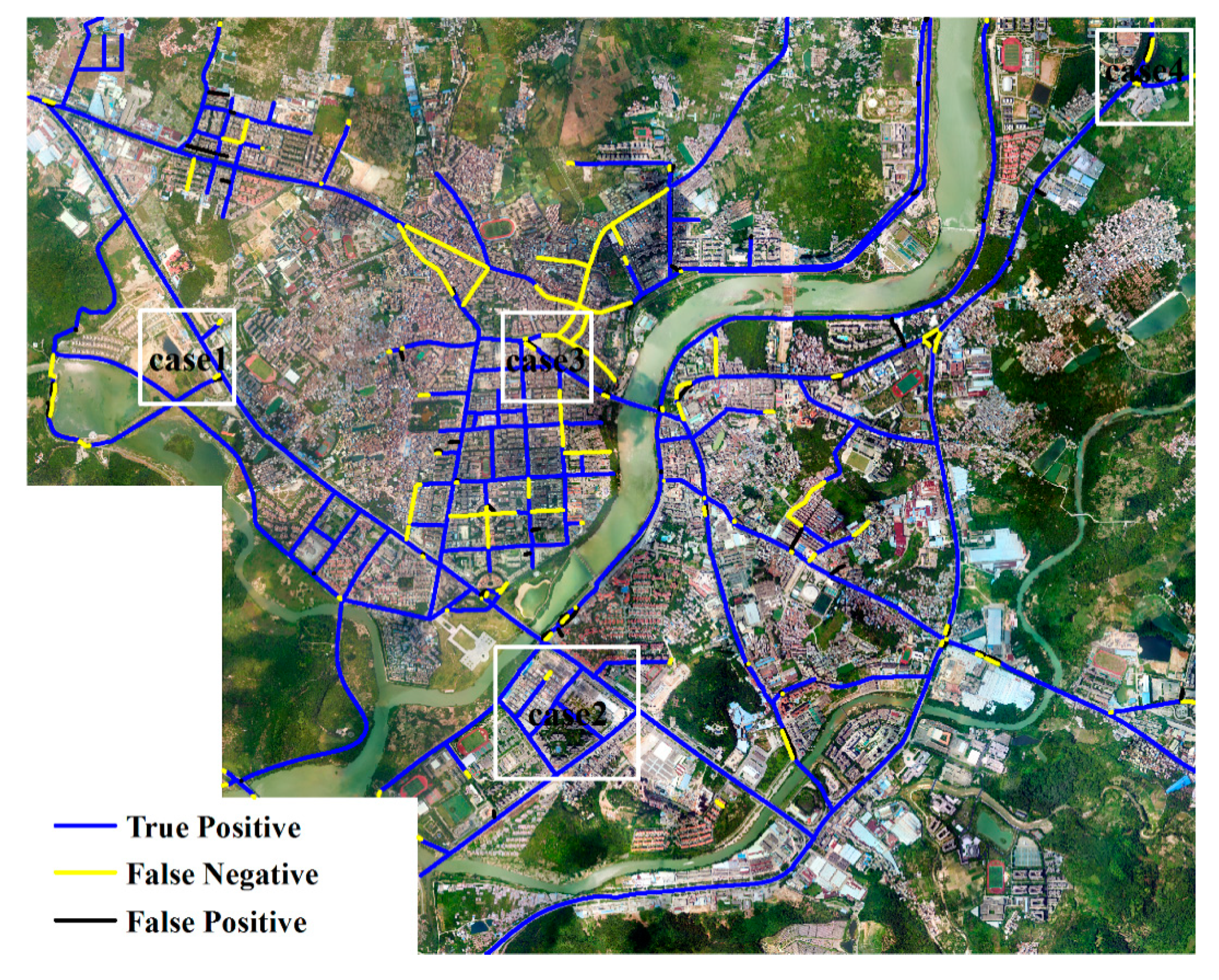
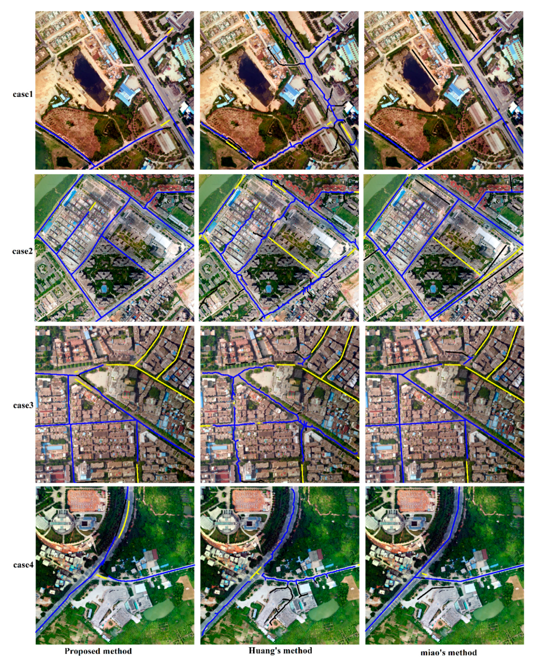
Figure 6 shows the road centerline network extraction for the Guangzhou dataset. Figure 7 shows the local comparison of road centerlines extracted by different methods. It is not difficult to find from Figure 6 that the proposed method can correctly extract most of the road centerlines for a wide range with complex scene, but there are some omissions. Case 1 in Figure 7 shows that in road segments where road widths change greatly, all three methods can extract the road centerlines. Nevertheless, comparison indicates that the road centerlines extracted by the proposed method are the most accurate, while one extracted by Huang’s method is less smooth, and some strip bares are identified as roads in one extracted by Miao’s method. Case 2 in Figure 7 shows the road centerline extraction of the area where there are many non-road impervious surface. In this scene, Huang’s method and Miao’s method are easy to mistake non-road impervious surface as the roads, and the narrow road segments are easy to be missed. Case 3 in Figure 7 shows the road centerline extraction of different methods in the case of serious interference. We can find from this case that it is difficult for all three methods to accurately extract the centerlines of the road segments in which most of area is shielded by shadows and trees. Case 4 in Figure 7 shows the road centerline extraction of the curved road segment and road intersections. According to the case, the road centerlines extracted by the proposed method are relatively smooth, but there is usually a deviation in the section of road segments with large curvature. However, Huang’s method can effectively overcome the deviation problem of road centerlines of curved road segments. Compared with the road centerlines extracted by proposed method, although the smoothness of one extracted by Miao’s method is low, the centerlines of road intersections are relatively accurate. Table 3 shows the quantitative assessment of road centerline extraction of different methods for the Guangzhou dataset. Compared with the New York dataset and the Vaihingen dataset, although the accuracies of the road centerline network slightly decreases, the completeness and correctness are both greater than 0.8, and even the correctness is as high as 0.9354. Meanwhile, the completeness, correctness, and quality of the road centerline network extracted by the proposed method are highest. Therefore, the proposed method can be applied to road centerline network extraction of a wide range with complex scenes.
5. Discussion
In this section, we take the New York dataset and the Vaihingen dataset as examples to discuss the effectiveness of key processes, parameter sensitivity, and computational cost of different methods.
5.1. Effectiveness Analysis of Key Processes
It can been seen from Figure 4 and Figure 5 that compared with Huang’s method and Miao’s method, the road centerline network extracted by the proposed method is more complete, and has fewer false road centerline segments. Moreover, Table 1 and Table 2 quantitatively show that the proposed method can achieve the highest completeness, correctness, and quality for both the New York dataset and the Vaihingen dataset. Therefore, the proposed method is an efficient solution for road centerline extraction from VHR aerial image and LiDAR data.
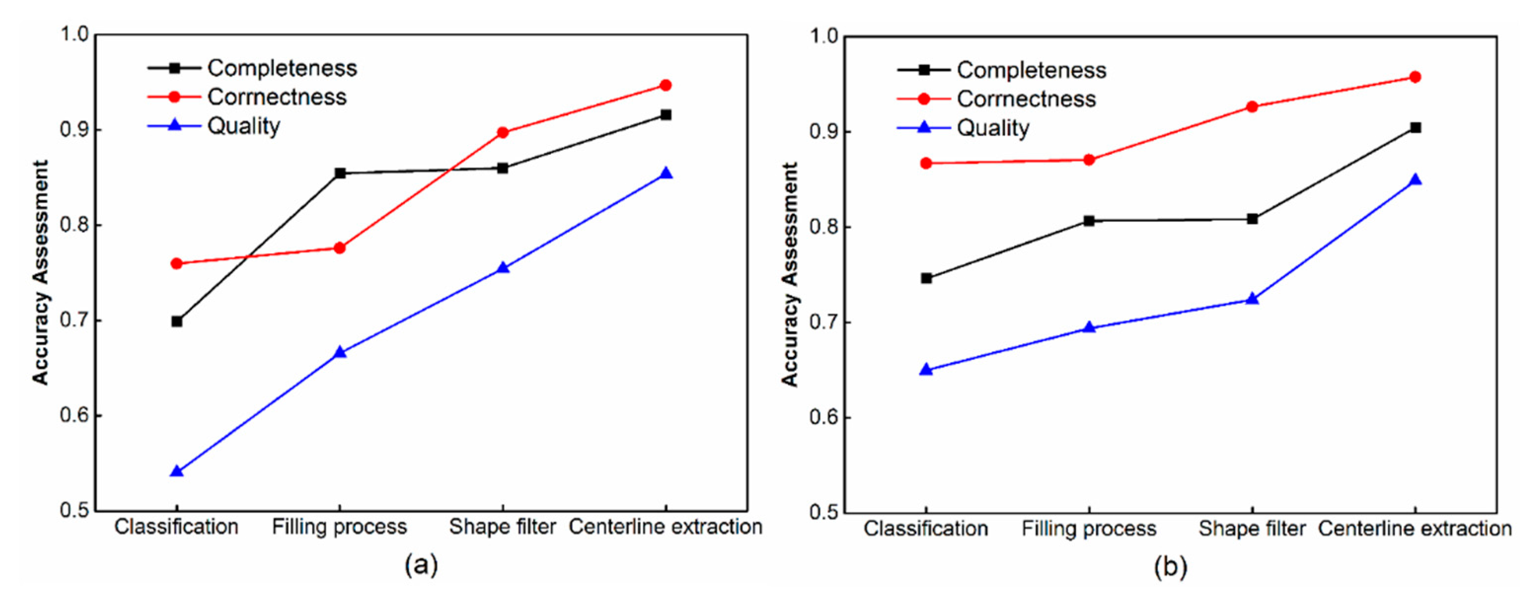
The proposed method is a multi-stage method. In order to analyze the effectiveness of each stage processing and the influence of them on road extraction, the accuracy assessment of the road centerline network obtained by each stage processing is carried out. Figure 8 shows the accuracy of road centerline network extracted by several key processing. Overall, all three key processing steps, namely, filling process, shape filter, and centerline extraction, can improve the completeness, correctness, and quality of road centerline extraction in the two datasets. However, the effects of different processing steps are not exactly same. The improvement of completeness is greater than that of correctness for the filling process, whereas the shape filter focuses on the improvement of correctness. The main reason is that the filling process only repairs the gaps caused by shadows and trees, but the false road segments are not processed, whereas the shape filter only removes a lot of false road segments. The centerline extraction has a great improvement on both completeness and correctness. This mainly because the road centerline fitting improves the position accuracy of road centerline network extraction.
5.2. Parameter Sensitivity Analysis
The scale parameter (T) determines the termination condition of object merging in the process of image segmentation, hence it is a key parameter for image segmentation. Many studies have analyzed the effect of T on the image segmentation. In this research, the influence of T on the road centerline network extraction is further analyzed.
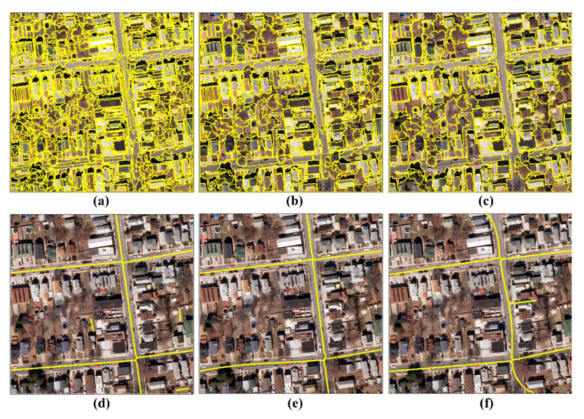
Figure 9 shows the image segmentation and road centerline extraction of different scale parameters using a small region in the New York dataset. It can be seen that the road centerline extraction of scale parameter 140 is superior to one of scale parameter 80 and 200. Some bare lands are misclassified as roads in the road centerline extraction of scale parameter 80, whereas the accuracy of the road centerline extraction of scale parameter 200 is relatively low, and there are some false road centerline segments adjacent to the road centerline network. The main reason is that the road is over-segmented and some bare lands present elongated structure similar to road segments when the scale parameter is set to 80, while the road is under-segmentation and other impervious surfaces adjacent to the road are merged into road objects when the scale parameter is set to 200.
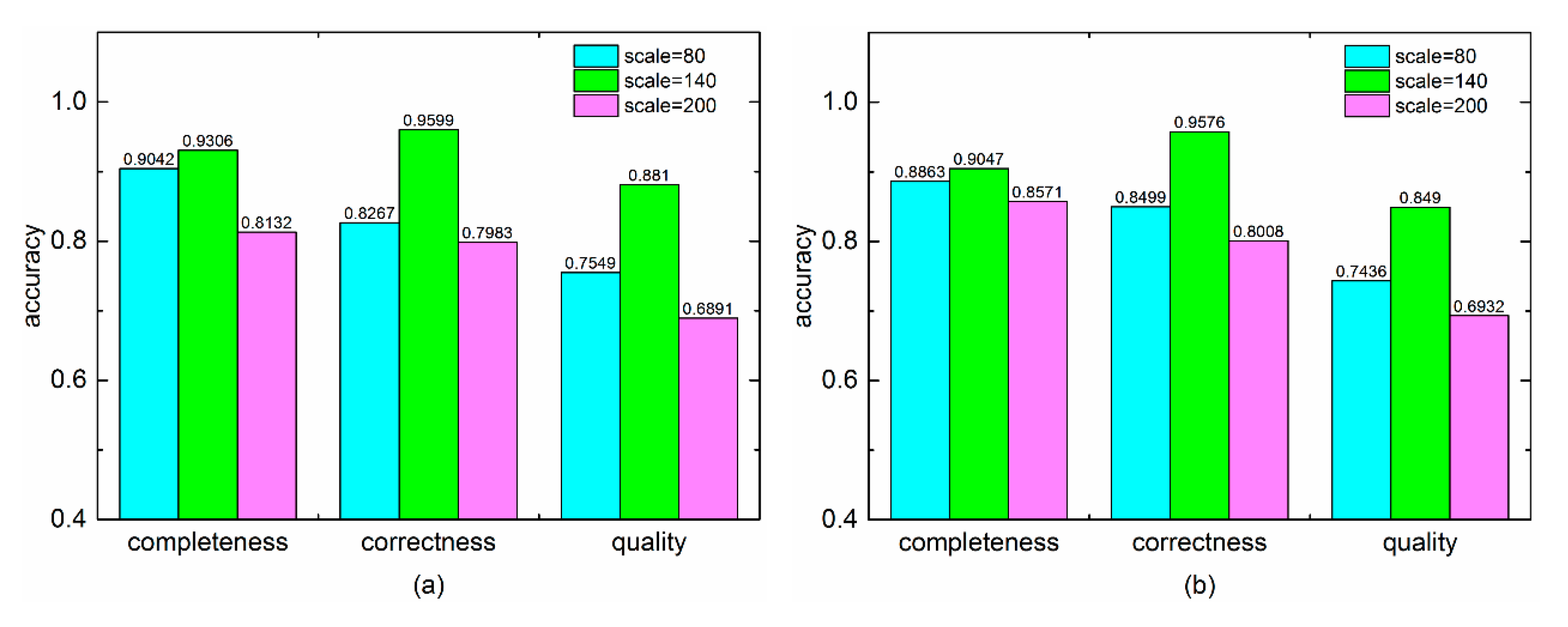
Figure 10 shows the accuracies of road centerline network extracted by different scale parameters. The investigations for both two datasets show a similar conclusion—that the road centerline extraction of scale parameter 140 has the highest completeness, correctness, and quality. Compared with over-segmentation, a slight under-segmentation can achieve better road centerline extraction for the proposed method.
5.3. Computational Cost Analysis
In this study, all the experiments are performed on a PC with a Intel Core 4 CPU at 3.20 GHz and 24-GB RAM. Image segmentation is performed by eCognition software, and other experimental processing run under MATLAB R2014a. As Huang’s method and proposed method are implemented on two different platforms, the computational cost is counted independently. Each experiment is repeated five times, and the average running time is taken as the computational cost. Table 4 shows the computational costs of different methods for the New York and Vaihingen datasets. Although the computational cost of the proposed method is slightly greater than that of Huang’s method and Miao’s method, the accuracy of the proposed method is higher than that of the two comparison methods. What’s more, the computational cost of the proposed method is far less than that of manual drawing. Thus, in terms of computational cost, the proposed method is still an effective solution for road centerline extraction in complex scene.
6. Conclusions
This study develops a method to extract road centerline network in complex scenes using both aerial VHR images and LiDAR data. A MABR-based interference filling approach is developed to remove the negative influences of shadows, trees, and cars on road centerline extraction. A multistep approach that integrates the morphology thinning, Harris corner detection, and least square fitting is proposed to accurately extract the road centerline from the complex road networks.
Three datasets are chosen to assess the effectiveness and adaptability of the proposed method by comparison with two existing methods. The results based on the three datasets show that the proposed method can obtain the highest completeness, correctness, and quality. For straight road sections, the proposed method can effectively eliminate the negative influences of shadows and trees, and obtain accurate road centerlines. However, for curved road segments that are severely obstructed by shadows and trees, the effect of the proposed method needs to be further improved. In general, although the proposed method has a little limitation, it can effectively reduce the workload of road mapping, and thus it is still an effective solution for road centerline extraction in a complex scene.
In future work, the performance of the proposed method for curved road segments severely obstructed by shadows and trees will be further improved. What is more, road change detection combined with the road vector map will be carried out to expand the application of the proposed method.
Author Contributions
Z.Z. and X.Z. conceived and designed the method; Z.Z. performed the experiments and wrote the manuscript; Y.S. and P.Z. revised the manuscript.
Funding
This research was funded by the National Natural Science Foundation of China (Grant No. 41431178), the Natural Science Foundation of Guangdong Province in China (Grant No. 2016A030311016), and the National Administration of Surveying, Mapping and Geoinformation of China (Grant No. GZIT2016-A5-147).
Acknowledgments
The authors would like to thank the anonymous reviewers for their constructive comments. The authors are also grateful to Kyle Bradbury et al. for providing the New York dataset and the German Society for Photogrammetry, Remote Sensing, and Geoinformation for providing the Vaihingen dataset.
Conflicts of Interest
The authors declare no conflict of interest.
Abbreviations
The following abbreviations are used in this manuscript:
| VHR | Very-High-Resolution |
| LiDAR | Light Detection and Ranging |
| MABR | minimum area bounding rectangle |
| MBR | minimum bounding rectangle |
| FNEA | fractal net evolution approach |
| DSM | digital surface model |
| nDSM | normalized digital surface model |
| DTM | digital terrain model |
| OSM | open Street Map |
| SOLI | skeleton-based object linearity index |
| MHL | morphology thinning, Harris corner detection, and least square fitting |
References
- Das, S.; Mirnalinee, T.; Varghese, K. Use of salient features for the design of a multistage framework to extract roads from high-resolution multispectral satellite images. IEEE Trans. Geosci. Remote Sens. 2011, 49, 3906–3931. [Google Scholar] [CrossRef]
- Wang, J.; Qin, Q.; Gao, Z.; Zhao, J.; Ye, X. A new approach to urban road extraction using high-resolution aerial image. ISPRS Int. J. Geo-Inf. 2016, 5, 114. [Google Scholar] [CrossRef]
- Maboudi, M.; Amini, J.; Hahn, M.; Saati, M. Road network extraction from vhr satellite images using context aware object feature integration and tensor voting. Remote Sens. 2016, 8, 637. [Google Scholar] [CrossRef]
- Gao, L.; Shi, W.; Miao, Z.; Lv, Z. Method based on edge constraint and fast marching for road centerline extraction from very high-resolution remote sensing images. Remote Sens. 2018, 10, 900. [Google Scholar] [CrossRef]
- Miao, Z.; Shi, W.; Gamba, P.; Li, Z. An object-based method for road network extraction in vhr satellite images. IEEE J. Sel. Top. Appl. Earth Obs. Remote Sens. 2015, 8, 4853–4862. [Google Scholar] [CrossRef]
- Mena, J.B. State of the art on automatic road extraction for gis update: A novel classification. Pattern Recognit. Lett. 2003, 24, 3037–3058. [Google Scholar] [CrossRef]
- Miao, Z.; Wang, B.; Shi, W.; Zhang, H. A semi-automatic method for road centerline extraction from vhr images. IEEE Geosci. Remote Sens. Lett. 2014, 11, 1856–1860. [Google Scholar] [CrossRef]
- Cardim, G.; Silva, E.; Dias, M.; Bravo, I.; Gardel, A. Statistical evaluation and analysis of road extraction methodologies using a unique dataset from remote sensing. Remote Sens. 2018, 10, 620. [Google Scholar] [CrossRef]
- Benjamin, S.; Gaydos, L. Spatial resolution requirements for automated cartographic road extraction. Photogramm. Eng. Remote Sens. 1990, 56, 93–100. [Google Scholar]
- Liu, J.; Qin, Q.; Li, J.; Li, Y. Rural road extraction from high-resolution remote sensing images based on geometric feature inference. ISPRS Int. J. Geo-Inf. 2017, 6, 314. [Google Scholar] [CrossRef]
- Hu, J.; Razdan, A.; Femiani, J.C.; Cui, M.; Wonka, P. Road network extraction and intersection detection from aerial images by tracking road footprints. IEEE Trans. Geosci. Remote Sens. 2007, 45, 4144–4157. [Google Scholar] [CrossRef]
- Shi, W.; Zhu, C. The line segment match method for extracting road network from high-resolution satellite images. IEEE Trans. Geosci. Remote Sens. 2002, 40, 511–514. [Google Scholar]
- Song, M.; Civco, D. Road extraction using svm and image segmentation. Photogramm. Eng. Remote Sens. 2004, 70, 1365–1371. [Google Scholar] [CrossRef]
- Mokhtarzade, M.; Zoej, M.V. Road detection from high-resolution satellite images using artificial neural networks. Int. J. Appl. Earth Obs. Geoinf. 2007, 9, 32–40. [Google Scholar] [CrossRef] [Green Version]
- Huang, X.; Zhang, L. Road centreline extraction from high-resolution imagery based on multiscale structural features and support vector machines. Int. J. Remote Sens. 2009, 30, 1977–1987. [Google Scholar] [CrossRef]
- Sujatha, C.; Selvathi, D. Connected component-based technique for automatic extraction of road centerline in high resolution satellite images. EURASIP J. Image Video Process. 2015, 2015, 8. [Google Scholar] [CrossRef]
- Shi, W.; Miao, Z.; Wang, Q.; Zhang, H. Spectral–spatial classification and shape features for urban road centerline extraction. IEEE Geosci. Remote Sens. Lett. 2014, 11, 788–792. [Google Scholar]
- Zhao, J.; You, S.; Huang, J. In Rapid extraction and updating of road network from airborne lidar data. In Proceedings of the Applied Imagery Pattern Recognition Workshop (AIPR), Washington, DC, USA, 11–13 October 2011; pp. 1–7. [Google Scholar]
- Choi, Y.-W.; Jang, Y.-W.; Lee, H.-J.; Cho, G.-S. Three-dimensional lidar data classifying to extract road point in urban area. IEEE Geosci. Remote Sens. Lett. 2008, 5, 725–729. [Google Scholar] [CrossRef]
- Xu, J.-Z.; Wan, Y.-C.; Lai, Z.-L. Multi-scale method for extracting road centerlines from lidar datasets. Infrared Laser Eng. 2009, 6, 034. [Google Scholar]
- Hu, X.; Li, Y.; Shan, J.; Zhang, J.; Zhang, Y. Road centerline extraction in complex urban scenes from lidar data based on multiple features. IEEE Trans. Geosci. Remote Sens. 2014, 52, 7448–7456. [Google Scholar]
- Hui, Z.; Hu, Y.; Jin, S.; Yevenyo, Y.Z. Road centerline extraction from airborne lidar point cloud based on hierarchical fusion and optimization. ISPRS J. Photogramm. Remote Sens. 2016, 118, 22–36. [Google Scholar] [CrossRef]
- Meng, X.; Wang, L.; Currit, N. Morphology-based building detection from airborne lidar data. Photogramm. Eng. Remote Sens. 2009, 75, 437–442. [Google Scholar] [CrossRef]
- Hu, X.; Ye, L.; Pang, S.; Shan, J. Semi-global filtering of airborne lidar data for fast extraction of digital terrain models. Remote Sens. 2015, 7, 10996–11015. [Google Scholar] [CrossRef]
- Clode, S.; Kootsookos, P.J.; Rottensteiner, F. The automatic extraction of roads from lidar data. In Proceedings of the International Society for Photogrammetry and Remote Sensing′s Twentieth Annual Congress, Istanbul, Turkey, 12–23 July 2004; pp. 231–236. [Google Scholar]
- Gargoum, S.; El-Basyouny, K. Automated extraction of road features using LiDARdata: A review of LiDAR applications in transportation. In Proceedings of the 4th International Conference on Transportation Information and Safety, Banff, AB, Canada, 8–10 August 2017; pp. 563–574. [Google Scholar]
- Liu, L.; Lim, S. A framework of road extraction from airborne lidar data and aerial imagery. J. Spatial Sci. 2016, 61, 263–281. [Google Scholar] [CrossRef]
- Sameen, M.I.; Pradhan, B. A two-stage optimization strategy for fuzzy object-based analysis using airborne lidar and high-resolution orthophotos for urban road extraction. J. Sens. 2017. [Google Scholar] [CrossRef]
- Hu, X.; Tao, C.V.; Hu, Y. Automatic Road Extraction from Dense Urban Area by Integrated Processing of High Resolution Imagery and Lidar Data; International Archives of Photogrammetry, Remote Sensing and Spatial Information Sciences: Istanbul, Turkey, 2004; Volume 35, p. B3. [Google Scholar]
- Grote, A.; Heipke, C.; Rottensteiner, F. Road network extraction in suburban areas. Photogramm. Rec. 2012, 27, 8–28. [Google Scholar] [CrossRef]
- Hu, X.; Zhang, Z.; Tao, C.V. A robust method for semi-automatic extraction of road centerlines using a piecewise parabolic model and least square template matching. Photogramm. Eng. Remote Sens. 2004, 70, 1393–1398. [Google Scholar] [CrossRef]
- Miao, Z.; Shi, W.; Samat, A.; Lisini, G.; Gamba, P. Information fusion for urban road extraction from vhr optical satellite images. IEEE J. Sel. Top. Appl. Earth Obs. Remote Sens. 2016, 9, 1817–1829. [Google Scholar] [CrossRef]
- Shi, W.; Miao, Z.; Debayle, J. An integrated method for urban main-road centerline extraction from optical remotely sensed imagery. IEEE Trans. Geosci. Remote Sens. 2014, 52, 3359–3372. [Google Scholar] [CrossRef]
- Jang, B.-K.; Chin, R.T. Analysis of thinning algorithms using mathematical morphology. IEEE Trans. Pattern Anal. Mach. Intell. 1990, 12, 541–551. [Google Scholar] [CrossRef]
- Zhang, Q.; Couloigner, I. Accurate centerline detection and line width estimation of thick lines using the radon transform. IEEE Trans. Image Process. 2007, 16, 310–316. [Google Scholar] [CrossRef] [PubMed]
- Poullis, C.; You, S. Delineation and geometric modeling of road networks. ISPRS J. Photogramm. Remote Sens. 2010, 65, 165–181. [Google Scholar] [CrossRef]
- Kyle, B.; Benjamin, B.; Leslie, C.; Timothy, J.; Sebastian, L.; Richard, N.; Sophia, P.; Sunith, S.; Hoel, W.; Yue, X. Arlington, Massachusetts—Aerial imagery object identification dataset for building and road detection, and building height estimation. Figshare Filset 2016. [Google Scholar] [CrossRef]
- Rottensteiner, F.; Sohn, G.; Gerke, M.; Wegner, J.D. ISPRS Test Project on Urban Classification and 3d Building Reconstruction. Commission III-Photogrammetric Computer Vision and Image Analysis, Working Group III/4-3D Scene Analysis. 2013, pp. 1–17. Available online: http://www2.isprs.org/commissions/comms/wg4/detection-and-reconstruction.html (accessed on 7 January 2013).
- Meng, X.; Wang, L.; Silván-Cárdenas, J.L.; Currit, N. A multi-directional ground filtering algorithm for airborne lidar. ISPRS J. Photogramm. Remote Sens. 2009, 64, 117–124. [Google Scholar] [CrossRef]
- Haklay, M.; Weber, P. Openstreetmap: User-generated street maps. IEEE Pervasive Comput. 2008, 7, 12–18. [Google Scholar] [CrossRef]
- Hay, G.J.; Blaschke, T.; Marceau, D.J.; Bouchard, A. A comparison of three image-object methods for the multiscale analysis of landscape structure. ISPRS J. Photogramm. Remote Sens. 2003, 57, 327–345. [Google Scholar] [CrossRef]
- Breiman, L. Random forests. Mach. Learn. 2001, 45, 5–32. [Google Scholar] [CrossRef]
- Ning, X.; Lin, X. An index based on joint density of corners and line segments for built-up area detection from high resolution satellite imagery. ISPRS Int. J. Geo-Inf. 2017, 6, 338. [Google Scholar] [CrossRef]
- Guo, Z.; Du, S. Mining parameter information for building extraction and change detection with very high-resolution imagery and GIS data. Geosci. Remote Sens. 2017, 54, 38–63. [Google Scholar] [CrossRef]
- Tian, S.; Zhang, X.; Tian, J.; Sun, Q. Random forest classification of wetland landcovers from multi-sensor data in the arid region of Xinjiang, China. Remote Sens. 2016, 8, 954. [Google Scholar] [CrossRef]
- Rodriguez-Galiano, V.F.; Ghimire, B.; Rogan, J.; Chica-Olmo, M.; Rigol-Sanchez, J.P. An assessment of the effectiveness of a random forest classifier for land-cover classification. ISPRS J. Photogramm. Remote Sens. 2012, 67, 93–104. [Google Scholar] [CrossRef]
- Blaschke, T. Object based image analysis for remote sensing. ISPRS J. Photogramm. Remote Sens. 2010, 65, 2–16. [Google Scholar] [CrossRef]
- Li, X.; Shao, G. Object-based land-cover mapping with high resolution aerial photography at a county scale in midwestern USA. Remote Sens. 2014, 6, 11372–11390. [Google Scholar] [CrossRef]
- Gu, H.; Han, Y.; Yang, Y.; Li, H.; Liu, Z.; Soergel, U.; Blaschke, T.; Cui, S. An efficient parallel multi-scale segmentation method for remote sensing imagery. Remote Sens. 2018, 10, 590. [Google Scholar] [CrossRef]
- Witharana, C.; Lynch, H.J. An object-based image analysis approach for detecting penguin guano in very high spatial resolution satellite images. Remote Sens. 2016, 8, 375. [Google Scholar] [CrossRef]
- Feng, Q.; Liu, J.; Gong, J. Uav remote sensing for urban vegetation mapping using random forest and texture analysis. Remote Sens. 2015, 7, 1074–1094. [Google Scholar] [CrossRef]
- Hinz, S.; Baumgartner, A. Automatic extraction of urban road networks from multi-view aerial imagery. ISPRS J. Photogramm. Remote Sens. 2003, 58, 83–98. [Google Scholar] [CrossRef] [Green Version]
- Huang, X.; Zhang, L. An adaptive mean-shift analysis approach for object extraction and classification from urban hyperspectral imagery. IEEE Trans. Geosci. Remote Sens. 2008, 46, 4173–4185. [Google Scholar] [CrossRef]
- Kwak, E.; Habib, A. Automatic representation and reconstruction of dbm from lidar data using recursive minimum bounding rectangle. ISPRS J. Photogramm. Remote Sens. 2014, 93, 171–191. [Google Scholar] [CrossRef]
- Misra, I.; Moorthi, S.M.; Dhar, D.; Ramakrishnan, R. An automatic satellite image registration technique based on harris corner detection and random sample consensus (RANSAC) outlier rejection model. In Proceedings of the 1st International Conference on Recent Advances in Information Technology (RAIT), Dhanbad, India, 15–17 March 2012; pp. 68–73. [Google Scholar]
- Heipke, C.; Mayer, H.; Wiedemann, C.; Jamet, O. Evaluation of automatic road extraction. Int. Arch. Photogramm. Remote Sens. 1997, 32, 151–160. [Google Scholar]
Figure 1.
The experimental materials for three datasets. The first, second, and third rows represent the New York dataset, the Vaihingen dataset, and the Guangzhou dataset, respectively.
Figure 1.
The experimental materials for three datasets. The first, second, and third rows represent the New York dataset, the Vaihingen dataset, and the Guangzhou dataset, respectively.

Figure 2.
The workflow of the proposed method for extracting the road centerline network. VHR—very-high-resolution; LiDAR—light detection and ranging; OSM—OpenStreetMap.
Figure 2.
The workflow of the proposed method for extracting the road centerline network. VHR—very-high-resolution; LiDAR—light detection and ranging; OSM—OpenStreetMap.

Figure 3.
Results of road network extraction of a test area in the New York dataset are shown for (a) image segmentation; (b) random forest classification; (c) the road network processed by the filling approach; and (d) the road network obtained by shape filtering.
Figure 3.
Results of road network extraction of a test area in the New York dataset are shown for (a) image segmentation; (b) random forest classification; (c) the road network processed by the filling approach; and (d) the road network obtained by shape filtering.

Figure 4.
The road centerline network extraction of different methods for New York dataset, in which (a–c) are shown as the road centerline network extraction of the proposed method, Huang’s method [15] and Miao’s method [32], respectively; (d–f) show the corresponding road centerline extraction marked with red rectangle and the road is superimposed on the false-color composite image.

Figure 5.
The road centerline network extraction for Vaihingen dataset. (a) The initial road network extracted by object-based classification; (b) the road network obtained by shape filter; (c) the road centerline network extracted by morphology thinning; (d–f) are shown the road centerline network of the proposed method, Huang’s method [13] and Miao’s method [30], respectively.

Figure 6.
The road centerline network extracted by the proposed method and original image superposition. True positives are shown in blue, false positives in yellow, and false negatives in black.
Figure 6.
The road centerline network extracted by the proposed method and original image superposition. True positives are shown in blue, false positives in yellow, and false negatives in black.

Figure 7.
Comparison of the road centerline network extraction of different methods for the Guangzhou dataset. True positives are shown in blue, false positives in yellow, and false negatives in black.
Figure 7.
Comparison of the road centerline network extraction of different methods for the Guangzhou dataset. True positives are shown in blue, false positives in yellow, and false negatives in black.

Figure 8.
The accuracies of key processing result including classification, filling process, shape filter, and centerline extraction. (a) New York dataset; (b) Vaihingen dataset.
Figure 8.
The accuracies of key processing result including classification, filling process, shape filter, and centerline extraction. (a) New York dataset; (b) Vaihingen dataset.

Figure 9.
The road centerline extraction of different scale parameter. (a–c) show the image segmentation of the scale parameter as 80, 140, and 200, respectively; (d–f) show the road centerline extraction of corresponding scale parameter.
Figure 9.
The road centerline extraction of different scale parameter. (a–c) show the image segmentation of the scale parameter as 80, 140, and 200, respectively; (d–f) show the road centerline extraction of corresponding scale parameter.

Figure 10.
Accuracies of road centerline network extraction of different segmentation scales. (a,b) are shown for the New York and Vaihingen datasets, respectively.
Figure 10.
Accuracies of road centerline network extraction of different segmentation scales. (a,b) are shown for the New York and Vaihingen datasets, respectively.


Table 1.
Quantitative assessment of road centerline extraction of different methods for the New York dataset.
Table 1.
Quantitative assessment of road centerline extraction of different methods for the New York dataset.
| Method | Completeness | Correctness | Quality |
|---|---|---|---|
| Proposed method | 0.9306 | 0.9599 | 0.8810 |
| Huang’s method | 0.7939 | 0.9313 | 0.7162 |
| Miao’s method | 0.8653 | 0.8785 | 0.7737 |
Table 2.
Quantitative assessment of road centerline extraction of different methods for the Vaihingen dataset.
Table 2.
Quantitative assessment of road centerline extraction of different methods for the Vaihingen dataset.
| Method | Completeness | Correctness | Quality |
|---|---|---|---|
| Proposed method | 0.9047 | 0.9576 | 0.8490 |
| Huang’s method | 0.8139 | 0.8829 | 0.7007 |
| Miao’s method | 0.8817 | 0.8821 | 0.7870 |
Table 3.
Quantitative assessment of road centerline extraction of different methods for the Guangzhou dataset.
Table 3.
Quantitative assessment of road centerline extraction of different methods for the Guangzhou dataset.
| Method | Completeness | Correctness | Quality |
|---|---|---|---|
| Proposed method | 0.8019 | 0.9354 | 0.7522 |
| Huang’s method | 0.7314 | 0.8211 | 0.6890 |
| Miao’s method | 0.7832 | 0.8726 | 0.7169 |
Table 4.
Computational costs of different methods for the New York and Vaihingen datasets.
| New York Dataset | Vaihingen Dataset | |||||
|---|---|---|---|---|---|---|
| Proposed Method | Huang’s Method | Miao’s Method | Proposed Method | Huang’s Method | Miao’s Method | |
| Image segmentation | 687 s | 846 s | --- | 529 s | 581 s | --- |
| Other processing | 1585 s | 723 s | 2143 s | 1137 s | 507 s | 1479 s |
| Total | 2272 s | 1569 s | 2143 s | 1666 s | 1088 s | 1479 s |
© 2018 by the authors. Licensee MDPI, Basel, Switzerland. This article is an open access article distributed under the terms and conditions of the Creative Commons Attribution (CC BY) license (http://creativecommons.org/licenses/by/4.0/).
Share and Cite
MDPI and ACS Style
Zhang, Z.; Zhang, X.; Sun, Y.; Zhang, P. Road Centerline Extraction from Very-High-Resolution Aerial Image and LiDAR Data Based on Road Connectivity. Remote Sens. 2018, 10, 1284. https://doi.org/10.3390/rs10081284
AMA Style
Zhang Z, Zhang X, Sun Y, Zhang P. Road Centerline Extraction from Very-High-Resolution Aerial Image and LiDAR Data Based on Road Connectivity. Remote Sensing. 2018; 10(8):1284. https://doi.org/10.3390/rs10081284
Chicago/Turabian StyleZhang, Zhiqiang, Xinchang Zhang, Ying Sun, and Pengcheng Zhang. 2018. "Road Centerline Extraction from Very-High-Resolution Aerial Image and LiDAR Data Based on Road Connectivity" Remote Sensing 10, no. 8: 1284. https://doi.org/10.3390/rs10081284
Note that from the first issue of 2016, this journal uses article numbers instead of page numbers. See further details here.