Land Cover Change Detection Using Multiple Shape Parameters of Spectral and NDVI Curves


1
College of Geo-Exploration Science and Technology, Jilin University, Changchun 130026, China
2
National Geomatics Center of China, Beijing 100830, China
3
School of Geography Faculty of Geographical Science, Beijing Normal University, Beijing 100875, China
4
School of Environmental Science and Engineering, Suzhou University of Science and Technology, Suzhou 215011, China
*
Authors to whom correspondence should be addressed.
Remote Sens. 2018, 10(8), 1251; https://doi.org/10.3390/rs10081251
Submission received: 12 July 2018
/
Revised: 3 August 2018
/
Accepted: 4 August 2018
/
Published: 9 August 2018
(This article belongs to the Section Remote Sensing Image Processing)
Abstract
:Spectral and NDVI values have been used to calculate the change magnitudes of land cover, but may result in many pseudo-changes because of inter-class variance. Recently, the shape information of spectral or NDVI curves such as direction, angle, gradient, or other mathematical indicators have been used to improve the accuracy of land cover change detection. However, these measurements, in terms of the single shape features, can hardly capture the complete trends of curves affected by the unsynchronized phenology. Therefore, the calculated change magnitudes are indistinct such that changes and no-changes have a low contrast. This problem has prevented traditional change detection methods from achieving a higher accuracy using bi-temporal images or NDVI time series. In this paper, a multiple shape parameters-based change detection method is proposed by combining the spectral correlation operator and the shape features of NDVI temporal curves (phase angle cumulant, baseline cumulant, relative cumulation rate, and zero-crossing rate). The change magnitude is derived by integrating all the inter-annual differences of these shape parameters. The change regions are discriminated by an automated threshold selection method known as histogram concavity analysis. The results showed that the mean differences in the change magnitudes of the proposed method between 2100 changed and 2523 unchanged pixels was 32%, the overall accuracy was approximately 88%, and the kappa coefficient was 0.76. A comparative analysis was conducted with bi-temporal image-based methods and NDVI time series-based methods, and we demonstrate that the proposed method is more effective and robust than traditional methods in achieving high-contrast change magnitudes and accuracy.
1. Introduction
Land cover dynamics and their spatiotemporal information play a vital role in many scientific fields, such as natural resources management, environmental research, climate modeling, and earth biogeochemistry studies [1,2,3]. In the past decades, a variety of bi-temporal change detection methods have been developed to monitor land cover conversions between two years based onLandsat images or NDVI time series [4,5,6,7]. However, the method of comparing the responses of a single image band or NDVI which is directly accepted by some previous algorithms (e.g., image differencing and image ratioing) may lead to pseudo-changes, which hampers the monitoring process from local to regional scales [8,9,10]. Individual values in the spectrum or temporal curve of land cover type are more vulnerable to environmental factors and thus result in data uncertainty [11,12]. If change magnitudes were calculated based on contaminated values of the spectrum or temporal curves, pseudo-changes would be generated. In contrast, all values of the spectrum or NDVI temporal curves are more robust than single values. Therefore, it is valuable to explore the potentiality of the shape of spectra and the NDVI temporal curve for obtaining more accurate change detection results.
In order to utilize the shape information of the spectrum, researchers began to consider the overall difference of the spectrum from different perspectives. For example, the change vector analysis (CVA) method compares the difference of spectral vectors which consist of many values [13]. In two-dimensional space, the magnitude and direction of curves are adopted to measure the spectral shape. It is useful to find the changed pixels using all of the image bands and provide “from–to”-type change information [14,15]. However, the demand for reliable radiometric image correction is strict in some cases, limiting its application. Nevertheless, it is significant in that the method provides a way to compare the whole difference of spectral shapes. After that, the algorithm known as spectral angle mapper (SAM) was developed to determine the spectral similarity between each pair of spectra treated as a vector [16]. In this technique, the angles of two curves in multi-dimensional space are taken as a type of shape information to measure the difference of the spectra [17]. Although these algorithms consider the shape information of the spectral curves, some pseudo-changes induced by inter-class spectral variation cannot be avoided. Therefore, a spectral gradient-based change detection approach (SGD) was recently developed, aiming to address this difficulty [18]. It uses the spectral gradient to quantitatively describe the shape of the spectrum of a given land cover type, and operates on the belief that gradient differences can compress the pseudo-changes more effectively than previous methods. The transformation from spectral space to the spectral gradient space of SGD helps to counteract the adverse effects caused by interference factors, and eliminates the pseudo-changes. However, pseudo-changes could no longer be eliminated when phenological factors altered most spectral values and changed the spectral shape of land cover types.
NDVI time series are rich in phenological dynamics information, which could help to reduce pseudo-changes caused by spectral variance [19,20,21,22]. The temporal curves of NDVI have been used to detect typical land cover changes, such as grassland degradation, deforestation, wetland vegetation, and crop rotation [23,24,25,26]. In an automated land cover updating approach, the NDVI temporal curve in two-dimensional space was taken in its entirety to remove pseudo-changes from bi-temporal Landsat data [27]. Then, the gradient was adopted to describe the shape information of the NDVI temporal curve in the NDVI gradient difference (NDVI-GD) method [28]. This method detects change areas by considering the NDVI temporal curve shape and value differences simultaneously. These approaches effectively reduce the influence of phenological differences between images from two different dates. Unfortunately, the shape features of NDVI temporal curves have not been exploited enough. The change magnitudes of these approaches are derived from the accumulation of all differences between two values in a single time point. Their computing principle needs the compared values in two NDVI temporal curves to change with the same step in different years. It is almost impossible for natural phenological dynamics to be affected by solar illumination, air temperature, soil moisture, and other factors [29]. Otherwise, differences in some time points that are more likely to be changed could be offset by the differences in other time points that are more likely to be unchanged. As a result, the change magnitude might be confused by these conflicting differences that imply that the real changes are not strong enough and pseudo-changes are not weak enough.
Even if the shape features of a spectrum or an NDVI temporal curve such as angle, direction, and gradient have been utilized, some pseudo-changes cannot be reduced due to phenological difference. One of the possible reasons is that the shape of the NDVI temporal curve is more complicated than the spectrum, considering that the fluctuations are affected by various factors. Comparing the NDVI temporal curves directly from value to value cannot avoid the adverse effects from unsynchronized fluctuations. Therefore, it is preferable to use the overall shape features of the NDVI temporal curve in order to avoid this problem. Since the NDVI temporal curve reflects the phenological change of land cover, its shape features can be described with a reference to seasonal parameters. For instance, some of the parameters are the beginning of the season, the end of the season, amplitude, and the rate of increase [19]. The phenological variability of land cover could be measured by these metrics [29]. Therefore, using these parameters or metrics to model the shape feature of the NDVI temporal curve is feasible. Considering the different spectrum of the same land cover type, the correlation operator of the spectrum is more appropriate to ensure that the shape information of the spectrum is utilized but not overexploited. The integration of advantages from the spectra and NDVI temporal curve could further reduce the pseudo-changes and allow easier discrimination of real changes from non-changes.
In this study, a multiple shape parameters-based change detection method using one pair of Landsat images from two years and two yearly NDVI time series was developed to calculate the change magnitude with high contrast under the confusions of conflicting differences and improve change detection accuracy. For the NDVI temporal curve, shape parameters were mainly formed by reconstructions of seasonal parameters and the application of zero-crossing rate. The spectral correlation operator was adopted as a special spectral shape parameter. The change magnitudes were derived from differences of all shape parameters and integrated as one final change magnitude. Then, change discrimination was applied based on an auto-threshold method. It mainly consisted of three parts, which were change magnitude calculation, change magnitude integration, and change region discrimination, as described in Section 2. Section 3 presents the experimental results and reports on the accuracy of the proposed method with a comparison regarding the several bi-temporal images or NDVI time series-based methods mentioned above. The discussion and conclusions are provided in Section 4 and Section 5, respectively.
2. Methodology
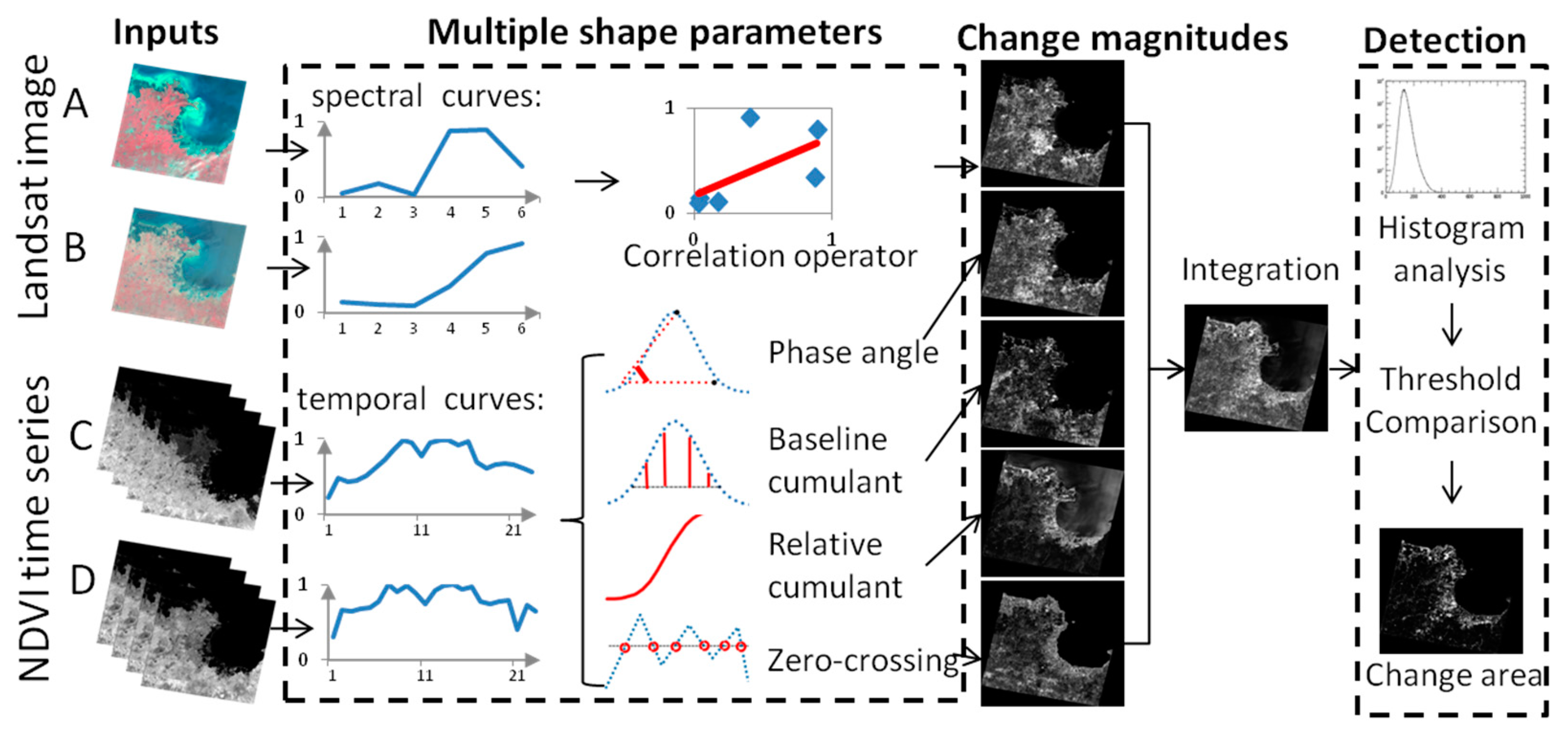
The main idea of the multiple shape parameter-based (MSP) change detection method is the utilization of shape features from both the spectrum and the NDVI temporal curve to calculate a high-contrast change magnitude that can mostly discriminate the change region from various change magnitude types. It includes three major components: change magnitude calculation (see Section 2.1), change magnitude integration (see Section 2.2), and change region determination (see Section 2.3). Figure 1 gives the framework of the MSP method. In the change magnitude calculation part, five shape parameters (correlation operator for spectral curves, phase angle, baseline cumulant, relative cumulant, and zero-crossing rate for NDVI temporal curves) are adopted to describe the shape features of the spectrum and the NDVI temporal curve and perform measurements from these different parameters. The differences of bi-temporal multispectral image pairs or NDVI time-series pairs are taken to calculate the change magnitudes independently using these shape parameters. In the change magnitude integration part, the units of different change magnitudes are assimilated by standard normalization. These unified change magnitudes are integrated with a weighting function. Finally, the changed and unchanged regions are acquired by comparing the change magnitude with a threshold.
2.1. Change Magnitudes From the Spectrum and the NDVI Curve
2.1.1. Shape Parameters of NDVI Temporal Curve
Inter-annual trends in the NDVI time series derived from remote sensing data can be used to distinguish between natural land cover variability and land cover change [20]. Phenological land cover information remains in the shape features (e.g., amplitude and fluctuation) of the NDVI temporal curve at the inter-annual time scale. Throughout the year, seasonal phenologies affect these features during certain periods. Therefore, these features can be united to describe the annual characteristic of the NDVI temporal curve. The features are expressed as shape parameters, which are utilized as indicators to discriminate land cover change between two years. They are the phase angle cumulant, baseline cumulant, relative cumulation rate, and zero-crossing rate.
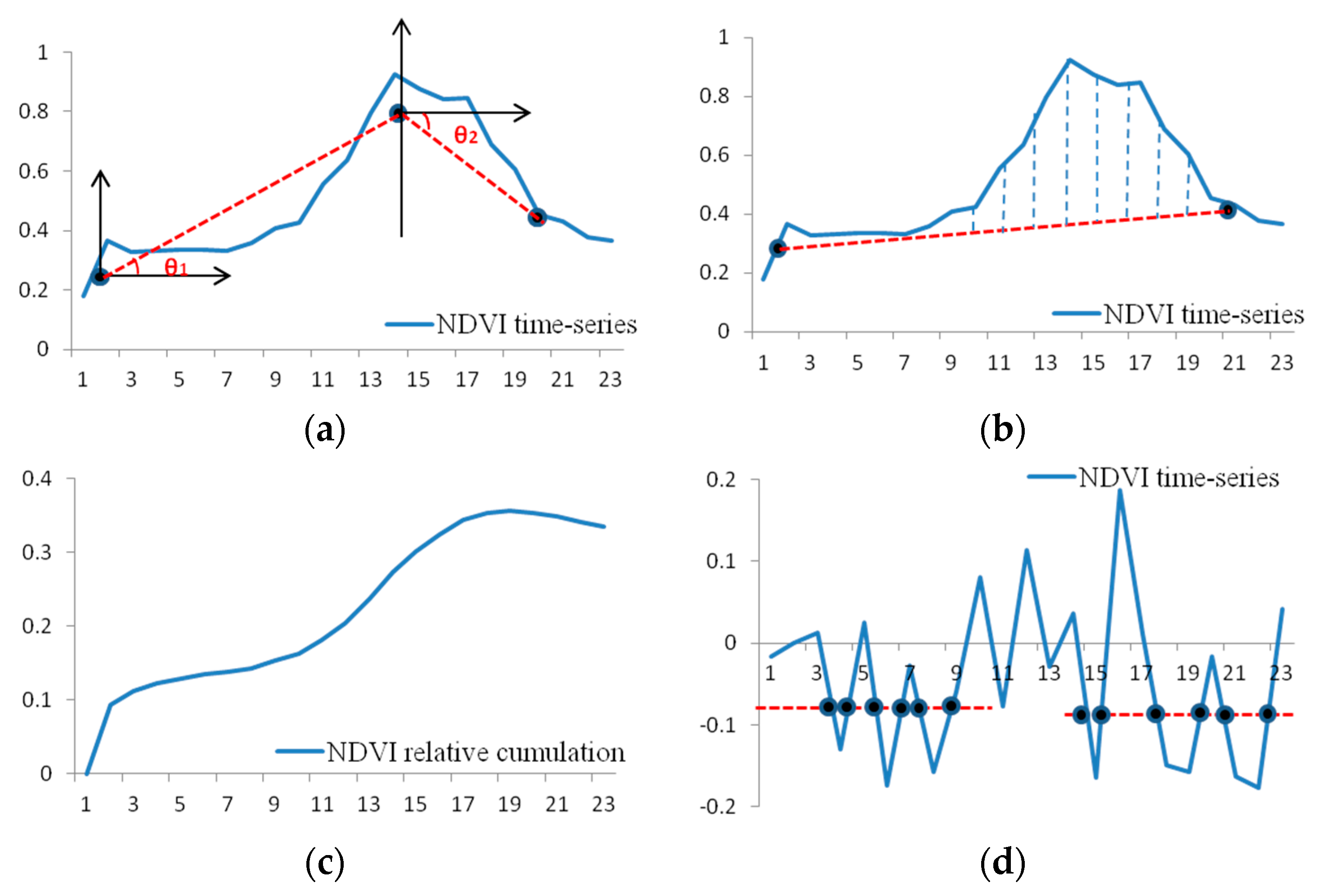
Phase angle cumulant (PAC). From the beginning of the year, the vegetation growth phases progress from vegetative growth to reproductive growth and withering [30]. The angle from one growth phase to another in the NDVI temporal curve was defined as the phase angle. It can be calculated with the NDVI changes and the time interval. As illustrated in Figure 2a, θ1 is the first phase angle and θ2 is the second phase angle of that NDVI temporal curve. Given n + 1 growth phases, n phase angles can be calculated from Equation (1), where V(i,e) and V(i,b) denote the ith NDVI values of the end phase and beginning phase, t(i,e) and t(i,b) denote the end and beginning time.
Baseline cumulant (BC). From the beginning of the growing season to its end, this period of NDVI time series acts as a measurement for most of the photosynthetic biomass accumulation. The straight line linking the beginning to the end of the growing season in the NDVI temporal curve was defined as the baseline. The baseline cumulant is defined by Equation (2), where ΔVi denotes the ith difference between the NDVI value and the baseline NDVI value, and B denotes the set of NDVI values above the baseline. The baseline is illustrated in Figure 2b.
Relative cumulation rate (RCR). Relative to the beginning of the growing season, the rates of the NDVI increase in the following time points represent a distinct absorption of near-infrared and infrared radiation for land cover types. The relative cumulation rate at a single time point is defined in Equation (3), where V0 denotes the value at the beginning of the growing season and Vi denotes the ith NDVI in the temporal curve composed of n NDVI values. The relative cumulation rate of the year is defined in Equation (4) as all rates of NDVI increase during one year:
Zero-crossing rate (ZCR). The zero-crossing rate is an indicator that reflects the fluctuations of a curve in a given time interval, and the properties of the curves can be estimated based on the short-time average zero-crossing rate [31]. This indicator plays an important role in automatic recognition systems which process signals that pass through the level of zero, especially in surface electromyogram spectral analysis, voiced classification, and other fields [31,32,33]. Because of natural or artificial disturbance, some land cover statuses change rapidly during a time interval. Therefore, the NDVI values show turbulent amplitude, resulting in a high zero-crossing count around a baseline. Figure 2d illustrates the zero-crossings around the baselines in two periods. The zero-crossing rate can be calculated with Equations (5) and (6), where T is the total time interval, Vi is the ith value of the NDVI temporal curve, and Vm denotes the mean value of the NDVI baseline during that period:
2.1.2. Spectral and Temporal Difference Calculation
For the bi-temporal multispectral images, Pearson’s correlation coefficient is adopted as a correlation operator to measure the similarity of two spectra [34]. The spectral change magnitude is calculated by Equation (7), where V is the reflectance of a pixel in band i, n is the band number, m denotes the mean value, and a and b denote the two spectra:
The differences of the shape parameters are calculated for the NDVI temporal curves from two years (the time series has an interval of 16 days in each year). The temporal change magnitudes are derived from Equation (8), where Δf is the difference of the same shape parameter in two years, p is the order, and n is the number of vectors in that shape parameter. After calculation, four change magnitude images of the NDVI shape parameters are generated.
2.2. Integration of Spectral–Temporal Change Magnitudes
2.2.1. Magnitude Normalization
The differences between bi-temporal multispectral images are measured with the spectral correlation operator and the spectral change magnitude is calculated by subtracting the correlation coefficient. Therefore, the unit of the spectral change magnitude is 1. For temporal change magnitudes derived from four independent shape parameters, the units are degree, value, or even ratio. The values of these parameters range widely and differ greatly each other. In consideration of integration, the units of these spectral and temporal change magnitudes should be unified into one form. Standard normalization is done to assimilate these change magnitudes. As shown in Equation (9), where M is the change magnitude, Mmin/Mmax is the minimum/maximum of the change magnitude among the whole gray image. The spectral and temporal change magnitudes are transformed into relative change magnitudes with a range between 0 and 1. Remarkably, this linear transformation formula converts the range into 0–1, which remains as the relative change level among the different land cover change types.
2.2.2. Integrating Spectral–Temporal Change Magnitude
The unified change magnitudes are integrated with a weighting function (as shown in Equation (10)), where w is a weighting factor, I is the unified change magnitude, and n is the number of all change magnitudes. In this study, the spectral correlation change magnitude and four temporal change magnitudes are adapted to calculate one spectral–temporal change magnitude with this weighting function.
2.3. Change Region Discrimination by Automated Thresholding
After the spectral–temporal change magnitude integration, a single change magnitude grey image is created. Many applications require a binary image which can be used to find change regions. To address this issue, a threshold selection method known as “the histogram concavity analysis” is adapted to provide a good candidate threshold for detecting the changed regions and unchanged regions in the grey image. By analysing the histogram’s concavity structure, this threshold selection method defines the optimal thresholds at the shoulders of the grey image histogram peaks [35]. Specifically, this method is an automated way to select a possible threshold. A more precise threshold may still need to be adjusted on the basis of this possible threshold. Then, comparing the grey image with the threshold, all regions that are greater than the threshold are detected as change regions.
3. Experiments
3.1. Study Area, Data Preprocessing, and Algorithm Implementation
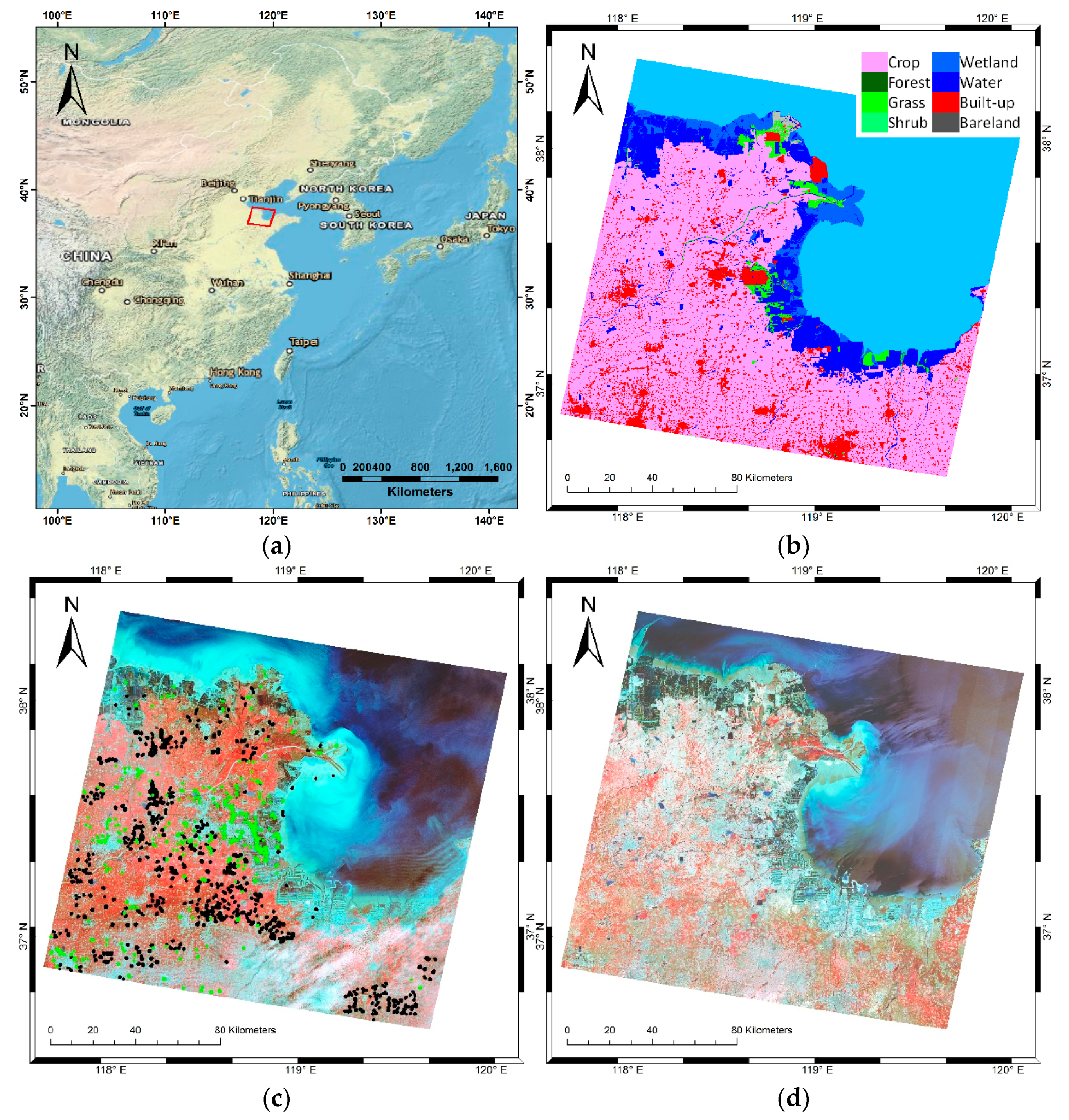
To test the performance of the proposed method, a case study was carried out in the northeast region (117°1′–120°34′ E, 36°8′–38°1′ N) of Shandong Province, China, as shown in Figure 3a. The average temperature of the study region is about 13 °C. This heat condition can satisfy the needs of the crop rotations. In addition, the average annual precipitation is about 555 mm, and the seasonal distribution of precipitation is uneven. Due to influences from biology, climate, and terrains, the soil is diversified in the region. Therefore, this study region has a variety of land cover types (main types are cropland, built-up, and water) as shown in Figure 3b, and the growths of different vegetation covers are varied. These natural factors and human disturbances such as wheat–corn rotation, urban expansion, and forest degradation cause uncertainty in the spectrum and NDVI temporal curves. All of these factors demand robust change detection methods.
Two Landsat images were downloaded (https://earthexplorer.usgs.gov) and transformed into the apparent reflectance (Figure 3c,d, the TM image consists of bands 1, 2, 3, 4, 5, and 7, the OLI image consists of bands 2, 3, 4, 5, 6, and 7). For the years 2010 and 2015, the NDVI time series drawn from the MODIS 16-day composite vegetation indices product (MOD13Q1) were obtained, totaling twenty-three NDVI images for each year (https://lpdaac.usgs.gov/data_access/data_pool). All of these NDVI images were projected from the sinusoidal projection to the WGS84 datum with the help of the MODIS reprojection tool (MRT). Then, the 30-m spatial resolution NDVI time series of 23 images in each year were reconstructed by the unmixing of these coarse NDVI time series [36,37,38,39]. The correlation coefficients of the generated fine NDVI time series and coarse NDVI time series were greater than 0.9 for each year. To evaluate the experimental results, the ground truth points (as shown in Figure 3c) were manually defined using the region of interest (ROI) tool from ENVI with the reference of high-resolution Google Earth images. Among these points, 2100 points had land cover conversions and 2523 points had no land cover conversions from the year 2010 to the year 2015. In the following, the change vector analysis is abbreviated as CVA, the image ratioing is abbreviated as IR; the spectral gradient-based change detection is abbreviated as SGD; the distance of Canberra is abbreviated as Dcanb, the NDVI gradient difference is abbreviated as NDVI-GD and the multiple shape parameter-based method is abbreviated as MSP.The methods of CVA, SGD, and IR used two Landsat images as inputs, NDVI-GD and Dcanb used two yearly fine NDVI time series as inputs. The MSP method used both two Landsat images and two yearly fine NDVI time series as inputs.
The MSP method was implemented with the IDL language and ran on a Windows 7 platform (Intel i3-3110M, 2 GB DDR3). The workflow was as follows (see Figure 1): (1) The spectral change magnitude image of the two Landsat images was calculated using Equation (6). (2) For PAC (as shown in Figure 2a), the y-axis values of the three points were set to mean values of 1–4, 11–21, and 20–23 of the NDVI time series, respectively, and the x-axis values were set to 2, 14, and 20, respectively. For BC (Figure 2b), the first point was set to the second NDVI point and the second point was set to the 22 NDVI point in the time series. For RCR (Figure 2c), V0 in Equation (3) was set to the first NDVI point in the time series. For ZCR (Figure 2d), Vm in Equation (6) of the first baseline was set to the means of the 1st to 13th NDVI values in the time series. The Vm of the second baseline was set to the means of the 13th to 23rd NDVI values in the time series. The T in Equation (5) was set to 23. Based on these settings, each shape parameter of the NDVI temporal curves was calculated. Four temporal change magnitude images were calculated in Equation (8), with p being 2 for RCR and 1 for other parameters. (3) All of the change magnitude images were integrated into one single change magnitude image, making every w equal to 1 in Equation (10). (4) The histogram of the change magnitude image was analyzed to select a threshold at the shoulders of the histogram peaks, and the change regions were discriminated by comparing them with this threshold.
3.2. Results
3.2.1. Change Magnitudes in the Ground Truth Points
In general, the change magnitudes in the real changed regions should have higher responses than in unchanged regions. The difference of the change magnitudes between the changed and unchanged regions could reflect the contrast quantitatively. Based on the two ground truth points group (one consisting of 2100 changed ground truth points, another consisting of 2523 unchanged ground truth points), the mean and median of the change magnitudes in each group and the standard deviation in all 4623 points were calculated. The differences between the changed and unchanged groups are listed in Table 1 with the units of percentage, and the standard deviation given separately. The difference from MSP was greater than the other compared methods. For MSP, the change magnitudes in the changed points were higher than in the unchanged points. This indicates that the MSP could generate high-contrast change magnitudes, which makes the discrimination of changes and no-changes easier.
3.2.2. Change Magnitude Images
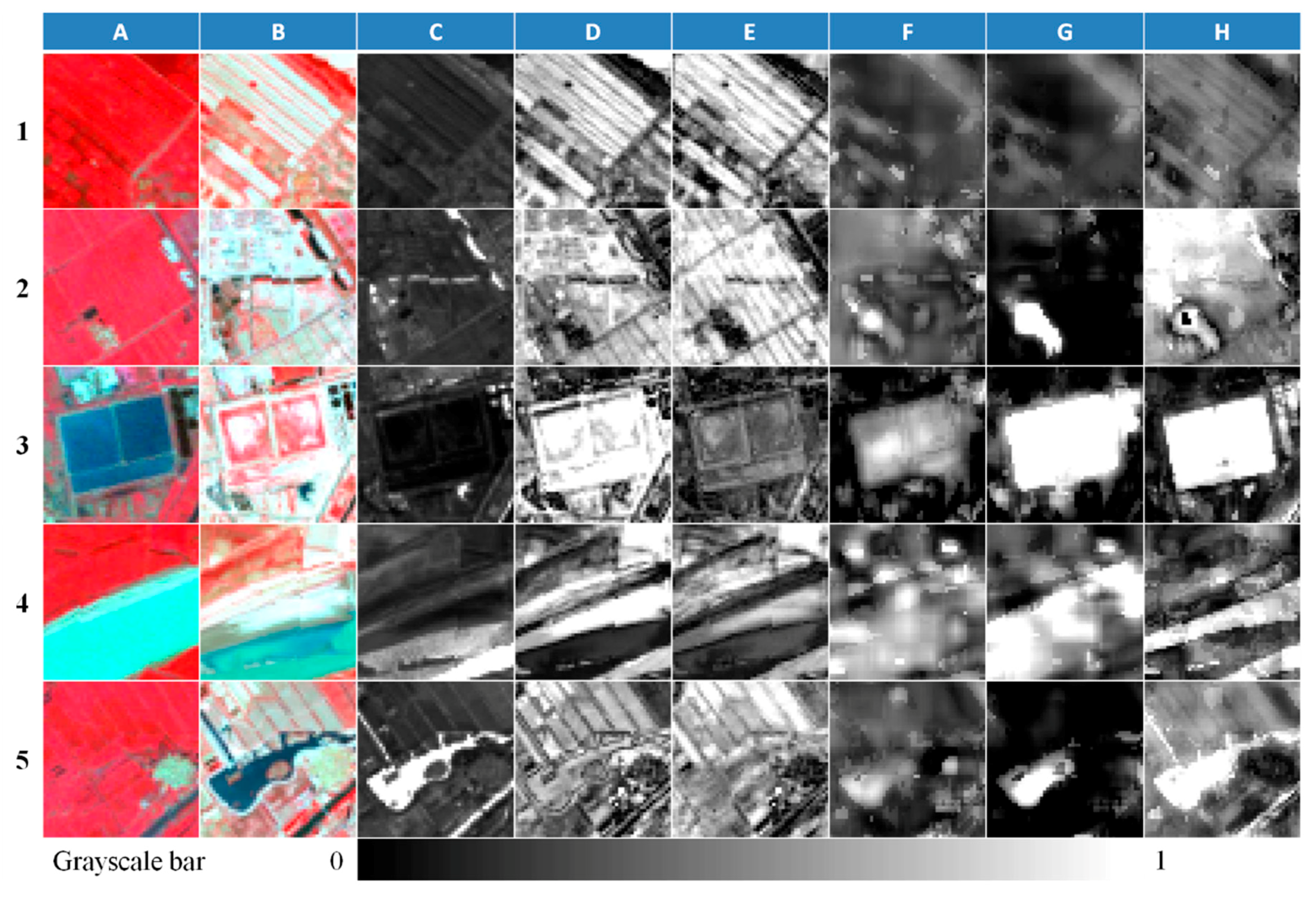
From 2010 to 2015, five conversions of land cover types in the study area are given with subareas in Figure 4. They are: (1) from crop in growth to crop in harvest; (2) from crop in growth to built-up; (3) from water to vegetation; (4) from muddy water to bare land; and (5) from crop to water. All these change magnitudes were normalized linearly to facilitate visual comparison and brightness is used to indicate change possibility.
In the Landsat image, the crop type shows a strong difference from the growing season (red) to the harvest season (white). Results of CVA and SGD showed high change magnitudes, while results from IR, NDVI-GD, and Dcanb showed low change magnitudes. The results of the MSP showed moderate but relatively low change magnitudes compared to the others. Because of urban expansion, some parts of the crop areas in 2010 were converted to built-up in 2015, while other parts remained as crop type, but after the harvesting. MSP results showed strong change magnitudes in the changed areas (crop to built-up) and light change magnitudes in the no-change areas (crop in growth to crop in harvest). This gave a great contrast between the change and no-change scenarios in the change magnitude image. The results of IR, CVA, and SGD were indistinguishable, while NDVI-GD and Dcanb were able to distinguish between changes and no-changes. However, they were not distinct enough. When water changed to vegetation, the MSP results showed a clear boundary between the changes and no-changes as shown in the Row 3 of Figure 4. When the yellow river shifted its path over five years, a part of the riverbed on one side was bare and a part of the other side was occupied by crops. The results of MSP gave a strong response to this change (from muddy water to bare land) and a light response to the no-change regions (from crop in growth to crop in harvest). The results of other methods were either indistinguishable or lacked the texture detail necessary to distinguish them accurately. In the case of crop to water, the advantage of keeping the texture detail of the real changes and abandoning no-changes was obvious for the MSP method.
3.2.3. Change Regions
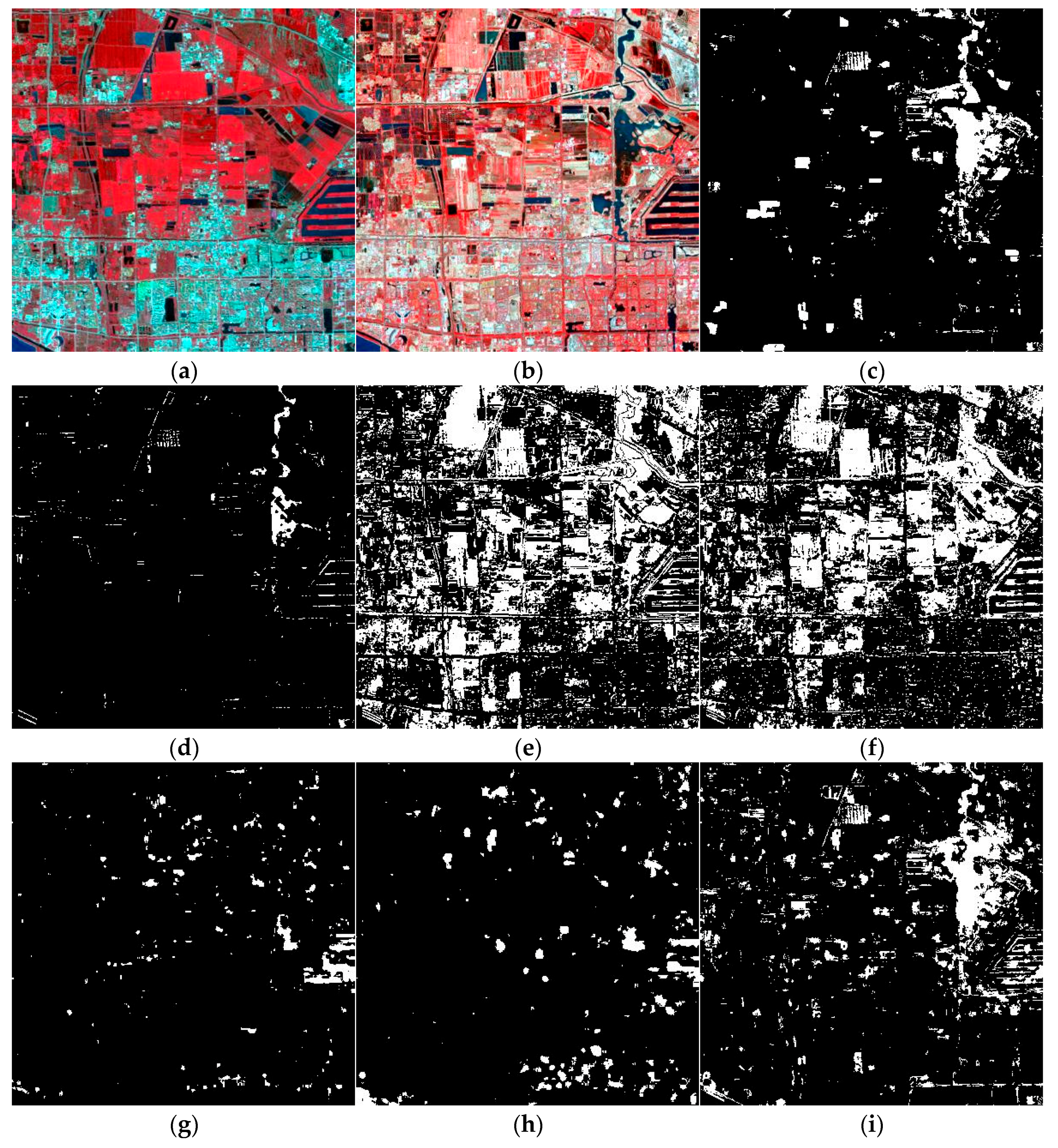
The change magnitude images calculated from all test change detection methods were divided into changes and no-changes expressed with binary images, where the change is symbolized as white and the no-change is symbolized as black. All thresholds were automatically derived from the histogram concavity analysis. The ground truth image of the change regions was extracted interactively using the ROI tool from ENVI and Google Earth images. Partial change detection results of the study area are shown in Figure 5. It shows that the change result of MSP was closer to the ground truth image than other methods. Bi-temporal image-based change detection methods such as IR, CVA, and SGD could not provide accurate change results because of the phenological difference in multispectral Landsat images. Based on the 30-m NDVI time series, the pseudo-changes in the former were reduced (Figure 5g,h). However, some parts of the real changes were missing in the final change results of Dcanb and NDVI-GD. Due to the change magnitudes, these two methods had a low-contrast difference (Figure 4) and it is difficult for an automated threshold selection method to accurately discriminate the real changes from no-changes. In contrast, the MSP results were more accurate in these conditions.
3.2.4. Accuracy Assessment
The overall accuracy of the change detection result of MSP was 88.427% and the kappa coefficient was 0.764, as shown in Table 2. A comparison of the overall accuracy and kappa coefficient was also made for the other five change detection methods associated with the automated threshold, respectively, as shown in Table 3. The overall accuracy and kappa coefficient of MSP tended to be higher than those of the other five methods in this study area, indicating that the MSP change result derived from the automated threshold was more reliable and appropriate than the other methods. This advantage is especially important in automated change detection projects.
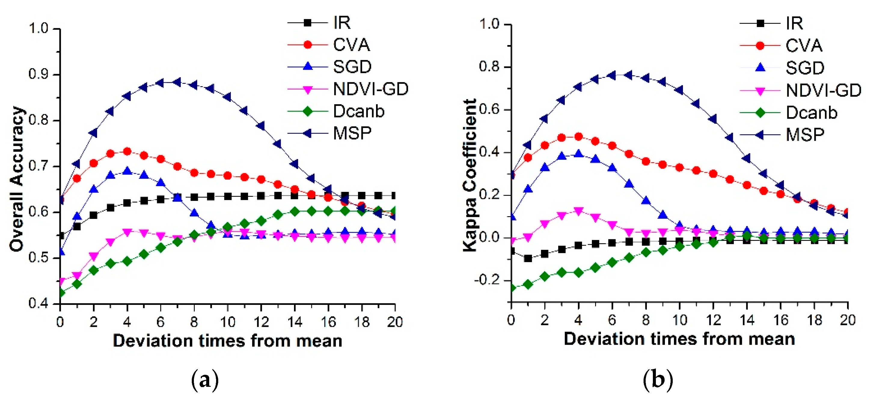
In addition, accuracy assessment curves were made to compare the performance of all six methods at different threshold levels. Based on the accuracy assessment curves, the relationship between the threshold levels and accuracies can be presented graphically [40]. In Figure 6, a series of thresholds which were converted into the deviation times of the standard deviation from the mean of the change magnitudes with a step of 0.25 are arranged on the x-axis. From the chart of the overall accuracy in Figure 6a and the chart of the kappa coefficient in Figure 6b, MSP achieved the highest levels in a wide range. With a threshold at seven deviations, MSP reached a peak (overall accuracy was about 88% and the kappa coefficient was about 0.76). Then, the accuracies declined gradually with the increase of the threshold levels. The other five methods showed a poor performance over the whole scene in the study area. CVA, SGD, and NDVI-GD reached a peak at four deviations for both the overall accuracy and the kappa coefficient. IR and Dcanb increased gradually along with the threshold levels and reached a best overall accuracy of 0.65. The kappa coefficients of these two methods were low throughout the entire range. This comparison indicates that MSP was effective in a wide range of thresholds and could simultaneously achieve the best overall accuracy and kappa coefficient.
4. Discussion
4.1. The Influence of Different Order p on Change Magnitudes and Accuracy
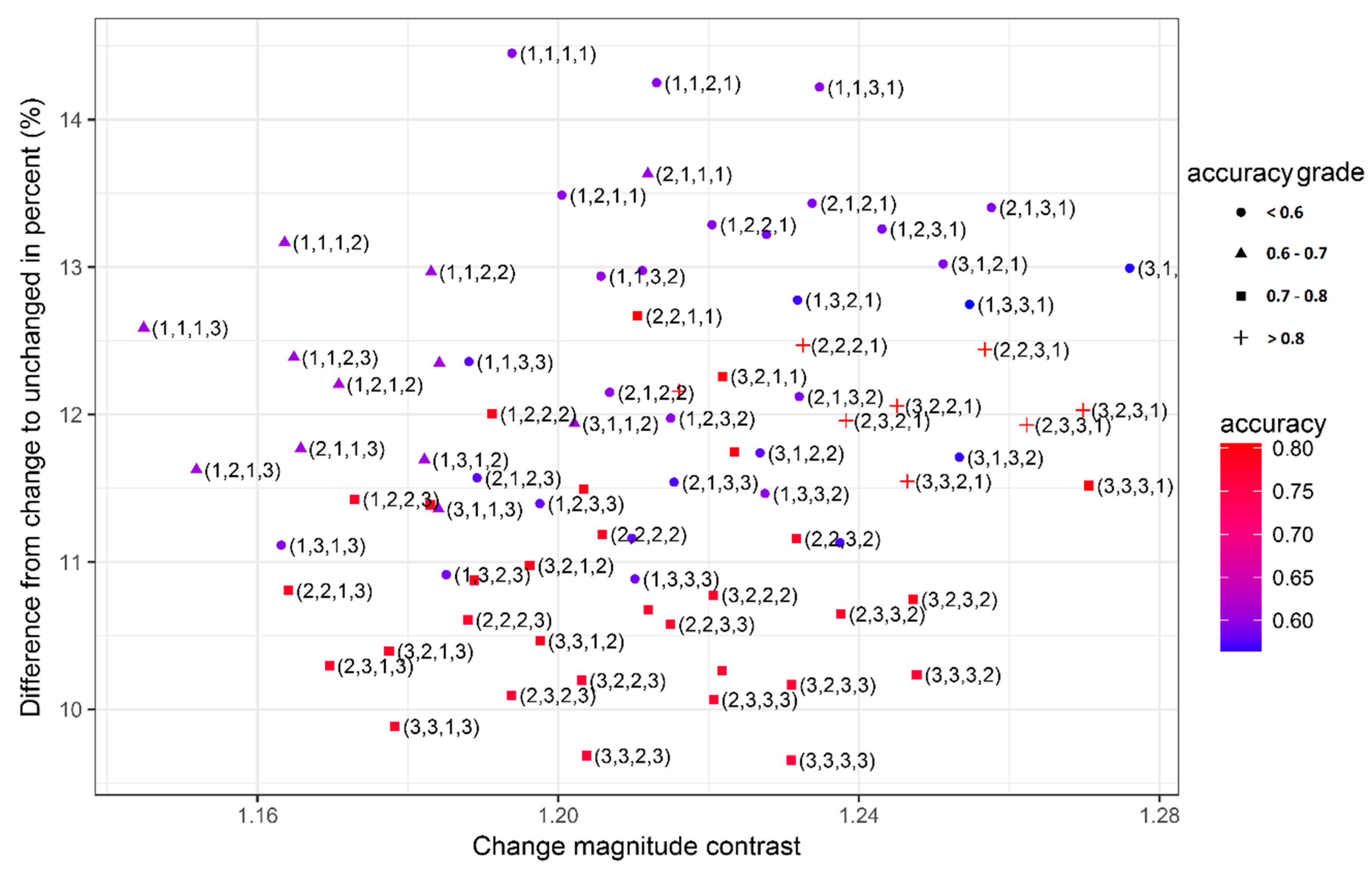
The change magnitudes of the NDVI time series are calculated based on PAC, BC, RCA, and ZCR in MSP. The order p in Equation (8) determines the differences of all these temporal change magnitudes (assuming p1, p2, p3, and p4 were of the order p when calculating the differences of PAC, BC, RCA, and ZCR, respectively). Therefore, the contrast between the changed and unchanged pixels (abbreviated as CCU), the difference between the changed and unchanged pixels (abbreviated as DCU) in the change magnitude of MSP, and the overall accuracy will be affected by the various combinations of the order p. In this section, the values 1, 2, and 3 were assigned to p1, p2, p3, and p4, and a total of 81 (34) combinations were selected to test their influence on the contrast, the difference between changed and unchanged pixels, and the overall accuracy (every weighting factor w was set to 1). As shown in Figure 7, the DCU of combinations ((1, 1, 1, 1), (1, 1, 2, 1), and (1, 1, 3, 1)) were high and the CCU of combinations ((3, 2, 3, 1), (2, 3, 3, 1), and (3, 3, 3, 1)) were also high. Although the higher DCU and CCU could show a high-contrast change magnitude, it is clear that the highest DCU and CCU did not bring the highest accuracy. From the scattered points in Figure 7, we can see that the combinations (2, 2, 3, 1), (3, 2, 3, 1), and (2, 3, 3, 1) are superior for DCU, CCU, and accuracy.
4.2. The Functions of the Weighting Factor w in the Integration
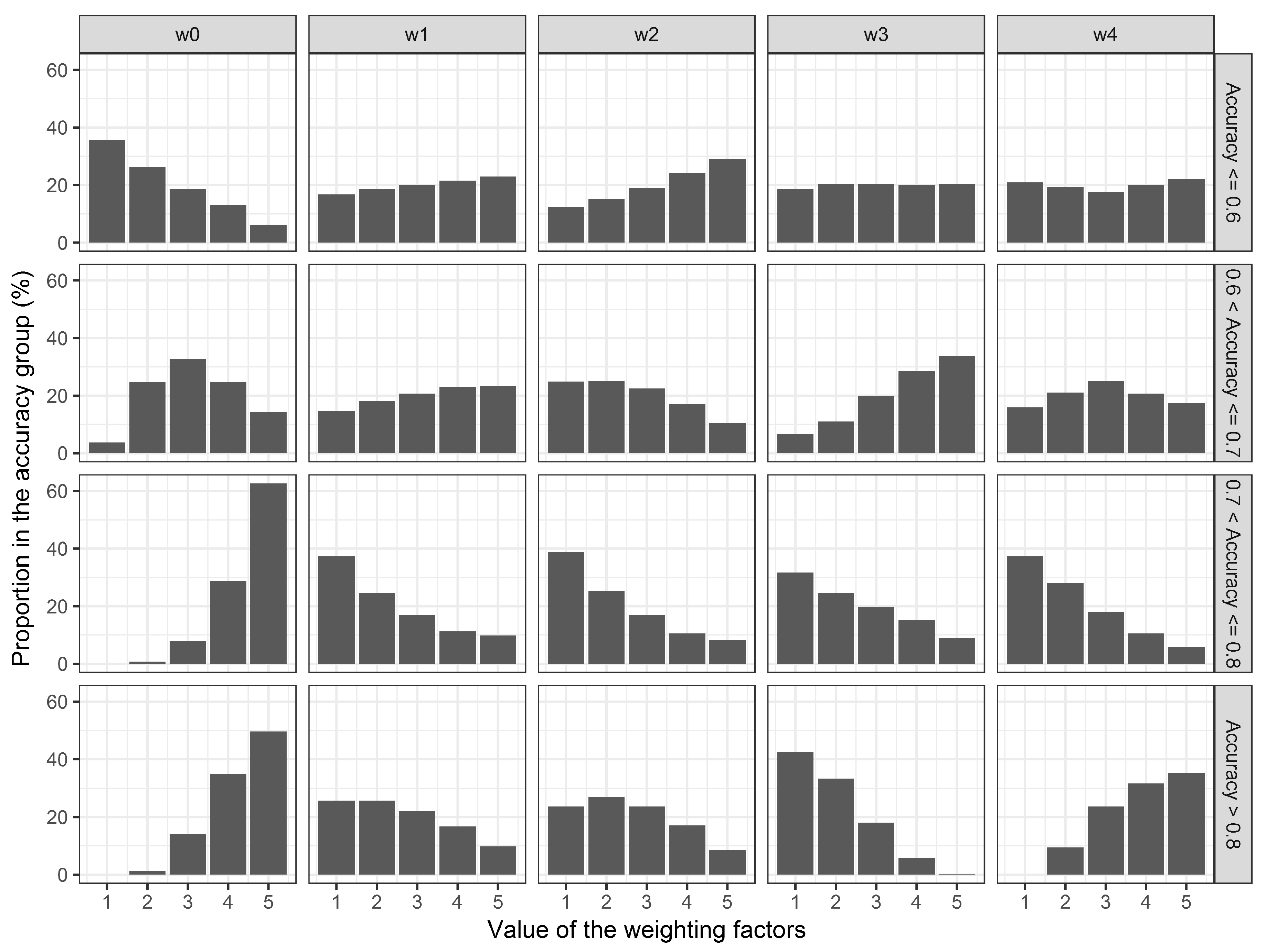
The change magnitudes of the proposed shape parameters describe the differences between the land cover conversions in several dimensions. The weighting factors of these change magnitudes determine the proportions of particular change magnitudes in the final MSP change magnitude, and thus, they affect the final change detection accuracy. Values from 1 to 5 were assigned to each weighting factor w, and the overall accuracies of MSP change detection under 3125 (55) combinations of all five factors were calculated (every p was set to 1). Figure 8 gives the value distributions of the w factor in the different accuracy groups, where w0, w1, w2, w3, and w4 are the weighting factors of the change magnitudes of SC (spectral correlation), PAC, BC, RCR, and ZCR, respectively. The figure shows that w0 gradually moved from 1 to 5 as accuracy increased. In the groups in which the accuracy was greater than 0.7, most w0 values were 5. The value distributions of w1 and w2 were similar when the accuracy was greater than 0.7. The values 1, 2, and 3 are advisable for w1 and w2 to achieve a higher accuracy. Based on the value distributions of w3, the value shifted sharply from 5 to 1 as the increasing of accuracy. The preferred values of w3 were 1 and 2. When accuracy was greater than 0.8, it is clear that most of w4 gathered around the weighting factor value of 5, and the proportions of w4 in values 4 and 5 were close to each other. Therefore, weighting factor values of 4 and 5 are recommended for w4. It seems that the combinations of (w0, w1, w2, w3, w4) set as (5, 1/2/3, 1/2/3, 1/2, 4/5) could achieve a higher overall accuracy. The accuracy of all these combinations was greater than 0.78, and 49% of them were greater than 0.8.
4.3. Change Detection with a Single Shape Parameter
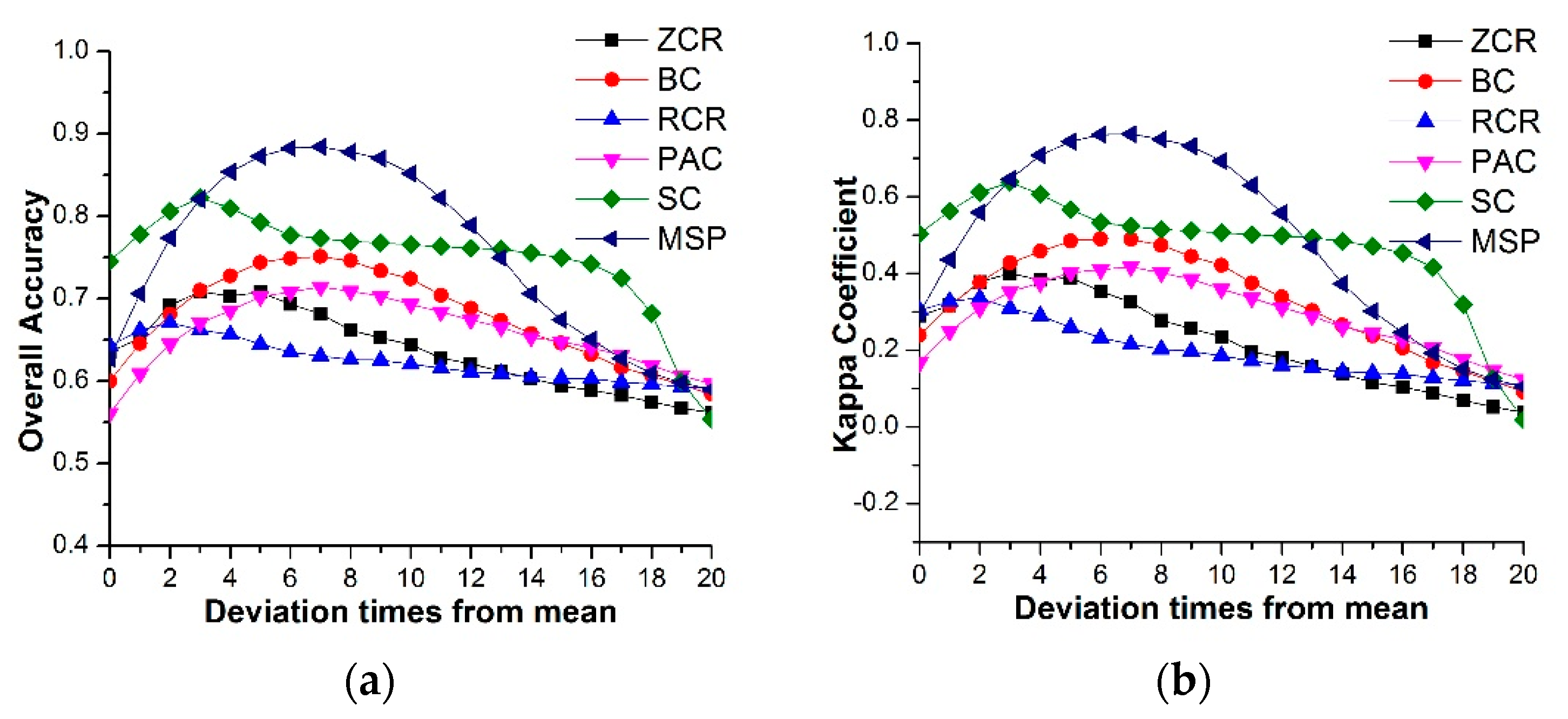
The proposed shape parameters can be used independently to perform change detection. Figure 9 shows the accuracy assessment curves of these indicators with MSP as a comparison. Based on the spectral characteristic of the Landsat image, spectral correlation performed better than NDVI temporal curve-based shape parameters. The baseline cumulant achieved an overall accuracy of 0.75, which was the highest level using the NDVI time series separately. However, the overall accuracy and kappa coefficient of these separate indicators were lower than MSP in a wide range, from 3 to 13. Although the accuracy of each shape parameter was low for most thresholds, the overall accuracy of MSP was greater than 0.8. This indicates that the integration of these separate shape parameters improves the accuracy of the final change detection results. Each of them contributes to the accuracy of integration to varying degrees.
4.4. The Contributions of Shape Parameter to Land Cover Conversions
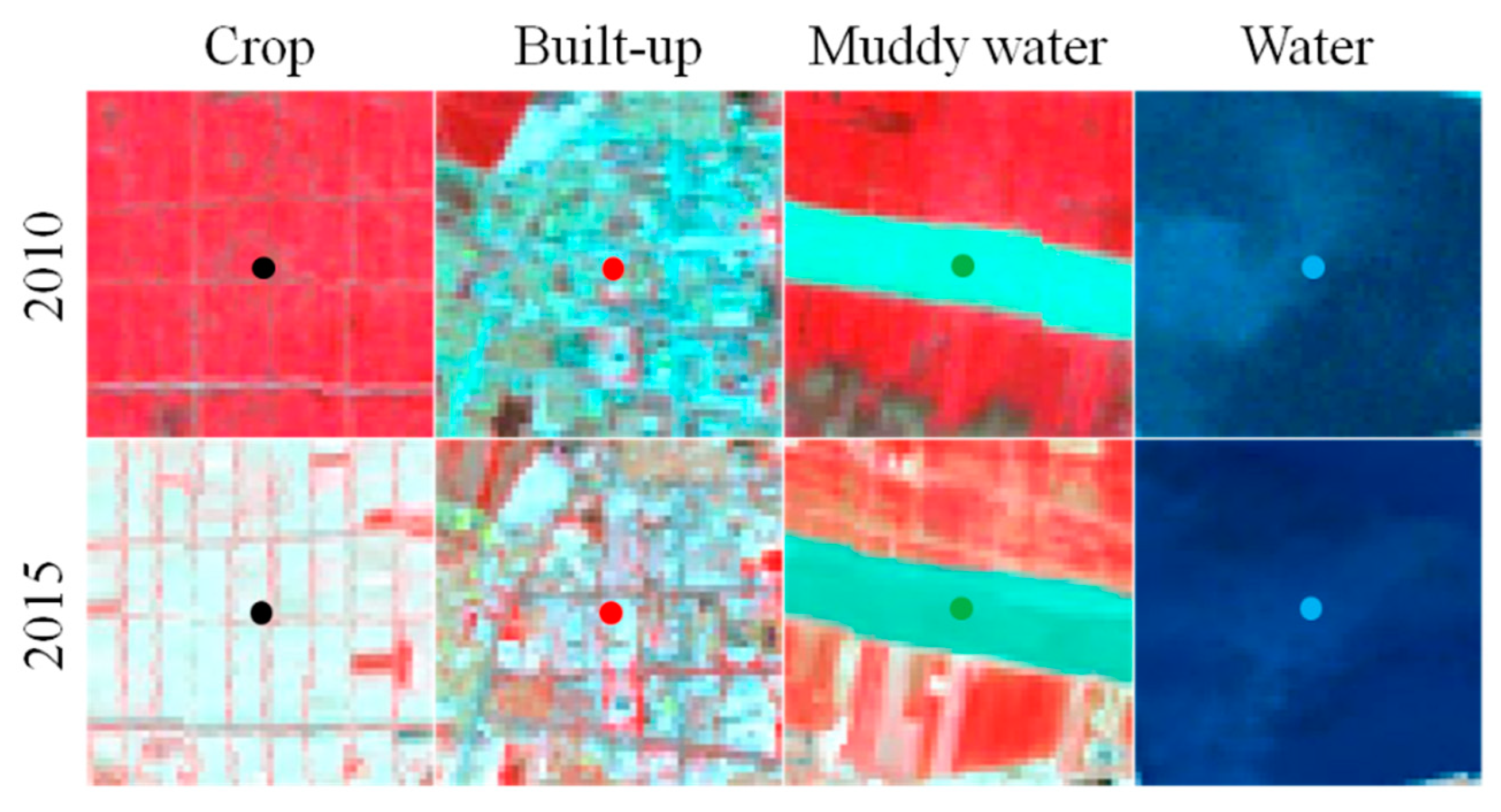
As mentioned in Section 3.1, land cover types such as crop, built-up, and water were dominant in the study area. Therefore, the functions of each shape parameter in the conversions between these land cover types should be major concerns. The spectrum and 30-m NDVI time series of four land cover types (crop, built-up, muddy water, and water) were sampled with a pixel point in years 2010 and 2015, as shown in Figure 10. The change magnitudes of these land cover conversions were calculated using each shape parameter and normalized linearly to range between 0 and 1.
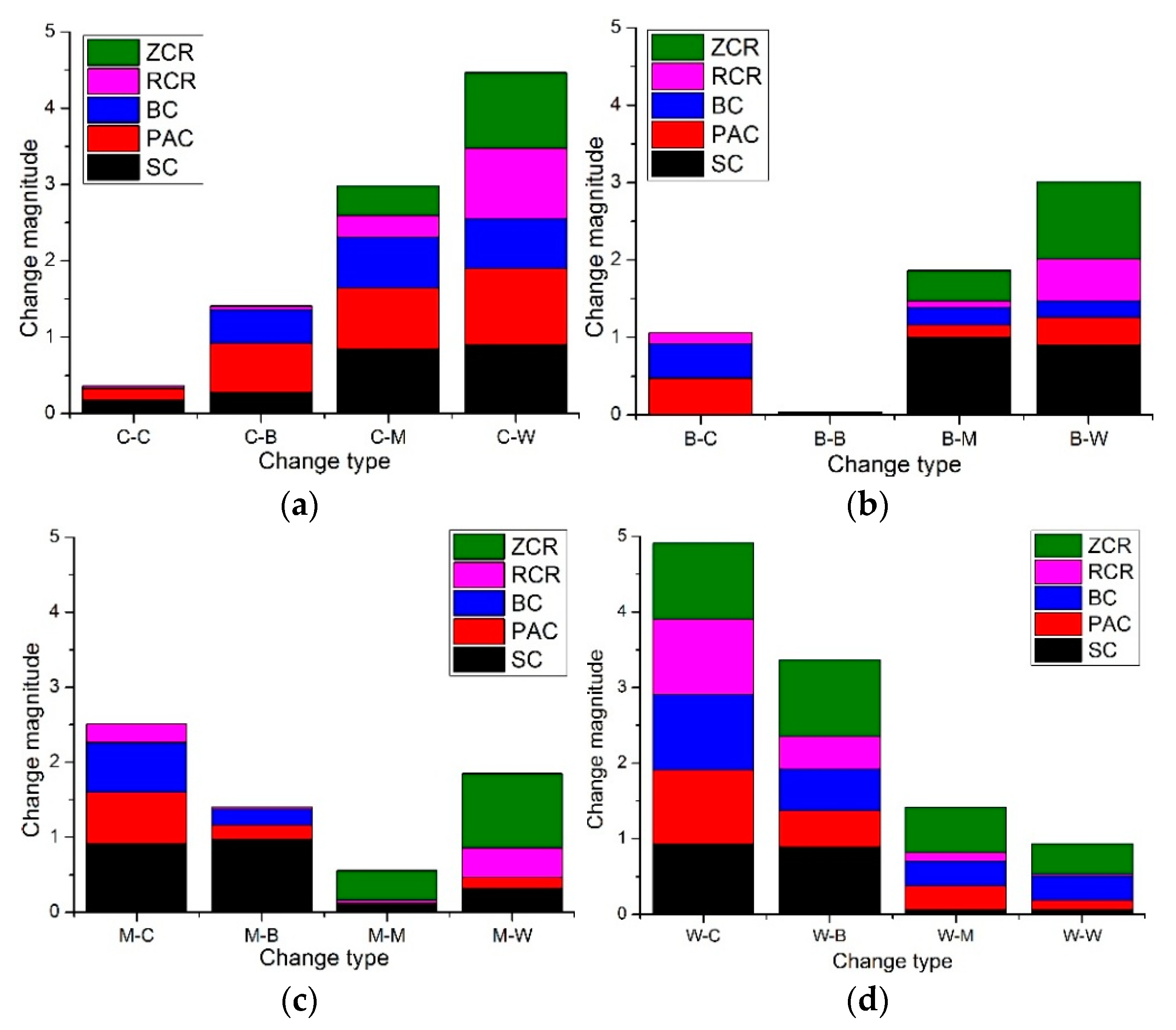
The land cover types crop, built-up, muddy water, and water are abbreviated as C, B, M, and W, respectively, in Figure 11. The conversions from 2010 to 2015 are expressed as “type-type” in the following. In the case of conversions from crop to other types, as shown in Figure 11a, the baseline cumulation contributed a high change magnitude to changes and low change magnitude to no-changes. The following is the relative cumulation rate, which performed effectively for no-changes. The phase angle gave a high contrast between changes and no-changes. The spectral correlation gave a low contrast between C-C and C-B. The zero-crossing rate performed well in conversions with water or muddy water. As shown in Figure 11b, in the case of built-up to others, baseline cumulation, phase angle, and relative cumulation rate worked together to give a high change magnitude in B-C. The zero-crossing rate and spectral correlation enhanced the change magnitudes of B-M and B-W, which was weak in B-M. In the case of changes from muddy water to other types, as shown in Figure 11c, the spectral correlation performed well, but not strongly enough to highlight the changes among M-M and M-W. The phase angle gave the lowest change magnitude. The rest were complementary to improve the magnitude of changes. In the case of changes from water to other types, as shown in Figure 11d, the zero-crossing rate gave a high contrast between changes and no-changes. Baseline cumulation performed poorly between W-M and W-W, as did the phase angle between W-B and W-M. Similarly, the relative cumulation rate did not work in discriminating W-M and W-W. Despite these shortcomings, the final change magnitude was enhanced by the integration of different change magnitudes.
4.5. The Applicability of Data Quality for Landsat Images and NDVI Time Series
Previous research has demonstrated that multi-spectral images should be pre-processed by radiometric and atmospheric correction for quantitative remote sensing applications [41,42,43]. For the purpose of land cover change detection, some researchers have argued that this type of pre-processing is unnecessary in cases where the images are acquired under the same imaging conditions. Noise reduction techniques for NDVI time series have been widely used to improve the monitoring ability of vegetation dynamics. Therefore, the pre-processing changes the data quality of Landsat images or NDVI time series by reducing the difference of radiation or phenology. The applicability of the proposed method for various inputs is important for its wide range of application.
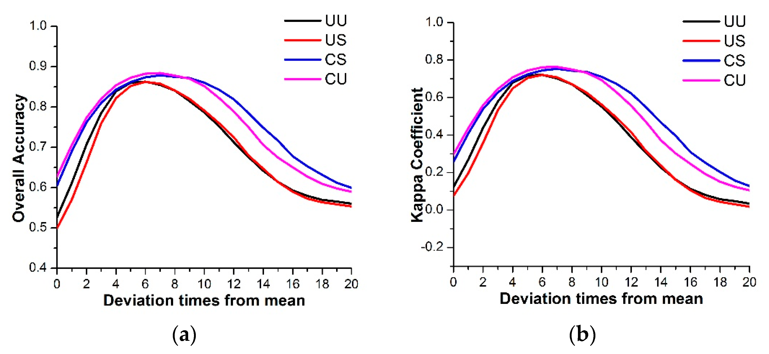
Two kinds of Landsat images (under radiometric correction or both radiometric and atmospheric correction) and two kinds of NDVI time series (with the Savitzky–Golay filter applied or without it) were taken as inputs for MSP. Figure 12 shows that the accuracies of UU and US (UU denotes data with no atmosphere correction and no Savitzky–Golay filter; US denotes data with no atmosphere correction and with the Savitzky–Golay filter) were lower than CS and CU (CS denotes data with atmosphere correction and the Savitzky–Golay filter; CU denotes the data with atmosphere correction and without the Savitzky–Golay filter). This indicates that atmosphere correction is vital for MSP. When atmosphere correction was performed, the accuracy reached a higher level, as seen by the blue and pink curves in Figure 12. When the thresholds were lower than nine times the deviation, the mean of the change magnitudes was selected to detect the changes and the Savitzky–Golay filtering was not necessary. By increasing the thresholds, the Savitzky–Golay filtering becomes important to obtain a high accuracy. This result indicates that using Landsat images after atmosphere correction is essential for MSP and the filtering of the NDVI time series is not indispensable.
5. Conclusions
In order to calculate a high-contrast change magnitude, a novel change detection method based on multiple shape parameters is proposed in this study. As demonstrated in the experiments, the shape parameters of the NDVI temporal curve and spectrum could be used to detect the inter-annual land cover conversions. These shape parameters were from reconstructions of phenological parameters, existing indicators, and mathematical indexes. Some of them were shown to be effective in particular transformations of land cover types. For example, the zero-crossing rate was valid for detecting the fluctuation of the NDVI temporal curve of water. The phase angle cumulant showed an obvious effect in transformations having crop types. However, none of them was more powerful than the others obviously in detecting various land cover conversions. After the integration of these shape parameters, a high-contrast change magnitude image could be calculated. MSP’s change magnitude of the NDVI temporal curve is derived from the annual change characteristics during the whole year rather than the accumulation of the NDVI differences in each single time point of the year. Accordingly, the offset between the different conflicting differences of single time points is avoided and the changes show a higher response compared with the no-change scenario. Therefore, pseudo-changes are reduced further and the real changes and non-changes are more easily discriminated.
The result of the case study showed that an overall accuracy of about 88% was achieved by MSP, and its kappa coefficient was 0.76. The change regions in the change magnitudes of dominant land covers were distinguishable, which could provide a broad range to the set thresholds. This property is important to detect changes accurately among the various change types. The change magnitude images were distinct from the main land cover conversions in the study area, which ensured that the change regions and no-change regions had a high-contrast. The pseudo-changes caused by the phenological differences of the Landsat images could be eliminated further. This means that we might be able to conclude that MSP is feasible for land cover change detection in regions suffering from pseudo-change errors. The MSP maintained high accuracies in a wide range of threshold levels and depends less on filtering. This might demonstrate that MSP is robust for either automated or optional change detection projects.
The MSP method also has disadvantages. Firstly, this method needs both bi-temporal Landsat images and 30-m NDVI time series as inputs, which is a restriction for some land cover change detection programs that lack these datasets. Another limitation is the low efficiency compared to traditional direct comparison-based change detection methods. Several change magnitudes derived from multiple shape parameters should be calculated separately and integrated into one in MSP. Third, MSP only calculates a binary change image, cannot provide a “from–to” image, and lacks the ability to detect changes within one year. In the future, fewer but more effective features of NDVI temporal curves might be a possible way to improve its efficiency. Due to the many parameters that are involved in MSP, more research needs to be done to identify their detailed function. It would also be valuable to perform the MSP method based on image objects.
Author Contributions
B.L. developed the concept, designed and implemented the method, performed the experiments, and drafted the first manuscript. J.C. (Jun Chen) made substantial contributions to the conceptual design and preparation of the manuscript. J.C. (Jiage Chen) and W.Z. participated in the project discussions and performed part of the revision.
Funding
This research was funded by the National Natural Science Foundation of China (Grant No. 41231172 and No. 41701477).
Acknowledgments
The authors would like to thank Jin Chen and Xuehong Chen for their advice and thank anonymous reviewers for their effort and insight.
Conflicts of Interest
The authors declare no conflict of interest.
References
- Cihlar, J. Land cover mapping of large areas from satellites status and research priorities. Int. J. Remote Sens. 2000, 21, 1093–1114. [Google Scholar] [CrossRef]
- Friedl, M.A.; McIver, D.K.; Hodges, J.C.F.; Zhang, X.Y.; Muchoney, D.; Strahler, A.H.; Woodcock, C.E.; Gopal, S.; Schneider, A.; Cooper, A.; et al. Global land cover mapping from modis: Algorithms and early results. Remote Sens. Environ. 2002, 83, 287–302. [Google Scholar] [CrossRef]
- Hansen, M.C.; Potapov, P.V.; Moore, R.; Hancher, M.; Turubanova, S.A.; Tyukavina, A.; Thau, D.; Stehman, S.V.; Goetz, S.J.; Loveland, T.R.; et al. High-resolution global maps of 21st-century forest cover change. Science 2013, 342, 850–853. [Google Scholar] [CrossRef] [PubMed]
- Lu, D.; Mausel, P.; Brondízio, E.; Moran, E. Change detection techniques. Int. J. Remote Sens. 2004, 25, 2365–2401. [Google Scholar] [CrossRef]
- Singh, A. Digital change detection techniques using remotely-sensed data. Int. J. Remote Sens. 1989, 10, 989–1003. [Google Scholar] [CrossRef]
- Hansen, M.C.; Loveland, T.R. A review of large area monitoring of land cover change using landsat data. Remote Sens. Environ. 2012, 122, 66–74. [Google Scholar] [CrossRef]
- Coppin, P.; Jonckheere, I.; Nackaerts, K.; Muys, B.; Lambin, E. Digital change detection methods in ecosystem monitoring: A review. Int. J. Remote Sens. 2004, 25, 1565–1596. [Google Scholar] [CrossRef]
- Mas, J.-F. Monitoring land-cover changes: A comparison of change detection techniques. Int. J. Remote Sens. 1999, 20, 139–152. [Google Scholar] [CrossRef]
- Xing, H.; Chen, J.; Wu, H.; Zhang, J.; Li, S.; Liu, B. A service relation model for web-based land cover change detection. ISPRS J. Photogram. Remote Sens. 2017, 132, 20–32. [Google Scholar] [CrossRef]
- Thonfeld, F.; Feilhauer, H.; Braun, M.; Menz, G. Robust change vector analysis (RCVA) for multi-sensor very high resolution optical satellite data. Int. J. Appl. Earth Observ. Geoinf. 2016, 50, 131–140. [Google Scholar] [CrossRef]
- Mouat, D.A.; Mahin, G.G.; Lancaster, J. Remote sensing techniques in the analysis of change detection. Geocarto Int. 1993, 8, 39–50. [Google Scholar] [CrossRef]
- Coppin, P.R.; Bauer, M.E. Digital change detection in forest ecosystems with remote sensing imagery. Remote Sens. Rev. 1996, 13, 207–234. [Google Scholar] [CrossRef]
- Malila, W.A. Change vector analysis an approach for detecting forest changes with landsat. In LARS Symposia; Purdue University: West Lafayette, IN, USA, 1980; p. 385. [Google Scholar]
- Chen, J.; Gong, P.; He, C.; Pu, R.; Shi, P. Land-use /land-cover change detection using improved change-vector analysis. Photogram. Eng. Remote Sens. 2003, 69, 369–379. [Google Scholar] [CrossRef]
- Bovolo, F.; Bruzzone, L. A theoretical framework for unsupervised change detection based on change vector analysis in the polar domain. IEEE Trans. Geosci. Remote Sens. 2006, 45, 218–236. [Google Scholar] [CrossRef]
- Yuhas, R.H.; Goetz, A.F.H.; Boardman, J.W. Discrimination among semi-arid landscape endmembers using the spectral angle mapper (SAM) algorithm. In JPL, Summaries of the Third Annual JPL Airborne Geoscience Workshop; NASA: Washington, DC, USA, 1992; Volume 1, pp. 147–149. [Google Scholar]
- Kruse, F.A.; Lefkoff, A.B.; Boardman, J.W.; Heidebrecht, K.B.; Shapiro, A.T.; Barloon, P.J.; Goetz, A.F.H. The spectral image processing system (SIPS)-interactive visualization and analysis of imaging spectrometer data. Remote Sens. Environ. 1993, 44, 145–163. [Google Scholar] [CrossRef]
- Chen, J.; Lu, M.; Chen, X.; Chen, J.; Chen, L. A spectral gradient difference based approach for land cover change detection. ISPRS J. Photogram. Remote Sens. 2013, 85, 1–12. [Google Scholar] [CrossRef]
- Jonsson, P.; Eklundh, L. Timesat—A program for analyzing time-series of satellite sensor data. Comput. Geosci. 2004, 30, 833–845. [Google Scholar] [CrossRef]
- Bradley, B.A.; Jacob, R.W.; Hermance, J.F.; Mustard, J.F. A curve fitting procedure to derive inter-annual phenologies from time series of noisy satellite NDVI data. Remote Sens. Environ. 2007, 106, 137–145. [Google Scholar] [CrossRef]
- Jakubauskas, M.E.; Legates, D.R.; Kastens, J.H. Crop identification using harmonic analysis of time-series avhrr NDVI data. Comput. Electron. Agric. 2002, 37, 127–139. [Google Scholar] [CrossRef]
- Buyantuyev, A.; Wu, J. Urbanization diversifies land surface phenology in arid environments: Interactions among vegetation, climatic variation, and land use pattern in the Phoenix metropolitan region, USA. Landsc. Urban Plan. 2012, 105, 149–159. [Google Scholar] [CrossRef]
- Tucker, C.J.; Justice, C.O.; Prince, S.D. Monitoring the grasslands of the sahel 1984–1985. Int. J. Remote Sens. 1986, 7, 1571–1581. [Google Scholar] [CrossRef]
- Shimabukuro, Y.E.; Holben, B.N.; Tucker, C.J. Fraction images derived from noaa avhrr data for studying the deforestation in the brazilian amazon. Int. J. Remote Sens. 1994, 15, 517–520. [Google Scholar] [CrossRef]
- Lunetta, R.S.; Knight, J.F.; Ediriwickrema, J.; Lyon, J.G.; Worthy, L.D. Land-cover change detection using multi-temporal modis NDVI data. Remote Sens. Environ. 2006, 105, 142–154. [Google Scholar] [CrossRef]
- Klein, I.; Gessner, U.; Kuenzer, C. Regional land cover mapping and change detection in central Asia using modis time-series. Appl. Geogr. 2012, 35, 219–234. [Google Scholar] [CrossRef]
- Chen, X.; Yang, D.; Chen, J.; Cao, X. An improved automated land cover updating approach by integrating with downscaled NDVI time series data. Remote Sens. Lett. 2015, 6, 29–38. [Google Scholar] [CrossRef]
- Lu, M.; Chen, J.; Tang, H.; Rao, Y.; Yang, P.; Wu, W. Land cover change detection by integrating object-based data blending model of landsat and modis. Remote Sens. Environ. 2016, 184, 374–386. [Google Scholar] [CrossRef]
- Reed, B.C.; Brown, J.F.; VanderZee, D.; Loveland, T.R.; Merchant, J.W.; Ohlen, D.O. Measuring phenological variability from satellite imagery. J. Vegetat. Sci. 1994, 5, 703–714. [Google Scholar] [CrossRef]
- Sakamoto, T.; Yokozawa, M.; Toritani, H.; Shibayama, M.; Ishitsuka, N.; Ohno, H. A crop phenology detection method using time-series modis data. Remote Sens. Environ. 2005, 96, 366–374. [Google Scholar] [CrossRef]
- Bachu, R.G.; Kopparthi, S.; Adapa, B.; Barkana, B.D. Voiced/Unvoiced Decision for Speech Signals Based on Zero-Crossing Rate and Energy; Springer: Dordrecht, The Netherlands, 2010; pp. 279–282. [Google Scholar]
- Inbar, G.F.; Allin, J.; Paiss, O.; Kranz, H. Monitoring surface emg spectral changes by the zero crossing rate. Med. Biol. Eng. Comput. 1986, 24, 10–18. [Google Scholar] [CrossRef] [PubMed]
- Zierhofer, C. A nonrecursive approach for zero crossing based spectral analysis. IEEE Sign. Process. Lett. 2017, 24, 1054–1057. [Google Scholar] [CrossRef]
- Im, J.; Jensen, J. A change detection model based on neighborhood correlation image analysis and decision tree classification. Remote Sens. Environ. 2005, 99, 326–340. [Google Scholar] [CrossRef]
- Rosenfeld, A.; Torre, P.D.L. Histogram concavity analysis as an aid in threshold selection. IEEE Trans. Syst. Man Cybern. 1983, 2, 231–235. [Google Scholar] [CrossRef]
- Liu, B.; Chen, J.; Xing, H.; Wu, H.; Zhang, J. A spiral-based construction of adjacent pixel sets for linear spectral unmixing. Acta Geodaetica Cartogr. Sin. 2017, 46, 1841–1849. [Google Scholar]
- Busetto, L.; Meroni, M.; Colombo, R. Combining medium and coarse spatial resolution satellite data to improve the estimation of sub-pixel NDVI time series. Remote Sens. Environ. 2008, 112, 118–131. [Google Scholar] [CrossRef]
- Zurita-Milla, R.; Clevers, J.; Schaepman, M.E. Unmixing-based landsat tm and meris fr data fusion. IEEE Geosci. Remote Sens. Lett. 2008, 5, 453–457. [Google Scholar] [CrossRef] [Green Version]
- Wu, M.; Huang, W.; Niu, Z.; Wang, C. Generating daily synthetic landsat imagery by combining landsat and modis data. Sensors 2015, 15, 24002–24025. [Google Scholar] [CrossRef] [PubMed]
- Morisette, J.T.; Khorram, S. Accuracy assessment curves for satellite-based change detection. Photogram. Eng. Remote Sens. 2000, 66, 875–880. [Google Scholar]
- Canty, M.J.; Nielsen, A.A. Automatic radiometric normalization of multitemporal satellite imagery with the iteratively re-weighted mad transformation. Remote Sens. Environ. 2008, 112, 1025–1036. [Google Scholar] [CrossRef]
- Chance, C.M.; Hermosilla, T.; Coops, N.C.; Wulder, M.A.; White, J.C. Effect of topographic correction on forest change detection using spectral trend analysis of landsat pixel-based composites. Int. J. Appl. Earth Observ. Geoinf. 2016, 44, 186–194. [Google Scholar] [CrossRef]
- Song, C.; Woodcock, C.; Seto, K.; Lenney, M.; Macomber, S. Classification and change detection using landsat tm data: When and how to correct atmospheric effects? Remote Sens. Environ. 2001, 75, 230–244. [Google Scholar] [CrossRef]
Figure 1.
Integrating multiple shape parameters to detect land cover change.

Figure 2.
The shape parameters of the NDVI temporal curve. (a) θ1 and θ2 are phase angles of the NDVI temporal curve; (b) the red dotted line is the baseline of the NDVI time series; (c) the NDVI relative cumulative curve; (d) the zero-crossing rate in the start and end time periods, where the red dotted lines are the mean NDVI values during that period and the black dots denote the zero-crossing points in the baselines.

Figure 3.
The location, land covers, Landsat images and ground truth points of the study area. (a) The location of the study area (red) in the reference map. (b) The land covers of the study area in year 2010, which were extracted from the Globeland30 dataset (www.globeland30.org). (c) TM image acquired on 28 April 2010, where the black dots are the 2100 ground points with land cover conversions and the green dots are the 2523 ground points with no land cover conversions. (d) The OLI image acquired on 19 January 2015.

Figure 4.
The change magnitude images of land cover conversions from 2010 (column A) to 2015 (column B) with Landsat images as a visual reference, where rows from 1 to 5 are the conversions of crop to crop, crop to built-up, water to vegetation, muddy water to bare land, and crop to water, respectively Columns C to H are the results of IR, CVA, SGD, NDVI-GD, Dcanb, and MSP, respectively.

Figure 5.
The change/no-change subareas (change is white). (a) TM image, (b) OLI image, (c) ground truth image. The results of (d) IR, (e) CVA, (f) SGD, (g) NDVI-GD, (h) Dcanb, (i) MSP.
Figure 5.
The change/no-change subareas (change is white). (a) TM image, (b) OLI image, (c) ground truth image. The results of (d) IR, (e) CVA, (f) SGD, (g) NDVI-GD, (h) Dcanb, (i) MSP.

Figure 6.
Accuracy assessment curves. (a) Overall accuracy; (b) kappa coefficient. Both (a) and (b) are the deviation times from the mean of the change magnitude (x-axis) with units of 0.25 multiplied by the standard deviation.
Figure 6.
Accuracy assessment curves. (a) Overall accuracy; (b) kappa coefficient. Both (a) and (b) are the deviation times from the mean of the change magnitude (x-axis) with units of 0.25 multiplied by the standard deviation.

Figure 7.
The overall accuracy, change magnitude contrast between the change and no-change pixels, and the difference between the change and no-change pixels in the magnitude of MSP when setting the p of phase angle cumulant (PAC), baseline cumulant (BC), relative cumulation rate (RCR), and zero-crossing rate (ZCR) as a vector (p1, p2, p3, p4) in the figure, calculated from the mean of the change magnitudes in 4623 ground truth points. The accuracies, grouped into to the ranges <0.60, 0.60–0.70, 0.70–0.80, and >0.80, are set as four labels in the accuracy grade bar, respectively.

Figure 8.
The value distributions of all w factors in each accuracy group (accuracy <= 0.6, 0.6 < accuracy <= 0.7, 0.7 < accuracy <= 0.8, accuracy > 0.8), where w0, w1, w2, w3, and w4 are the weighting factors of the change magnitudes of SC (spectral correlation), PAC, BC, RCR, and ZCR, respectively.

Figure 9.
The accuracy assessment curves of the components and integrated methods, where ZCR, BC, RCR, PAC and SC label the contributions from the change magnitudes of the zero-crossing rate, baseline cumulation, relative cumulation rate, phase angle cumulant, and spectral correlation, respectively. (a) Overall accuracy; (b) kappa coefficient. Both (a) and (b) are deviation times from the mean of the change magnitude (x-axis) with units of 0.25 multiplied by the standard deviation.

Figure 10.
Land cover sampling in the years 2010 and 2015, where the black, red, green, and blue dots denote the sampling pixel location. The backgrounds are the Landsat images with the same scale.
Figure 10.
Land cover sampling in the years 2010 and 2015, where the black, red, green, and blue dots denote the sampling pixel location. The backgrounds are the Landsat images with the same scale.

Figure 11.
The components of the integrated change magnitude of land cover types, where ZCR, BC, RCR, PA, and SC label the contributions from the change magnitudes of the zero-crossing rate, baseline cumulation, relative cumulation rate, phase angle, and spectral correlation. The conversions from 2010 to 2015 are expressed as “type-type” in the x-axis, the subfigures (a), (b), (c) and (d) mainly show the conversions from crop, built-up, muddy water and water of 2010 to according land cover types of 2015, respectively, where B = built-up, C = crop, M = muddy water, and W = water.

Figure 12.
Accuracy assessment curves of MSP under different data quality, where UU denotes data with no atmosphere correction and no application of the Savitzky–Golay filter, while US denotes data with no atmosphere correction and with the Savitzky–Golay filter. CS denotes data with atmosphere correction and with the Savitzky–Golay filter, and CU denotes data with atmosphere correction and no Savitzky–Golay filter applied. (a) Overall accuracy; (b) kappa coefficient. Both (a) and (b) are deviation times from the mean of the change magnitudes (x-axis) with units of 0.25 multiplied by the standard deviation.


Table 1.
The means and medians of the change magnitudes in 2100 changed (C) and 2523 unchanged (UC) ground truth points and the standard deviations (STDs) in these 4623 ground truth points. All change magnitudes have been normalized and multiplied by the factor F = 10,000; CVA: change vector analysis; IR: image ratioing; SGD: spectral gradient-based change detection; Dcanb: distance of Canberra; NDVI-GD: NDVI gradient difference; MSP: multiple shape parameter-based method.
| STD | Mean | Median | |||||||
|---|---|---|---|---|---|---|---|---|---|
| C | UC | (C-UC)/F % | (C-UC)/STD | C | UC | (C-UC)/F % | (C-UC)/STD | ||
| CVA | 734.45 | 1493.29 | 721.45 | 7.72 | 1.05 | 1331 | 548 | 7.83 | 1.07 |
| IR | 164.52 | 218.72 | 72.19 | 1.465 | 0.90 | 145 | 70 | 0.75 | 0.456 |
| SGD | 660.60 | 1555.31 | 1146.53 | 4.09 | 0.62 | 1491 | 908 | 5.83 | 0.88 |
| Dcanb | 2312.86 | 3253.42 | 1461.63 | 17.92 | 0.77 | 1899 | 1160 | 7.39 | 0.32 |
| NDVI-GD | 932.00 | 2663.37 | 2453.27 | 2.10 | 0.23 | 2579 | 2352 | 2.27 | 0.24 |
| MSP | 2114.98 | 4950.40 | 1724.80 | 32.26 | 1.53 | 4984 | 1540 | 34.44 | 1.63 |
Table 2.
The change/no-change detection results.
| Reference Points | ||||
|---|---|---|---|---|
| Changed Pixels | Unchanged Pixels | Sum | Commission Error | |
| Changed pixels | 1700 | 135 | 1835 | 7.36% |
| Unchanged pixels | 400 | 2388 | 2788 | 14.35% |
| Sum | 2100 | 2523 | 4623 | |
| Omission error | 19.05% | 5.35% | ||
| Overall accuracy = 88.427%, Kappa coefficient = 0.764 | ||||
Table 3.
The accuracies of the six change detection methods.
| IR | CVA | SGD | NDVI-GD | Dcanb | MSP | |
|---|---|---|---|---|---|---|
| Thresholds | 14.554 | 3453.885 | 4720.222 | 25,820.027 | 21.947 | 0.985 |
| Overall accuracy (%) | 63.662 | 73.3293 | 68.938 | 55.894 | 60.208 | 88.427 |
| Kappa coefficient | −0.011 | 0.476 | 0.392 | 0.369 | 0.012 | 0.764 |
© 2018 by the authors. Licensee MDPI, Basel, Switzerland. This article is an open access article distributed under the terms and conditions of the Creative Commons Attribution (CC BY) license (http://creativecommons.org/licenses/by/4.0/).
Share and Cite
MDPI and ACS Style
Liu, B.; Chen, J.; Chen, J.; Zhang, W. Land Cover Change Detection Using Multiple Shape Parameters of Spectral and NDVI Curves. Remote Sens. 2018, 10, 1251. https://doi.org/10.3390/rs10081251
AMA Style
Liu B, Chen J, Chen J, Zhang W. Land Cover Change Detection Using Multiple Shape Parameters of Spectral and NDVI Curves. Remote Sensing. 2018; 10(8):1251. https://doi.org/10.3390/rs10081251
Chicago/Turabian StyleLiu, Boyu, Jun Chen, Jiage Chen, and Weiwei Zhang. 2018. "Land Cover Change Detection Using Multiple Shape Parameters of Spectral and NDVI Curves" Remote Sensing 10, no. 8: 1251. https://doi.org/10.3390/rs10081251
Note that from the first issue of 2016, this journal uses article numbers instead of page numbers. See further details here.