Optimizing kNN for Mapping Vegetation Cover of Arid and Semi-Arid Areas Using Landsat Images
by
 , , ,
, , ,
Hua Sun
1,2,3 ,
,
Qing Wang
4,
Guangxing Wang
1,2,3,4,*,
Hui Lin
1,2,3,
Peng Luo
5,
Jiping Li
1,2,3,
Siqi Zeng
1,2,3,
Xiaoyu Xu
1,2,3 and
Lanxiang Ren
1,2,3 1
Research Center of Forestry Remote Sensing & Information Engineering, Central South University of Forestry and Technology, Changsha 410004, China
2
Key Laboratory of Forestry Remote Sensing Based Big Data & Ecological Security for Hunan Province, Changsha 410004, China
3
Key Laboratory of State Forestry Administration on Forest Resources Management and Monitoring in Southern Area, Changsha 410004, China
4
Department of Geography and Environmental Resources, Southern Illinois University, Carbondale, IL 62901, USA
5
Research Institute of Forest Resource Information Techniques, Chinese Academy of Forestry, Beijing 100091, China
*
Author to whom correspondence should be addressed.
Remote Sens. 2018, 10(8), 1248; https://doi.org/10.3390/rs10081248
Submission received: 4 June 2018
/
Revised: 20 July 2018
/
Accepted: 2 August 2018
/
Published: 8 August 2018
(This article belongs to the Section Forest Remote Sensing)
Abstract
:Land degradation and desertification in arid and semi-arid areas is of great concern. Accurately mapping percentage vegetation cover (PVC) of the areas is critical but challenging because the areas are often remote, sparsely vegetated, and rarely populated, and it is difficult to collect field observations of PVC. Traditional methods such as regression modeling cannot provide accurate predictions of PVC in the areas. Nonparametric constant k-nearest neighbors (Cons_kNN) has been widely used in estimation of forest parameters and is a good alternative because of its flexibility. However, using a globally constant k value in Cons_kNN limits its ability of increasing prediction accuracy because the spatial variability of PVC in the areas leads to spatially variable k values. In this study, a novel method that spatially optimizes determining the spatially variable k values of Cons_kNN, denoted with Opt_kNN, was proposed to map the PVC in both Duolun and Kangbao County located in Inner Mongolia and Hebei Province of China, respectively, using Landsat 8 images and sample plot data. The Opt_kNN was compared with Cons_kNN, a linear stepwise regression (LSR), a geographically weighted regression (GWR), and random forests (RF) to improve the mapping for the study areas. The results showed that (1) most of the red and near infrared band relevant vegetation indices derived from the Landsat 8 images had significant contributions to improving the mapping accuracy; (2) compared with LSR, GWR, RF and Cons_kNN, Opt_kNN resulted in consistently higher prediction accuracies of PVC and decreased relative root mean square errors by 5%, 11%, 5%, and 3%, respectively, for Duolun, and 12%, 1%, 23%, and 9%, respectively, for Kangbao. The Opt_kNN also led to spatially variable and locally optimal k values, which made it possible to automatically and locally optimize k values; and (3) the RF that has become very popular in recent years did not perform the predictions better than the Opt_kNN for the both areas. Thus, the proposed method is very promising to improve mapping the PVC in the arid and semi-arid areas.

1. Introduction
Land degradation and desertification is a serious ecological and environmental problems and has received worldwide attention [1,2,3]. Percentage vegetation cover (PVC) represented with the range of values from 0.0 to 1.0 in this study is one of the effective indicators for assessing land degradation and desertification in arid and semi-arid areas and has been widely used. However, collecting field measurements of PVC in remote and sparsely populated arid and semi-arid areas is labor-intensive and time-consuming [4]. This method works for small areas only, which cannot provide the detailed information of spatial characteristics and temporal trend of PVC at a regional or global scale. Compared with the traditional method, remote sensing technologies can repeatedly offer images that cover a same region and quantify the spatial variability and temporal dynamics of PVC. Moreover, mapping PVC using remotely sensed images also requires collection of in situ data on sample plots to develop and validate prediction models, which implies a combination of ground measurements from sample plots with remote sensing data to map PVC.
Mapping PVC in arid and semi-arid areas is often conducted at local, regional and global scales [5,6,7]. Various spatial resolution remote sensing data can be used to generate PVC maps. Most of the studies for large areas deal with the desert areas of Africa [8,9,10,11,12], especially Sahara region, the largest desert in the world. Coarse spatial resolution Advanced Very High Resolution Radiometer (AVHRR) and Moderate-Resolution Imaging Spectroradiometer (MODIS) images with high temporal resolutions are usually selected for mapping PVC for large desert areas [6]. At local scales, medium and high spatial resolution images are often used for this purpose, including Landsat [13,14], SPOT [4], RapidEye, Gaofen-1 (GF-1), and Worldview images [7,15,16]. However, the high spatial resolution images are costly for large areas. Thus, medium and low spatial resolution satellite images such as Landsat and MODIS data are appropriate to map PVC for arid and semi-arid areas because of free downloading, a long-time history, and large coverage scenes.
In order to improve the estimation accuracy of PVC for arid and semi-arid areas, various vegetation indices have been introduced into prediction models of PVC. The widely used remote sensing variables include vegetation indices such as normalized difference vegetation index (NDVI), enhanced vegetation index (EVI), modified normalized difference vegetation index (MNDVI), atmospheric resistant vegetation index (ARVI) and soil adjusted vegetation index (SAVI), and biophysical variables such as net primary productivity (NPP), rain-use efficiency (RUE), and so on [12,17,18,19,20,21,22]. Moreover, various texture measures have also been utilized to map PVC in arid and semi-arid areas [23,24]. However, the improvement of estimation accuracy using the enhanced spectral variables varies greatly depending on different study areas and images used.
In addition, choosing an appropriate spatial interpolation method is also very critical to increase the estimation accuracy of PVC in arid and semi-arid areas. There are three kinds of methods for mapping PVC using remote sensing data, including parametric methods such as regression modeling, nonparametric methods such as k-nearest neighbors (kNN), and spectral unmixing analyses. Various regression models can be used to develop the relationship of PVC with remote sensing variables, including linear and nonlinear regression models, geographically weight regression (GWR) and so on [25,26,27,28]. However, the parametric methods require the assumption of normal or non-normal distributions of variables and strong relationships of PVC with remote sensing variables. Moreover, the parametric methods often need a large number of field observations, or at least the number of field measurements should be larger than the number of independent variables used. Otherwise, the over-fitting of model parameters may take place. In addition, linear regression models sometimes produce negative and extremely large predictions of a biophysical variable [29,30,31]. Some nonlinear regressions such as logistic regression can overcome the shortcomings [25,28,32]. More importantly, the parametric methods model a global trend of spatial variability of variables and ignore their local variability. Thus, the methods often lead to overestimations and underestimations for the small and large values of a dependent variable, respectively [33,34]. GWR is also a parametric method but results in spatially variable coefficients of regression and thus has greater potential to reduce the overestimations and underestimations [26,27].
Spectral unmixing analyses can also be utilized to derive the fractions of PVC for arid and semi-arid areas [35,36,37,38,39,40]. Most of the studies are based on linear rather than nonlinear spectral unmixing analysis. Combining spectral unmixing analysis and nonparametric methods such as artificial neural network (ANN) may improve the estimation of PVC [15]. However, one common problem of spectral unmixing analyses is how to select pure pixels, that is, endmembers. It is often difficult to find pure pixels for each of land cover types in a sparsely vegetated area.
Compared with the aforementioned parametric models and spectral unmixing analyses, nonparametric methods such as kNN, ANN, random forest (RF) and support vector machine (SVM) may be more promising to increase the estimation accuracy of PVC for arid and semi-arid areas [10,15,41,42,43,44]. The main reasons are that the nonparametric methods do not require the assumption of normal or non-normal distributions of variables and they are relatively simple to run. Compared with other nonparametric methods, in addition to simplification and no requirement of normal or non-normal distribution of data, kNN has no limitation for the number of independent variables. kNN can be utilized to generate estimates of both continuous variables such as PVC and categorical variables such as land cover types. More importantly, kNN is similar to GWR and generates a local model for each location. However, unlike GWR to determine a local neighborhood based on a geographic distance for selection of nearest plots, kNN chooses k nearest plots based on the similarities of an estimated location or pixel with sample plots in a multi-dimensional space consisting of independent variables such as remote sensing variables. Thus, the selection of k nearest plots is not limited in the geographic space. In kNN, one nearest plot means that this plot is most similar with the pixel to be estimated in terms of the characteristics of independent variables. The k nearest plots selected implies that the plots are clustered together with the estimated pixel in the multi-dimensional feature space of the used independent variables. kNN has been widely employed in the estimation of forest stand parameters in Nordic countries and North America [45,46,47], including classification of forests [48,49], mapping of biodiversity [50] and forest stand density [51], and estimation of forest volume, biomass, and carbon [52,53,54]. However, kNN has been rarely applied for mapping PVC of arid and semi-arid regions.
In addition, the accuracy of estimating a dependent variable using kNN varies greatly depending on several factors, including the number of nearest neighbors (that is, k value), distance metric, weighting function, and feature weighting parameters [34,55]. Katila et al. [56] analyzed the effects of the factors on estimation of forest parameters for Finnish multisource national forest inventory using kNN and a leave-one-out cross-validation method. Tomppo et al. [57] and McRoberts et al. [58] improved the Euclidean distance metric using a genetic algorithm to increase estimation accuracy. Zhu et al. [34] developed a spectral correlation-weighted kNN algorithm to predict forest ecosystem biomass density in Xiangjiang River Basin, China.
Tokola et al. [59] pointed out that the suitable number (k) of nearest plots in estimation of forest volume might be 10 to 15. There have been several reports that studied how to search for an optimal k value for one study [60,61]. Generally, as the k value increases, the estimation error of an interest variable decreases, and the spatial distribution of the estimates becomes smoothing. Traditionally, different k values are examined, and the corresponding estimation errors are obtained. The k value that leads to the minimum error is selected. There is also an empirical rule-of-thumb in which the k value equal to the square root of the number of training samples usually results in more accurate results. In practice, the k value should be large enough so that the error rate is minimized because a too small k value usually leads to noisy spatial distribution of estimates, while the k value should be small enough so that only the most similar sample plots are included because a too large k value leads to over-smoothed spatial distributions of the interest variable. There are two widely used approaches to find an optimal k value. One is using a cross-validation to examine different k values and then find an optimal k value. The idea behind this method is that different k values lead to different estimation errors and then the k value that has the minimum error is regarded as optimal. The other is using the same data for training and test for different k values, obtaining a re-substitution error and applying some penalization criterion such as Akaike information criterion (AIC) to select the optimal k value.
However, all the existing studies attempt to find a globally optimal k value. That is, the obtained k value is constant and overall optimal. But, in practice, the optimal k value may be not globally constant because of spatial variability. That is, the optimal k value varies from place to place. To improve the performance of image classification using kNN, Alimjan et al. [62] combined SVM and kNN. In the combination, as the pre-processor for kNN to overcome the problem of optimizing the global k value, the SVM was applied on the training samples to obtain the reduced support vectors (SVs) for each of classes and a nearest neighbor classifier was then used for classification based on the minimum distance between each of training data points and each set of SVs from different classes. The method does not require the determination of a globally optimal k value but is only appropriate for estimation of categorical variables. Thus, there is a strong need to develop a method to investigate the spatial variability of k values and find a solution for determining the optimal k value for each location when a continuous variable is mapped. To date, the method still lacks.
This study aimed to overcome this gap for the use of kNN by proposing a novel method that can be used to explore the spatial variability of k values and find a solution for the determination of an optimal k value at each location and then validating this method for mapping PVC of two arid and semi-arid areas, Duolun County of Inner Mongolia and Kangbao County of Hebei Province, China, using Landsat 8 images and field measurements from sample plots. This approach was compared with a global linear stepwise regression (LSR), GWR, traditional kNN with a constant k value (Cons_kNN) and RF. In this study, we demonstrated and validated the proposed method and its comparisons with the approaches in both Duolun and Kangbao County.
2. Materials and Methods
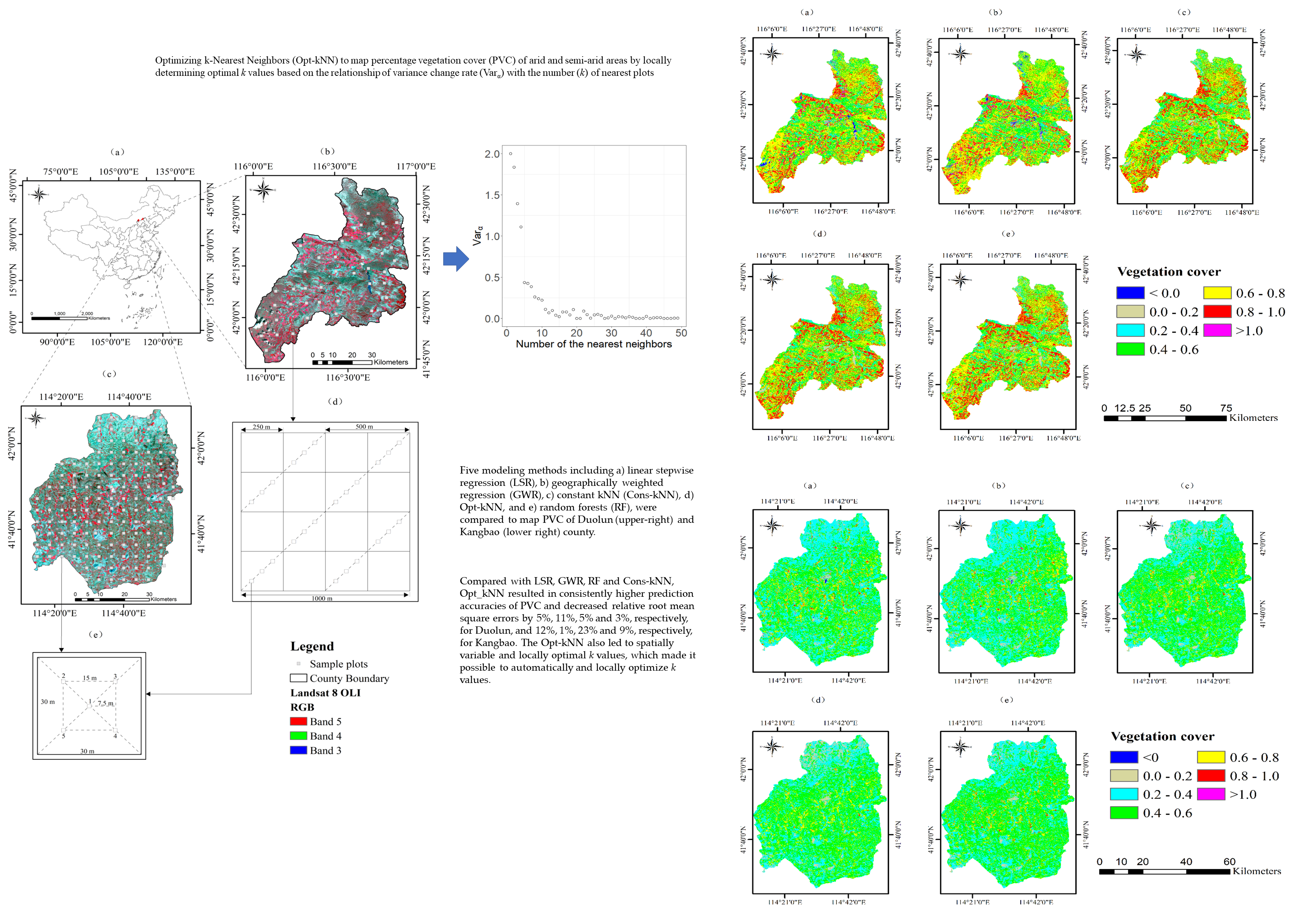
Based on the methodological framework of this study (Figure 1), field data of PVC and remote sensing images were first collected, and various spectral variables were derived from the images. The spectral variables were then selected using correlation analysis and LSR with a variance inflation factor (VIF) to obtain a set of the spectral variables that statistically had significant contributions to improving the mapping of PVC and were not correlated with each other. Moreover, the Cons_kNN algorithm was optimized to find spatially variable and optimal k values that were needed to generate accurate predictions of PVC, which led to the optimized kNN (Opt_kNN). The Opt_kNN was finally applied to map PVC of these two study areas and the obtained results were validated by comparing with other four widely used methods based on the error assessment between field observations and predictions of PVC.
2.1. Study Areas
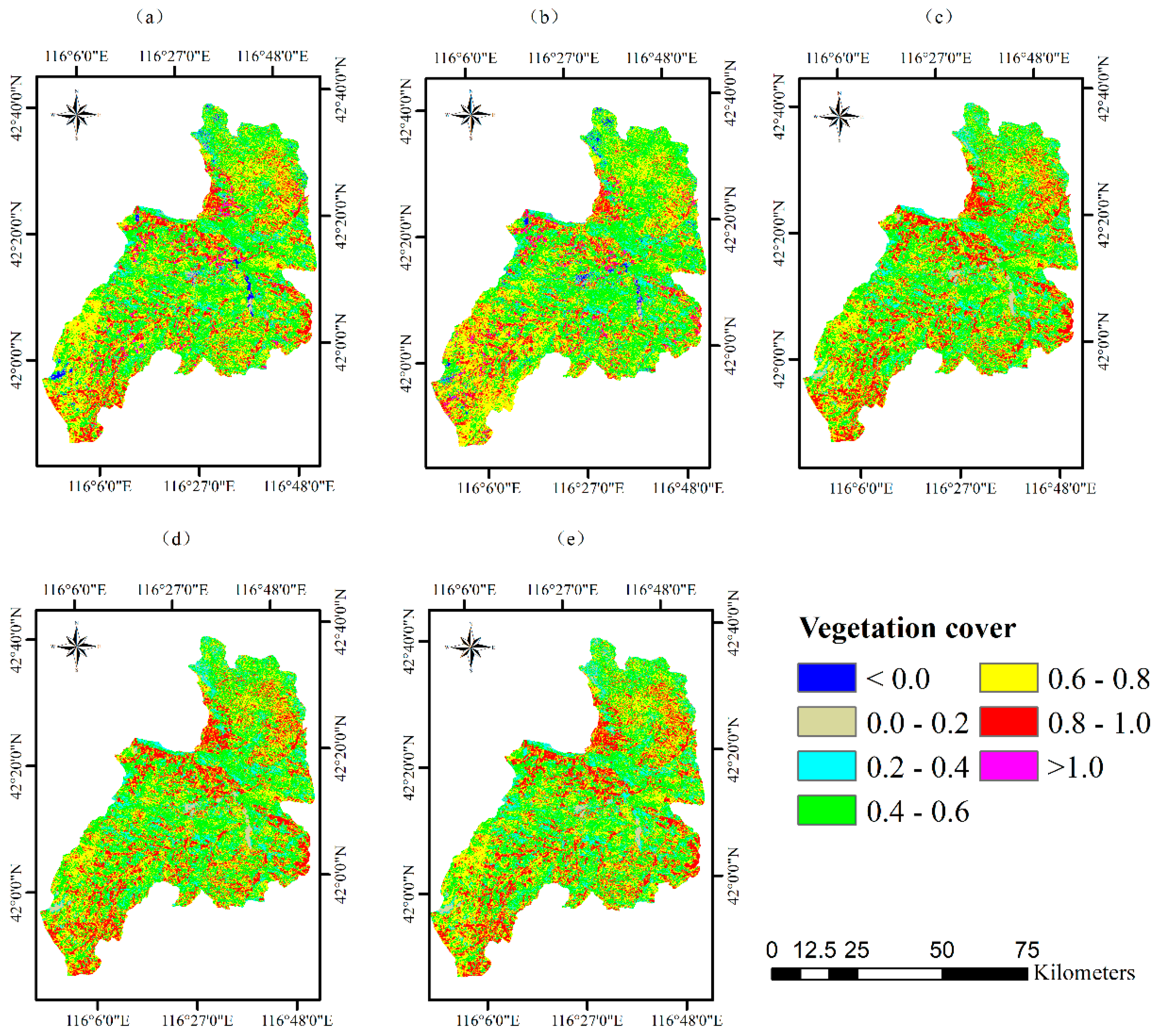
Duolun and Kangbao County were located in the southeast of Xilingol League, Inner Mongolia, and northwest Hebei in Northern China, respectively (Figure 2a). Duolun County has a total area of 3863 km2 and lies within the ranges of latitudes and longitudes from 41°46′ to 42°36′ N and from 115°51′ to 116°54′ E, respectively (Figure 2b). There is 110 km from the north to the south and 70 km from the east to the west. Duolun borders Hexigten Banner to the north, Fengning County and Guyuan County to the south, Plain Blue Banner to the west, and Weichang County to the east. Duolun County has a dry and monsoon-influenced humid continental climate. Its annual average temperature and precipitation were 1.6 °C and 385 mm, respectively. Duolun County was characterized by a typical farming and pastoral zone with a variety of land use and cover types, including croplands, grasslands, shrubs, forests, urbanized areas, water bodies, and bare and sandy areas. It is also involved in a national key ecological construction project. The PVC increased from 0.3 in 2000 to about 0.6 in 2016 since the implementation of Beijing and Tianjin sandstorm source control project proposed by the State Forestry Administration in 2002. As shown in a false color composite image from the combination of Landsat 8 operational land imager (OLI) band 5, band 4, and band 3, bare and sandy areas (cyan in Figure 2b) dominated the north part and scattered mainly in the central area. Vegetated areas (red in Figure 2b) were distributed in the northwest, west, southwest, south, southeast, and east parts.
Kangbao County has an area of 3365 km2 with an average elevation of 1450 m decreasing from the northeast to the southwest. It neighbors Inner Mongolia in the north and has a distance of 350 km to Beijing city in the south (Figure 2a). Its annual average temperature and precipitation were 2.1 °C and 350 mm, respectively. As shown in the false color composite image, bare and sandy areas (cyan in Figure 2c) dominated the north parts and scattered in other parts of the county. Vegetated areas (grasslands, shrubs, croplands, and forests (red in Figure 2c) were mainly distributed in the middle parts from the east to the west and scattered in the south. Although the percentage forest cover of this county had been increasing since the implementation of the Beijing and Tianjin sandstorm source control project in 2002, the overall PVC was about 0.43 and much lower than that of Duolun County.
2.2. Sampling Design and Collection of PVC Field Observations
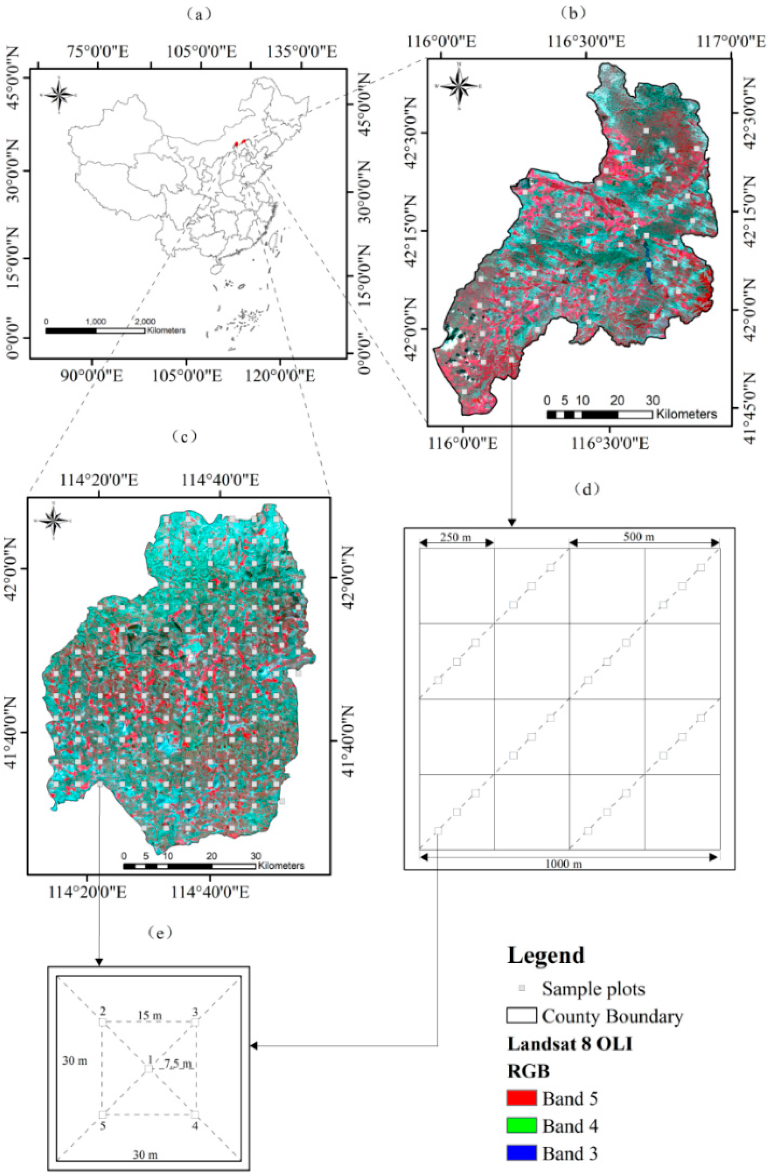
A stratified systematic sampling method was conducted in Duolun County. This county was first divided into 1000 m × 1000 m blocks and 60 sample blocks were systematically selected with a distance interval of 8 km (Figure 2b). Based on a NDVI map generated using Landsat 8 OLI images acquired in August of 2015, the NDVI values were grouped into five classes with an interval of 0.2. The area of each class was derived and the number of the sample blocks for each class was determined proportionally based on the area of the corresponding class. Then, some of the blocks were randomly removed and some of them were modified by slightly shifting their locations. Finally, a total of 40 sample blocks were obtained for this study area (Figure 2b). Each of the sample blocks was further divided into sub-blocks of 250 m × 250 m and 500 m × 500 m. A total of six 30 m × 30 m sample plots were allocated along the diagonal line from the northeast to the southwest within each 500 m × 500 m sub-block and the sampling distance among three sample plots was equal within the 250 m × 250 m sub-blocks. Thus, a total of 24 sample plots were measured within each of the 1000 m × 1000 m sample blocks (Figure 2d). There were five 1 m × 1 m sub-plots allocated within each of the 30 m × 30 m sample plots, and one was located in the plot center and other four located in the diagonal lines (Figure 2e). All the five sub-plots were spatially configured so that to obtain a sampling distance of 15 m between them.
A Trimble Geo 7X global positioning system (GPS) receiver was used for navigation and collection of the plots center coordinates. At the same time, a compass and a tape were adopted to locate four other sup-plots. The PVC values were recorded at an interval of 10 cm along the west-east and north-south central lines within each of the 1 m × 1 m sub-plots. The number of the points covered by vegetation was divided by the total of the observed points, which led to the PVC value of one central line. The average value of two central lines was treated as the PVC value of the sub-plot. Similarly, the mean value of five sub-plots was used as the PVC value of the 30 m × 30 m plot. A total of 960 30 m × 30 m field plots were investigated from 13 July 2016 to 20 August 2016. The plots fell in nine land use and cover types, including cropland, crop & grass mixed land, grassland, grass & shrub mixed land, forest, grass and forest mixed land, urbanized area, water body, and bare and sandy area. There were 40 sample plots involved in one and half 1000 m × 1000 m blocks and covered by clouds, and thus removed from the data analysis. Finally, a total of 920 sample plots were available for Duolun. The plots had larger values of PVC in the southwest and northeast parts than other parts of Duolun County (Figure 3a).
In Kangbao County, a total of 134 30 m × 30 m field plots with a sampling distance of 5 km were systematically sampled and measured from 16 July to 7 August 2014 (Figure 2c). Within each of the plots, five 1 m × 1 m sub-plots were allocated, and their PVC values were collected in the same way as done in Duolun County (Figure 2e). The PVC values of the plots were smaller in the north part of Kangbao County and larger in the central part from the west to the east (Figure 3b). But, overall, Kangbao had a smaller PVC mean value than Duolun.
2.3. Landsat 8 Images and Enhancement
Landsat 8 OLI images dated on 8 August 2016 (Path 123, Row 031) and 15 August 2016 (Path 124, Row 031) were acquired for Duolun County from website: http://glovis.usgs.gov/, and both dates fell in the time interval during which the field survey was conducted. The 8 August image covered more than 90% of Duolun’s area, and the 15 August image occupied less than 10% at the southwest corner. The spatial resolution (30 m × 30 m) of Landsat 8 band 2 to band 7 including blue, green, red, near infrared, shortwave near infrared bands 1 and 2 was consistent with that of the plots. The Landsat OLI data were preprocessed to eliminate the influence of aerosol in the atmosphere and improve the image quality. The pixel values of the two images were first converted to radiance and then to spectral reflectance values after radiation calibration using the atmospheric and topographic correction (ATCOR) model of ERDAS IMAGINE 2013. After that, solar elevation angle correction and Minnaert correction were executed owing to the different image acquisition dates. Moreover, although Landsat L1T products have been already orthorectified, it was found that compared with the coordinates of road intersections obtained using the aforementioned GPS, the image coordinates of the same locations had positional errors larger than 15 m. Thus, geometric corrections were carried out using a second-order polynomial model and 28 ground control points collected with the same GPS. The root mean square error (RMSE) between the coordinates of the ground control points and the coordinates of the same locations on the corrected image was less than 0.5 pixels (15 m).
In order to improve the correlations of PVC with spectral variables, in this study a total of 248 spectral variables were derived from the Landsat 8 images of Duolun County. The spectral variables included seven original OLI bands, NDVI, ARVI, EVI, MNDVI, red-green vegetation index (RGVI), reduced simple ratio (RSR), triangular vegetation index (TVI), visible atmospherically resistant index (VARI), four SAVIi indices (i = 0.1, 0.25, 0.3 and 0.5) [63], 42 two-band difference indices, 42 two-band ratio indices, 105 three-band ratio indices [64], and 40 similar normalized difference vegetation indices (Table 1). The similar normalized difference vegetation indices were derived using the Landsat 8 visible bands, near infrared band and shortwave near infrared bands in the same way as NDVI, but NDVI and RGVI were excluded. Pearson product moment correlation coefficients of the spectral variables with the plot PVC values were calculated to select the spectral variables that were significantly correlated with the PVC at the significance level of 0.05. After that, collinear diagnosis among these significant variables was conducted using LSR with a variance inflation factor (VIF). The finally selected variables were utilized to develop prediction models of PVC.
A Landsat 8 OLI image dated on 1 August 2014 was also downloaded and used for Kangbao County. As conducted for Duolun County, the same methods for image pre-processing, extraction, and selection of spectral variables (Table 1) were utilized for Kangbao County.
2.4. Optimizing K-Nearest Neighbors
In Cons_kNN, a spectral distance for an estimated pixel, p, to each of the sample plots, is first calculated as follows:
where i is a pixel collocated with a plot i, represents the spectral distance between the estimated pixel p and the pixel corresponding to the ith plot, j represents the jth spectral variable, m is the number of the spectral variables, represents the value of the spectral variable j for pixel p, and is the value of the spectral variable j for plot i. The spectral distances are then used to rank the sample plots and the k nearest plots are selected. The estimate of PVC for pixel p is finally obtained by weighting the values of PVC from the k nearest plots with the inverse values of their distances,
where is the PVC value of pixel p, and is the PVC estimate of pixel p.
In order to improve Cons_kNN, in this study a novel method used to locally optimize the k values was proposed. In the proposed method, it is assumed that at each location there is an optimal k value that can lead to the most accurate estimate of PVC for this location. Moreover, the optimal k value spatially varies and differs from place to place due to the spatial variability of PVC. At an unobserved location, the optimal k value is unknown. Given a k value, however, the k nearest plots for an unobserved location can be determined based on the rank of the spectral distances calculated using Equation (1). An estimate for the unobserved location can be then derived by weighting the PVC values of the k nearest plots using Equation (2). The estimate is a weighted mean and denoted with . The uncertainty of the estimate can be indirectly measured using, , the variance of the estimate and calculated as follows:
Changing the value of k results in a corresponding variance. Then, the variance change rate of the PVC estimates for an estimated pixel p between the previous and current k values is
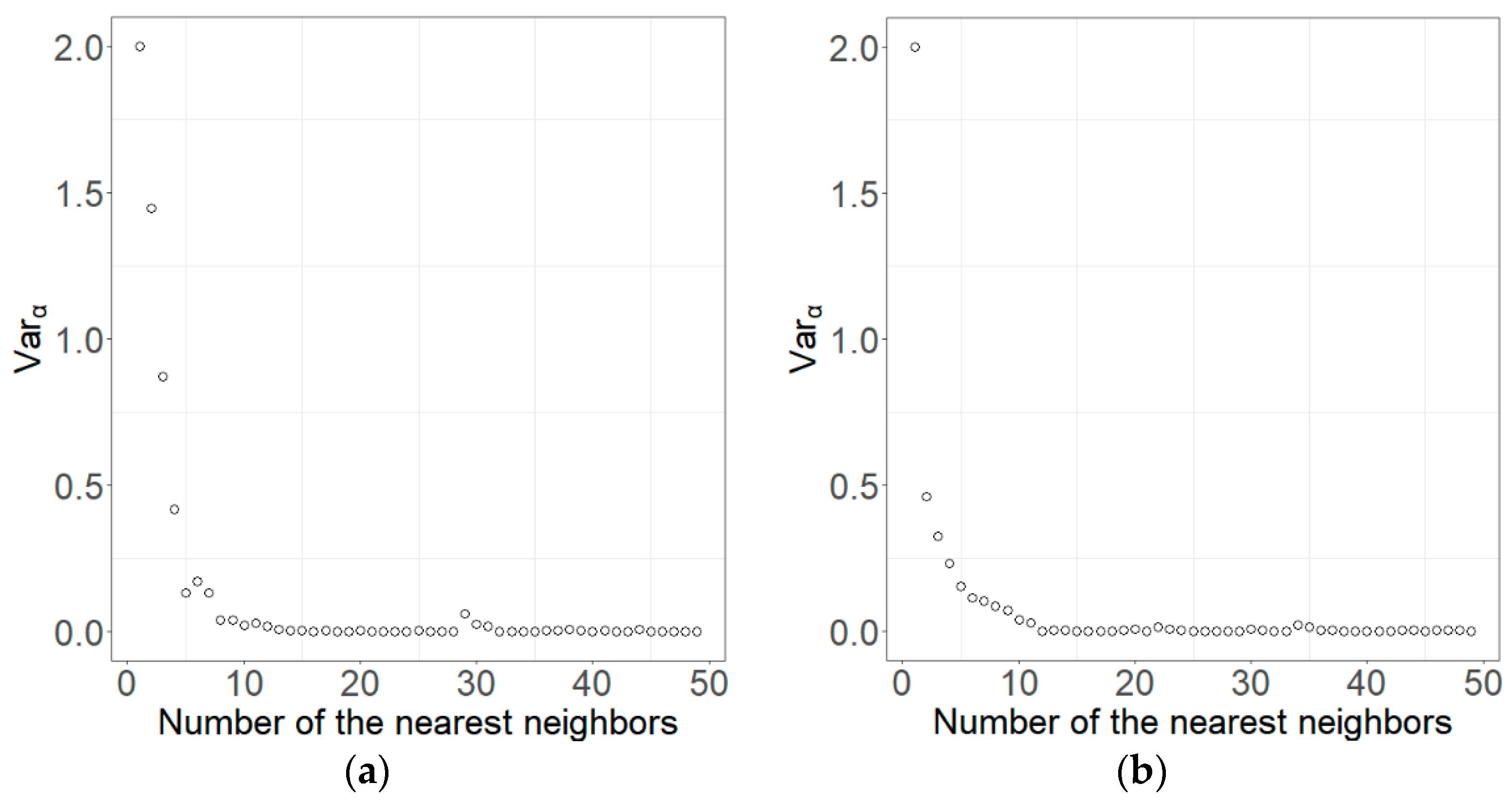
Graphing the values of the variance change rate against the values of k can lead to the relationship of the variance change rate with the number of nearest plots. Theoretically, as the k value increases, the variance change rate decreases rapidly at the beginning, then slowly and gradually gets stable. The optimal k value should be the one that corresponds to the variance change rate that starts to become stable. The relationship varies from place to place, implying that if the relationship is derived for each location, the optimal k value for each location of a study area can be found. Thus, the optimal k values obtained from the relationships would vary spatially.
As examples, Figure 4 showed the relationships for two randomly selected pixels to be estimated for Duolun County. As the k value increased, the variance change rate quickly decreased at the beginning, then slowly and eventually became stable. We also randomly selected two pixels to be estimated in Kangbao and generated the relationship of variance change rates () against k values (Figure 5). The relationships of these two pixels obtained in Kangbao were similar to those derived in Duolun. For any location of a study area, if the relationship is obtained, an optimal k value can be found.
We programmed the improved method Opt_kNN and found an optimal k value for each pixel of 30 m × 30 m in both Duolun and Kangbao County. Using the k values, we generated the spatial distributions or maps of PVC for both study areas. We then assessed the accuracy of the maps and compared the results with those from LSR, GWR, Cons_kNN and RF in both Duolun and Kangbao County. To validate the improvement of the PVC estimation accuracy obtained by Opt_kNN, Cons_kNN with a global optimal constant k value was selected for comparison. Moreover, LSR was chosen because it is a most widely used spatial interpolation method and models the global relationship of PVC with the spectral variables that significantly contributed the reduction of estimation errors. GWR generates the local relationship of PVC with the spectral variables and leads to spatially variable regression coefficients. Compared with the global method LSR, GWR provides the potential to improve the estimation of PVC due to the local modeling of the relationship.
In addition, as a machine learning algorithm, RF has become very popular during the past few years due to its good performance in both classification of categorical variables and prediction of continuous variables [65,66,67,68,69,70,71,72,73]. As done in classification, RF generates a large number of sub-sample data sets by randomly selecting sample plots from the entire sample plot data set with replacement and each of the sub-sample data sets leads to a regression tree that can be used to develop a prediction model. All the models that are independent with each other are utilized to make predictions and averaging the predictions from all the models for each location results in the final estimate of PVC. This mechanism provides the potential to obtain accurate predictions. RF also has the ability of optimizing selection of spectral variables by calculating the mean decrease in accuracy before and after a spectral variable is permuted. Thus, RF can optimize both the selection of spectral variables and the estimation of a dependent variable. In this study, we also tested the sensitivity of the number of the used regression trees (ntree) based on the rate of out-of-bag (OOB) error.
2.5. Evaluation and Comparison of Predictions
In Duolun County, a total of 920 sample plots were randomly separated into two parts: 600 plots and 320 plots. The 600 plots were employed to map PVC using the methods and the 320 plots were utilized to assess the accuracy of the predicted PVC values by comparing the predicted values with the field observations or referenced values. In Kangbao County, there were only 134 sample plots available, and thus a leave-one-out cross validation was utilized for the accuracy assessment and comparison of the methods. The measures used to quantify the accuracy of the predictions included coefficient of determination (R2), mean PVC predictions (MPVC), relative bias (RBias), RMSE and relative RMSE (RRMSE) for the test plots, and coefficient of variation (), mean value (), and variance of the prediction maps () [34,58]. Because the field observations of PVC for the plots were obtained by averaging the values of five 1 m × 1 m subplots within each of the 30 m × 30 m plots, the field observations contained uncertainties and were thus regarded as referenced values.
3. Results
3.1. Statistics of Sample Plot Data
In Duolun County, the values of PVC for all the plots had a sample mean of 0.615 (Table 2). The sample standard deviation and coefficient of variation were 0.246 and 40%, respectively. The modeling dataset had a slightly larger mean, standard deviation and coefficient of variation than the test dataset and the whole dataset. However, statistically there were no significant differences of the mean values among the three datasets at the significant level of 0.05. The confidence intervals for all the plots, the modeling and test datasets were from 0.60 to 0.63, from 0.60 to 0.64, and from 0.58 to 0.63, respectively.
Kangbao County had an average PVC value of 0.430 (Table 2) with a confidence interval of 0.40 to 0.46 at the significant level of 0.05. Compared with that of Duolun County, the mean PVC of the plots for Kangbao County was much smaller, implying that desertification was more serious in Kangbao.
3.2. Selection of Spectral Variables
In Duolun County, Pearson product moment correlation coefficients of 248 spectral variables with the plot PVC from the modeling dataset of 600 sample plots had a range of −0.853 to 0.828. There were 152 spectral variables that were significantly correlated with the plot PVC at the 0.05 significant level. The absolute values of the correlation coefficients of 98 spectral variables were greater than 0.550. The most correlated ten spectral variables were SR435, SR415, SAVI0.25, SAVI0.3, SR215, SAVI0.1, ARVI, SAVI0.5, SR235, and EVI, and their correlation coefficients were −0.853, −0.844, 0.828, 0.827, −0.827, 0.825, 0.822, 0.821, −0.811, and 0.804, respectively. Four SAVI variables had high correlations with the plot PVC. However, the variables were highly correlated with each other. Thus, it was necessary to carry out a collinearity diagnosis before they were used to develop the prediction models. Seven spectral variables including Band4, ARVI, NDVI52, SR32, SR134, SR547, and SR624 were finally reserved after the collinearity diagnosis with a VIF value of 100. The reserved variables were further executed to generate the estimation models using LSR. Finally, five spectral variables, including Band4, ARVI, NDVI52, SR32, and SR134, were selected to map PVC for Duolun County using all the methods. Correspondingly, the selected spectral variables to map PVC for Kangbao County were ARVI, SR514 and Band 1.
3.3. Comparison of Methods
For Duolun, the modeling dataset was used to map PVC and the test data set was utilized to compare the methods. For Kangbao, the mapping and accuracy assessment of PVC were conducted using the leave-one-out cross validation. The Opt_kNN method led to the spatially variable optimal k values, that is, the different optimal numbers of the nearest plots, used to map PVC for Duolun County (Figure 6a) and Kangbao County (Figure 6b). The optimal k values differed from place to place and varied from 3 to 50. In the water bodies and homogeneous areas, the optimal k values were smaller, while in the areas with large spatial variability of PVC, the optimal k values were greater.
For Cons_kNN, we examined different k values of 3 to 51. The maximum constant k value of 51 for Cons_kNN was used because the local maximum optimal k value from Opt_kNN was 50. With the different k values, Cons_kNN was run to generate the maps of PVC for Duolun and Kangbao County. The accuracies of the estimation maps were then assessed based on the test data set for Duolun County and using the leave-one-out cross validation for Kangbao County.
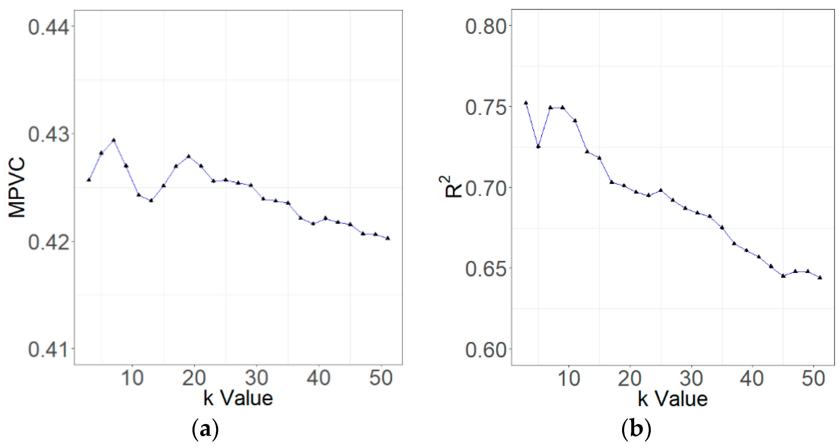
The Con_kNN method with different k values led to the mean predictions of PVC that fell in the confidence interval of the test data for Duolun County and the confidence interval of all the sample plot data for Kangbao County at the significant level of 0.05, although the mean predictions fluctuated (Figure 7a and Figure 8a). For Duolun County, moreover, as the globally constant k value increased, the coefficient of determination R2 increased at the beginning, reached its maximum value when k = 11 and then decreased (Figure 7b). With the increased k values, RRMSE and decreased at the beginning, reached their minimum values when k = 11, and then increased (Figure 7c,d). This indicated that the k = 11 was globally optimal for Duolun. For Kangbao County, R2 had the maximum value when k = 3 and then continuously decreased with the increased k value, except there was an increase of R2 value when the k value increased from 5 to 7 (Figure 8b). With the increased k values, RRMSE and continuously increased. This implied that the globally optimal k value for Kangbao was 3 (Figure 8c,d).
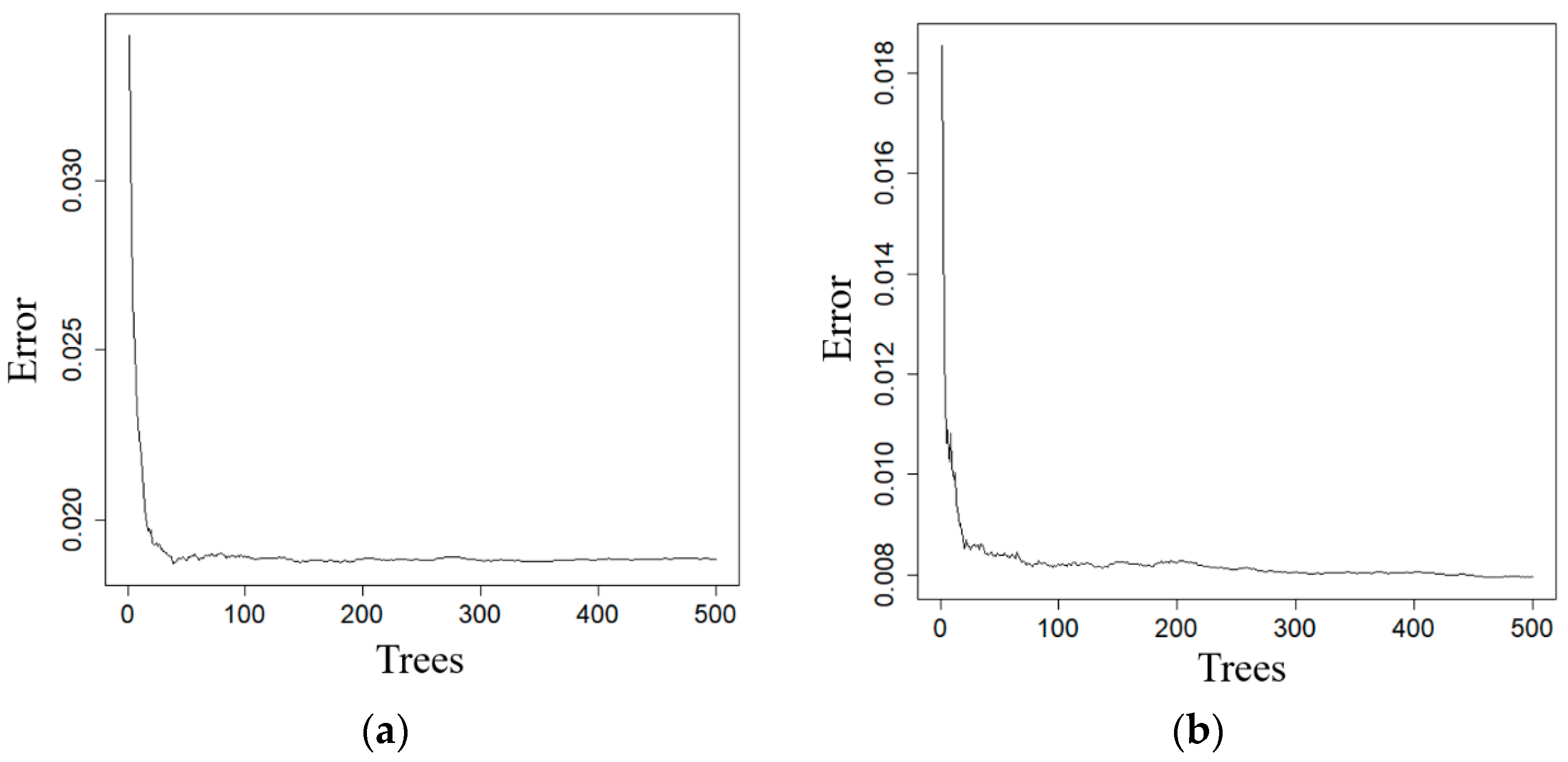
In Figure 9, the estimation error was graphed against the number of the regression trees used in RF for both Duolun and Kangbao County. With the increased number of the regression trees, the error decreased rapidly at the beginning, then slowly and eventually got stable. The 300 and 200 regression trees resulted in the stable error and were thus used for Duolun and Kangbao County, respectively.
In Table 3, the results of predicted PVC using Opt_kNN were compared with those using LSR, GWR, Cons_kNN, and RF for Duolun and Kangbao County. The globally optimal k values were 11 and 3 for Duolun and Kangbao, respectively. For Duolun, there were no statistically significant differences among the coefficients of determination R2 between the referenced and estimated values of PVC from the methods. Similar characteristics were found in Kangbao County, except for RF had a much smaller R2 than the other methods. All the methods led to the plot and map average predictions of PVC that fell in the confidence intervals of the test plot dataset for Duolun County and the whole sample plot dataset by the leave-one-out cross validation for Kangbao County at the significant level of 0.05. Moreover, the values of RBias for the plot predictions of PVC were not significantly different from zero for all the methods.
For Duolun County, Opt_kNN led to the smallest value of RRMSE, then Const_kNN, LSR, RF and GWR. The values of RMSE using the methods Opt_kNN, Const_kNN, RF and LSR statistically did not significantly differ from each other at the significant levels of 0.05 and 0.10. However, the value of RMSE from GWR was statistically significantly larger than that using Opt_kNN at the significant level of 0.05 and using Cons_kNN at the significant level of 0.10. For Kangbao County, Opt_kNN also resulted in the smallest RRMSE value, then GWR, Cons_kNN, LSR and RF. The RMSE value of RF was statistically significantly larger than those from Opt_kNN and GWR at the significant level of 0.05. Overall, Opt_kNN had the highest prediction accuracy for both Duolun and Kangbao County, while the lowest estimation accuracy was obtained using GWR for Duolun and RF for Kangbao. In addition, RF also led to the secondly largest RMSE value for Duolun.
For Duolun County, the spatial distributions of the predicted PVC values using all the methods looked very similar to each other (Figure 10) and they were also similar with that of the plot PVC referenced values in Figure 3a. The southwest and northwest parts had larger PVC prediction values than other parts. The exception was that LSR and GWR led to the negative prediction values and those larger than 1.0 at some places located in the eastern central, west and southwest parts of the study area. The similar spatial patterns of the predicted PVC values from all the methods, and the aforementioned shortcomings of LSR and GWR were also found in the prediction maps of PVC for Kangbao County (Figure 11). Moreover, in Kangbao the smaller PVC prediction values dominated the north parts and the larger estimates were mainly distributed in the central areas.
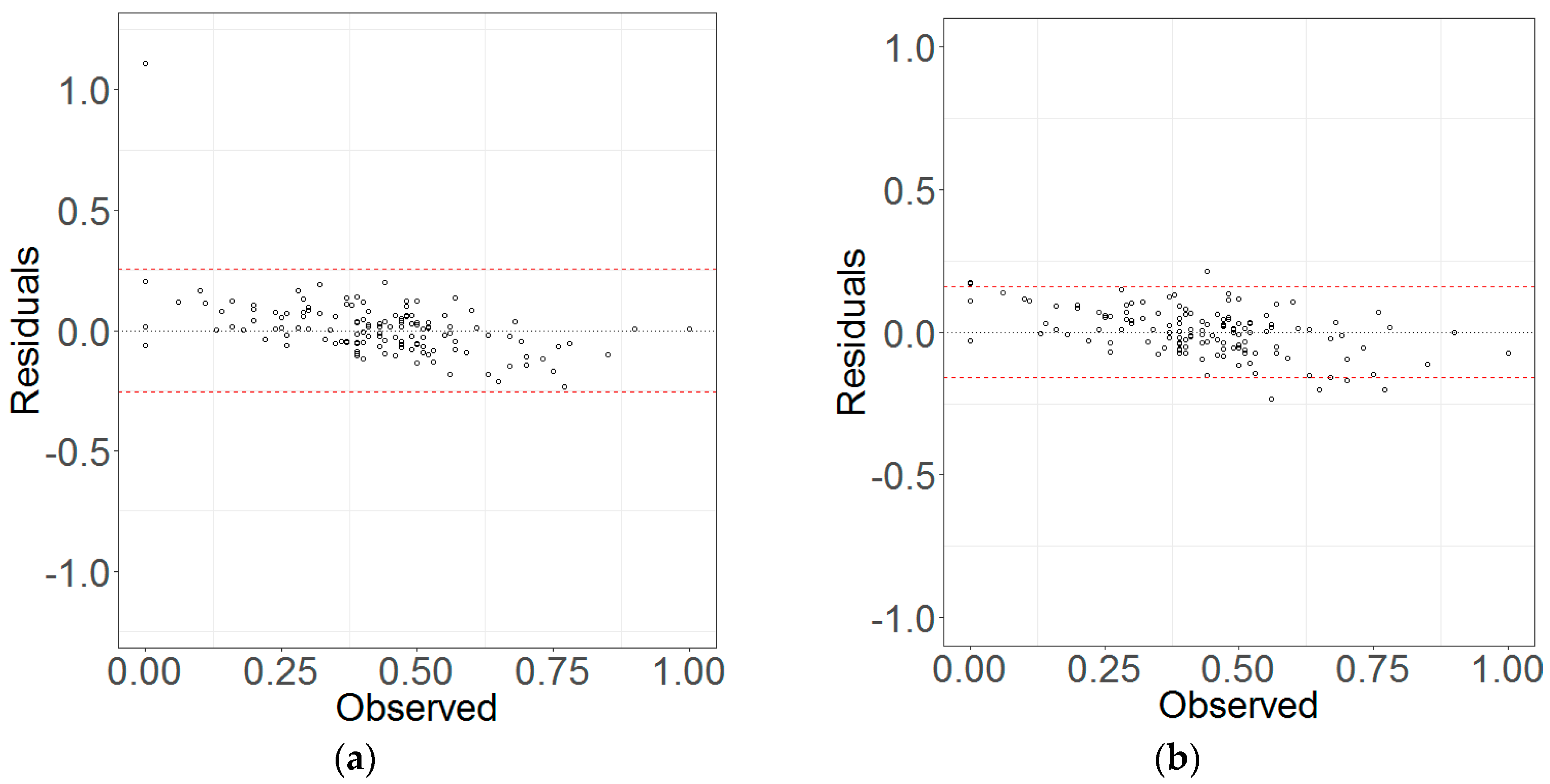
In Figure 12 and Figure 13, the residuals of the PVC predictions were graphed against their referenced values for Duolun and Kangbao County, respectively, using the methods. For both Duolun and Kangbao County, all the methods did not lead to obvious overestimations and underestimations of PVC for the smaller and larger values, respectively, and most of the residuals fell into their confidence intervals of zero. However, Opt_kNN resulted in relatively smaller maximum values of the residuals for both study areas. For Kangbao County (Figure 13), Opt_kNN, LSR and GWR produced similar distributions of the residuals with only slight overestimations and underestimations for the smaller and larger values, respectively. That is, only few of the residuals were out of their confidence intervals of zero. But, the overestimations and underestimations were more obviously noticed in the relationship of the residuals with the referenced values of the plot PVC when Cons_kNN and RF were used (Figure 13c,e). In addition, LSR created an extremely large and positive residual (Figure 13a).
4. Discussion
4.1. Optimized kNN
Cons_kNN is a simple and local spatial interpolation technique. To estimate the value of a dependent variable at each unobserved location, it searches for and uses k most similar plots in a space consisting of predictor variables instead of a geographic space [51]. Cons_kNN has been widely utilized in many areas, especially in estimation and mapping of forest parameters and classification of land use and land cover types. But, there have been no reports to use Cons_kNN to map PVC. Moreover, the accuracy of results from Cons_kNN is mainly influenced by the number of nearest plots used, distance metric, weighting function, and feature weighting parameters. Several authors have studied the effects of the factors for improving the performance of Cons_kNN (i.e., [57,58,74]). There have also been several reports that deal with determining a globally optimal number of nearest plots, that is, k value. As the k value increases, generally, this method tends to be a global estimation. This is supported by the studies of Tokola et al. [59] and Katila et al. [56], in which they found that as the number of nearest neighbors increased, both the RMSE of estimates and the standard deviation of the mean estimate decreased, and the mean estimate also became closer to the sample mean. Alimjan et al. [62] further improved kNN by combining it with SVM to overcome the problem of optimizing the globally k value. But, their method can be only used for classification of categorical variables and not for estimation of continuous variables. Moreover, because of spatial variability of an estimated variable, the optimal k value may differ from place to place. To date, there have been no effective methods used to determine the locally optimal k values. In this study, we proposed a novel method, Opt_kNN, based on the relationship of variance change rate with the k value, to locally optimize the k values. We examined the proposed method by mapping PVC using sample plot data and Landsat 8 images in Duolun and Kangbao County.
The results showed that Opt_kNN created spatially variable and optimal k values and led to more accurate predictions of PVC than Cons_kNN in both Duolun and Kangbao County. All the plot and map average values of PVC predictions statistically did not significantly differ from the sample means, and the values of relative bias were statistically close to zero. The previous studies of using Cons_kNN focused on mapping forest parameters such as forest height, diameter at breast height and biomass, and the reported RRMSE values usually varied from 15% to 40% [34,45,46,47,51,52,53,54,55,56,59]. In this study, for Duolun and Kangbao, the obtained RRMSE values of predicting PVC were respectively 20.9% and 20.6% when Cons_kNN was utilized, and 20.3% and 18.7% when Opt_kNN was used. Compared with those in the previous studies related to map forest parameters, overall the RRMSE values of this study were smaller. The main reason may be because forest canopies are often multiple layers and the saturation of spectral reflectance affects the accuracy of estimating forest parameters. Moreover, both Duolun County and Kangbao are located in arid and semi-arid regions and mainly vegetated by grass, shrubs and crops that have a single layer of canopy. The saturation of spectral reflectance from the canopies may be not serious. In addition, Opt_kNN, that is, the improvement of Cons_kNN, might have also contributed the reduction of the RRMSE values.
In this study, compared with Const_kNN, Opt_kNN decreased the RRMSE values of predicting PVC by 3% and 11% for Duolun and Kangbao, respectively. Although the RMSE values obtained using Opt_kNN were not statistically significantly smaller than those using Const_kNN, Opt_kNN demonstrated the spatially variable and optimal k values and made it possible to automatically and locally optimize the determination of spatially variable k values.
4.2. Comparison with Other Methods
In this study, in addition to the comparison with Cons_kNN, we also compared Opt_kNN with LSR, GWR, and RF for mapping PVC for both Duolun and Kangbao. Based on the values of RRMSE for Duolun, Opt_kNN performed the prediction best, then Cons_kNN, LSR, RF, and GWR. For Kangbao, Opt_kNN also had the smallest RRMSE value, then GWR, Cons_kNN, LSR, and RF. Moreover, compared with the global modeling LSR, the local modeling GWR improved the accuracy of mapping PVC in Kangbao. However, both LSR and GWR led to negative predictions of PVC and the values larger than 1.0 at many places. The other methods Opt_kNN, Const_kNN, and RF overcame the shortcoming of LSR and GWR. This implied that both global and local linear regression methods were not good choices for mapping PVC of the study areas.
Moreover, as a relatively new and recently popular method [72,73], RF resulted in the lowest and second lowest accuracy of estimating PVC for Kangbao and Duolun, respectively. Especially in Kangbao, the estimation accuracy of PVC from RF was statistically significantly lower than that from Opt_kNN. The reasons might be because Kangbao had a smaller number of the sample plots and was more sparsely vegetated than Duolun. This might imply that RF requires a larger number of sample plots than Opt_kNN. In addition, when RF is utilized to map continuous variables, the estimates are generated by averaging predicted values from regression trees obtained by randomly sampling training plots from the whole data set with replacement. This implies smoothing of predicted values. Therefore, Opt_kNN provided the most accurate and reasonable estimates of PVC for both Duolun and Kangbao and offered greater potential to accurately mapping PVC in the arid and semi-arid areas than the other methods.
4.3. Uncertainties of PVC Estimates
The PVC estimates from Opt_kNN are associated with uncertainties. The uncertainties may be caused by the errors from the field observations of PVC, the image data, the image preprocessing and analysis such as atmospheric correction, and the positional errors from the plot locations and the mismatches between the plots and image pixels. Due to a limited space, we only discussed the effects of the uncertainties from the PVC field observations on the estimates. In this study, within each of the 30 m × 30 m sample plots we only measured the PVC values of five 1 m × 1 m square subplots due to a high cost and labor intensity and used their average as the PVC value of the plot. Thus, the average values were associated with uncertainties and could be only utilized as the references of the plot PVC values. In Figure 14, we graphed the coefficients of variation (CV) of the PVC observations within the plots against their means for Duolun and Kangbao County. It was noticed that as the PVC values increased, the CV values decreased, implying that the uncertainties decreased with the increased PVC values. That is, in the sparsely vegetated areas the uncertainties were higher than those in the densely vegetated areas. The uncertainties should be investigated in more detail in the future.
Moreover, we collected the PVC field observations from 13 July and 20 August 2016 and acquired the Landsat images on 8 August and 15 August 2016 for Duolun. For Kangbao, the corresponding dates for the field data collection and the image acquisition were from 16 July to 7 August 2014 and 1 August 2014, respectively. Thus, there were time gaps between the dates of collecting the field data and taking the images for both study areas. The time gaps inevitably existed because the field survey could not be completed within the same day on which the images were acquired. However, the vegetation especially crop growing during the time gaps would cause uncertainties of the PVC estimates. We investigated the uncertainties by graphing the residuals of the plot PVC estimates from Opt_kNN against the time gaps in Figure 15. The time gaps were represented using negative numbers if the field survey was conducted before the image acquisition and otherwise using positive numbers. It was found that the residuals of the predictions from Opt_kNN randomly fell at both sides of the zero-residual line as the time gaps changed from zero, the same day for obtaining the field data and the images, to the negative time gaps, implying the field data were collected before the image acquisition, and the positive time gaps, implying the field data were collected after the image acquisition. There were no obviously systematical biases. Thus, the effects of the uncertainties on the PVC estimates due to the time gaps between the dates of collecting the field data and taking the images could be ignored.
5. Conclusions
Accurately mapping PVC of arid and semi-arid areas is critical for regional and global land degradation and desertification evaluation. The traditional methods such as regression modeling often cannot provide accurate predictions of PVC in the areas. The nonparametric Cons_kNN is a good alternative. However, the use of a globally constant k value in Cons_kNN limits its increasing prediction accuracy due to the spatial variability of PVC in the areas. In this study, an optimized kNN method, Opt_kNN, was proposed and used to map PVC of both Duolun and Kangbao County located in Inner Mongolia and Hebei Province of China using Landsat 8 images and sample plot data. The Opt_kNN was compared with Cons_kNN, LSR, GWR and RF to improve the mapping of PVC for these two study areas. The results showed that (1) most of the red and near infrared band relevant vegetation indices had significant contributions to improving the accuracy of mapping PVC in the study areas; (2) compared with LSR, GWR, RF, and Cons_kNN, Opt_kNN resulted in consistently higher prediction accuracies of PVC and decreased the RRMSE values by 5%, 11%, 5%, and 3%, respectively, for Duolun, and 12%, 1%, 23%, and 9%, respectively, for Kangbao—the Opt_kNN also output spatially variable and locally optimal k values, which made it possible to automatically and locally optimize k values; and (3) the RF method did not perform the performance better than the Opt_kNN for the both areas. Thus, the proposed method is very promising to improve mapping PVC in the arid and semi-arid areas.
Author Contributions
H.S., Q.W. and G. designed the conceptualization and method of this study; X.X., L.R. and H.S. collected the field data and images; H.S. completed the calculation and analysis, and the original draft; G.W. secured the funding, provided the supervision, wrote and revised the manuscript; H.L., P.L., J.L., and S.Z. completed the validation and provided suggestions for analysis.
Funding
This research was funded by the National Bureau to Combat Desertification, State Forestry Administration of China (101-9899), the Fellowship from the China Scholarship Council (201608430021), Hunan Province Science and Technology Plan Project (2015RS4048, 2016SK2026), the China Postdoctoral Science Foundation Project (2014M562147), and Central South University of Forestry and Technology (101-0990).
Conflicts of Interest
The authors declare no conflict of interest.
References
- Veron, S.R.; Paruelo, J.M.; Oesterheld, M. Assessing desertification. J. Arid Environ. 2006, 66, 751–763. [Google Scholar] [CrossRef]
- Reynolds, J.F.; Smith, D.M.S.; Lambin, E.F.; Turner, B.L.; Mortimore, M.; Batterbury, S.P.J.; Downing, T.E.; Dowlatabadi, H.; Fernández, R.J.; Herrick, J.E.; et al. Global desertification: building a science for dryland development. Science 2007, 316, 847–851. [Google Scholar] [CrossRef] [PubMed]
- Mariano, D.A.; dos Santos, C.A.C.; Wardlow, B.D.; Anderson, M.C.; Schiltmeyer, A.C.; Tadesse, T.; Svoboda, M.D. Use of remote sensing indicators to assess effects of drought and human induced land degradation on ecosystem health in Northeastern Brazil. Remote Sens. Environ. 2018, 213, 129–143. [Google Scholar] [CrossRef]
- Dymond, J.R.; Stephens, P.R.; Newsome, P.F.; Wilde, R.H. Percentage percentage vegetation cover of a degrading rangeland from SPOT. Int. J. Remote Sens. 1992, 13, 1999–2007. [Google Scholar] [CrossRef]
- Eklundh, L.; Olsson, L. Vegetation index trends for the African Sahel in 1982–1999. Geophys. Res. Lett. 2003, 30, 1430–1434. [Google Scholar] [CrossRef]
- Schucknecht, A.; Erasmi, S.; Niemeyer, I.; Matschullat, J. Assessing vegetation variability and trends in north-eastern Brazil using AVHRR and MODIS NDVI time series. Eur. J. Remote Sens. 2013, 46, 40–59. [Google Scholar] [CrossRef]
- Lehnert, L.W.; Meyer, H.; Wang, Y.; Miehe, G.; Thies, B.; Reudenbach, C.; Bendix, J. Retrieval of grassland plant coverage on the Tibetan Plateau based on a multi-scale, multi-sensor and multi-method approach. Remote Sens. Environ. 2015, 164, 197–207. [Google Scholar] [CrossRef]
- Symeonakis, E.; Drake, N. Monitoring desertification and land degradation over sub-Saharan Africa. Int. J. Remote Sens. 2004, 25, 573–592. [Google Scholar] [CrossRef]
- Wessels, K.J.; Prince, S.D.; Malherbe, J.; Small, J.; Frost, P.E.; VanZyl, D. Can human-induced land degradation be distinguished from the effects of rainfall variability? A case study in South Africa. J. Arid Environ. 2007, 68, 271–297. [Google Scholar] [CrossRef]
- Tchuenté, A.T.K.; De Jong, S.M.; Roujean, J.L.; Favier, C.; Mering, C. Ecosystem mapping at the African continent scale using a hybrid clustering approach based on 1-km resolution multi-annual data from SPOT/VEGETATION. Remote Sens. Environ. 2011, 115, 452–464. [Google Scholar] [CrossRef]
- Boschetti, M.; Nutini, F.; Brivio, P.A.; Bartholomé, E.; Stroppiana, D.; Hoscilo, A. Identification of environmental anomaly hot spots in West Africa from time series of NDVI and rainfall. ISPRS J. Photogramm. Remote Sens. 2013, 78, 26–40. [Google Scholar] [CrossRef]
- Landmann, T.; Dubovyk, O. Spatial analysis of human-induced vegetation productivity decline over eastern Africa using a decade (2001–2011) of medium resolution MODIS time-series data. Int. J. Appl. Earth Obs. Geoinf. 2014, 33, 76–82. [Google Scholar] [CrossRef]
- Chen, Y.; Gillieson, D. Evaluation of Landsat TM vegetation indices for estimating percentage vegetation cover on semi-arid rangelands: a case study from Australia. Can. J. Remote Sens. 2009, 35, 435–446. [Google Scholar] [CrossRef]
- Wang, T.; Yan, C.Z.; Song, X.; Xie, J.L. Monitoring recent trends in the area of aeolian desertified land using Landsat images in China’s Xinjiang region. ISPRS J. Photogramm. Remote Sens. 2012, 68, 184–190. [Google Scholar] [CrossRef]
- Jia, K.; Liang, S.; Gu, X.; Baret, F.; Wei, X.; Wang, X.; Yao, Y.; Yang, L.; Li, Y. Fractional percentage vegetation cover estimation algorithm for Chinese GF-1 wide field view data. Remote Sens. Environ. 2016, 177, 184–191. [Google Scholar] [CrossRef]
- Halperin, J.; LeMay, V.; Coops, N.; Verchot, L.; Marshall, P.; Lochhead, K. Canopy cover estimation in miombo woodlands of Zambia: comparison of Landsat 8 OLI versus RapidEye imagery using parametric, nonparametric, and semiparametric methods. Remote Sens. Environ. 2016, 179, 170–182. [Google Scholar] [CrossRef]
- Becker, F.; Choudhury, B.J. Relative sensitivity of normalized difference vegetation index (NDVI) and microwave polarization difference index (MPDI) for vegetation and desertification monitoring. Remote Sens. Environ. 1988, 24, 297–311. [Google Scholar] [CrossRef]
- Carreiras, J.M.; Pereira, J.M.; Pereira, J.S. Estimation of tree canopy cover in evergreen oak woodlands using remote sensing. For. Ecol. Manag. 2006, 223, 45–53. [Google Scholar] [CrossRef]
- Wang, Z.; Xiao, X.; Yan, X. Modeling gross primary production of maize cropland and degraded grassland in northeastern China. Agric. For. Meteorol. 2010, 150, 1160–1167. [Google Scholar] [CrossRef]
- del Barrio, G.; Puigdefabregas, J.; Sanjuan, M.E.; Stellmes, M.; Ruiz, A. Assessment and monitoring of land condition in the Iberian Peninsula, 1989–2000. Remote Sens. Environ. 2010, 114, 1817–1832. [Google Scholar] [CrossRef]
- Lamchin, M.; Lee, J.Y.; Lee, W.K.; Lee, E.J.; Kim, M.; Lim, C.H.; Choi, H.A.; Kim, S.R. Assessment of land cover change and desertification using remote sensing technology in a local region of Mongolia. Adv. Space Res. 2016, 57, 64–77. [Google Scholar] [CrossRef]
- Munson, S.M.; Long, A.L.; Wallace, C.S.; Webb, R.H. Cumulative drought and land-use impacts on perennial vegetation across a North American dryland region. Appl. Veg. Sci. 2016, 19, 430–441. [Google Scholar] [CrossRef]
- Huerta, E.; van der Wal, H. Soil macroinvertebrates’ abundance and diversity in home gardens in Tabasco, Mexico, vary with soil texture, organic matter and percentage vegetation cover. Eur. J. Soil Biol. 2012, 50, 68–75. [Google Scholar] [CrossRef]
- Jakob, S.; Bühler, B.; Gloaguen, R.; Breitkreuz, C.; Eliwa, H.A.; El Gameel, K. Remote sensing based improvement of the geological map of the Neoproterozoic Ras Gharib segment in the Eastern Desert (NE-Egypt) using texture features. J. Afr. Earth Sci. 2015, 111, 138–147. [Google Scholar] [CrossRef]
- Dubovyk, O.; Menz, G.; Conrad, C.; Kan, E.; Machwitz, M.; Khamzina, A. Spatio-temporal analyses of cropland degradation in the irrigated lowlands of Uzbekistan using remote-sensing and logistic regression modeling. Environ. Monit. Assess. 2013, 185, 4775–4790. [Google Scholar] [CrossRef] [PubMed]
- Foody, G.M. Geographical weighting as a further refinement to regression modelling: An example focused on the NDVI–rainfall relationship. Remote Sens. Environ. 2003, 88, 283–293. [Google Scholar] [CrossRef]
- Keshkamat, S.S.; Tsendbazar, N.E.; Zuidgeest, M.H.P.; Shiirev-Adiya, S.; van der Veen, A.; van Maarseveen, M.F.A.M. Understanding transportation-caused rangeland damage in Mongolia. J. Environ. Manag. 2013, 114, 433–444. [Google Scholar] [CrossRef] [PubMed]
- Serra, P.; Pons, X.; Saurí, D. Land-cover and land-use change in a Mediterranean landscape: a spatial analysis of driving forces integrating biophysical and human factors. Appl. Geogr. 2008, 28, 189–209. [Google Scholar] [CrossRef]
- Fleming, A.; Wang, G.; McRoberts, R.E. Comparison of methods toward multi-scale forest carbon mapping and spatial uncertainty analysis: combining national forest inventory plot data and Landsat TM images. Eur. J. For. Res. 2015, 134, 125–137. [Google Scholar] [CrossRef]
- Wang, G.; Oyana, T.; Zhang, M.; Adu-Prah, S.; Zeng, S.; Lin, H.; Se, J. Mapping and spatial uncertainty analysis of forest vegetation carbon by combining national forest inventory data and satellite images. For. Ecol. Manag. 2009, 258, 1275–1283. [Google Scholar] [CrossRef]
- Wang, G.; Zhang, M.; Gertner, G.Z.; Oyana, T.; McRoberts, R.E.; Ge, H. Uncertainties of mapping aboveground forest carbon due to plot locations using national forest inventory plot and remotely sensed data. Scand. J. For. Res. 2011, 26, 360–373. [Google Scholar] [CrossRef]
- Howard, H.R.; Wang, G.; Singer, S.; Singer, A.B. Anderson. Modeling and Prediction of Land Condition for Fort Riley Military Installation. Trans. ASABE 2013, 56, 643–652. [Google Scholar] [CrossRef]
- Zhao, P.; Lu, D.; Wang, G.; Wu, C.; Huang, Y.; Yu, S. Examining Spectral Reflectance Saturation in Landsat Imagery and Corresponding Solutions to Improve Forest Aboveground Biomass Estimation. Remote Sens. 2016, 8, 469. [Google Scholar] [CrossRef]
- Zhu, J.; Huang, Z.; Sun, H.; Wang, G. Mapping Forest Ecosystem Biomass Density for Xiangjiang River Basin by Combining Plot and Remote Sensing Data and Comparing Spatial Extrapolation Methods. Remote Sens. 2017, 9, 241. [Google Scholar] [CrossRef]
- Collado, A.D.; Chuvieco, E.; Camarasa, A. Satellite remote sensing analysis to monitor desertification processes in the crop-rangeland boundary of Argentina. J. Arid Environ. 2002, 52, 121–133. [Google Scholar] [CrossRef]
- Shrestha, D.P.; Margate, D.E.; Van der Meer, F.; Anh, H.V. Analysis and classification of hyperspectral data for mapping land degradation: An application in southern Spain. Int. J. Appl. Earth Obs. Geoinf. 2005, 7, 85–96. [Google Scholar] [CrossRef]
- Sohn, Y.; McCoy, R.M. Mapping desert shrub rangeland using spectral unmixing and modeling spectral mixtures with TM data. Photogramm. Eng. Remote Sens. 1997, 63, 707–716. [Google Scholar]
- Thorp, K.R.; French, A.N.; Rango, A. Effect of image spatial and spectral characteristics on mapping semi-arid rangeland vegetation using multiple endmember spectral mixture analysis (MESMA). Remote Sens. Environ. 2013, 132, 120–130. [Google Scholar] [CrossRef]
- Xiao, J.; Moody, A. A comparison of methods for estimating fractional green percentage vegetation cover within a desert-to-upland transition zone in central New Mexico, USA. Remote Sens. Environ. 2005, 98, 237–250. [Google Scholar] [CrossRef]
- Zhang, X.; Shang, K.; Cen, Y.; Shuai, T.; Sun, Y. Estimating ecological indicators of karst rocky desertification by linear spectral unmixing method. Int. J. Appl. Earth Obs. Geoinf. 2014, 31, 86–94. [Google Scholar] [CrossRef]
- Archibald, S.; Roy, D.P.; WILGEN, V.; Brian, W.; SCHOLES, R.J. What limits fire? An examination of drivers of burnt area in Southern Africa. Glob. Chang. Biol. 2009, 15, 613–630. [Google Scholar] [CrossRef] [Green Version]
- Zaher, M.A.; Senosy, M.M.; Youssef, M.M.; Ehara, S. Thickness variation of the sedimentary cover in the South Western Desert of Egypt as deduced from Bouguer gravity and drill-hole data using neural network method. Earth Planets Space 2009, 61, 659–674. [Google Scholar] [CrossRef] [Green Version]
- Hassan, S.M.; Soliman, O.S.; Mahmoud, A.S. Optimized data input for the support vector machine classifier using ASTER data. Case study: Wadi Atalla area, Eastern Desert, Egypt. Carpath. J. Earth Environ. 2015, 10, 15–26. [Google Scholar]
- Rayegani, B.; Barati, S.; Sohrabi, T.A.; Sonboli, B. Remotely sensed data capacities to assess soil degradation. Egypt. J. Remote Sens. Space Sci. 2016, 19, 207–222. [Google Scholar] [CrossRef]
- McRoberts, R.E.; Nelson, M.D.; Wendt, D.G. Stratified estimation of forest area using satellite imagery, inventory data, and the k-Nearest Neighbors technique. Remote Sens. Environ. 2002, 82, 457–468. [Google Scholar] [CrossRef]
- McRoberts, R.E.; Magnussen, S.; Tomppo, E.O.; Chirici, G. Parametric, bootstrap, and jackknife variance estimators for the k-Nearest Neighbors technique with illustrations using forest inventory and satellite image data. Remote Sens. Environ. 2011, 115, 3165–3174. [Google Scholar] [CrossRef]
- Tomppo, E.; Olsson, H.; Stahl, G.; Nilsson, M.; Hagner, O.; Katila, M. Combining national forest inventory field plots and remote sensing data for forest databases. Remote Sens. Environ. 2008, 112, 1982–1999. [Google Scholar] [CrossRef]
- Thessler, S.; Sesnie, S.; Bendaña, Z.S.R.; Ruokolainen, K.; Tomppo, E.; Finegan, B. Using k-nn and discriminant analyses to classify rain forest types in a Landsat TM image over northern Costa Rica. Remote Sens. Environ. 2008, 112, 2485–2494. [Google Scholar] [CrossRef]
- Tan, K.; Hu, J.; Li, J.; Du, P. A novel semi-supervised hyperspectral image classification approach based on spatial neighborhood information and classifier combination. ISPRS J. Photogramm. Remote Sens. 2015, 105, 19–29. [Google Scholar] [CrossRef]
- Mura, M.; McRoberts, R.E.; Chirici, G.; Marchetti, M. Statistical inference for forest structural diversity indices using airborne laser scanning data and the k-Nearest Neighbors technique. Remote Sens. Environ. 2016, 186, 678–686. [Google Scholar] [CrossRef]
- Franco–Lopez, H.; Ek, A.R.; Bauer, M.E. Estimation and mapping of forest stand density, volume, and cover type using the k-nearest neighbors method. Remote Sens. Environ. 2001, 77, 251–274. [Google Scholar] [CrossRef] [Green Version]
- Labrecque, S.; Fournier, R.A.; Luther, J.E.; Piercey, D. A comparison of four methods to map biomass from Landsat-TM and inventory data in western Newfoundland. For. Ecol. Manag. 2006, 226, 129–144. [Google Scholar] [CrossRef]
- Fuchs, H.; Magdon, P.; Kleinn, C.; Flessa, H. Estimating aboveground carbon in a catchment of the Siberian forest tundra: Combining satellite imagery and field inventory. Remote Sens. Environ. 2009, 113, 518–531. [Google Scholar] [CrossRef]
- Stümer, W.; Kenter, B.; Köhl, M. Spatial interpolation of in situ data by self-organizing map algorithms (neural networks) for the assessment of carbon stocks in European forests. For. Ecol. Manag. 2010, 260, 287–293. [Google Scholar] [CrossRef]
- Tomppo, E.; Halme, M. Using coarse scale forest variables as ancillary information and weighting of variables in k-NN estimation: a genetic algorithm approach. Remote Sens. Environ. 2004, 92, 1–20. [Google Scholar] [CrossRef]
- Katila, M.; Tomppo, E. Selecting estimation parameters for the Finnish multisource National Forest Inventory. Remote Sens. Environ. 2001, 76, 16–32. [Google Scholar] [CrossRef]
- Tomppo, E.O.; Gagliano, C.; De Natale, F.; Katila, M.; McRoberts, R.E. Predicting categorical forest variables using an improved k-Nearest Neighbour estimator and Landsat imagery. Remote Sens. Environ. 2009, 113, 500–517. [Google Scholar] [CrossRef]
- McRoberts, R.E.; Næsset, E.; Gobakken, T. Optimizing the k-Nearest Neighbors technique for estimating forest aboveground biomass using airborne laser scanning data. Remote Sens. Environ. 2015, 163, 13–22. [Google Scholar] [CrossRef]
- Tokola, T.; Pitkänen, J.; Partinen, S.; Muinonen, E. Point accuracy of a non-parametric method in estimation of forest characteristics with different satellite materials. Int. J. Remote Sens. 1996, 17, 2333–2351. [Google Scholar] [CrossRef]
- Hall, P.; Park, B.U.; Samworth, R.J. Choice of neighbor order in nearest-neighbor classification. Ann. Stat. 2008, 36, 2135–2152. [Google Scholar] [CrossRef]
- James, G.; Witten, D.; Hastie, T.; Tibshirani, R. Introduction to Statistical Learning: With Applications in R; Springer: New York, NY, USA, 2017. [Google Scholar]
- Alimjan, G.; Sun, T.; Liang, Y.; Jumahun, H.; Guan, Y. A New Technique for Remote Sensing Image Classification Based on Combinatorial Algorithm of SVM and KNN. Int. J. Pattern Recognit. Artif. Intell. 2018, 32, 1–23. [Google Scholar] [CrossRef]
- Jenson, J.R. Introductory digital image processing: A remote sensing perspective. J. Geocarto Int. 2008, 2, 65. [Google Scholar] [CrossRef]
- Sun, H.; Qie, G.; Wang, G.; Tan, Y.; Li, J.; Peng, Y.; Ma, Z.; Luo, C. Increasing the accuracy of mapping urban forest carbon density by combining spatial modeling and spectral unmixing analysis. Remote Sens. 2015, 7, 15114–15139. [Google Scholar] [CrossRef]
- Breiman, L. Random forests. Mach. Learn. 2001, 45, 5–32. [Google Scholar] [CrossRef]
- Hao, P.; Zhan, Y.; Wang, L.; Niu, Z.; Shakir, M. Feature Selection of Time Series MODIS Data for Early Crop Classification Using Random Forest: A Case Study in Kansas, USA. Remote Sens. 2015, 7, 5347–5369. [Google Scholar] [CrossRef] [Green Version]
- Koreen Millard, K.; Richardson, M. On the Importance of Training Data Sample Selection in Random Forest Image Classification: A Case Study in Peatland Ecosystem Mapping. Remote Sens. 2015, 7, 8489–8515. [Google Scholar] [CrossRef] [Green Version]
- Sharma, R.C.; Tateishi, R.; Hara, K.; Iizuka, K. Production of the Japan 30-m Land Cover Map of 2013–2015 Using a Random Forests-Based Feature Optimization Approach. Remote Sens. 2016, 8, 429. [Google Scholar] [CrossRef]
- Tin Kam, H. Random decision forests. In Proceedings of the 3rd International Conference on Document Analysis and Recognition, Montreal, QC, Canada, 14–16 August 1995; pp. 278–282. [Google Scholar]
- Tin Kam, H. The Random Subspace Method for Constructing Decision Forests. IEEE Trans. Pattern Anal. Mach. Intell. 1998, 20, 832–844. [Google Scholar] [CrossRef]
- Wessels, K.J.; van den Bergh, F.; Roy, D.P.; Salmon, B.P.; Steenkamp, K.C.; MacAlister; Swanepoel, D.; Jewitt, D. Rapid Land Cover Map Updates Using Change Detection and Robust Random Forest Classifiers. Remote Sens. 2016, 8, 888. [Google Scholar] [CrossRef]
- Chen, T.; Trinder, J.C.; Niu, R. Object-Oriented Landslide Mapping Using ZY-3 Satellite Imagery, Random Forest and Mathematical Morphology, for the Three-Gorges Reservoir, China. Remote Sens. 2017, 9, 333. [Google Scholar] [CrossRef]
- de Castro, A.I.; Torres-Sánchez, J.; Peña, J.M.; Jiménez-Brenes, F.M.; Csillik, O.; López-Granados, F. An Automatic Random Forest-OBIA Algorithm for Early Weed Mapping between and within Crop Rows Using UAV Imagery. Remote Sens. 2018, 10, 285. [Google Scholar] [CrossRef]
- Halme, M.; Tomppo, E. Improving the accuracy of multisource forest inventory estimates to reducing plot location error—A multicriteria approach. Remote Sens. Environ. 2001, 78, 321–327. [Google Scholar] [CrossRef]
Figure 1.
Methodological framework of this study.

Figure 2.
(a) Locations of two study areas (Duolun and Kangbao) in China; (b) Duolun County shown using a Landsat operational land imager (OLI) composition image consisting of band 5 (red), band 4 (green), and band 3 (blue) with the spatial distribution of 1000 m × 1000 m sampled blocks (grey); (c) Kangbao County shown using a similar composition image with the spatial distribution of systematically sampled plots of 30 m × 30 m; (d) the spatial distribution of nested 250 m × 250 m and 500 m × 500 m sub-blocks, and 30 m × 30 m sample plots in Duolun; and (e) the allocation of five 1 m × 1 m sub-plots within each 30 m × 30 m sample plot for both Duolun and Kangbao.

Figure 3.
The spatial distribution of plot percentage vegetation cover (PVC) values for (a) Duolun County with (a-1) and (a-2): two examples of spatial distribution of 30 m × 30 m plot PVC values within 1000 m × 1000 m blocks; and (b) Kangbao County.
Figure 3.
The spatial distribution of plot percentage vegetation cover (PVC) values for (a) Duolun County with (a-1) and (a-2): two examples of spatial distribution of 30 m × 30 m plot PVC values within 1000 m × 1000 m blocks; and (b) Kangbao County.

Figure 4.
Variance change rates () against k (the number of nearest plots used) for two randomly selected locations (pixels (a) and (b)) to be estimated in Duolun County.
Figure 4.
Variance change rates () against k (the number of nearest plots used) for two randomly selected locations (pixels (a) and (b)) to be estimated in Duolun County.

Figure 5.
Variance change rates () against k (the number of nearest plots used) for two randomly selected locations (pixels (a) and (b)) to be estimated in Kangbao County.
Figure 5.
Variance change rates () against k (the number of nearest plots used) for two randomly selected locations (pixels (a) and (b)) to be estimated in Kangbao County.

Figure 6.
The spatial distributions of the optimal k (the optimal numbers of the nearest plots used) for predicting PVC at each location of (a) Duolun County and (b) Kangbao County using Opt_kNN.
Figure 6.
The spatial distributions of the optimal k (the optimal numbers of the nearest plots used) for predicting PVC at each location of (a) Duolun County and (b) Kangbao County using Opt_kNN.

Figure 7.
The accuracy assessment results of PVC predictions for Duolun County using Cons_kNN with 25 different k based on the test dataset: (a) mean prediction of plot percentage vegetation cover (MPVC) (confidence interval: 0.58–0.63); (b) coefficient of determination, R2; (c) relative root mean square error (RRMSE); and (d) variance of the predicted PVC values for the maps ().

Figure 8.
The accuracy assessment results of PVC predictions for Kangbao County using Cons_kNN with 25 different k and leave-one-out cross validation based on the whole dataset: (a) mean prediction of plot percentage vegetation cover (MPVC) (confidence interval: 0.40–0.46); (b) coefficient of determination, R2; (c) relative root mean square error (RRMSE); and (d) variance of the predicted PVC values for the maps ().


Figure 9.
The error of estimates against the number of the regression trees used in random forest (RF) for (a) Duolun County and (b) Kangbao County.
Figure 9.
The error of estimates against the number of the regression trees used in random forest (RF) for (a) Duolun County and (b) Kangbao County.

Figure 10.
The spatial distributions of percentage vegetation cover predictions for Duolun County using: (a) Linear regression model (LSR); (b) Geographically weighted regression (GWR); (c) Constant kNN (Cons_kNN) with 11 nearest plots; (d) Optimized kNN (Opt_kNN); and (e) Random forest (RF).
Figure 10.
The spatial distributions of percentage vegetation cover predictions for Duolun County using: (a) Linear regression model (LSR); (b) Geographically weighted regression (GWR); (c) Constant kNN (Cons_kNN) with 11 nearest plots; (d) Optimized kNN (Opt_kNN); and (e) Random forest (RF).

Figure 11.
The spatial distributions of percentage vegetation cover predictions for Kangbao County using: (a) Linear regression model (LSR); (b) Geographically weighted regression (GWR); (c) Constant kNN (Cons_kNN) with 3 nearest plots; (d) Optimized kNN (Opt_kNN); and (e) Random forest (RF).
Figure 11.
The spatial distributions of percentage vegetation cover predictions for Kangbao County using: (a) Linear regression model (LSR); (b) Geographically weighted regression (GWR); (c) Constant kNN (Cons_kNN) with 3 nearest plots; (d) Optimized kNN (Opt_kNN); and (e) Random forest (RF).

Figure 12.
The residuals of percentage vegetation cover predictions graphed against the observations or referenced values for Duolun County using: (a) Linear stepwise regression (LSR); (b) Geographically weighted regression (GWR); (c) Constant kNN (Cons_kNN) with 11 nearest plots; (d) Optimized kNN (Opt_kNN); and (e) Random forest (RF). The red dashed lines represented the confidence interval of zone residuals at the significant level of 0.05.


Figure 13.
The residuals of percentage vegetation cover predictions graphed against the observations or referenced values for Kangbao County using: (a) Linear stepwise regression (LSR); (b) Geographically weighted regression (GWR); (c) Constant kNN (Cons_kNN) with 3 nearest plots; (d) Optimized kNN (Opt_kNN); and (e) Random forest (RF). The red dashed lines represented the confidence interval of zone residuals at the significant level of 0.05.


Figure 14.
The coefficient of variation (CV) of the PVC observations from five 1 m × 1m subplots within each of the plots graphed against their mean for (a) Duolun and (b) Kangbao County.
Figure 14.
The coefficient of variation (CV) of the PVC observations from five 1 m × 1m subplots within each of the plots graphed against their mean for (a) Duolun and (b) Kangbao County.

Figure 15.
The residuals of predictions from Opt_kNN graphed against the time gap of the field survey date from the image acquisition date for (a) Duolun and (b) Kangbao (The time gaps were represented using negative numbers if the field survey was conducted before the image acquisition and otherwise using positive numbers).


Table 1.
Spectral variables (SV) extracted from the Landsat 8 OLI images.
| SV | Definition of SV | No of SV | Reference |
|---|---|---|---|
| Original bandi | band1-coastal aerosol, band2-blue, band3-green (GRN), band4-RED, band5-near infrared (NIR), band6-shortwave infrared band 1 (SWIR1) and band7-shortwave infrared band 2 (SWIR2) | 7 | |
| Simple two-band ratios | , | 42 | [64] |
| Three-band ratios | , | 105 | [64] |
| Difference vegetation indices | , | 42 | [64] |
| Normalized difference vegetation index | 1 | [63] | |
| Modified normalized difference vegetation index | 1 | [63] | |
| Red-green vegetation index | 1 | [63] | |
| Reduced simple ratio | 1 | [63] | |
| Soil adjusted vegetation indices | , l = 0.1, 0.25, 0.3, 0.5 | 4 | [63] |
| Atmospherically resistant vegetation index | 1 | [63] | |
| Enhanced vegetation index | 1 | [63] | |
| Triangular vegetation index | 1 | [63] | |
| Visible atmospherically resistant index | 1 | [63] | |
| Similar normalized difference vegetation indices | , Not including NDVI and RGVI. | 40 |
Table 2.
The statistical summary of sample plot data used for mapping PVC for Duolun and Kangbao County.
Table 2.
The statistical summary of sample plot data used for mapping PVC for Duolun and Kangbao County.
| Sample | N. Plots | Minimum | Maximum | Sample Mean | Standard Deviation | Coefficient of Variation (%) |
|---|---|---|---|---|---|---|
| Duolun County | ||||||
| Total | 920 | 0 | 1.0 | 0.615 | 0.246 | 40.0 |
| Modeling dataset | 600 | 0 | 1.0 | 0.619 | 0.253 | 40.8 |
| Test dataset | 320 | 0 | 1.0 | 0.606 | 0.234 | 38.6 |
| Kangbao County | ||||||
| Total | 134 | 0 | 1.0 | 0.430 | 0.180 | 41.8 |
Table 3.
Comparison of percentage vegetation cover (PVC) prediction accuracies among five methods including linear stepwise regression (LSR), geographically weighted regression (GWR), constant kNN with a globally optimal k (Cons_kNN), optimized kNN with local optimal k values, (Opt_kNN) and random forest (RF) for both Duolun and Kangbao County (R2, RMSE and RRMSE are the coefficient of determination, root mean square error and relative RMSE for plots; MPVC and RBias are the mean prediction and relative bias of PVC for the plots; and are the mean prediction and coefficient of variation of PVC for the maps; and the confidence interval was 0.58 to 0.63 for Duolun and 0.40 to 0.46 for Kangbao).
| Methods | R2 | MPVC | RMSE | RRMSE (%) | RBias (%) | ||
|---|---|---|---|---|---|---|---|
| Duolun County | |||||||
| LSR | 0.703 | 0.60 | 0.129 | 21.28 | −0.40 | 33.91 | 0.62 |
| GWR | 0.667 | 0.60 | 0.138 | 22.74 | −1.21 | 33.13 | 0.62 |
| Cons_kNN (k = 11) | 0.711 | 0.61 | 0.127 | 20.90 | 0.42 | 35.20 | 0.63 |
| Opt_kNN | 0.727 | 0.61 | 0.123 | 20.32 | 0.24 | 35.62 | 0.63 |
| RF | 0.702 | 0.61 | 0.130 | 21.40 | 0.59 | 36.14 | 0.63 |
| Kangbao County | |||||||
| LSR | 0.736 | 0.43 | 0.092 | 21.35 | 0.02 | 36.67 | 0.43 |
| GWR | 0.795 | 0.43 | 0.081 | 18.87 | 0.51 | 36.65 | 0.42 |
| Cons_kNN (k = 3) | 0.759 | 0.44 | 0.088 | 20.56 | 1.24 | 33.85 | 0.43 |
| Opt_kNN | 0.753 | 0.43 | 0.080 | 18.70 | −0.44 | 34.01 | 0.44 |
| RF | 0.661 | 0.43 | 0.104 | 24.27 | 0.14 | 34.66 | 0.44 |
© 2018 by the authors. Licensee MDPI, Basel, Switzerland. This article is an open access article distributed under the terms and conditions of the Creative Commons Attribution (CC BY) license (http://creativecommons.org/licenses/by/4.0/).
Share and Cite
MDPI and ACS Style
Sun, H.; Wang, Q.; Wang, G.; Lin, H.; Luo, P.; Li, J.; Zeng, S.; Xu, X.; Ren, L. Optimizing kNN for Mapping Vegetation Cover of Arid and Semi-Arid Areas Using Landsat Images. Remote Sens. 2018, 10, 1248. https://doi.org/10.3390/rs10081248
AMA Style
Sun H, Wang Q, Wang G, Lin H, Luo P, Li J, Zeng S, Xu X, Ren L. Optimizing kNN for Mapping Vegetation Cover of Arid and Semi-Arid Areas Using Landsat Images. Remote Sensing. 2018; 10(8):1248. https://doi.org/10.3390/rs10081248
Chicago/Turabian StyleSun, Hua, Qing Wang, Guangxing Wang, Hui Lin, Peng Luo, Jiping Li, Siqi Zeng, Xiaoyu Xu, and Lanxiang Ren. 2018. "Optimizing kNN for Mapping Vegetation Cover of Arid and Semi-Arid Areas Using Landsat Images" Remote Sensing 10, no. 8: 1248. https://doi.org/10.3390/rs10081248
Note that from the first issue of 2016, this journal uses article numbers instead of page numbers. See further details here.