Airborne Remote Sensing of the Upper Ocean Turbulence during CASPER-East

Abstract

This study takes on the challenge of resolving upper ocean surface currents with a suite of airborne remote sensing methodologies, simultaneously imaging the ocean surface in visible, infrared, and microwave bands. A series of flights were conducted over an air-sea interaction supersite established 63 km offshore by a large multi-platform CASPER-East experiment. The supersite was equipped with a range of in situ instruments resolving air-sea interface and underwater properties, of which a bottom-mounted acoustic Doppler current profiler was used extensively in this paper for the purposes of airborne current retrieval validation and interpretation. A series of water-tracing dye releases took place in coordination with aircraft overpasses, enabling dye plume velocimetry over 100 m to 10 km spatial scales. Similar scales were resolved by a Multichannel Synthetic Aperture Radar, which resolved a swath of instantaneous surface velocities (wave and current) with 10 m resolution and 5 cm/s accuracy. Details of the skin temperature variability imprinted by the upper ocean turbulence were revealed in 1–14,000 m range of spatial scales by a mid-wave infrared camera. Combined, these methodologies provide a unique insight into the complex spatial structure of the upper ocean turbulence on a previously under-resolved range of spatial scales from meters to kilometers. However, much attention in this paper is dedicated to quantifying and understanding uncertainties and ambiguities associated with these remote sensing methodologies, especially regarding the smallest resolvable turbulent scales and reference depths of retrieved currents.

1. Background

Capabilities for spatial measurements of ocean surface turbulence are highly desirable for a wide variety of needs ranging from basic studies of upper ocean mixing processes to data assimilation into high-resolution coastal and ocean circulation models. On the global scale, presently available observations of the ocean currents are provided by satellite altimeters, which are limited to mesoscales and resolve only the geostrophic component of the surface current. Much anticipated launches of the Surface Water and Ocean Topography (SWOT) and Coastal and Ocean measurement Mission with Precise and Innovative Radar Altimeter (COMPIRA) satellite missions will provide some submesoscale altimetry coverage; however, many smaller scale processes, such as non-geostrophic submesoscale turbulence, frontal instabilities, or Langmuir circulations will remain unresolved. Some of these processes are unresolved even by the dense horizontal resolution of surface currents from shore-based high frequency (HF) radars. In situ observations from research vessels or bottom-mounted Acoustic Current Doppler Profilers (ADCP), on the other hand, are essentially Eulerian point measurements, while surface drifters each provide single Lagrangian trajectory. This leaves a wide range of spatial scales from meters to tens of kilometers largely unresolved in the field, leaving hydrodynamic processes taking place on these scales unknown. The hypothesis pursued in this study is that this range of scales can potentially be resolved with an airborne imaging approach.

Generally, airborne ocean remote sensing can employ any band of the electromagnetic spectrum with either sun reflection, passive radiation, or reflection of an actively emitted signal, serving as a source of the measured signal. The need to interpret and relate measured signal in terms of the upper ocean hydrodynamics; however, significantly narrows down available options. Furthermore, even if an obtained image clearly contains some information about the surface turbulence, establishing a quantitative relationship to usable oceanographic variables is always a challenge. Following is a brief overview of some known techniques in visible, infrared, and microwave bands of the spectrum.

1.1. Visible Light Methods

Away from the coast, the small-scale variability of a signal measured by a common airborne visible band image of the ocean surface is mostly due to specular reflections of the sunlight from various facets of surface waves. While repeated attempts to recover wave amplitude spectrum from such imagery have been mostly unsuccessful, it is certainly possible to detect wave phases as they move across an image. With enough dwell time and spatial resolution over each scene, empirical reconstruction of the surface gravity wave dispersion relationship curve is possible, which relates wave number k to wave frequency ω. A deviation of this k-ω curve from a well-known linear theoretical solution indicates a Doppler shift due to an underlying surface current, which is then calculated iteratively. This can be done from a manned fixed wing aircraft [1] or from a hovering drone [2]. Moreover, Doppler shift’s dependence on wavelength can be further exploited to estimate vertical profile of the horizontal current in case of deep water waves [3], as well as bathymetry in case of shoaling waves [4].

In higher winds, another prominent feature in visible imagery of the ocean surface is whitecaps. The whitecap coverage fraction obtained from such imagery routinely serves as a basis for parameterizations of a variety of air-sea exchange processes, including the turbulent dissipation rate in the upper ocean [5]. Additionally, visible imagery often reveals the tendency for surface foam and bubbles to congregate in long streaks or windrows. This behavior becomes especially clear in case the water is surfactant rich, which delays film rupture and thus allows for accumulation of large amount of surface bubbles. These streaks highlighted by bubbles, surface foam, or other drifting material (oil, seaweed, etc.) are often attributed to surface convergence zones between pairs of counter-rotating Langmuir cells [6].

Sometimes, more commonly near shore, ocean color imagery can detect the fine structure of turbulent flow fields. Sediment, phytoplankton, and colored dissolved organic matter can all act as passive tracers on short time scales, particularly in coastal and inland waters where disparate water masses interact. Consecutive images of a flow rich with tracer features can be used to infer surface velocities by means of pattern tracking velocimetry, e.g., [7]. However, offshore, smaller gradients in these parameters make them less reliable as tracers for turbulence studies. This limitation can be circumnavigated by creating an artificial ocean color signal by means of water-tracing dye injection. The initial shape and timing of a dye plume released from the shore or from a boat can be designed to highlight turbulent features of interest. The spatial and temporal evolution of the plume’s shape can be captured by an aerial survey and used to infer the properties of the underlying turbulent flow, e.g., [8]. In addition to the passive imagery capturing horizontal structure of the dye plume, active visible sensing can be useful for resolving the vertical structure of the plume [9]. This is accomplished by means of a Light Detection and Ranging (LIDAR) method, which directs a short laser beam pulse at the scene, and then splits the returned signal by time of arrival, which is then related to water depth.

1.2. Infrared Methods

Mid- and long-wave infrared (electromagnetic wavelengths ranging from 3 to 14 µm) imagery was found to be an effective remote sensing tool, capable of visualizing upper ocean hydrodynamics with unparalleled detail. A growing number of airborne studies [10,11,12,13,14,15,16] demonstrated the power of this remote sensing modality to detect and image a wide variety of dynamical processes taking place at or below the air-sea interface. A mid- or long-wave infrared camera is capturing passive radiation emitted by the water no deeper than the skin layer, i.e., tens of microns. However, depending on the surface weather conditions and more specifically the net air-sea heat flux, the vertical thermal gradient across the skin layer can be very large, on the order of ΔT ≈ 1 °C/mm. Therefore, even slightest distortions of the skin layer by underlying turbulent motions modulate surface skin temperature enough for an infrared camera to detect a surface thermal signature corresponding to the underlying turbulent structure. This is typically expressed by colder temperatures over the surface convergence and downwelling regions, where the thermal skin layer had the longest time to develop, contrasted by warm upwelling and divergence regions.

While such infrared images allow for, arguably, the most detailed visualization of the surface turbulence, inferring usable oceanographic parameters from them remains a challenge. Strictly speaking, one must start by solving the heat budget equation (see [17,18]), which involves in situ measurements of heat flux boundary conditions, and then face the directional ambiguity of converting a scalar gradient into a surface velocity vector field. A more feasible quantitative method for analyzing infrared imagery involves turbulent length scale analysis, which can lead to useful quantities such as the depth of the flow and its dissipation rate [19,20]. Furthermore, an even more straightforward use of feature-rich infrared imagery is by treating it as a passive tracer and applying Pattern Tracking Velocimetry principles, i.e., tracking image deformations to infer velocity vectors. This approach often results in high-resolution surface velocity vector maps [15,21,22]. One concern regarding this method, however, is that the surface temperature is not strictly conservative, so it is not an ideal passive tracer. This limitation might introduce low velocity bias, especially on the smallest resolved scales.

Lastly, airborne infrared imaging methods, and particularly their sensitivity to subsurface turbulent currents, have found a place in more practical real-time applications, providing an effective underwater moving target detection tool. Even in purely scientific field deployments, infrared cameras are sometimes used to first find a feature of interest, such as an underwater mount or a submesoscale eddy, and then guide slower in-water assets for a more detailed and quantitative investigation [23].

1.3. Microwave Methods

A well-known feature of a common marine radar is its ability to detect signatures of large surface waves propagating through the field of view. This is due to the backscatter power dependence on local incidence angle and wave shadowing effects, combined with the radar’s sensitivity to surface waves with lengths commensurate with the radio frequency wavelength (i.e., gravity-capillary waves with wavelengths on the order of a few cm in the typical case of an X-band marine radar), which are intensified while riding on crests of dominant waves. This ability to sense roughened ocean surface is the underlying principle for a variety of active microwave sensors used to infer ocean surface currents. In many respects, these algorithms rely on the same k-ω principles, as the visible methods described in Section 1.1. The ability to track the propagation of wave phases across the field of view allows for the reconstruction of the dispersion relationship curve. The Doppler shift of the curve is then used to infer the value of the underlying current [24]. Similarly, on a larger scale, shore-based HF radars broadcast low power radio frequencies seaward, and use Doppler shift distortions of the returned signal to infer radial component of surface currents with up to 200 km range. To triangulate the full current vector, a spatial array of such radars is positioned along the shoreline, providing continuous coverage by at least two radars along the coastal waters, thus delivering an essential coastal current monitoring resource [25].

The major departure of microwave methods from visible and infrared imaging is in the way an image is constructed. For a ground- or ship-based radar, the azimuthal angle resolution comes either from the rotation of a directional antenna, or by means of phase detection using a phased array antenna, whereas the range resolution comes from the time delay of the returned signal in conjunction with its RF bandwidth. Because of this fundamental difference, the range resolution does not deteriorate with range, but is only limited by the strength of the returned signal. The low grazing angle active microwave remote sensing techniques, which utilize Doppler shift measurements, are subject to the wave shadowing bias, where most of the signal comes from wave crest reflections. This effect is corrected for by assuming a standard shape of the wave field; however, this correction can be a source of uncertainty and particularly makes the task of inferring wave amplitude information prone to error. At the same time, wave shadowing is beneficial and acts to boost the useful signal in more conventional methods, which rely on backscatter power measurements.

Airborne (and spaceborne) radars used for ocean surface sensing rely on similar principles with the addition of utilizing the platform motion. In the case of Synthetic Aperture Radar (SAR), the motion is used to synthesize a long antenna by coherently combining data collected as the aircraft flies past the scene. This long antenna then provides fine azimuthal resolution, while also allowing for multi-angle looks of the scene as the aircraft passes by. The mobility of an airborne SAR gives it the obvious advantage of on-demand deployment over the areas of interest. The altitude of the platform allows discarding low grazing angles and thus avoiding the wave shadowing limitation. Several antenna configurations and sampling principles have been employed over the past three decades, ranging from the first demonstration of along-track interferometric (ATI) SAR [26], to the first spaceborne mission TerraSAR-X launched in 2007. The possibility of full current vector retrieval using dual-beam ATI SAR was demonstrated by [27,28], and directional wave spectrum retrieval by [29].

1.4. Common Challenges and Trade-Offs

In the planning stages of an airborne experiment, it is easy to overlook some of the more obvious elements of an airborne setup and sampling strategy, which can be detrimental to the quality of the final product. First, the various environmental conditions, and more specifically atmospheric conditions can play a significant role in the quality of airborne data. Visible and infrared sensors are most susceptible to signal contamination by the atmospheric contribution, which is weak at low altitudes, but grows cumulatively with the atmospheric path length, especially if water vapor and aerosol concentrations are high. For high altitude flights and spaceborne sensors the separation between various oceanic and atmospheric contributions to the signal is done with dedicated radiative transfer models. Additionally, the presence of clouds often presents a problem, either as a direct viewing obstacle, or as a source of irregularities in the amount of downwelling radiation, which is reflected from the water surface and then measured by the sensor. In this regard, microwave radiation’s ability to penetrate clouds makes microwave remote sensing methods far more robust, only limited by the presence of precipitation. On the other hand, microwave methods rely on the presence of surface roughness, which imposes an additional requirement for at least moderate wind conditions. High winds, however, present a new challenge for all types of remote sensing, primarily in the form of breaking waves. Typically, they represent the strongest part of the signal in any band, and unless they are the subject of the experiment, inaccuracies of their removal can make a large contribution to the uncertainty of the underlying measurement, such as ocean surface current retrieval.

Second, both visible and infrared images are susceptible to sunglint contamination. The variability of the surface wave slope provides frequent opportunity for a direct sunbeam reflection into the camera’s field of view, thus saturating some and sometimes most pixels within an image. The best way to avoid this issue within an infrared image is nighttime flights, which coincidentally are also favorable due to the typical cooling of the ocean at night. The upward air-sea heat flux tends to make upper ocean unstable and more susceptible to overturning motions, which in turn result in feature-rich infrared imagery. However, passive visible light remote sensing relies on the sunlight for the source of signal. Therefore, during the day both visible and infrared sensors must be oriented such that the incidence and the azimuthal angles of the cameras do not overlap with the range of sunglint reflection angles. Another related requirement imposed by visible and infrared cameras is that their incidence angles should be close to nadir, and away from low grazing angles. This is because surface reflections begin to dominate over emissions at low angles, and the atmospheric path length becomes long and can pick up noticeable atmospheric contamination. Combined, these limitations result in the optimal data collected with nadir looking cameras, aircraft tracks either towards or against the sun, and during the time of intermediate solar elevation angles. Overcast conditions eliminate limitations associated with sunglint, but can introduce other issues in the form of limiting maximum unobstructed altitude, as well as more likely precipitation. Another method to mitigate sunglint is with a polarization filter, but that does not solve the problem completely and comes at a price of signal strength reduction.

Third, while a manned fixed wing aircraft remains the airborne platform of choice in most cases, numerous experiments employed helicopters, blimps, aerostats, helikites, and most recently unmanned aerial systems (UAS) or drones. The primary motivation for the use of alternative platforms is typically cost reduction, but also mitigation of low altitude flight safety concerns and the ability to hover and collect long time series over a scene. Recent rapid development of UAS technology combined with miniaturization of hyperspectral visible to near infrared imagers, LIDARs, as well as infrared cameras, made the entry level of these remote sensing modalities feasible for a wide range of new applications, including coastal oceanography.

Lastly, the validation of remotely sensed ocean surface currents remains a significant challenge. The lack of a reliable source of validation data is due to the unique ability of remote sensing methods to obtain large spatial coverages, unparalleled by more traditional in situ velocity measurement methods. Nonetheless, the two types of measurements used for the validation purpose are ADCPs and surface drifters. However, in addition to the inadequate spatial coverage, another significant issue is the apparent mismatch between reference depths of remote and in situ current measurements. Neither a down looking ship mounted ADCP, nor the up looking bottom-mounted (or mooring suspended) ADCP resolves the top several meters of the water column. Meanwhile, vertical gradients of the horizontal current near the surface can be very large, making drifters of a particular design preferential to following currents at a particular depth, e.g., [30]. The vertical structure of the currents in the upper ocean is highly complex and difficult to model, yet its knowledge is necessary to evaluate the differences in current measurements at varying depths. This, in turn, emphasizes the need to specify the reference depth of a current measurement provided by a given remote sensing technique. This estimate is often overlooked, yet can be widely different from one remote sensing technique to another, which is expected to strongly affect the values of retrieved currents.

1.5. Objectives of This Study

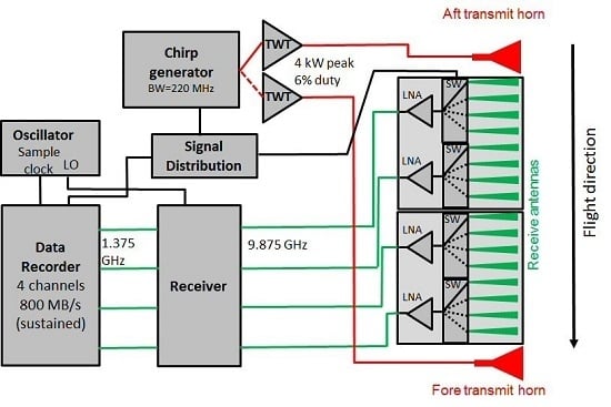
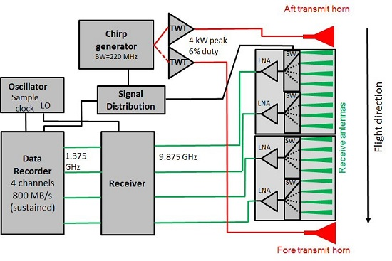
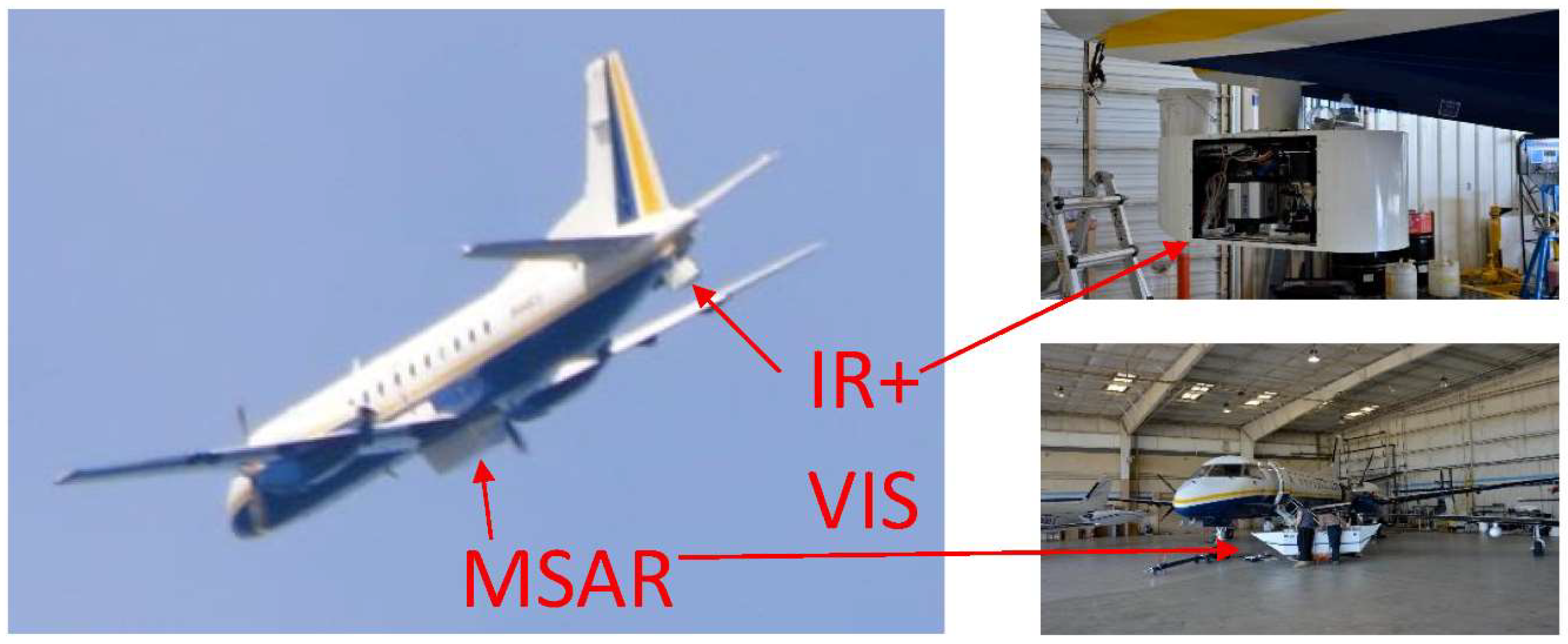
The objective of this study is to evaluate the ability of the airborne remote sensing to accurately measure ocean surface currents on spatial scales of 10 s to 1000 s of meters. For this purpose, the experiment described in this paper simultaneously employs some of the above-mentioned methodologies of ocean surface current retrieval, more specifically: (1) hyperspectral visible-near infrared (VNIR) imaging of fluorescent dye releases; (2) mid-wave infrared (MWIR) imaging of sea surface temperature modulations by subsurface turbulence; and (3) active microwave surface imaging with a Multichannel Synthetic Aperture Radar (MSAR). The study deals with many of the common challenges listed above, including an attempt to compare and validate against a bottom-mounted ADCP, as well as cross-comparison among various remote sensing products. The focus of the paper is on the technical details of the experimental setup and processing algorithms, which are given in Section 2. The resulting quantitative measurements of ocean currents obtained by the aircraft are presented, intercompared, and validated against ADCP in Section 3, followed by a discussion of the results, limits of their applicability, and associated uncertainties in Section 4.

2. Methodology

2.1. CASPER-East Experiment

The airborne remote sensing experiment described in this paper was conducted in collaboration with a larger multi-platform CASPER-East field campaign [16,31] conducted by an ONR (Office of Naval Research) funded Multidisciplinary University Research Initiative (MURI) titled “CASPER: Coupled Air-Sea Processes and Electromagnetic (EM) ducting Research”. The experiment took place in October and early November of 2015 off the coast of North Carolina, Eastward from the US Army Corps of Engineers Field Research Facility pier at Duck. The airborne surveys described here were conducted from a dedicated remote sensing research aircraft and were concentrated around an air-sea interaction supersite #2 (ASI2) established by CASPER approximately 63 km East from the shoreline (N36.1837, W75.0451), with the bottom depth at this location ≈38 m. The ASI2 supersite included permanently stationed (for the duration of the experiment) bottom-mounted ADCP (Manufacturer: Nortek, Rud, Norway; Model: Signature 500), vertical thermistor array mooring, vertically profiling underwater glider (Manufacturer: Webb Research, North Falmouth, USA; Model: Slocum) with temperature, salinity, and turbulence microstructure (Manufacturer: Rockland Scientific, Victoria, Canada; Model: MicroRider) probes, as well as a miniature wave buoy (by Scripps, La Jolla, USA). Additionally, ASI2 was frequently visited by two research vessels and another research aircraft, which resolved air-sea fluxes of momentum and heat, among many other environmental variables. Five flights by the remote sensing aircraft over the ASI2 were accompanied by a dye plume release from a small boat, which was also used to deploy and recover an autonomous underwater vehicle (Manufacturer: Hydroid, Pocasset, USA; Model: REMUS 100).

2.2. Remote Sensing Aircraft

A modified twin-engine aircraft (Manufacturer: Saab, Trollhättan, Sweden; Model: 340) was the remote sensing platform for the CASPER-East experiment. Typical speed of the aircraft during sampling was ≈70 ms⁻¹, and the altitude varied between 300 and 1400 m. The total sampling time over the ASI2 area was approximately 20 h of multiple flight days.

On the exterior, an array of microwave antennas (i.e., MSAR) was mounted under the belly of the aircraft, and visible and infrared sensors were mounted in a separate enclosure under the tail, see Figure 1. The visible sensors included three monochrome visible light cameras (Manufacturer: ImperX, Boca Raton, USA; Camera: CCD, 4872 × 3248, 3 fps) with polarization or dye-specific color filters, and a hyperspectral visible to near infrared pushbroom sensor (microSHINE, custom made), see more details on this sensor in the following section. The suite of infrared cameras included a short-wave infrared hyperspectral pushbroom imager, mid-wave infrared camera (Manufacturer: FLIR, Wilsonville, USA; Model: SC6000) and two long-wave infrared cameras (Manufacturer: Sofradir, Chatenay-Malabry, France; Model: ATOM 1024). All visible and infrared sensors were pointed close to nadir (average incidence angle ≈0°) except for one ImperX camera with a horizontal polarization filter and one long-wave infrared camera, both of which were pointed at ≈70° to the port side of the aircraft with the intention to co-locate with MSAR’s footprint.

Remaining subchapters describe in more detail a subset of instruments, accompanied by corresponding sampling strategies and processing algorithms, which were ultimately found most useful in producing outputs related to ocean currents. These outputs are, in turn, presented further in the Results section.

2.3. Visible Light

2.3.1. Dye Release

Dye plumes released ahead of the aircraft arrival at the ASI2 location served not only to boost the signal available to visible sensors, but also as a survey anchor point used by pilots for navigation. The dye plume was released in a straight line up to ≈10 km long and the aircraft flew directly above and along the plume, to make sure it is captured within narrow visible and infrared swaths. At the end of the plume, the aircraft turned around and flew parallel to the plume, so that the plume was approximately in the middle of the side-looking MSAR swath. This racetrack pattern was repeated approximately 10 to 15 times as the plume drifted and its shape evolved under the influence of turbulent currents.

A significant effort was undertaken to avoid plume motion contamination by the turbulence within boat’s wake. To minimize the wake, a dedicated small boat was used (a local fishing boat named “A-Salt Weapon” out of Oregon Inlet), which moved at the slowest speed (up to ≈2 ms⁻¹, depending on waves) necessary to maintain constant course. Furthermore, instead of pumping the dye into the water, it was mixed with saltwater and then sprayed into the airflow with the spray nozzle located at a ≈5 m height, above and away from the stern. The boat was always moving in a direction approximately perpendicular to the wind direction, so that the dye spray was introduced into an unobstructed airflow. The size of spray droplets was of the order of 10 s to 100 s µm, and only less than 1% of its initial volume consisted of dye. This ensured that once the droplet deposited on the water surface, it did not disturb the native surface turbulence: neither mechanically, nor through buoyancy effects, since the resulting dye concentration drops well below <1 ppm on contact, where its buoyancy effects can be neglected. Spraying dye also insured that the initial depth of the dye plume was zero, and that consequent entrainment was purely due to turbulent motions.

Figure 2 demonstrates a high-resolution example of such dye plume, as captured by one of ImperX cameras from the aircraft. It can be seen that immediately behind the boat the plume acquires small-scale streaking features oriented in the wind direction. Also, downwind boundary shape possesses feathers-like structure, unlike its smoother upwind counterpart. These initial small-scale distortions of the plume are thought to be primarily the result of turbulent airflow structures, which carried the spray from the nozzle to the point of deposition. Additionally, the boat (and the nozzle with it) rolled with the waves, which also could have contributed to initial unevenness of the plume’s structure. However, any evolution of the plume’s structure away from the immediate vicinity of the boat can be readily attributed to the effects of the upper ocean turbulence.

Airborne infrared imagery (not shown) revealed that the goal of separating the boat wake and the dye plume has been accomplished. Warmer than ambient turbulent wake of the boat was observed to be clearly separated from the colder than ambient dye plume. The boat’s wake is expected to be warmer due to the distortion of the cool skin layer by the wake turbulence, whereas colder dye plume is expected due to the deposition of dye spray particles, cooled by evaporation while airborne. The separating distance between the boat’s wake and the dye plume was observed to be anywhere between 10 and 40 m, mainly depending on the wind speed.

The primary dye used in this experiment was Uranine, which is a fluorescent water-tracing dye with the peak emission wavelength of 520 nm (green). The secondary dye was Rhodamine WT (i.e., Water Tracing) with peak emissions at 585 nm (red). Two down looking ImperX cameras were equipped with green and red filters, so that the two dyes could be visualized separately. Figure 2 showing the Uranine dye plume is an example of a raw image acquired by such camera with green filter. The two dyes sprayed at different times (first green, then red) over the same area are shown in Figure 3. Here a separate monochromatic camera imaged each dye, then red and green values were assigned, and images co-located in post processing to generate the figure. The red dye was released over some parts of the green dye with the objective to understand the inter-dependence between small-scale turbulent features highlighted by the fresh plume and larger scale turbulence, which had enough time to entrain the older plume. This two-dye analysis, however, is left for future work, whereas this paper focuses only on the Uranine dye plumes henceforward.

2.3.2. Visible Airborne Imagery of the Dye

Visible-near-infrared hyperspectral imagery collected with microSHINE (Small Hyperspectral Imager for Naval Environments) was the primary tool for imaging overall large-scale shape of dye plumes. MicroSHINE is a prototype version of the pushbroom sensor manufactured by Brandywine Optics, Exton, USA, model: CHAI V-640. It was configured to collect data spectrally in 160 bands from 273 to 1071 nm at 5 nm spacing, with usable data observed from ~400–900 nm. Pre and post-flight spectral, radiometric, and pointing calibrations were performed in the Naval Research Lab (NRL) calibration facility following methods described in [32,33]. MicroSHINE has a 48-degree field of view spread across 1360 cross-track pixels. Integration times and frame rates during the experiment varied between 10 and 100 ms and 9 to 35 Hz respectively. Flight altitude, frame rate, and speed during the experiment resulted in pixel sizes of between 1 and 5 m in along-track and 0.2 and 1.0 m in cross-track direction which were then resampled to 1 × 1 m square UTM (Universal Transverse Mercator) grid pixels during geolocation, which was performed with IDL/PARGE [34]. Position and attitude information were collected at 10 Hz with an integrated system manufactured by Systron Donner, Concord, USA, model: CMIGITS-III. No atmospheric correction was performed on the data due to the low flight altitude, but glint was corrected by following the method of [35].

To extract dye concentrations from background signals and interfering fluorescence signals of the Rhodamine and Uranine, a fluorescence line height (FLH) was calculated following an approach typically used to quantify phytoplankton fluorescence [36,37]. Briefly, a peak fluorescence wavelength was identified for each dye along with the shoulders of that peak outside of the influence of the fluorescence. A baseline is calculated by linear interpolation between bands outside the influence of the fluorescence and this baseline is then subtracted from the radiance measured at the peak fluorescence band, as follows

FLH = (L₂ − L₃) − [(λ₂ − λ₃)/(λ₁ − λ₃)] × (L₁ − L₃),

(1)

where L₁, L₂, and L₃ are radiances at the left shoulder, fluorescence peak, and right shoulder respectively and λ₁, λ₂, and λ₃ are the wavelength centers of the bands in L₁, L₂, and L₃.

Figure 4 shows an example of Uranine dye swaths collected at three different times as it drifts, and its shape evolves under the effects of surface currents. To further quantify these plume images, the location of the plume’s centerline was identified at every meter along the entire length of the plume. It was calculated using peak cross-covariance between a Uranine radiance cross-section and a Gaussian bell curve representative of a typical cross-section shape. Red dots in Figure 4 show resulting centerline locations along each visualization of the plume.

To reconstruct surface velocities along the plume, centerline locations are compared to the initial location and time of the dye release. Based on the knowledge of the exact time and location of plume release start and finish points, and on the fact that the boat moved with a constant speed and course while releasing the dye, it is possible to estimate the distance and the time that each parcel of the plume traveled (in cross-plume direction) to arrive at the measured centerline point. This gives a surface current velocity estimate U(y) at each meter along the length of the plume, where U is along-wind (cross-plume) component of the velocity and y is the cross-wind (along-plume) horizontal coordinate.

2.3.3. Limitations of Dye Plume Velocimetry

As will be shown further in the Results and Discussion sections, U(y) obtained continuously along many kilometers is a unique and valuable measurement. However, it comes with a multitude of assumptions and limitations, which are important to understand, to not overstep its limits of applicability. First important limitation to define is the smallest turbulent scale the plume can resolve. Although plume’s centerline and thus velocity estimate is given at each meter, the plume’s typical overall thickness is about 20 m. Here thickness is defined by the boundaries beyond which signal to noise ratio of the dye signal becomes too small to isolate the dye from background noise. This thickness remains surprisingly constant during the few hours of observations due to counteracting actions of dye dispersion and its photo degradation. Since the entire thickness of the plume weighs in on the location of the centerline, it is expected to dampen the effects of small scales at or below the order of 10 m. Moreover, the average time that the dye spent in the water was about 1 h, reaching 2 h in older parts of long plumes. This exceeds the eddy overturning time expected for eddies of 10 m or less, indicating that the velocity variability within these eddies might not be represented accurately and is likely dampened. The freshest (most recently sprayed) parts of the plume, on the other hand, have the opposite effect of unrealistically amplifying the turbulent kinetic energy (TKE) on the smallest scales. This is due to the imperfections in the initial shape of the plume discussed earlier is Section 2.3.1, which make the initial centerline non-straight. If very little time is given between the dye release and its observation from the aircraft, these initial imperfections will dominate or be comparable to consequent distortions by the true turbulence, which will lead to erroneously high kinetic energy on the small scales in the fresh part of the plume. This effect was evaluated by comparing TKE spectra of the same plume from multiple swaths, as the overall age of the plume grew (not shown). Indeed, the noise level on the small scales was found to be higher in fresher plumes, whereas the rest of the spectra remained unchanged from swath to swath. This effect, however, was found to disappear and the entire spectrum reached a quasi-equilibrium state once all data points were from the parts of the plume, that were at least 20 min old. Therefore, this requirement was imposed on all dye plume velocity estimates henceforward.

2.3.4. Vertical Structure of Dye Plumes

Another significant uncertainty associated with dye plume velocity estimates is related to the vertical entrainment of the dye. As was discussed in Section 1.4, it is critical to specify the depth to which a velocity estimate corresponds. The depth of the signal obtained by a passive airborne color sensor is related to the depth of the dye, but also inversely related to the clarity of the water. During this study it was estimated that approximately 90% of the measured signal originated from the top 10 m of the water column. To better understand and quantify the vertical structure of the dye plume within these top 10 m, this study employed an autonomous underwater vehicle (AUV) REMUS 100. In addition to the standard temperature, salinity, and depth sensors, it was equipped with a triplet (Manufactured by Sea-Bird Scientific, Bellevue, USA; Model: ECO Puck), which included a fluorometer designed to detect Uranine dye concentrations. To resolve vertical structure of the dye plume, the AUV was programmed to follow a straight line while making frequent vertical dives from 0 to 20 m depth in a sawtooth shape, see Figure 5b. Once the AUV was on course, the boat followed the same line and sprayed the dye ahead of the AUV. Boat’s velocity varied slightly (Figure 5a), causing variations in boat-AUV separation distance (Figure 5c), and thus allowing the AUV to sample various ages of the plume (Figure 5d). Due to underwater navigation uncertainties, combined with the plume’s drift unknown in real-time, it is extremely hard to ensure that the AUV samples inside of the plume (only ≈20 m wide), instead of moving parallel just outside of it. Figure 5e, shows the only successful attempt, in which AUV was indeed inside the plume and detected high concentrations of Uranine on many occasions.

The data collected by the AUV gives a unique insight into the early stages of the vertical development of the plume. By combining the age of the plume with a binary representation of a positive identification of Uranine presence, it is possible to track the entrainment of the dye in depth, see Figure 6. As expected, within the first minute or so, all the dye was found to be near the surface, where it was released. This remained to be the case for most of dye detection instances throughout the sampled range of ages. However, the AUV has also detected occasional downward intrusions of the dye, which grew in depth as the plume aged at a rate of approximately 3 cm s⁻¹ and reached as far as the depth of 12 m by the end of the 6th minute after the moment the dye was sprayed on the surface. This is consistent with the theory of Langmuir circulations, which expects occasional narrow convergence and downwelling regions with the maximum vertical velocity of 3 cm s⁻¹ in case of a stable upper ocean [38].

This ability of the upper ocean turbulence to rapidly entrain the dye within just 6 min leads to the conclusion that by the typical plume age observed by the aircraft (ranging from 20 min to 2 h), the dye was close to fully entrained across all vertical turbulent structures down to the base of the mixed layer (approximately 10 to 20 m in this study). Therefore, the horizontal displacement of the plume detected by the aircraft is more representative of a vertical mean of horizontal velocities across the mixed layer depth. This further indicates the plume’s inability to represent velocities of small-scale structures of the order of 10 m, due to their likely dependence on the depth, and suggests that horizontal plume velocities are only appropriate for measurements of larger scale two-dimensional flow structures with horizontal length scales much larger than the mixed layer depth.

2.4. Infrared

Among all infrared sensors installed on the aircraft, the mid-wave infrared camera (FLIR SC6000) produced the most useful imagery. This was due to weak relative fluctuations of the sea surface temperature (SST) available within the scene, which lead to the superiority of FLIR SC6000 with its low signal to noise cooled Indium Antimonide sensor (noise equivalent differential temperature of <18 mK) over other infrared sensors. The thermal calibration of this camera was done in laboratory conditions against a controlled temperature black body. Within the narrow range of measured sea surface temperatures, the calibration curve relating raw sensor signal to temperature measured in degrees K can be approximated by a linear polynomial fit (i.e., offset and gain coefficients). However, only relative temperatures are estimated within swaths using the gain coefficient. The absolute temperature measured by an airborne camera calibrated in a lab can differ from true SST measured in situ by a few degrees K. This is due to an additional offset imposed by a variety of poorly quantified environmental factors, such as sky radiance reflected from the ocean surface, vapor and aerosols within the atmospheric path, as well as changes in infrared lens radiation, which fluctuates with ambient temperature outside of aircraft. Therefore, it is a common practice to rely on an infrared camera to obtain a swath of relative SST fluctuations, but require an in situ sensor for offset correction. An example of a large-scale raw infrared swath of relative SST fluctuations is shown in Figure 7.

To further reduce the noise level of an infrared swath, the mid-wave sensor has an additional advantage of the short integration time of 2 ms, as opposed to typically longer times needed for long-wave infrared sensors. With the recorded frame rate of 60 Hz and 640 × 512 pixels covering ≈30° field of view, this allows for collection of tens of frames over each scene during a single pass. After geolocation and regridding of the imagery on the UTM square 1 × 1 m grid, this overabundance of frames allows averaging over at least 10 realizations for each grid point, thus driving the effective noise level further down (see Results section for examples of imagery with noise suppression).

2.5. Microwave

A block diagram of the NRL’s MSAR system is shown in Figure 8. The key feature of the system is an antenna configuration that produces 32 along-track phase centers, allowing the generation of 32 SAR images, spatially co-located but separated in time. As described below, these images can be combined interferometrically to produce a high-precision velocity image from which small-scale currents can be estimated. The 32 phase centers are produced by 2 transmit antennas in conjunction with a switched 16-element receive array. By alternately transmitting on the fore and aft antennas and receiving on 4 of the receive elements at a time, data from the 32 phase centers can be collected over the course of 8 pulses. The system uses a linear FM chirp waveform with a center frequency of 9.875 GHz and a bandwidth of 220 MHz to drive the two switched transmit channels, each consisting of a traveling wave tube amplifier (TWT) and a horn antenna. On the receiving side, 4 receive elements are sampled at a time by a 4-channel data recorder. Fast 4 × 1 RF switches route successive groups of 4 receive elements to the receiver from pulse-to-pulse. In this paper, only the 16 images produced using one of the transmit horns are considered, due to limited coherence with images produced using the other transmit channel. The system is deployed on the aircraft using a custom belly-mounted radome (see Figure 1). More information on the system can be found in [39].

The NRL MSAR was recently used to demonstrate Velocity-SAR (VSAR) imaging of the ocean surface [39,40]. While VSAR can effectively remove motion-induced distortion in maritime SAR imagery, its velocity resolution tends to be too coarse for imaging currents and the orbital motions of surface waves. Accordingly, in the present study, we adopt an alternative scheme for processing the MSAR data that provides a significant improvement in velocity precision, albeit a scheme that does not support the distortion correction possible with VSAR. This scheme is a modification of along-track interferometric SAR (ATI SAR) in which a high-precision interferogram is formed from the MSAR’s multiple phase centers. Specifically, the interferogram, ${\mathsf{\Gamma }}_1\left(x,y\right)$, is formed by coherently averaging the 15 individual, short-baseline interferograms produced by combining 16 adjacent MSAR images, two at a time:

$${\mathsf{\Gamma }}_1\left(x,y\right)=\overline{I_m\left(x,y\right)·I_{m+1}^{\ast }{\left(x,y\right)}_N} m=1:16$$

(2)

where $I_m\left(x,y\right)$ is the value of the kth MSAR image at the pixel located at (x,y). The brackets ${\langle ·\rangle }_N$ indicate averaging over N points in a neighborhood around (x,y) in each of the interferograms in the stack of 15 and the overbar indicates further averaging down the stack. We refer to this processing scheme as Multichannel ATI (MCATI) SAR. The interferometric velocity is then given by

$$V_{MCATI}\left(x,y\right)=\frac{L}{2\pi {\tau }_0}arg\left({\mathsf{\Gamma }}_1\right)$$

(3)

where ${\tau }_0=d_{pc}/V_p$ is the minimum interferometric lag of the system, d_pc is the phase center spacing, V_p is the platform ground speed, and $L$ is the radar wavelength. Both simulations and experimental analysis using NRL MSAR data indicate that MCATI processing produces a surface velocity precision (closely related to surface current precision) that is significantly better than that produced by other MSAR processing schemes [41]. In brief, MCATI achieves fine velocity resolution by using only the shortest baseline interferograms, which maximizes the correlation between the image pairs and thereby minimizes the interferometric velocity noise, and by increasing the number of independent interferometric velocity measurements at each resolution cell. The results presented in [41] indicate that these factors produce a velocity precision on the order of 5 cm/s, even with meter-scale spatial resolution. A more complete velocity precision analysis than that found in [41] is underway and will be reported in a separate publication.

2.6. Acoustic Doppler Current Profiler

An upward looking 500 kHz five beam ADCP (Nortek Signature 500) was positioned at the bottom, 38 m below water surface, co-located with the rest of instrumentation at the ASI2 supersite. Velocity profiles were binned at 1 m depth increments and recorded at 4 Hz rate continuously throughout the experiment. Beam data were filtered with a 20 s Hanning filter and subsampled to 10 s, and corrected for several degrees of pitch and roll from post deployment shifting of the mounted (not gimbaled) instrument. By combining beam velocities, horizontal velocities were formed, and then low-passed filtered with a Hanning filter to arrive at time series with one-minute sampling rate. Beam velocities and therefore derived horizontal velocities above 10 m depth were deemed contaminated by sidelobe interference, and are not discussed.

Velocity data collected by ADCP serves as a source of validation for the airborne surface current measurements in this study. To enable its use for that purpose, time series of point measurements collected by the ADCP were converted to a spatial velocity array. This was done by assuming Kolmogorov’s frozen turbulence hypothesis, where flow’s mean velocity was used to convert time steps between samples into spatial steps. This conversion, however, was allowed only in instances where mean velocity was at least 4 times greater than the standard deviation. Such spatial statistics were collected over two-hour segments, thus ensuring that the mean flow was large enough to sample sufficiently large ensembles of spatial scales over that period, while staying short of and avoiding contaminations by tidal periods. This conversion into spatial velocity arrays allowed spectral filtering based on length scale criteria used further.

Time series of the standard deviation of along-shore velocities with spatial scales over 100 but below 500 m measured at 10 m depth are shown in Figure 9. The figure shows that depending on weather conditions, tides, and other forcing factors, the intensity of typical turbulent fluctuations varied around a few cm/s. Next, Figure 10 gives vertical profiles consisting of all ADCP bins showing such standard deviations averaged over the entire period. Furthermore, the profile is shown separately for length scales below 100 m (red circles) and above 200 m (black asterisks). As was suggested in the introduction, on small scales the intensity of the upper ocean turbulence strongly depends on depth. As such, the figure shows that the turbulent intensity profile for <100 m scales has a well-expressed minimum at 25 m depth, which indicates two important points. First, there appears to be two sources of turbulent kinetic energy: one due to bottom friction, which dominates over 25–38 m range, another due to air-sea surface forcing, dominating over 0–25 m range. The separation between these two boundary layers is also suggested by observations of a sharp density gradient (not shown) seen in vertical temperature and salinity profiles. The second important feature of the small-scale velocity profile shown in Figure 10 is the acceleration and steepening of the profile from 25 to 10 m depths, which suggest likely continued accelerated increase of turbulent kinetic energy towards the surface. If so, the standard deviation values at 10 m depth (also shown in Figure 9) are likely to be several times smaller than the corresponding values at the surface. The exact shape to be expected from near-surface turbulent profiles, of course, has been a subject of many studies, e.g., [42], and its deviation from the classical Law of the Wall is debated to this day.

This study, on the other hand, is more concerned with larger scale turbulent features detected by the ADCP and by the aircraft. For example, recall Section 2.3, which suggests that dye tracing velocimetry is only applicable on scales much larger than the mixed layer depth. Turbulent structures on these larger scales primarily move in the horizontal 2D plane and are not expected to have strong dependence on depth. This point is demonstrated by the profile of large-scale turbulent velocities (black asterisks in Figure 10), which does not have a strongly expressed depth dependence. Our ADCP data analysis found that this depth dependence gradually disappears on the scales from 100 to 200 m, which thus becomes the lower bound of our length scale analysis hence after and enables cross-comparison between various velocity measurements on these scales within the upper ocean mixed layer.

The velocity power spectra, S_u(k) were calculated at the shallowest ADCP depth (10 m) for each two-hour segment and are shown both as a function of k [m⁻¹] and as a function of λ [m]. Here we depart from a conventional visualization of power spectra as a function of wavenumber, k, due to the widespread use and intuitively easier interpretation of λ on these scales. However, the relationship between the wave length and the wave number can be recovered simply as k = 2π/λ. Figure 11 shows power spectra realizations from each two-hour segment with scattered dots, which are then binned by length scale to produce bin-averaged spectral shape shown with red asterisks. Furthermore, a power law

S_u(k) [m³ s⁻²] = 0.7 × 10⁻⁴ × λ¹,

(4)

was fitted through bin averages to represent this average spectrum observed by ADCP. This power law is shown with dash-dotted line and appears further in various comparisons to velocity spectra obtained by airborne methods. Note, while power spectra realizations over shorter time durations were also available and preferable for comparisons to aircraft data, the severe limitation of ensemble size makes such short-term realizations highly noisy and hence uninformative.

3. Results

3.1. Dye Plume Velocimetry

Velocities obtained from dye plume tracking, as described in Section 2.3, were successfully obtained on five occasions during the experiment. Figure 12 shows turbulent velocities U(y) estimated for plumes released on the five days, as specified in the legend. Velocities shown here are not filtered and, therefore, include estimates of small-scale motions resolved at 1 m increments, as well as larger submesoscale turbulent structures. To isolate a range of scales, which is appropriate for dye tracking velocimetry and for comparison to ADCP data, plume velocities are further band passed between 100 and 500 m. Standard deviations of the remaining signals are taken and compared to the similarly calculated ADCP record, see red asterisks in Figure 9. Velocity power spectra taken over each of the five plumes are shown in Figure 13, where they are also compared to λ¹ (as in Equation (4)) and λ³ power laws.

3.2. Thermal Imaging

Figure 14 shows an example of two thermal swaths with enabled noise suppression (see methodology in Section 2.4). These two maps of the sea surface temperature were obtained by two consecutive overpasses ≈9 min apart over the same location. Images were spatially band passed to emphasize turbulent structures in the range of scales between 10 and 500 m. The thermal signal on this day (11 April 2015) was near detection limit, whereas it was below detection limit on other days. The straight and elongated nature of the raw imagery allows computing temperature spectrum along a very long (≈13 km) spatial array with sample spacing of 1 m. Such spectrum was calculated for each single row of pixels along a swath, then averaged over ≈100 rows, with the result shown in Figure 15. The figure shows power laws λ¹ and λ^5/3 for reference, although there is no expectation that the temperature spectrum should have similar slope as velocity spectrum.

A careful examination of turbulent structures revealed by the pair of swaths in Figure 14 shows multiple features present in both swaths, as well as their slight evolution. An application of Pattern Tracking Velocimetry algorithms, however, proved to be unsuccessful due to the lack of small-scale thermal features and low signal to noise ratio.

3.3. MSAR

Figure 16a shows an example of an original unfiltered MSAR velocity interferogram obtained using the methodology described in Section 2.5. Unlike visible (dye) and infrared signals, the velocity interferogram is a result of an instantaneous snapshot of surface velocities, which includes and dominated by small-scale surface gravity wave orbital motions on the order of 1 m/s. Without access to time series, wave and turbulent velocities on small scales are inseparable. Therefore, to remove wave signal and reveal surface current structure, averaging was done over a moving spatial window. The figure shows three attempted windows sizes (50 × 50, 100 × 100, and 200 × 200 m), with the wave signal appear to have been fully removed for the largest window size, thus revealing what is thought to be underlying submesoscale current structure.

Figure 17 shows 1D velocity spectrum calculated for each across-track (i.e., range) row of the original velocity interferogram and then averaged for the entire swath. To evaluate how much of the spectral energy belongs to wave motion, the figure also shows the power spectrum obtained from a co-located wave buoy. The λ¹ power law (as in Equation (4)) obtained from ADCP is also shown for reference.

4. Discussion

Each of the airborne remote sensing modalities demonstrated above was able to deliver a unique and valuable perspective on the structure and intensity of ocean surface currents along aircraft’s swaths. Here we present an evaluation and discussion of these results in their own right, but more importantly attempt to inter-compare them to expose important differences between various remote sensing techniques and validate retrieved velocities against in situ ADCP measurements. Two primary quantitative metrics used for these purposes across the paper are standard deviation of velocities, equally band passed over a range of length scales, and velocity power spectra. The slope of the power law that the spectra tend to follow is considered, as well as its absolute value.

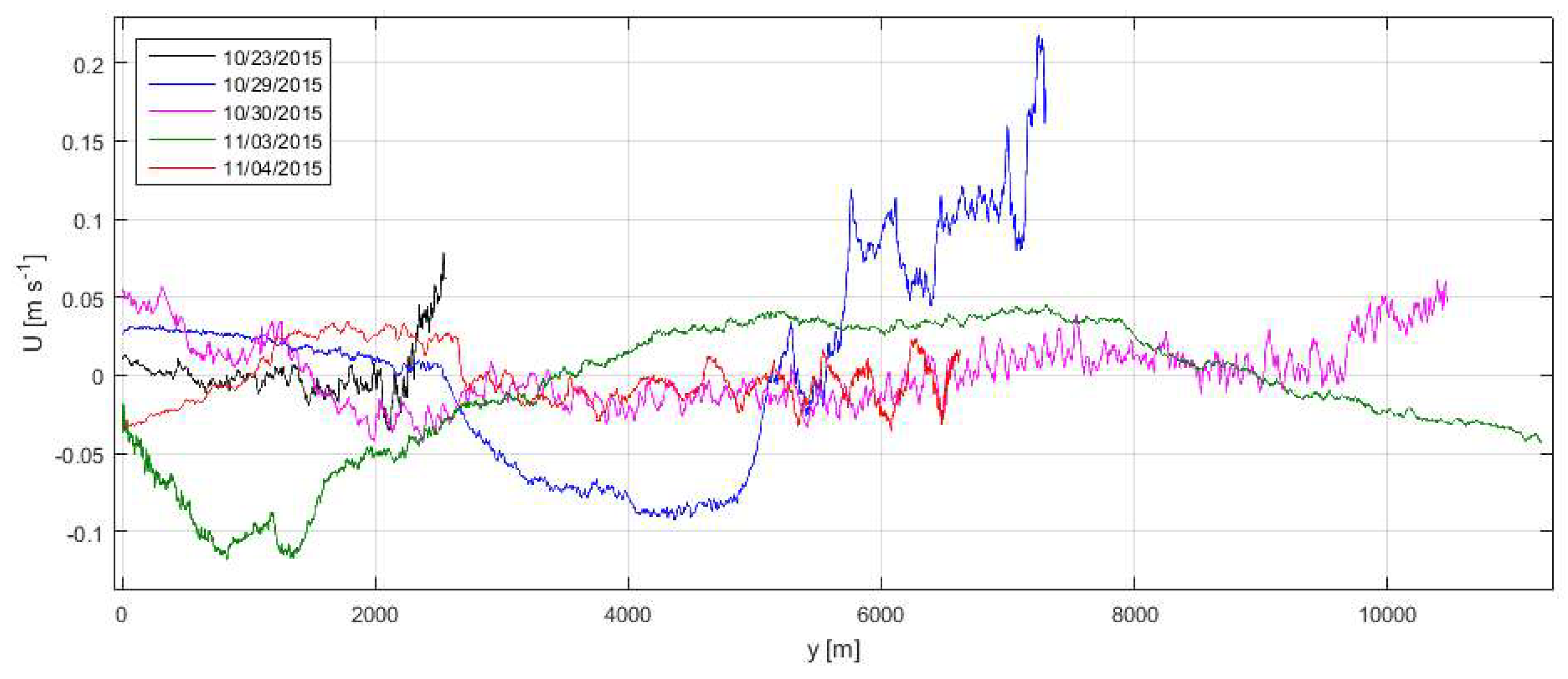
The smallest velocity scale resolved by the dye plume velocimetry has been estimated at around 100–200 m, or approximately 10 times the mixed layer depth (see Section 2.3.3 and Section 2.3.4). However, little attention has been given by the boundary layer turbulence community, nor by this paper so far, to the importance of the largest resolved length scale. The variability of velocity along plumes (Figure 12) clearly demonstrates the dominance of large submesoscale turbulent structures over smaller scale turbulence. This is further demonstrated by all turbulent spectra presented in this paper (Figure 11, Figure 13, Figure 15 and Figure 17), where the spectral energy sharply increases with length scale. Therefore, an estimate of the upper ocean turbulent kinetic energy is expected to be highly sensitive to the choice of the upper length scale limit. There does not appear to be a natural minimum indicating a separation between the small-scale turbulence presumably fed by surface forcing and larger submesoscale 2D turbulence, which is presumably fed by the energy cascading from even larger mesoscale oceanic currents, or other coastal mechanisms. Therefore, our choice of λ = 500 m for the upper limit is only motivated by sensor resolutions and ensemble sizes.

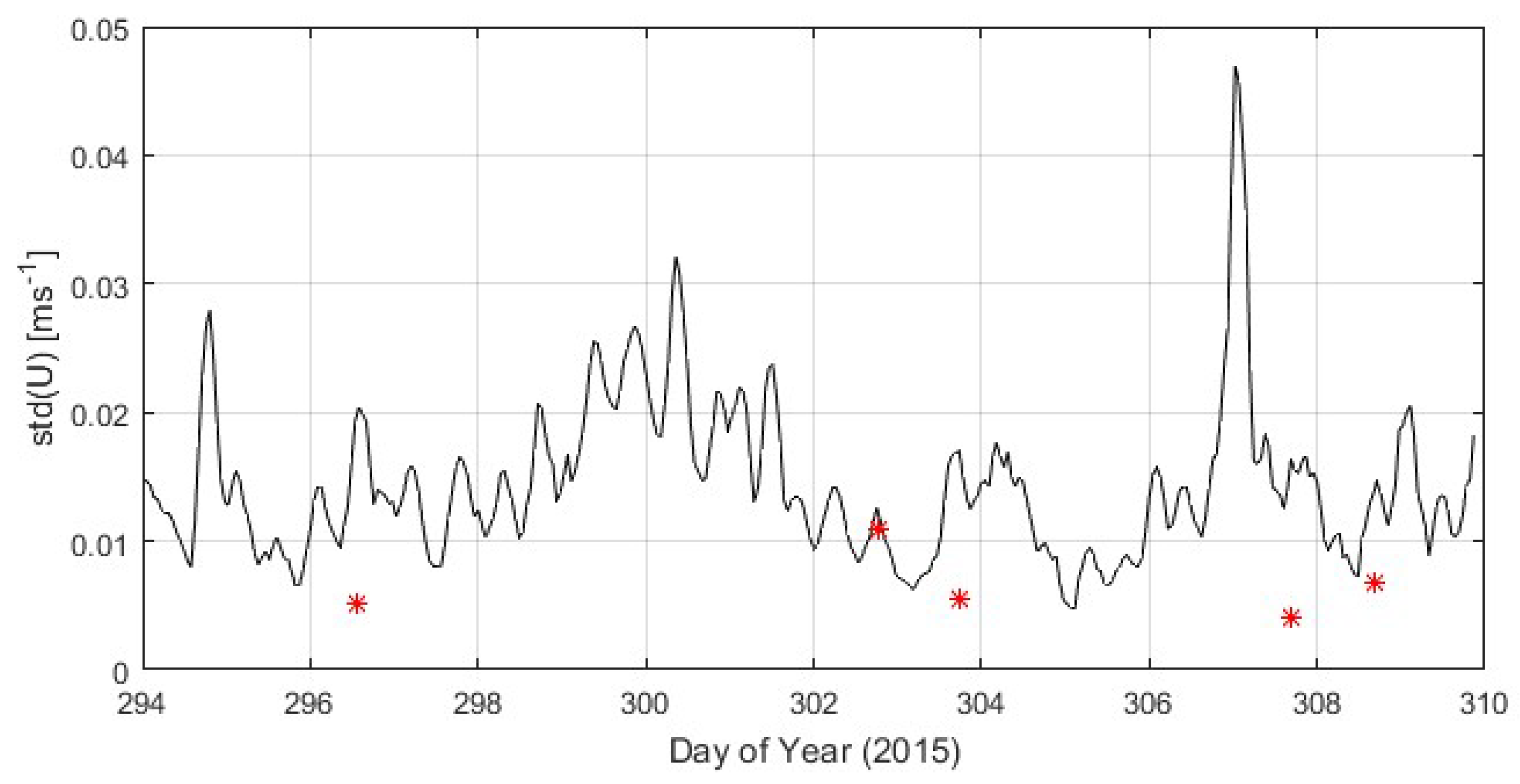
Having computed the TKE contained within the 100–500 m range, the results between the ADCP time series and five individual realizations from dye plume velocimetry are first compared in Figure 9. On all five occasions the airborne estimates are either nearly equal (once) or well below the ADCP estimate. An exact match between the two methods was not expected, as the ADCP might have been sampling a slightly different subsample of the flow from where the plume was located (typically within a several kilometer radius). However, the fact that none of the five aircraft realizations exceed ADCP values suggests a systematic bias. This could be in part due to measurement depth difference, where ADCP sampled at 10 m depth, whereas the dye plume velocity is sensitive to currents closer to the surface. However, that bias was mostly removed by filtering out small scales. If some bias remained, it would likely be larger, not smaller, favoring currents closer to surface, captured by the plume. More likely, the observed bias is due to the plume’s finite thickness and long time averages (discussed in more detail in Section 2.3), which results in the plume’s inability to resolve small-scale turbulent features. It is likely that some of that bias still exists in the 100–500 m range and thus causes lower values seen in Figure 9. 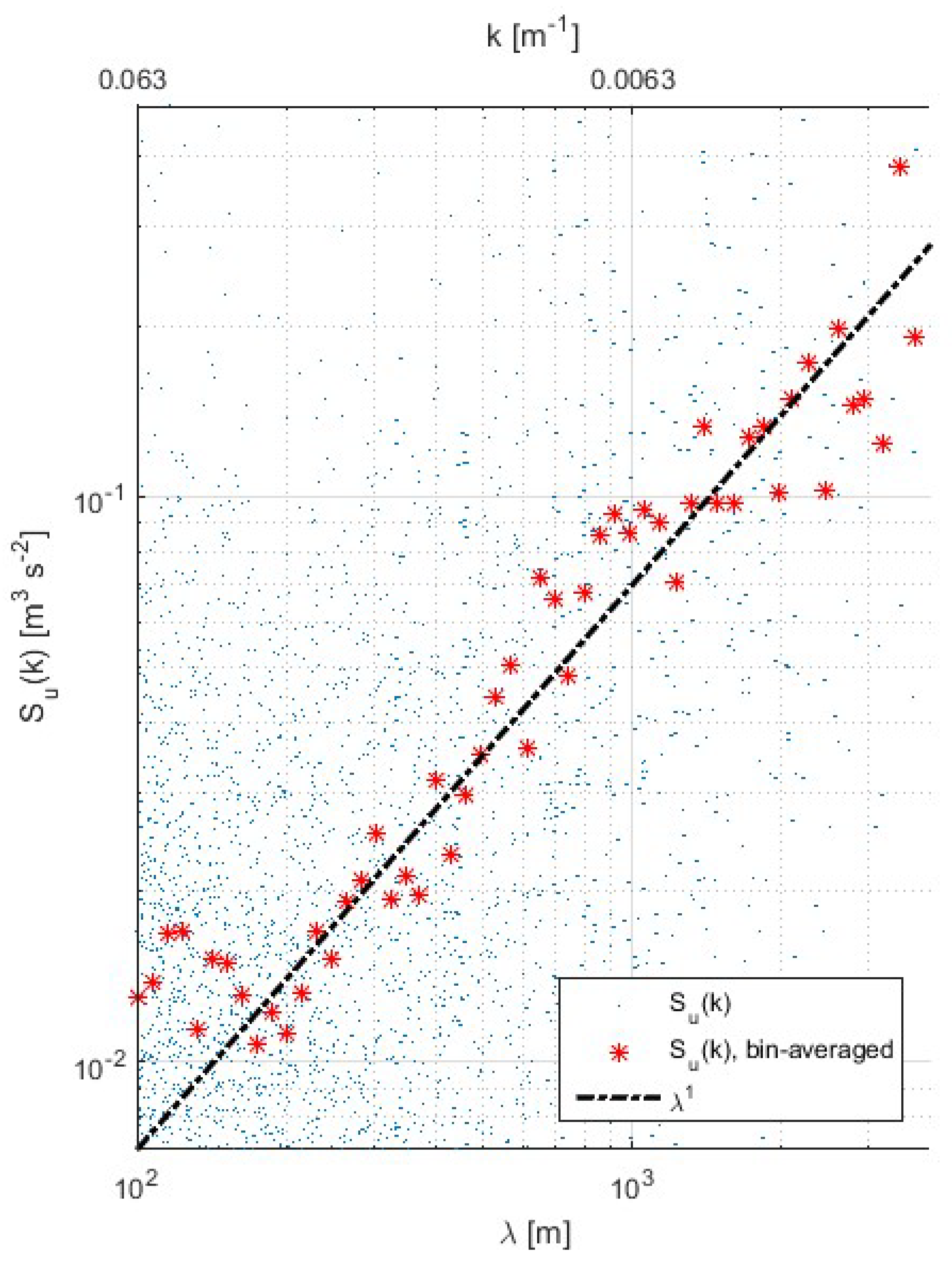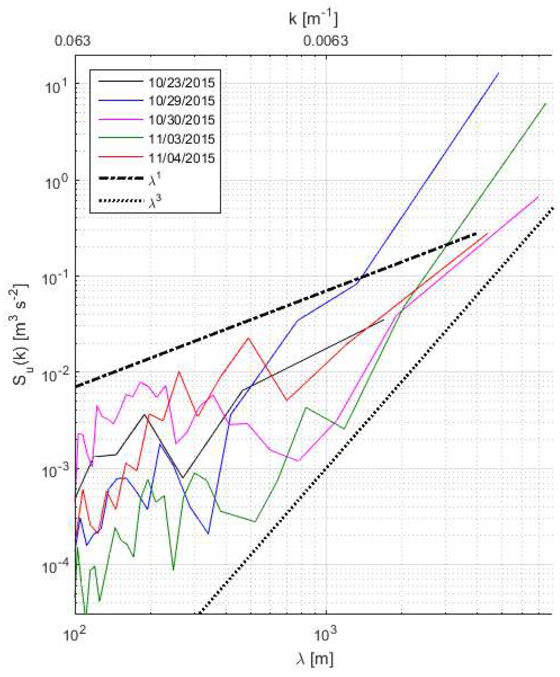This hypothesis is further supported by comparing velocity power spectra in Figure 13. On small scales, all five realizations of the TKE power spectra obtained from dye plumes start well below the average ADCP spectrum over that time frame, and proceed approximately parallel to the expected slope λ¹, although high levels of noise in these spectra make exact estimation problematic. However, by λ > 1000 m (or ×100 times the mixed layer depth), spectral levels catch up, indicating the gradual disappearance of the bias with length scale. Another interesting feature of these spectra at these larger scales (λ > 1000 m) is the apparent change of slope to λ³, perhaps indicating the start of the quasi-geostrophic turbulent cascade, known to follow that slope well into the mesoscales. For example, similar spectral slope and its flattening on smaller scales was suggested by [43].

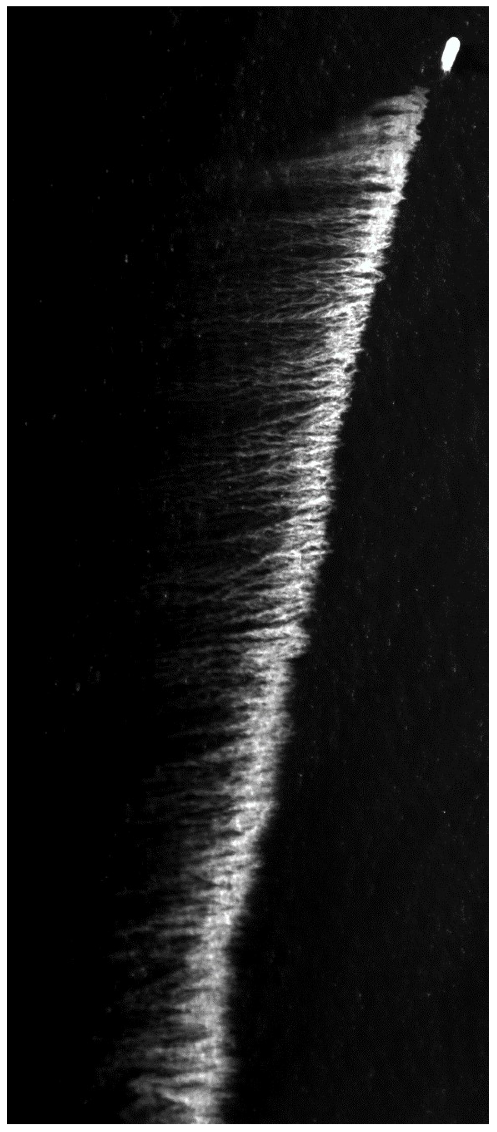
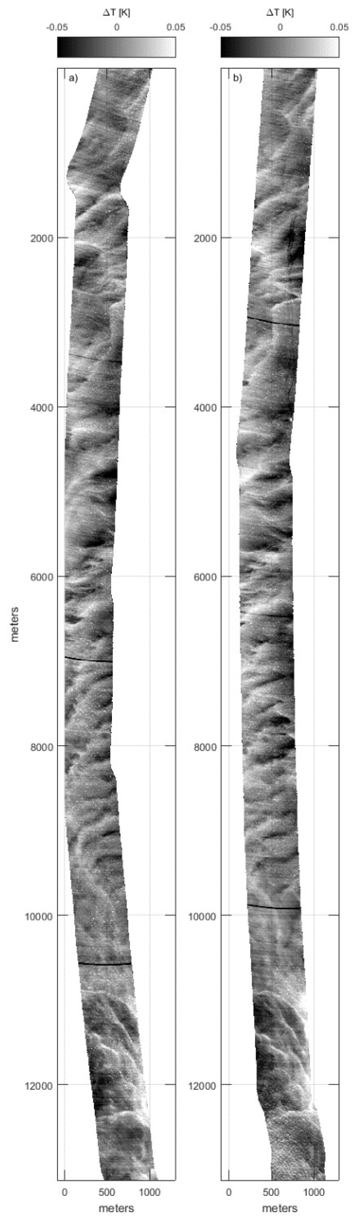
Our inability to convert infrared image pairs, such as Figure 14, into velocity fields is, of course, disappointing. Notably, in a similar experiment over a river, sufficiently feature-rich flow was observed with an airborne infrared sensor, its velocities estimated, and favorably compared to boat-mounted ADCP by [22]. The lesson learned here for future purposes is to take into consideration the expected availability of small-scale thermal contrast as a part of the experiment planning. The presence and the strength of small-scale thermal features needed for high fidelity Pattern Tracking Velocimetry, which in the open ocean primarily depends on the net air-sea heat flux, can and should be estimated and factored into go/no-go decision for an aircraft flight. 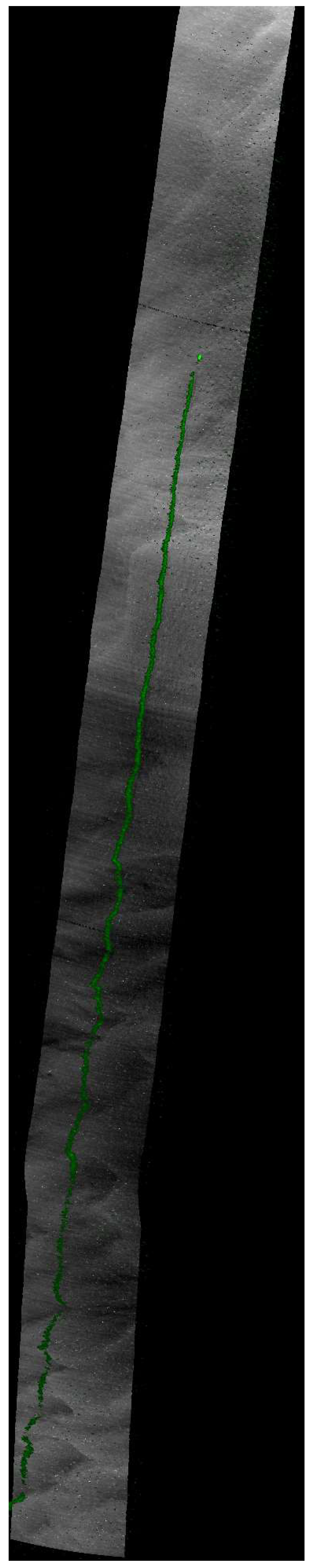Meanwhile, data contained in this study (e.g., Figure 14) can provide only qualitative information about the 2D spatial structure of the upper ocean turbulence. It reveals in detail the shapes, the typical length scales, the orientation, the anisotropy tendencies, and even widely disparate turbulent regimes (i.e., lower 4 km versus the rest of the swath) within the swaths. These images, unlike any other, demonstrate the immense complexity of the turbulent processes we are aiming to resolve and understand.

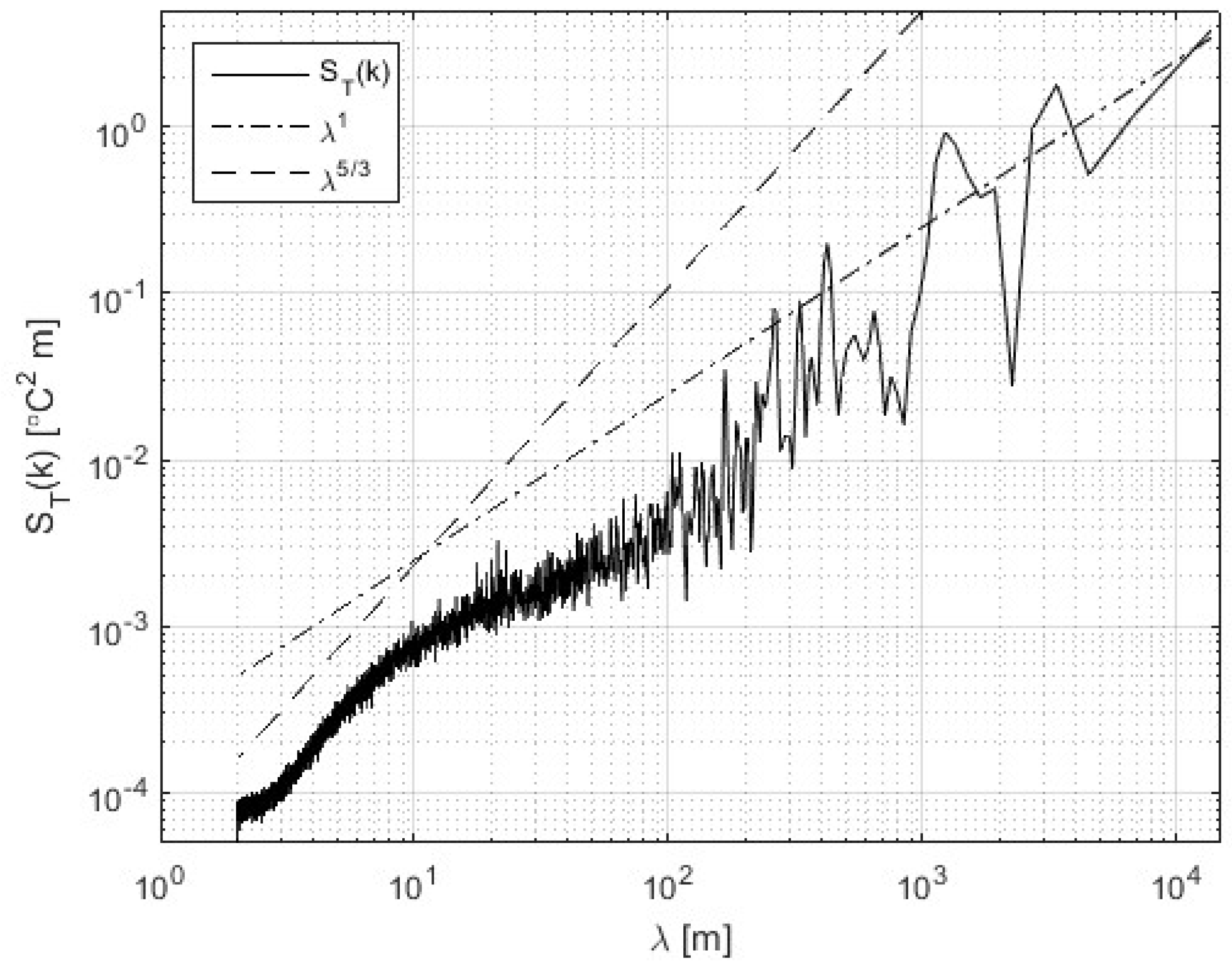
One useful quantity that can be obtained from these infrared swaths is the temperature power spectrum, shown in Figure 15. Unlike other airborne methods, 1 m is the true resolution of this dataset, and hence the unique feature of the obtained spectrum is the seamless connection across four orders of spatial scales from 1 m to 10 km. The spectrum apparently starts by following λ^5/3 power law on the smallest scales up to λ ≈ 10 m, then relaxes to ≈λ¹ for the rest of the resolved range. While it is tempting to suggest the correspondence to Kolmogorov’s 5/3 turbulent cascade on small scales and the correspondence to the λ¹ slope observed by the ADCP in Figure 11, there are no physical grounds to assume so. This would mean not only suggesting a proportionality between the magnitude of temperature and velocity fluctuations, but also suggesting that this proportionality coefficient holds constant across this vast range of resolved scales, which we can neither confirm nor deny based on the results of this study.

One way in which we envision thermal imagery can be used quantitatively is by means of numerical flow simulations. For example, if a Large Eddy Simulation model attempts to resolve upper ocean currents on these scales, it can solve for temperature as one of the unknowns. Then the model output can be used to generate similar surface temperature imagery, to compute temperature power spectra, which can then be compared to observations. Although not direct, a positive match will serve as a strong indirect indication that the velocity fields produced by the model are accurate as well.

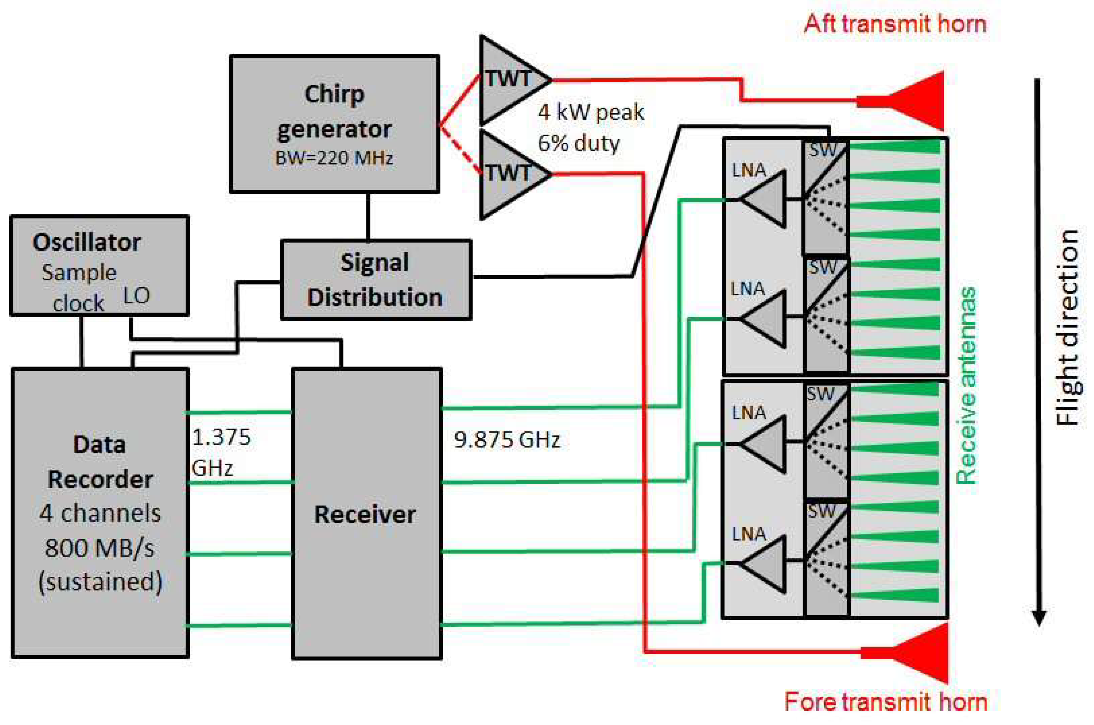
MSAR was able to obtain quantitative spatial maps of ocean surface velocities (cross-track component of the velocity vector) with approximately 10 m resolution and ≈5 cm/s velocity precision. Additionally, this paper represents a rare attempt to compare airborne interferometric SAR velocities to in situ data. The compared data sample is very limited, but valuable, as only few attempts of this kind were described in previous literature [28], leaving much room for a more comprehensive validation study in the future. 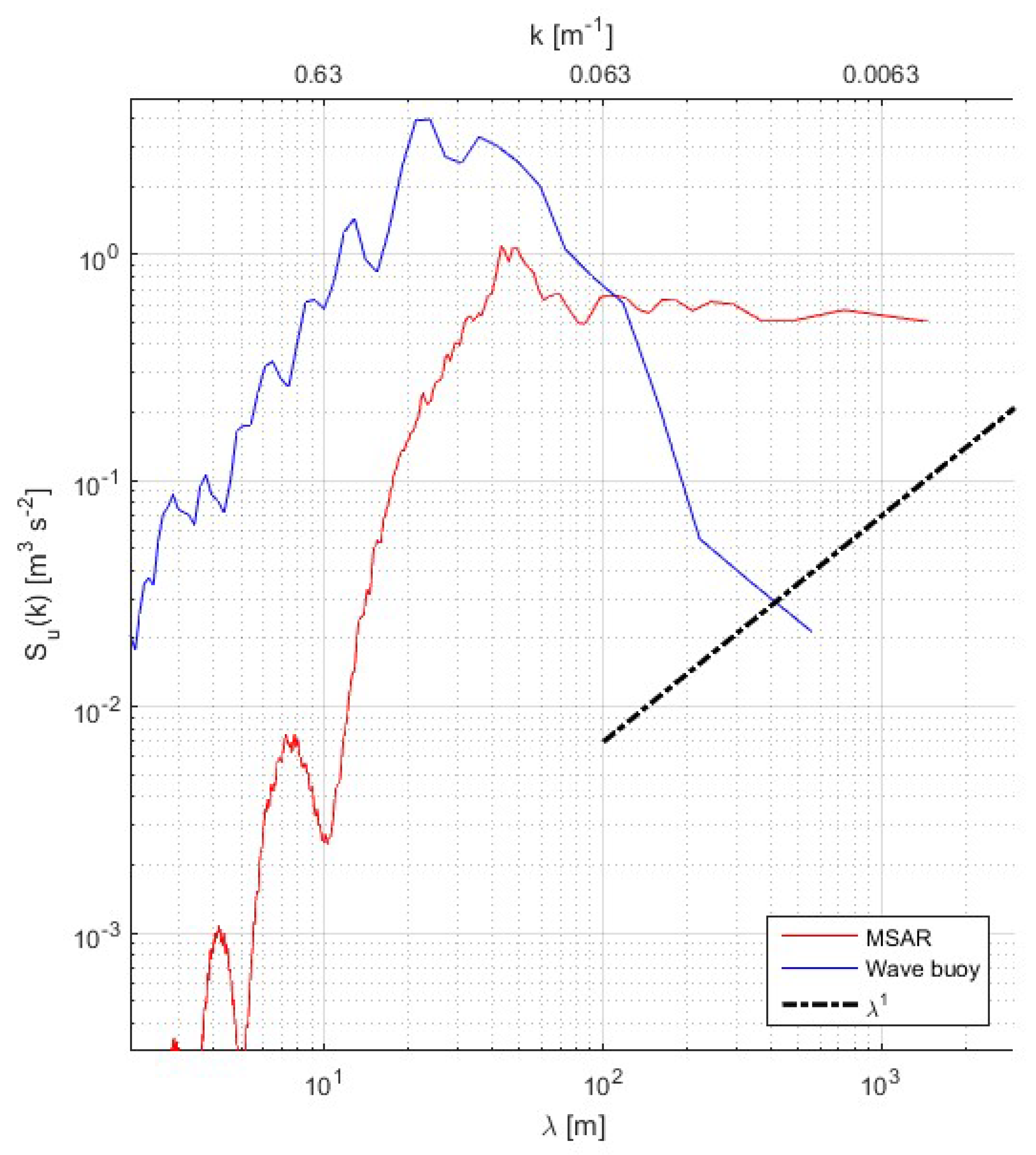Other most closely related active microwave current retrieval and validation studies employed methodologies based on offshore platform or ship-based marine radars and reported successful comparisons to bottom-mounted ADCP and surface drifters in situ velocity measurements [24,44]. Unlike other velocity estimates shown in this paper, MSAR obtains an instantaneous snapshot of true surface velocities (i.e., the velocity with which the surface carries ≈3 cm long capillary waves). Kinetic energy fluctuations observed by MSAR are expected to be stronger, due to the presence of the dominant wave energy and due to the sampling of the very top of the mixed layer, where the turbulence is expected to be more energetic than the rest of the water column, especially on smaller scales. Indeed, MSAR’s velocity power spectrum, shown with the red curve in Figure 17, places above the average ADCP spectrum. This contrasts with the dye plume velocimetry spectrum, which placed below the same ADCP spectrum on all but the largest spatial scales (recall Figure 13). However, once the wave energy spectrum is considered (blue curve in Figure 17), it appears that most of the small-scale energy in MSAR’s estimate comes from waves. The expected amount of wave energy is apparently underestimated, due to MSAR’s spatial resolution limitation of ≈10 m, causing it to miss some of the wave energy. Note, below 10 m a spatial filter was applied to MSAR’s interferogram to remove high wave number noise. A series of harmonics seen on the smallest scales of MSAR spectrum are primarily an artefact associated with that filtering. Both MSAR and wave buoy power spectra peak at a few tens of meters, after which they sharply diverge, indicating the rise of surface current contribution dominance. Therefore, it is the difference between MSAR and wave buoy spectra that is most indicative of the surface current spectra, and is indeed more in line with the λ¹ ADCP spectrum shown in the figure. Nonetheless, the absolute value of the MSAR spectrum appears to be noticeably larger than the ADCP, although that difference does appear to decline towards largest length scales. The swath width limitation does not allow resolving MSAR’s spectrum into larger scales, but if the observed trend persists, MSAR’s velocity spectrum is expected to intersect ADCP’s at λ equal to few kilometers, which is similar to where the dye plume spectrum of that day crossed the same ADCP curve (red line in Figure 13).

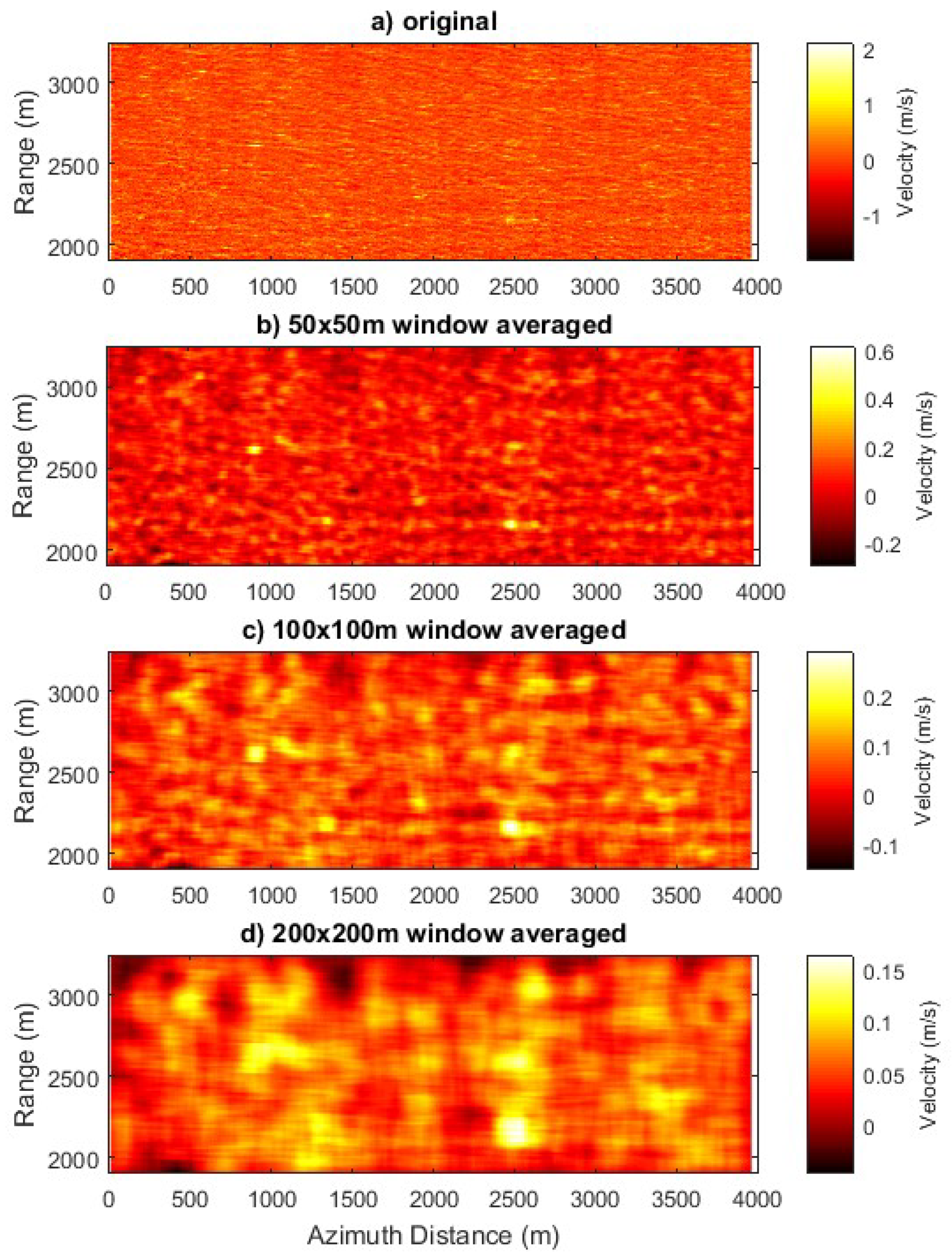
Large spatial filtering windows were applied to MSAR’s swath (Figure 16) to eliminate wave signal. It was able to reveal underlying currents only after the window size was increased up to 200 × 200 m. This is in line with the expectation based on the spectra in Figure 17, since the MSAR’s spectrum begins to predominantly consist of current energy only above λ > 200 m. Apart from the thermal swaths, the resulting filtered spatial image of MSAR’s surface currents (bottom panel of Figure 16) is the only other view into the 2D structure of submesoscale currents we were able to obtain. However, no detailed comparison between turbulent structures revealed by thermal and by MSAR swaths was undertaken here due to the fundamental differences in physical meanings behind these signals.

5. Conclusions

This paper presents an attempt at resolving upper ocean currents by means of various airborne remote sensing methods, including visible, infrared, and microwave bands of the EM spectrum. The airborne effort is accompanied by conventional underwater acoustic measurements of the vertical current profile, used to evaluate and validate the performance of airborne retrievals. The major conclusion is that airborne remote sensing methods can capture surface currents along the aircraft’s swath and thus provide a unique insight into the turbulent processes taking place on a wide and largely unresolved range of spatial scales between meters and tens of kilometers. However, these capabilities come with several important caveats and limitations, primarily related to turbulent length scale sensitivity and water depth sensitivity associated with specific airborne methods.

Visible band imagery of the upper ocean combined with a release of a long dye plume was found to be a powerful technique for resolving surface velocities and their power spectrum on the scales from ~100 to 10,000 m. However, the depth reference of retrieved velocities is uncertain, hence observed horizontal velocities are attributed to the overall horizontal motion of the mixed layer. Hence, this technique is limited to observations of 2D turbulence with length scales at least an order of magnitude greater than the depth of the mixed layer.

Infrared imagery was demonstrated to be a powerful tool for visualizing detailed 2D structure of the upper ocean turbulence. Additionally, it provided valuable surface temperature statistics in the form of a temperature spectrum on the scales from 1 to 14,000 m. However, its potential ability to produce surface velocity field was not realized due to insufficient signal to noise ratio in the small-scale thermal pattern.

The airborne MSAR combined with the new MCATI processing algorithm was able to resolve swaths of surface velocities (across-track component) with the unprecedented 10 m resolution and 5 cm/s accuracy. The resulting ≈1200 m wide interferogram swaths are instantaneous surface velocity snapshots, which contain turbulent current motions, but are also dominated by surface gravity wave orbital motions on small scales. A comparison to a co-located wave buoy spectrum, as well as spatial window filtering allows isolating submesoscale turbulence on the scales above the wave dominance, in this case λ > 200 m.

References

1. Dugan, J.P.; Piotrowski, C.C. Measuring currents in a coastal inlet by advection of turbulent eddies in airborne optical imagery. J. Geophys. Res. Oceans 2012, 117. [Google Scholar] [CrossRef] [Green Version]
2. Streßer, M.; Carrasco, R.; Horstmann, J. Video-Based Estimation of Surface Currents Using a Low-Cost Quadcopter. IEEE Geosci. Remote Sens. Lett. 2017, 14, 2027–2031. [Google Scholar] [CrossRef]
3. Laxague, N.J.; Özgökmen, T.M.; Haus, B.K.; Novelli, G.; Shcherbina, A.; Sutherland, P.; Guigand, C.M.; Lund, B.; Mehta, S.; Alday, M.; et al. Observations of Near-Surface Current Shear Help Describe Oceanic Oil and Plastic Transport. Geophys. Res. Lett. 2018, 45, 245–249. [Google Scholar] [CrossRef]
4. Holman, R.; Haller, M.C. Remote sensing of the nearshore. Annu. Rev. Mar. Sci. 2013, 5, 95–113. [Google Scholar] [CrossRef] [PubMed]
5. Hwang, P.A.; Sletten, M.A. Energy dissipation of wind-generated waves and whitecap coverage. J. Geophys. Res. Oceans 2008, 113. [Google Scholar] [CrossRef] [Green Version]
6. Langmuir, I. Surface motion of water induced by wind. Science 1938, 87, 119–123. [Google Scholar] [CrossRef] [PubMed]
7. Marmorino, G.O.; Smith, G.B.; Miller, W.D. Turbulence characteristics inferred from time-lagged satellite imagery of surface algae in a shallow tidal sea. Cont. Shelf Res. 2017, 148, 178–184. [Google Scholar] [CrossRef]
8. Ichiye, T. Upper Ocean Boundary-Layer Flow Determined by Dye Diffusion. Phys. Fluids 1967, 10, S270–S277. [Google Scholar] [CrossRef]
9. Sundermeyer, M.A.; Skyllingstad, E.; Ledwell, J.R.; Concannon, B.; Terray, E.A.; Birch, D.; Birch, D.; Cervantes, B. Observations and numerical simulations of large-eddy circulation in the ocean surface mixed layer. Geophys. Res. Lett. 2014, 41, 7584–7590. [Google Scholar] [CrossRef] [Green Version]
10. Marmorino, G.O.; Smith, G.B.; Lindemann, G.J. Infrared imagery of ocean internal waves. Geophys. Res. Lett. 2004, 31. [Google Scholar] [CrossRef] [Green Version]
11. Marmorino, G.O.; Smith, G.B.; Miller, W.D.; Bowles, J. Detection of a buoyant coastal wastewater discharge using airborne hyperspectral and infrared imagery. J. Appl. Remote Sens. 2010, 4, 043502. [Google Scholar] [CrossRef]
12. Marmorino, G.O.; Miller, W.D.; Smith, G.B.; Bowles, J.H. Airborne imagery of a disintegrating Sargassum drift line. Deep Sea Res. Part I Oceanogr. Res. Pap. 2011, 58, 316–321. [Google Scholar] [CrossRef]
13. Marmorino, G.O.; Smith, G.B.; Miller, W.D. Infrared remote sensing of surf-zone eddies. IEEE J. Sel. Top. Appl. Earth Obs. Remote Sens. 2013, 6, 1710–1718. [Google Scholar] [CrossRef]
14. Marmorino, G.O.; Smith, G.B.; Miller, W.D. Surface imprints of water-column turbulence: A case study of tidal flow over an estuarine sill. Remote Sens. 2013, 5, 3239–3258. [Google Scholar] [CrossRef]
15. Zappa, C.J.; Jessup, A.T. High-resolution airborne infrared measurements of ocean skin temperature. IEEE Geosci. Remote Sens. Lett. 2005, 2, 146–150. [Google Scholar] [CrossRef]
16. Savelyev, I.; Thomas, L.N.; Smith, G.B.; Wang, Q.; Shearman, R.K.; Haack, T.; Christman, A.J.; Blomquist, B.; Sletten, M.; Miller, W.D.; et al. Aerial observations of symmetric instability at the north wall of the Gulf Stream. Geophys. Res. Lett. 2018, 45, 236–244. [Google Scholar] [CrossRef]
17. Garbe, C.S.; Schimpf, U.; Jähne, B. A surface renewal model to analyze infrared image sequences of the ocean surface for the study of air-sea heat and gas exchange. J. Geophys. Res. Oceans 2004, 109. [Google Scholar] [CrossRef] [Green Version]
18. Dugan, J.P.; Anderson, S.P.; Piotrowski, C.C.; Zuckerman, S.B. Airborne infrared remote sensing of riverine currents. IEEE Trans. Geosci. Remote Sens. 2014, 52, 3895–3907. [Google Scholar] [CrossRef]
19. Chickadel, C.C.; Horner-Devine, A.R.; Talke, S.A.; Jessup, A.T. Vertical boil propagation from a submerged estuarine sill. Geophys. Res. Lett. 2009, 36. [Google Scholar] [CrossRef] [Green Version]
20. Johnson, E.D.; Cowen, E.A. Remote monitoring of volumetric discharge employing bathymetry determined from surface turbulence metrics. Water Resour. Res. 2016, 52, 2178–2193. [Google Scholar] [CrossRef] [Green Version]
21. Chickadel, C.C.; Talke, S.A.; Horner-Devine, A.R.; Jessup, A.T. Infrared-based measurements of velocity, turbulent kinetic energy, and dissipation at the water surface in a tidal river. IEEE Geosci. Remote Sens. Lett. 2011, 8, 849–853. [Google Scholar] [CrossRef]
22. Mied, R.P.; Chen, W.; Smith, G.B.; Wagner, E.J.; Miller, W.D.; Snow, C.M.; Marmorino, G.O.; Rhea, W.J. Airborne Remote Sensing of Surface Velocities in a Tidal River. IEEE Trans. Geosci. Remote Sens. 2018, 1–9. [Google Scholar] [CrossRef]
23. Marmorino, G.O.; Smith, G.B.; North, R.P.; Baschek, B. Application of airborne infrared remote sensing to the study of ocean submesoscale dynamics. Front. Mar. Sci. Under review.
24. Lund, B.; Haus, B.K.; Horstmann, J.; Graber, H.C.; Carrasco, R.; Laxague, N.J.; Laxague, N.J.; Novelli, G.; Guigand, C.M.; Özgökmen, T.M. Near-surface Current Mapping by Shipboard Marine X-band Radar: A Validation. J. Atmos. Ocean. Technol. 2018, 35, 1077–1090. [Google Scholar] [CrossRef]
25. Harlan, J.; Terrill, E.; Hazard, L.; Keen, C.; Barrick, D.; Whelan, C.; Howden, S.; Kohut, J. The integrated ocean observing system high-frequency radar network: Status and local, regional, and national applications. Mar. Technol. Soc. J. 2010, 44, 122–132. [Google Scholar] [CrossRef]
26. Goldstein, R.M.; Zebker, H.A. Interferometric radar measurement of ocean surface currents. Nature 1987, 328, 707–709. [Google Scholar] [CrossRef]
27. Toporkov, J.V.; Perkovic, D.; Farquharson, G.; Sletten, M.; Frasier, S.J. Sea surface velocity vector retrieval using dual-beam interferometry: First demonstration. IEEE Trans. Geosci. Remote Sens. 2005, 43, 2494–2502. [Google Scholar] [CrossRef]
28. Farquharson, G.; Deng, H.; Goncharenko, Y.; Mower, J. Dual-beam ATI SAR measurements of surface currents in the nearshore ocean. In Proceedings of the 2014 IEEE International Geoscience and Remote Sensing Symposium (IGARSS), Quebec City, QC, Canada, 13–18 July 2014; pp. 2661–2664. [Google Scholar] [CrossRef]
29. Hwang, P.A.; Toporkov, J.V.; Sletten, M.A.; Lamb, D.; Perkovic, D. An experimental investigation of wave measurements using a dual-beam interferometer: Gulf Stream as a surface wave guide. J. Geophys. Res. Oceans 2006, 111. [Google Scholar] [CrossRef] [Green Version]
30. Novelli, G.; Guigand, C.M.; Cousin, C.; Ryan, E.H.; Laxague, N.J.; Dai, H.; Haus, B.K.; Özgökmen, T.M. A biodegradable surface drifter for ocean sampling on a massive scale. J. Atmos. Ocean. Technol. 2017, 34, 2509–2532. [Google Scholar] [CrossRef]
31. Wang, Q.; Alappattu, D.P.; Billingsley, S.; Blomquist, B.; Burkholder, R.J.; Christman, A.J.; Creegan, E.D.; de Paolo, T.; Eleuterio, D.P.; Fernando, H.J.S.; et al. CASPER: Coupled Air-Sea Processes and Electromagnetic (EM) ducting Research. Bull. Am. Meteorol. Soc. 2017. [Google Scholar] [CrossRef]
32. Lucke, R.L.; Corson, M.; McGlothlin, N.R.; Butcher, S.D.; Wood, D.L.; Korwan, D.R.; Li, R.-R.; Snyder, W.A.; Davis, C.O.; Chen, D.T. Hyperspectral imager for the coastal ocean: Instrument description and first images. Appl. Opt. 2011, 50, 1501–1516. [Google Scholar] [CrossRef] [PubMed]
33. Bowles, J.H.; Korwan, D.R.; Montes, M.J.; Gray, D.J.; Gillis, D.B.; Lamela, G.M.; Miller, W.D. Airborne system for multispectral, multiangle polarimetric imaging. Appl. Opt. 2015, 54, F256–F267. [Google Scholar] [CrossRef] [PubMed]
34. Schlapfer, D.; Richter, R. Geo-atmospheric processing of airborne imaging spectrometry data. Part 1: Parametric orthorectification. Int. J. Remote Sens. 2002, 23, 2609–2630. [Google Scholar] [CrossRef]
35. Hedley, J.; Harborne, A.; Mumby, P. Simple and robust removal of sun glint for mapping shallow-water benthos. Int. J. Remote Sens. 2005, 26, 2107–2112. [Google Scholar] [CrossRef]
36. Gower, J.F.R.; Borstad, G.A. Mapping of phytoplankton by solar-stimulated fluorescence using an imaging spectrometer. Int. J. Remote. Sens. 1990, 11, 313–320. [Google Scholar] [CrossRef]
37. Letelier, R.M.; Abbott, M.R. An analysis of chlorophyll fluorescence algorithms for the Moderate Resolution Imaging Spectrometer (MODIS). Remote Sens. Environ. 1996, 58, 215–223. [Google Scholar] [CrossRef]
38. Myer, G.E. Structure and Mechanics of Langmuir Circulations on a Small Inland Lake. Ph.D. Thesis, The State University of New York, Albany, NY, USA, 1971. [Google Scholar]
39. Sletten, M.A.; Rosenberg, L.; Menk, S.; Toporkov, J.V.; Jansen, R.W. Maritime Signature Correction with the NRL Multichannel SAR. IEEE Trans. Geosci. Remote Sens. 2016, 54, 6783–6790. [Google Scholar] [CrossRef]
40. Jansen, R.; Raj, R.; Rosenberg, L.; Sletten, M. Practical Multi Channel SAR Imaging in the Maritime Environment. IEEE Trans. Geosci. Remote Sens. 2018, 56, 4025–4036. [Google Scholar] [CrossRef]
41. Sletten, M.; Toporkov, J. An Interferometric Approach to Ocean Surface Velocity Imaging Using Multi-Channel SAR. In Proceedings of the 2017 IEEE International Geoscience and Remote Sensing Symposium (IGARSS), Fort Worth, TX, USA, 23–28 July 2017; pp. 91–94. [Google Scholar] [CrossRef]
42. Terray, E.A.; Donelan, M.A.; Agrawal, Y.C.; Drennan, W.M.; Kahma, K.K.; Williams, A.J.; Hwang, P.A.; Kitaigorodskii, S.A. Estimates of kinetic energy dissipation under breaking waves. J. Phys. Oceanogr. 1996, 26, 792–807. [Google Scholar] [CrossRef]
43. Callies, J.; Ferrari, R.; Klymak, J.M.; Gula, J. Seasonality in submesoscale turbulence. Nat. Commun. 2015, 6. [Google Scholar] [CrossRef] [PubMed]
44. Huang, W.; Carrasco, R.; Shen, C.; Gill, E.W.; Horstmann, J. Surface current measurements using X-band marine radar with vertical polarization. IEEE Trans. Geosci. Remote Sens. 2016, 54, 2988–2997. [Google Scholar] [CrossRef]
Figure 1. (left) Photograph of the remote sensing aircraft SAAB 340 with (upper right) infrared and visible sensors enclosure and (lower right) MSAR radome.
Remotesensing 10 01224 g001
Figure 2. Visible high-resolution image of the Uranine dye plume in its early stage after the release. The dye boat in the upper right corner is ≈17 m long.
Remotesensing 10 01224 g002
Figure 3. Overlapping Uranine and Rhodamine dye plumes obtained by two high-resolution monochrome cameras (ImperX) with green and red filters.
Remotesensing 10 01224 g003
Figure 4. Three consecutive swaths over the same Uranine dye plume overlaid on one image. Greyscale shows the intensity of the Uranine dye signal, red dots follow the centerline of the plume. Horizontal and vertical axes correspond to relative Easting and Northing in meters.
Remotesensing 10 01224 g004
Figure 5. The figure shows various measurements related to or made by the REMUS 100 AUV as a function of its mission time: (a) The velocity of the boat, as it was releasing the dye ahead of the AUV’s track; (b) AUV’s depth; (c) relative distance between the boat the AUV; (d) effective age of the plume sampled by the AUV; (e) raw counts of Uranine, as measured by AUV’s fluorometer.
Remotesensing 10 01224 g005
Figure 6. Depth of the AUV (as in Figure 5b) versus effective plume’s age (as in Figure 5d) shown only for the instances with Uranine signal (Figure 5e) above noise level. The figure demonstrates the vertical entrainment of the dye (initially sprayed on the surface) by downward jets at a rate of ≈3 cm/s.
Remotesensing 10 01224 g006
Figure 7. A raw infrared swath (greyscale) overlaid with a visible image of the Uranine dye plume (green). See Section 3.2 for dimensions and temperature color bar definitions.
Remotesensing 10 01224 g007
Figure 8. MSAR block diagram.
Remotesensing 10 01224 g008
Figure 9. Standard deviation of the turbulent velocity on the scales between 100 and 500 m. Black line corresponds to ADCP measurements at 10 m depth, red asterisks are airborne dye plume velocimetry estimates.
Remotesensing 10 01224 g009
Figure 10. Time averaged vertical profiles of turbulent intensities measured by ADCP. Black asterisks curve corresponds to large-scale motions with length scales above 200 m, red circles curve corresponds to small scales (<100 m).
Remotesensing 10 01224 g010
Figure 11. Velocity power spectrum obtained by ADCP at 10 m depth. Blue dots are individual realizations obtained over two-hour segments throughout the length of the experiment. Red asterisks are bin averages of all spectra, each corresponding to an average of all realizations within a segment of the length scale λ. Dash-dotted line is an approximate fit to bin-averaged values, given by Equation (4).
Remotesensing 10 01224 g011
Figure 12. Values of across-plume velocities U given at every meter along the plume, starting with the oldest end of each plume at y = 0. Five curves correspond to five different plumes surveyed on different days, specified in the legend.
Remotesensing 10 01224 g012
Figure 13. Velocity power spectra calculated based on the dye plume velocimetry shown in Figure 12. Dash-dotted curve is the same as in Figure 11 and Equation (4). A λ3 power law is given for reference with a dotted line.
Remotesensing 10 01224 g013
Figure 14. Two consecutive infrared swaths (9 min apart) over nearly the same patch of the ocean surface, taken on 4 November 2015 simultaneously with dye visualization (see raw image in Figure 7). The signal’s noise is suppressed by averaging over 10 frames for each pixel and by band pass filtering between 10 and 500 m.
Remotesensing 10 01224 g014
Figure 15. Temperature power spectrum calculated along raw infrared swaths (same swath as in Figure 7 and Figure 14). Power law slopes of λ1 and λ5/3 are given by dash-dotted and dashed lines for reference.
Remotesensing 10 01224 g015
Figure 16. The figure shows original MSAR interferogram (a), and its smoothing as it is subjected to square window filtering of increasing size (b) 50 × 50, (c) 100 × 100, and (d) 200 × 200 m. Note, the color corresponds to across-track (i.e., range direction) velocity vector component, whereas the aircraft travels in the azimuthal direction.
Remotesensing 10 01224 g016
Figure 17. The red curve shows MSAR interferogram velocity (Figure 16, top panel) power spectrum in across-track (range) direction, averaged along realizations in the azimuthal direction. Blue curve shows wave energy obtained from a co-located wave buoy. Dash-dotted line gives the λ1 power law, same as in Figure 11 and Equation (4).
Remotesensing 10 01224 g017