Three-Dimensional Reconstruction of Soybean Canopies Using Multisource Imaging for Phenotyping Analysis

1
College of Electrical and Information, Heilongjiang Bayi Agricultural University, DaQing 163319, China
2
College of Agronomy, Heilongjiang Bayi Agricultural University, DaQing 163319, China
*
Author to whom correspondence should be addressed.
Remote Sens. 2018, 10(8), 1206; https://doi.org/10.3390/rs10081206
Submission received: 11 June 2018
/
Revised: 29 July 2018
/
Accepted: 30 July 2018
/
Published: 1 August 2018
(This article belongs to the Special Issue Estimation of Crop Phenotyping Traits using Unmanned Ground Vehicle and Unmanned Aerial Vehicle Imagery)
Abstract
:Geometric three-dimensional (3D) reconstruction has emerged as a powerful tool for plant phenotyping and plant breeding. Although laser scanning is one of the most intensely used sensing techniques for 3D reconstruction projects, it still has many limitations, such as the high investment cost. To overcome such limitations, in the present study, a low-cost, novel, and efficient imaging system consisting of a red-green-blue (RGB) camera and a photonic mixer detector (PMD) was developed, and its usability for plant phenotyping was demonstrated via a 3D reconstruction of a soybean plant that contains color information. To reconstruct soybean canopies, a density-based spatial clustering of applications with noise (DBSCAN) algorithm was used to extract canopy information from the raw 3D point cloud. Principal component analysis (PCA) and iterative closest point (ICP) algorithms were then used to register the multisource images for the 3D reconstruction of a soybean plant from both the side and top views. We then assessed phenotypic traits such as plant height and the greenness index based on the deviations of test samples. The results showed that compared with manual measurements, the side view-based assessments yielded a determination coefficient (R2) of 0.9890 for the estimation of soybean height and a R2 of 0.6059 for the estimation of soybean canopy greenness index; the top view-based assessment yielded a R2 of 0.9936 for the estimation of soybean height and a R2 of 0.8864 for the estimation of soybean canopy greenness. Together, the results indicated that an assembled 3D imaging device applying the algorithms developed in this study could be used as a reliable and robust platform for plant phenotyping, and potentially for automated and high-throughput applications under both natural light and indoor conditions.

1. Introduction
Soybeans are one of the main cash crops worldwide. To meet the needs of the growing human population, plant scientists and breeders must increase the productivity and yield of soybean crops, which is a substantial challenge [1]. High-throughput phenotyping platforms are essential for tracking the growth of soybean plants in the field and the contributions of these plants to both the food supply and the generation of bioenergy from their biomass [2]. Plant phenotyping involves the comprehensive assessment of plant characteristics that result from genetic and environmental factors [3,4,5,6]. Phenotypic characteristics include external morphological parameters such as plant height, size, petiole length, and initiation angle, as well as internal properties such as chlorophyll and nutrient (nitrogen, phosphorus, and potassium) contents [7,8]. The measurement and evaluation of these phenotypic traits can provide guidelines for plant breeding. However, most of the plant phenotyping methods depend on observations and manual measurements with contact sensors; these methods are considered low throughput, costly, and labor-intensive [9]. Furthermore, these traditional techniques typically require the destruction of plant organs, which negatively affects the normal growth of the measured plants [10]. Alternatively, plant phenotyping, which involves noninvasive measurements, is an emerging technology that has recently attracted the attention of researchers in the plant science and agricultural fields.
A current bottleneck that restricts phenotyping analysis lies in the development of the noninvasive and automated calculation methods that quantify the phenotypic traits of plants. In this regard, computer vision technologies show great potential for noninvasive measurement methods [11,12]. Currently, by recording whole three-dimensional (3D) datasets and reconstructing entire plants, 3D laser scanners can be used to acquire highly detailed plant phenotypic information on geometric traits, such as plant height. Photogrammetric information can be obtained via several different 3D techniques and laser devices, such as handheld laser scanners [13]. 3D plant models can then be generated by multiview stereo algorithms or by structure from motion [9,14]. Having very high resolutions, these techniques also present disadvantages, such as sensitivity to occlusion, a lack of color information, and failure to accurately reflect important phenotypic traits. Moreover, for the automatic phenotypic analysis of plant structure, 3D point clouds generated by laser scanners must be properly extracted from a large amount of 3D data, and must be classified. In addition, the high cost and limited availability of laser scanning devices have prevented their widespread application.
In addition to geometric traits, spectral reflectance in visible spectrum is another important characteristic for phenotyping analysis, especially for diagnosing nutrient conditions. Significant correlations between “soil and plant analyzer development (SPAD)” readings, leaf N concentration (LNC), and image color indices in RGB color space were observed for rice in natural light conditions [15]. Additionally, the strong relationship between the deficiency of nitrogen, phosphorus, potassium, and image color indices in RGB color space was further proved for soybean plants in an outdoor environment [16]. Although light intensity is one of the major factors that lead to color distortion, this kind of distortion can be registered by reference-based approaches to a great degree [17].
The above-mentioned studies showed that the nutrient conditions of plants of different cultivars and at different growth stages can be estimated in an effective way, that is, by using R, G, and B channel values that can be obtained by low-cost RGB cameras, without a wet lab, field-based sensors, or expensive image acquisition equipment.
Currently, geometric and spectral characteristics are acquired separately by different devices. With respect to agricultural applications, the spectral reflectance of plants’ canopies can be obtained by using an RGB-based camera or a multispectral camera [18,19], whereas the geometric information therein, such as plant height and canopy width, can be calculated via 3D cloud points generated by using 3D imaging devices such as terrestrial laser scanners or handheld laser scanners. Although some devices such as Kinect sensors [20] can capture image information (i.e., RGB images) and 3D distance information simultaneously, these two types of information cannot be acquired within the same coordinate system. Consequently, to obtain 3D plants with color information, a coordinate transformation is further required to be performed on these two types of information, thereby fusing multisource images. However, few techniques integrated with image fusion have been developed for the phenotyping analysis of plants, especially for soybean plants. Thus, there is still an urgent need in 3D reconstruction for plant canopies with both geometric and color information.
Although soybean plants are globally important crops for providing oils, most studies on reconstruction and phenotyping have focused on a single plant in a laboratory circumstance, such as a plant grown in a greenhouse [21]. These laboratory-based systems can be useful for obtaining certain phenotypic traits such as plant height, but they also have limitations. The main shortcoming is that certain traits calculated from an individual plant can not reflect the true cases in the field due to the artificial laboratory environment, which can significantly affect plant growth. Thus, phenotyping methods under natural light conditions are highly desirable for plant breeding. However, in contrast with progress made in laboratory-based research [22], the lack of a well-constructed platform has hindered the development of plant phenotyping under natural light conditions in large plantations. Therefore, there is a great opportunity for innovation with respect to the development of 3D-based technology for plant phenotyping under natural growing conditions.
To address these issues, it is demonstrated in this paper that it is feasible to reconstruct the 3D geometric characteristics containing the color information of soybean plants under natural light conditions by using a relatively low-cost multisource imaging system. This reconstruction was carried out through the efficient extraction and registration of multisource images by using density-based spatial clustering of applications with noise (DBSCAN), principal component analysis (PCA), and iterative closest point (ICP) algorithms. Our approach resulted in the successful characterization of soybean plant phenotypic traits (plant height and greenness index) acquired from 3D reconstructed images. This technique provides an alternative for the large-scale characterization of plant phenotypes under natural conditions.
2. Materials and Methods
2.1. Overall Process Flow for 3D Reconstruction
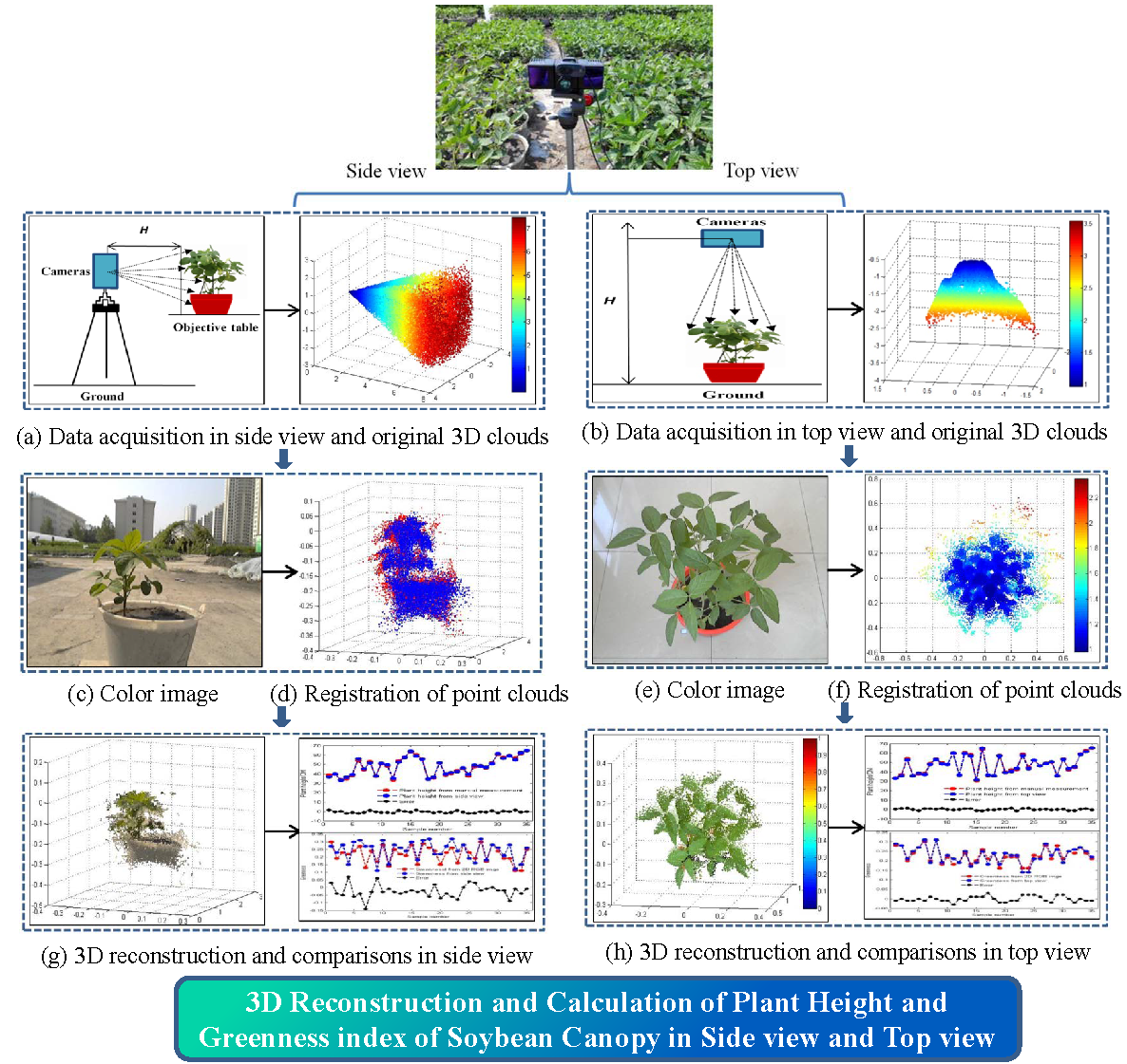
The overall processes and methods for performing a 3D reconstruction of the soybean canopy and the calculation of phenotypic traits are shown in Figure 1. First, raw 3D point cloud data including the soybean canopy information were captured from the side view (Figure 1a) and top view (Figure 1b), respectively, by using a multisource imaging system consisting of a photonic mixer detector (PMD; model: Camcube 3.0, PMDTech Company, Siegen, Germany) and an RGB camera (model: C270, Logitech Company, Lausanne, Switzerland). Second, the soybean canopies (Figure 1d,f) were extracted from the raw 3D cloud point data by executing the DBSCAN algorithm. Third, the RGB image and associated 3D point cloud information were fused together to reconstruct the geometric morphology of the soybean canopies (Figure 1g,h) by executing the PCA algorithm for a rough registration and the ICP algorithm for optimal registration between the input point cloud and reference point cloud. Last, phenotypic traits such as plant height and the greenness index were calculated. The phenotypic data of the soybean canopies were compared with the data collected by manual measurements, such that the accuracy of the developed system can be evaluated.
2.2. Experimental Treatments and Measurement of Phenotypic Traits
The plantation experiment was conducted in 2016 at the Heilongjiang Bayi Agricultural University. A total of 70 soybean plants, including four varieties (namely, Kennong23, Kennong29, Kennong30, and Kennong33), were cultivated in pots. The experiment was conducted in accordance with a randomized complete block design. Each variety was replicated 17 times and planted in a polyvinyl chloride (PVC) pot (25-cm diameter and 40-cm height) prior to disinfection and germination treatments of soybean seeds. Twenty kilograms of soil and sand (2:1 w/w) were mixed together and added to each pot. The nitrogen, phosphorus, and potassium nutrient compositions were 50 mg/kg, 30 mg/kg, and 30 mg/kg, respectively. One, two, or three soybean plants were grown in an individual pot. Plant height was measured with a ruler.
2.3. Multisource Imaging System
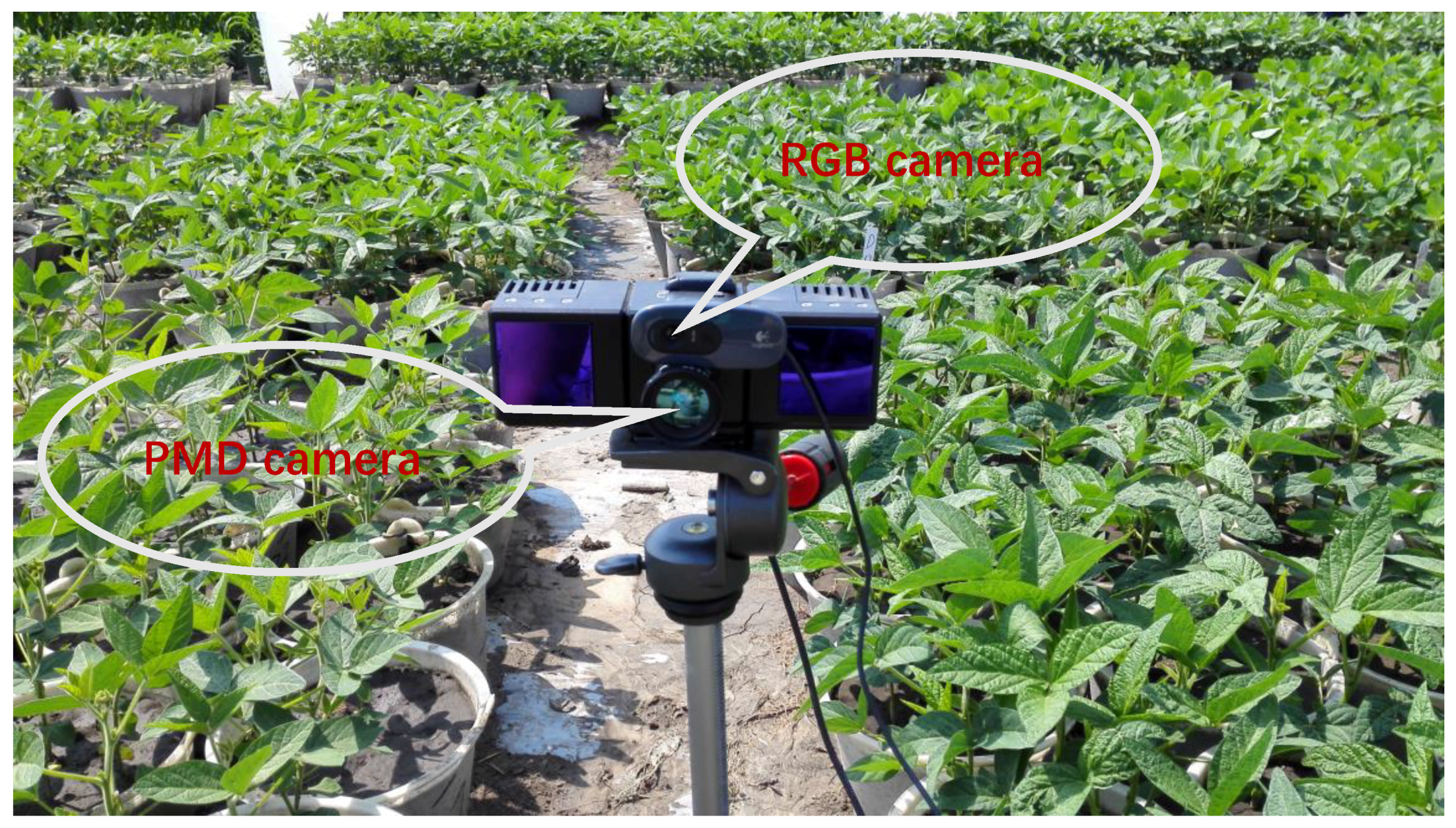
The multisource imaging system (Figure 2) was composed of a PMD camera and an RGB camera. The PMD is a developer of complementary metal oxide semiconductor (CMOS) 3D time-of-flight (TOF) components, and a provider of engineering support in the field of digital 3D imaging. With its active imaging system, this depth camera can irradiate an active light source onto objects. The light reflected from the objects is then used to generate the depth image by calculating the TOF between the emission and reception [11]. In addition to generating depth images, the PMD camera was used to construct three additional multisource images: an intensity image, an amplitude image, and a flag image. The intensity image was recorded to illustrate the average intensity of incident light, natural light, and near-infrared light mixed together, and the amplitude image was used to indicate the reflecting ability of the objects. The flag image reflected the quality of the image pixels. Although this imaging system has the powerful capability of acquiring multisource images, there is no color information therein. This deficiency can be overcome by using the spectral reflectance acquired from an RGB camera at a spatial resolution of 640 × 480 pixels. Moreover, the PMD camera can be operated at a high frame rate (40 frames/s), but a resolution thereof (200 × 200 pixels) is relatively low.
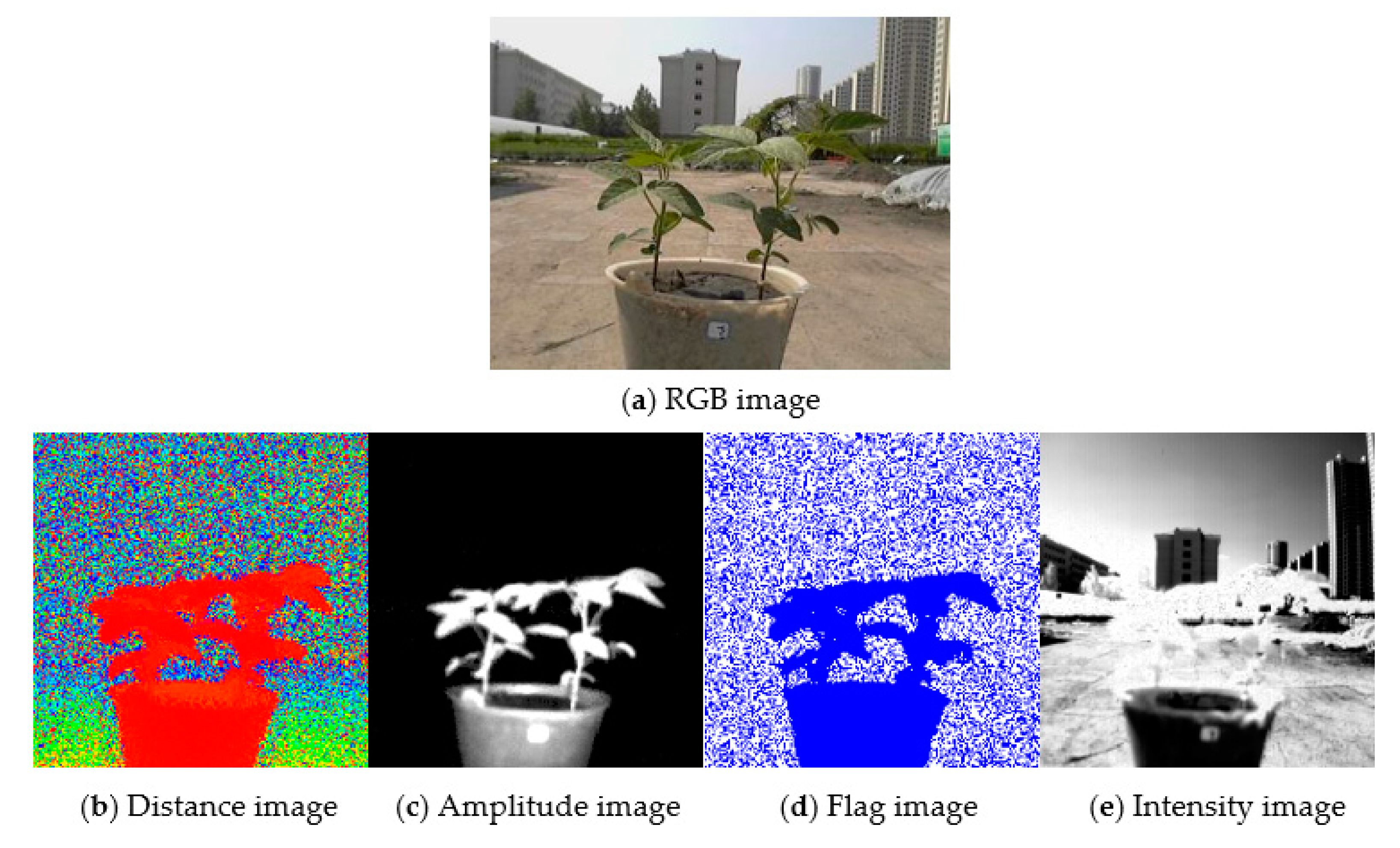
Figure 3 shows examples of the multisource images, including an RGB image, a distance image, an amplitude image, a flag image, and an intensity image. The multisource images played an important role in the 3D reconstruction of soybean canopies, and the RGB images provided rich color information of the 3D canopies. The distance images were used to generate accurate 3D distance information, including the information with respect to x, y, and z-axes. Additionally, the amplitude images aided in the removal of the background of the RGB images. The flag images could be used to verify the quality of the multisource images when the valid images were selected. Last, the intensity images and RGB images were used together to calibrate the binocular cameras via the manual selection of feature points. Therefore, the combination of these two cameras is advantageous for the 3D reconstruction of soybean canopies with color information therein. Figure 2 shows an integration of the RGB camera and the PMD camera. In this way, these two cameras (integrated as a multisource imaging system) could collect images simultaneously via the software preinstalled thereon.
2.4. Calibration of Multisource Imaging System
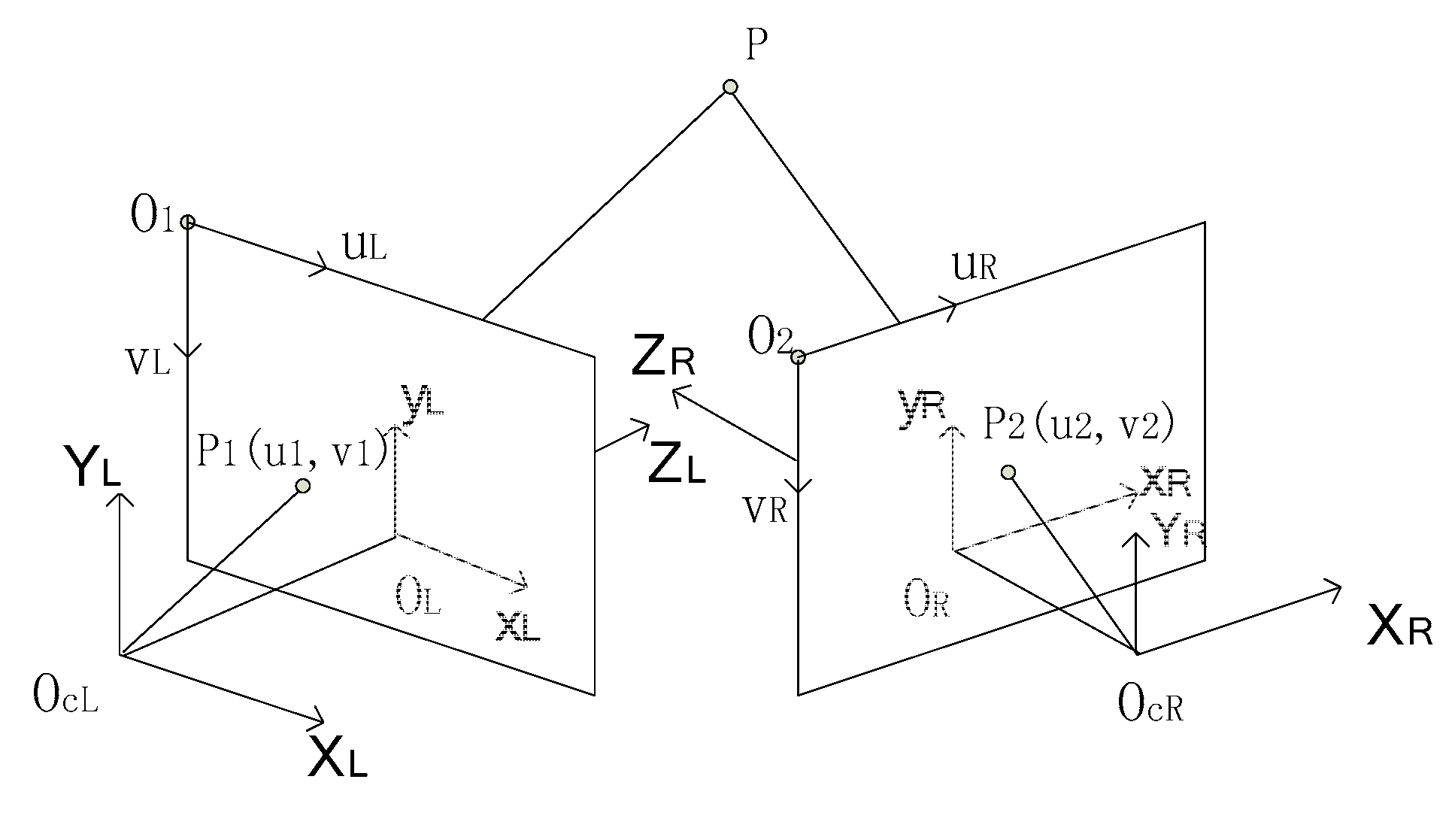
The multisource imaging system was a binocular vision system composed of a PMD camera and an RGB camera (Figure 4). The camera calibration toolbox of MATLAB (version: 8.2) was used to calibrate both cameras. The position of any point P in the space could be approximated as a pinhole imaging model. There were four coordinate systems (Figure 4): the camera coordinate system (OcL-XLYLZL and OcR-XRYRZR), the imaging plane coordinate system (OL-XLYL and OR-XRYR), the image coordinate system (O1-uLvL and O2-uRvR), and the world coordinate system.
The coordinates of P were (X1, Y1, Z1), (x1, y1), and (u1, v1) in the PMD camera’s coordinate system, imaging plane coordinate system, and image coordinate system, respectively. The coordinates of P were (X2, Y2, Z2), (x2, y2), and (u2, v2) in the RGB camera’s coordinate system, imaging plane coordinate system, and image coordinate system, respectively.
The relationship between the PMD and RGB coordinate systems is expressed by Equation (1):
where R is a 3 × 3 orthogonal matrix and T is a translation vector, which was the external parameter determined by the position of the cameras.
R and T are solved by using the calibration method provided by Zhou [23], and the final results of R and T are as follows:
The imaging system (the PMD and RGB cameras) achieved the optimal calibration effect via the optical calibration method mentioned above. However, due to the complexity of soybean canopies, we further calibrated the PMD and RGB cameras for fusion by using the registration method of image feature points based on the optical calibration method, so as to accurately reconstruct 3D soybean plants (Section 2.6.2).
2.5. Data Collection and RGB Image Preprocessing
The images were acquired by using the multisource imaging system between 10 am and 12 pm between 4–8 July 2016. The images were captured under natural environmental conditions at 28 °C and a light intensity of 1000 lux, and then stored in the laptop computer in a native raw format. Two shooting methods—namely, shooting from side view and shooting from top view—were compared based on an assessment of their ability to reflect plant height and greenness index. In addition, the effectiveness of 3D reconstruction by both methods was evaluated. Regardless of which method was used, when the images were collected, the whole plant or canopy had to be fitted within the field of view (FOV) of the cameras.
2.6. 3D Reconstruction
A three-step framework was proposed to reconstruct an individual soybean plant in the side view and top view. We compared the two data acquisition methods in terms of their ability to calculate two phenotypic traits. The comparison results were used to further evaluate the accuracy of the 3D reconstruction.
2.6.1. DBSCAN Algorithm for Point Cloud Filtering
We started with a raw point cloud without considering geometric and color information. Thus, the first important step in 3D reconstruction was to classify the useful points from the raw point clouds. We proposed extraction tasks with the DBSCAN [25] algorithm for side-view and top-view image acquisition methods (Figure 5). The information embedded in the raw data required for 3D reconstruction was not only reconstituted from the soybean plant, but also related to the background (building, sky, or people) within seven meters.
In this study, P was one set of 3D points in the raw data, and could be written as follows:
where , are the coordinates of , and r represents the real number set. NH represents the neighborhood of , which belongs to the following aggregate:
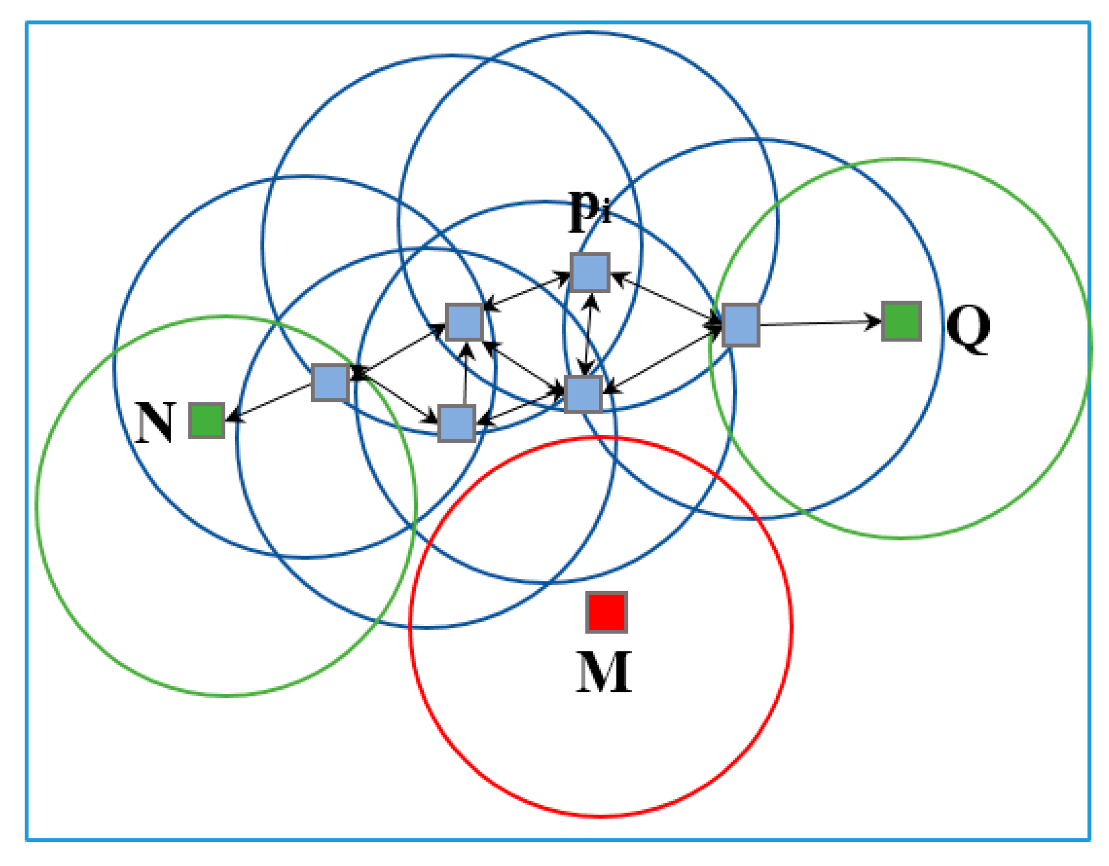
To apply DBSCAN clustering for the extraction of plant information, the raw points were divided into core points, (density) reachable points, and outliers, and are defined as follows: a core point must be within distance k (k was the maximum radius of the neighborhood from ); a point is reachable from if there is a path T1, …, Tn, with T1 = and Tn = Q, whereas each Ti + 1 is directly reachable from Ti; the outliers are the points that are not reachable from any other point. If was a core point, then it formed a cluster together with all of the points (core or non-core) that were reachable from it. Each cluster contained at least one core point; non-core points could be part of a cluster, but they formed its “edge” because they could not be used to reach additional points.
In Figure 6, minPts = 4. The point and the other blue points were core points, as the area surrounding these points in an NH radius contained at least four points (including the point itself); since they were all reachable from one another, they formed a single cluster. Points N and Q were not core points, but were reachable from Pi (via other core points); thus, points N and Q belonged to the cluster as well. Point M is a noise point that is neither a core point nor directly reachable.
For running DBSCAN, in addition to parameter k, a minimum number of points was needed to build a dense region, starting with a random point that had not been accessed before. A k-neighborhood of this starting point was then retrieved. In this research, if it contained at least 30 points within 0.06 m, a new cluster was generated. Otherwise, the point was marked as a noise point. If a point was a dense part of a cluster, then its k-neighborhood was also classified as that cluster. Hence, all of the points in the k-neighborhood were added to the cluster. This process continued until the density-connected cluster was thoroughly retrieved. All of the unvisited points were then traversed and processed for the purpose of detecting an additional cluster or noise point. After the DBSCAN algorithm was run, at least 32,690 points were filtered from the raw point cloud consisting of 200 × 200 points. Thus, 7310 effective points were extracted to form the 3D shape of a soybean plant.
2.6.2. Fusion of Multisource Images
The fusion of multisource images is a recent development and remains an active research field [26]. A major fusion problem concerning these multisource sensors resulted from the merging of a low-spatial resolution distance image and a high-spatial resolution RGB image. During this process, the PMD amplitude image and its corresponding RGB image were fused together to construct a 3D soybean plant containing color information. The whole procedure of this fusion involved coordinate selection, affine transformation, and the assignment of color information for 3D points.
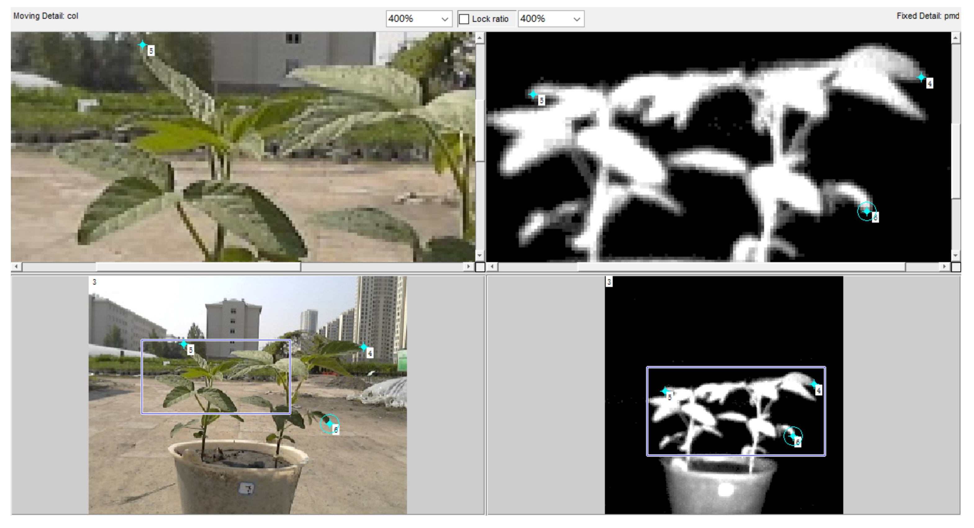
First, coordinate transformation was implemented based on the PMD camera coordinate system to generate two different coordinate systems that had uniform structures. A control point selection tool called cpselect (Figure 7) in the MATLAB (version: 8.2) environment was used to select three pairs of control points between the PMD amplitude image and its related RGB image, after which the coordinates of the control points were returned to a cpstruct structure.
After obtaining the cpstruct structure, the coordinate system of the RGB camera was transformed to that of the PMD camera via affine transformation, which is a linear mapping method that strongly preserves shapes for points, straight lines, and planes in an RGB image. Furthermore, to assign color information to its corresponding 3D point, a color index matrix was defined, which stored the corresponding relations between the coordinates of 3D points and the values of R, G, and B channels. After the images were fused, a new distance image with color information was constructed in a 3D coordinate system. In the resultant RGB image, the size was changed to 200 × 200 pixels, which was a one-to-one match with its original distance image according to the color index matrix.
2.6.3. Registration of 3D Point Clouds between Front and Back Sides
The whole canopy image could be obtained simultaneously by cameras in the top view. As such, the multisource images acquired in the top view were not subjected to image registration between two sides (front and back), while this process was needed for those images collected in the side view. In this study, to show the 3D reconstruction of a soybean plant in the side view, the images acquired from both sides (front and back) of the plant were processed by registering the 3D point clouds.
In this research, was the aggregate of the point clouds, ; represents the center of a point cloud, ; the variance was ; and the covariance matrix was .
For the input point cloud and the reference point cloud , the purpose of the registration was to determine the optimum similarity transformation and apply this transformation on , which transformed the coordinate of to the counterpart of .
where R, t, and s are the rotation matrix, translation vector, and scale factor, respectively.
The ICP, which is an algorithm [27] that is capable of maximally reducing the difference between the two point clouds, was used to perform the two abovementioned processes of point cloud registration. Many variants of ICP, which has been widely used for the geometric alignment of 3D surfaces generated by various scan methods, have been developed. The two most popular variants are point-to-point and point-to-projection algorithms. The former performs better at registration tasks primarily because the PCA algorithm [28] is applied in advance to obtain a rough registration of the two components of the point clouds. This work was achieved by the combination of the PCA and ICP algorithms. R and t of Equation (4) could ultimately be solved by the singular value decomposition (SVD) of the ICP algorithm.
(1) PCA for rough registration
The PCA algorithm was applied to determine the principal axis direction between and , and the rough registration results were used as inputs for the ICP algorithm for exact registration by the ICP algorithm. The processes were as follows:
First, the point cloud was decomposed by SVD, from which the left singular vector U, eigenvalue matrix D, and right singular vector V could be obtained at the same time. The SVD operation for was calculated by Equation (2):
Second, the PCA coordinate was established, and the direction of axis was determined by and . Afterward, a similarity transformation was calculated by Equation (6), during which was transformed from the original coordinate to the PCA coordinate.
There were four candidate transformations because of the uncertainty of the principal axis direction. Thus, the optimal transformation must be selected from four transformations, which could minimize the registration error and maximize the normal vector consistency for and .
The PCA algorithm ultimately achieved basic registration between the input and reference point clouds via rotation, translation, and zoom operations. The basic registration result was subsequently used as an input for the ICP algorithm.
(2) ICP for optimal registration
We defined P and Q as having the same points, although they were from two point cloud aggregates ( and , respectively). The coordinates of P and Q were and ; any point in aggregate could be expressed by . Thus, the Euclidean distance between P and was then calculated by the following:
Essentially, the steps of the ICP algorithm for optimal registration are described as follows:
First, we obtained the source point cloud and the reference point cloud .
Second, we searched the nearest point in input point cloud for any point in reference point cloud using Formula (7), which could best align each source point to its match after weighting and rejecting outlier points.
Next, we solved the rotation transform matrix , the translation vector t and the deviation via SVD in accordance with Equations (9) to (15). In addition, Equation (8) served as the objective function with the minimum square error [29].
Further, we transformed the source points using the obtained transformation in the previous step to obtain .
We then analyzed whether the deviation was convergent or not. If it was, the final matrix of the coordinate transformation and were determined; otherwise, it was iterated from step 2 until was a convergence. The similarity transformation could be obtained after the convergence of .
The final transformation matrix T from to was as follows:
When the algorithms above were integrated together, the 3D shape of the soybean plant was reconstructed by registering the two point clouds acquired from the front and back. Traditionally, missing data due to occlusions and misarranged 3D point positions are calibrated by hole-filling algorithms according to the curvature of the surrounding triangle mesh [30]. Although an entire 3D model could be built in accordance with this method, it was not applicable for reconstruction with color information primarily because the values of the R, G, and B channels of the point generated by the hole-filling algorithms could not represent the real spectral reflectance of soybean canopies. Therefore, the next step for phenotyping analysis was based on the 3D plant model built without hole-filing algorithms applied.
2.7. Methods of Calculating 3D Phenotypic Traits
Referring to the current 3D reconstruction approaches for soybean plants, we used a mathematical method to describe plant organs, aiming at simplifying data processing and providing a repeatable and objective parameterization of growth processes. We simulated relevant plant phenotypic traits such as plant height and canopy greenness index in the side view and top view separately. These traits are important parameters for evaluating plant quality, as they play an important role in the entire growth stage via photosynthesis. A total of 70 soybean plants (35 plants for the side view and 35 plants for the top view) were selected from the field for measuring these two traits.
2.7.1. Method of Calculating Plant Height
Plant height is defined as the shortest distance from the upper boundary of the main photosynthetic tissues (excluding inflorescences) on a plant to the ground level [31,32], expressed in meters. Among various phenotypes, plant height is an important geometric parameter; it can be used not only as an indicator of whole soybean growth, but also to quantify other advanced parameters such as yield and total biomass [33,34]. Soybean plant height is a particularly important factor used by breeders for screening and selecting improved varieties.
Plant height is traditionally measured manually with rulers or handheld devices such as laser rangefinders. However, these methods are time-consuming and labor-intensive, and thus are not applicable for large-scale phenotyping analysis. Advances in 3D imaging techniques allow the measurement of geometric traits such as plant height via the acquisition of accurate and efficient data concerning the 3D structures of plants.
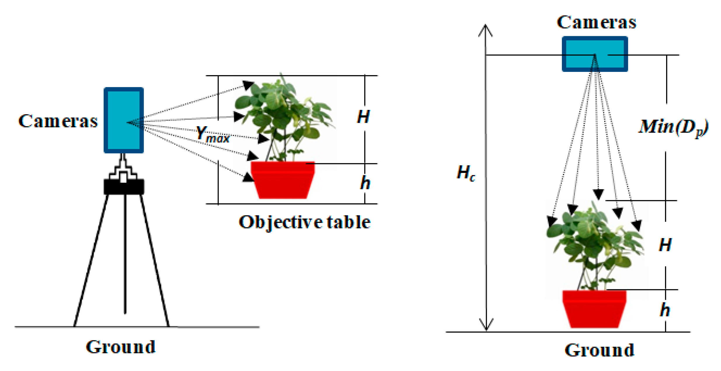
For top-view depth images, the camera was installed on a tripod that had an adjustable height, and each plant was placed on the ground in the center of the camera’s FOV. According to the TOF principle, the pixel intensity reflected the distance between objects and the lens of the camera in millimeters. A pixel would be invalid if its intensity was zero because of no reflection from an object. According to Figure 5(right), soybean plant height was calculated via Equation (17) in the 3D space of the soybean reconstruction model.
where represents the height of the soybean plant in millimeters and is the distance from the lens of the camera to the ground level in millimeters; was 2000 mm when the images were captured via the top view-based method. To capture the whole canopy image, an adjusted value was used according to the actual plant height. In addition, in this equation, , , , and indicate the pot height shown in the image, the pixel set in a distance image, one pixel in the pixel set , and the distance value of pixel , respectively. Consequently, a total of 35 plant height measurements were made for calculating the relative error between the 3D measurements and manual measurements.
Moreover, for the side-view depth images, plant height was derived as follows:
where and have the same meaning as above, and is the maximum value of the coordinate of the depth image. Further, the height of 35 plants was subjected to correlation analysis with the manual measurements.
2.7.2. Method of Calculating Greenness Index
The greenness index is a primary phenotypic trait concerning the color characteristic of the leaf, which can be used for the classification of plant health status [35] and the inversion of both the nitrogen content and chlorophyll content [19]. Conventionally, visual inspection and chemical analysis have been the major methods used for the evaluation of plant health. Methods involving leaf color charts (LCCs) are widespread among farmers, but much subjectivity is involved in the results. The chemical analysis-based approach is destructive and not conducive to continuous plant growth. The image color indices in RGB color space can serve as a more objective yet nondestructive method for plant health assessment [36].
In this study, the values of the R, G, and B channels of each point cloud were extracted from the 3D plant canopy. The invalid points and object colors were omitted from the calculation according to the distance value of the objects if they were not derived from the canopy. All of the points of the 3D point cloud were traversed to extract their values of the R, G, and B channels for the purpose of calculating the greenness index.
An original input 3D image with color information was investigated in the RGB color space. The imaging effect therein was subjected to a white balance treatment [17] that was processed in its corresponding 2D image prior to the RGB decomposition in which the R, G, and B channels of the image were extracted for determining the greenness index. We applied the following scheme to obtain the greenness index, which was used to quantify the relative health of the leaves [16]:
where GS is the greenness index and and represented the values of the , and channels at coordinates respectively. Consequently, 35 values of canopy greenness from the side view and 35 values of canopy greenness from the top view were compared with those obtained manually. The manual measurement values of canopy greenness index were calculated via the following method: all of the 2D images of the soybean canopies acquired by the RGB camera of the multisource imaging system were extracted from their complex background, and the average values of the R, G, and B channels of the whole canopy image were calculated separately by Adobe Photoshop software (version: CS6). The manually measured greenness values of greenness were determined according to Equation (19).
3. Results
3.1. 3D Reconstruction
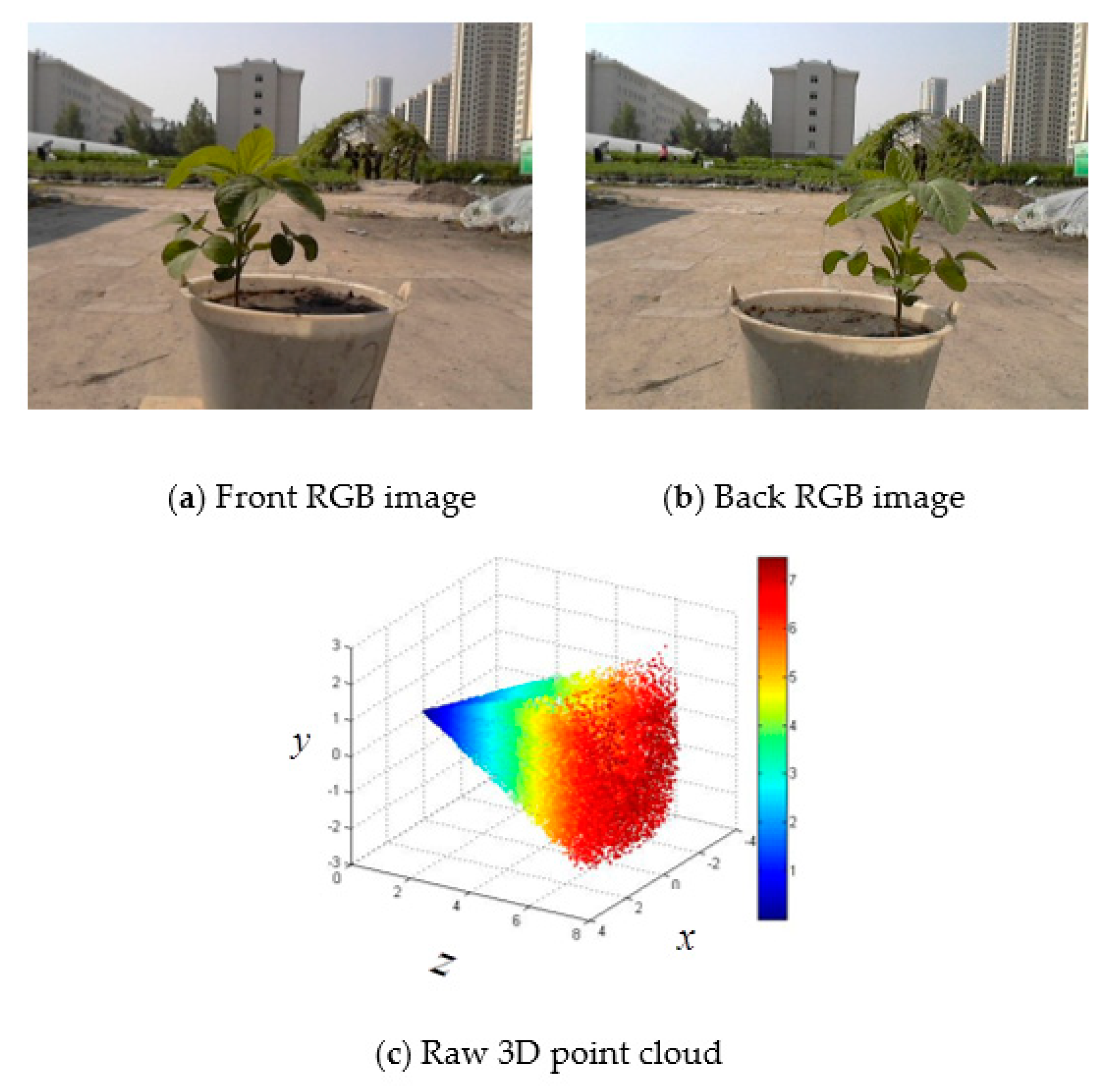
For illustration purposes in this paper, a single plant and multiple plants were selected as typical examples for showing the reconstruction results. Soybean plants studied via two different acquisition methods (side view and top view) can be distinguished by the color of their pots. During data collection, the multisource imaging system was placed 80 cm from the target potted soybean plants; the positions were not changed. Thus, each pot was rotated 180 degrees around the center of the pot to acquire the back images after obtaining the front images of a soybean plant.
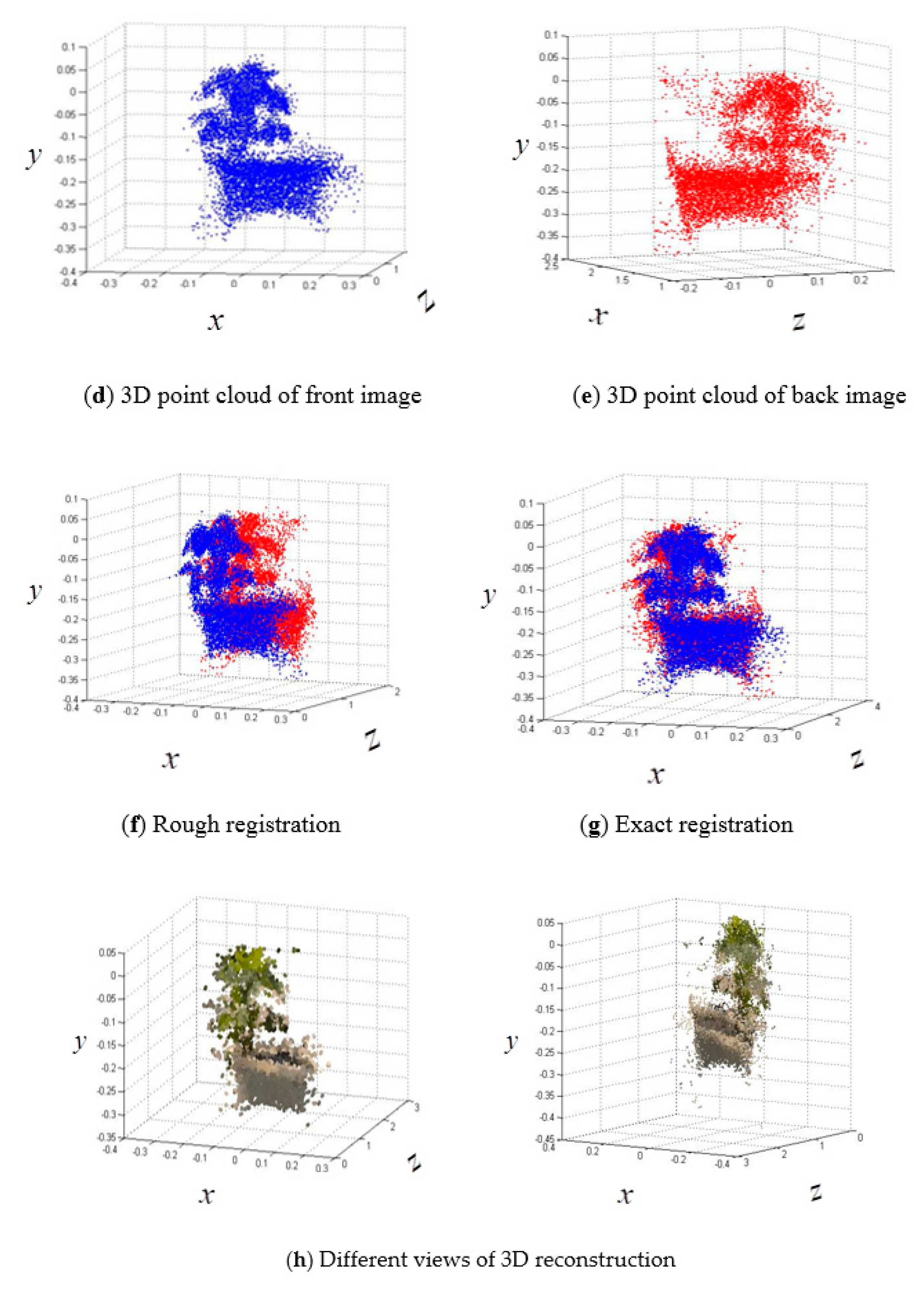
For the side view, the target 3D points (Figure 8d,e) from the front and back sides were extracted from the complex background (Figure 8c) via the DBSCAN algorithm mentioned in Section 2.6.1, and were then fused with color information according to the corresponding control points between the RGB image and amplitude image. Figure 8f,g illustrates the rough registration and exact registration results via PCA and ICP algorithms, respectively. Final reconstruction results for a single plant are shown in Figure 8h, which demonstrates that the entire shape with color information was reconstructed well, although some scattered 3D points were not fully clustered. Moreover, the accuracy of correspondence between RGB and 3D coordinates needs to be improved further.
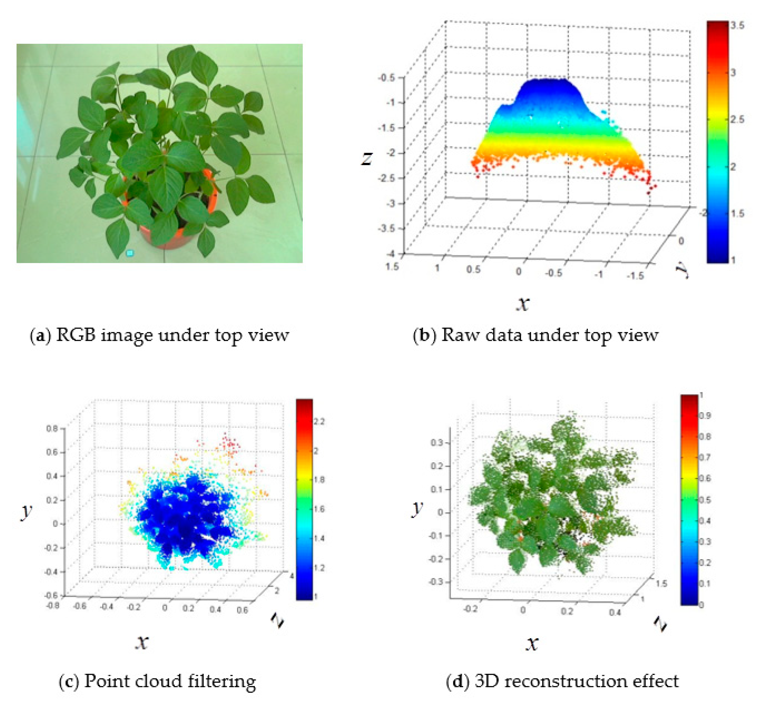
Although many more phenotypic traits such as stem diameter and leaf angle can be researched via the 3D reconstruction of a soybean plant in the side view compared with the top view, relatively complex and time-consuming algorithms such as DBSCAN and registration algorithms were used to reconstruct the 3D shape of soybean canopies. Thus, for the two phenotypic traits (plant height and greenness index) in this paper, the much simpler top-view acquisition method was used to extract information on plant height and greenness index; this information was not subjected to image registration between the front and back of the soybean canopies. In addition, for the purpose of avoiding the effects of wind, the plants were moved indoors for acquiring images from the top view. Similarly, the canopy images were segmented from the raw data (Figure 9b) based on the DBSCAN algorithm combined with distance thresholding (TH = 80 mm) to remove any miscellaneous points. Notably, the thresholding needed to be adjusted according to the height of the plants. The canopy depth and plant height indicated by color bar in Figure 9c were calculated by Equation (17), and the 3D canopy was ultimately reconstructed by the fusion of the distance image and the two-dimensional (2D) RGB image. As shown in Figure 9d, the pixels at the edge of the leaves were missing because of the weak reflection at the edges. In addition, some useless red pixels, which were part of the pot, were observed in the final reconstruction. This phenomenon occurred mainly because a few leaves covered some sections of the pot, which affected the threshold setting. However, these red pixels did not affect the greenness calculations, and did not negatively impact the plant height measurements.
The resolution of the 3D reconstruction of soybean plants is 200 × 200 pixels not only for the side view, but also for the top view. Each pixel pitch is 45 μm, which depended on the resolution of the PMD camera.
3.2. Accuracy of Plant Height Measurements in the Side and Top Views
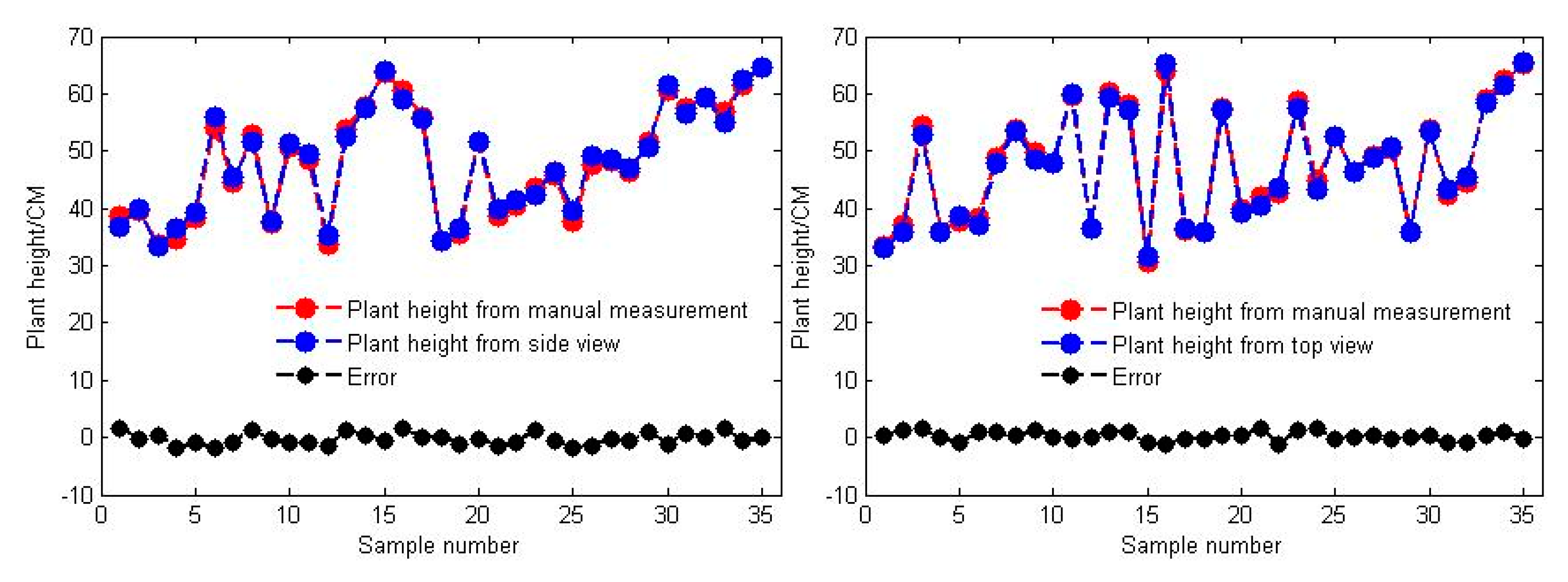
The plant height data obtained from the side view-based and top view-based 3D reconstructions were compared with the manually measured data (Figure 10). The plant height was measured via the algorithm described in Section 2.7.1. The linear best-fit models comparing the side view-based and top view-based plant height measurements with the manual measurements yielded determination coefficient (R2) values of 0.9890 and 0.9936, respectively. However, there were some biases: the side view-based plant heights fluctuated to some degree (by −1.8 cm to 1.7 cm), and the top view-based errors in the plant height calculations ranged from −1.1 cm to 1.5 cm. The average error for the side view and top view was 0.6713 cm and 0.2600 cm, respectively.
The 3D measurements indicated that the multisource imaging system could measure soybean plant height with a high degree of accuracy under both natural light conditions and indoor conditions. These findings provided useful guidelines for soybean plant height measurements under field conditions. Plant height phenotypes could be applied to guide the screening of soybean genotypes. For example, plant height is an indicator of early maturing soybean cultivars, which could reduce yield losses due to pests and diseases. Additionally, plant height can also be used to predict leaf area index and yield.
3.3. Accuracy of Greenness in the Side and Top Views
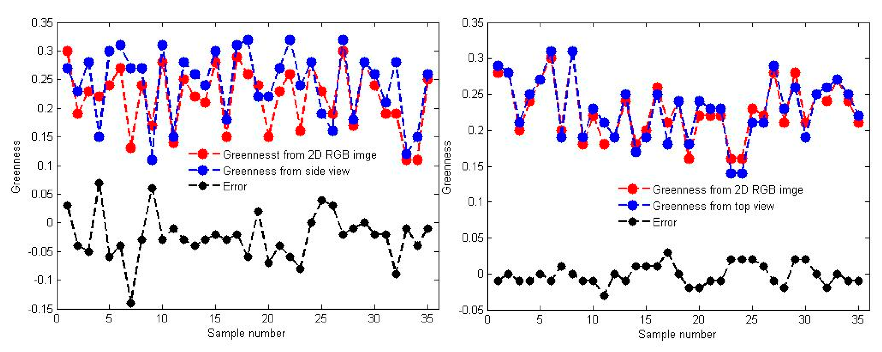
A crucial focus of this study was to produce a practical method for determining the greenness index, which provides valuable data to crop experts for diagnosing the diseases and nutrient conditions of soybean plants. The greenness index was calculated using the procedure described in Section 2.6.2. Figure 11 shows a comparison of the results of the 3D measurements and manual measurements. The greenness index was highly correlated with that assessed manually (R2 of 0.8864 and an average error of 0.0117) for top view-based data; the minimum and maximum deviations were −0.03 and 0.03, respectively. The side view-based measurements yielded a correlation of R2 = 0.6059, with an average error of 0.0386, and the deviation of calculation fluctuated between −0.14 and 0.07.
Although the top view-based plant height and greenness measurements were more accurate than their side view-based counterparts, other phenotypic traits such as leaf angle, branch angle, and stem diameter could not be measured effectively from the top view. Consequently, we performed 3D soybean reconstructions in the side view. The above-mentioned phenotypic traits will be considered in our future research. Furthermore, side-view 3D reconstruction will be improved by considering weather factors during data collection.
4. Discussion
4.1. Analysis of Experimental Results
In this paper, algorithms of the 3D reconstruction of soybean canopies were proposed for use in phenotyping analysis based on two acquisition methods (side view and top view). Additionally, plant height and greenness index were calculated.
In terms of accuracy, there was no significant difference in plant height between the side view and top view; the R2 values from the side view and top view were 0.9890 and 0.9936, respectively. However, the side view-based greenness was less accurate than its top-view counterpart because of the random environmental factors under the natural light conditions affecting the 3D reconstructions of soybean canopies. The R2 values from the side view and top view were 0.6059 and 0.8864, respectively.
Although the present experimental results meet the requirements for calculating the plant height and greenness index of soybean canopies, some aspects should be considered for obtaining more accurate greenness index data in the side view under natural conditions. The first aspect involves environmental factors, especially weather conditions. The ideal weather conditions involve a sunny day with no wind. However, the actual environmental conditions, such as high winds or rainy weather, cannot be controlled, but can be avoided. The second aspect involves the algorithms; both the DBSCAN and registration algorithms should be improved to acquire the optimal 3D reconstruction results of soybean canopies. The use of a modified DBSCAN algorithm [37] to cluster a 3D point cloud for extracting soybean canopies from complex backgrounds will be studied. In addition, compared with classic algorithms, improved ICP algorithms [38] can be used for more accurate and efficient exact registration between two pieces of 3D point clouds.
4.2. Evaluation of Algorithm Robustness
Robustness is a key indicator in algorithm evaluation. The algorithms in this research met the requirements needed for the 3D reconstruction and phenotyping analysis of soybean plants. The robustness of the algorithms could be evaluated from the aspects described below.
First, it is well known that light intensity will impact imaging. Therefore, to prove the applicability of the algorithms for 3D reconstruction, the multisource images were acquired both indoors and under natural conditions. Image acquisition under natural light was performed between 10 am and 12 pm, and the maximum light intensity reached 1000 lux. Under these circumstances, the algorithms worked well for the 3D reconstruction of soybean canopies.
Moreover, wind is another factor that affects 3D reconstruction. The presence of wind during data collection might result in the vibration or color distortion of the canopy, leading to inaccurate fusion between the 3D points and the RGB image. Some results proved that there was obvious image distortion at the edges and thickness of leaf organs when the wind speed varied from 0.9 m/s to 2.4 m/s. Therefore, to improve the stability of the algorithms, weather conditions with no or low wind (less than 2.4 m/s) are the best environments in which to obtain optimal 3D reconstructions of soybean canopies for phenotyping analysis [39,40].
In addition, background complexity is the third factor that affects imaging. During image acquisition, the background consisted of buildings, plants, sky, and ground, which could be considered a complex environment (Figure 3a). Furthermore, we acquired images under the conditions indicated above (sunny day, gentle breeze, and complex background).
Our correlation results yielded an R2 value of 0.9890 for plant height and an R2 value of 0.6059 for the greenness index under natural light conditions, both of which could be used to evaluate 3D reconstruction results. In addition, these experimental results, which were based on existing soybean samples, were accurate. Thus, the algorithms proposed in this paper exhibited excellent robustness for plant phenotyping analysis.
4.3. Advantages of Multisource Imaging Systems
This study has shown the capability of using both the fusion of PMD and RGB camera images and the proposed algorithm to measure the plant height and greenness index of soybean canopies rapidly and accurately. From plant science and breeding perspectives, the plant height trait could be used for selecting soybean genotypes. For example, plant height is used as an indicator of early maturing plant cultivars [41,42] to avoid yield losses that result from diseases and insect–pest complexes. In addition, measuring the greenness index over time at every growth stage could be used to indicate the effectiveness of plant energy consumption, which can be potentially used for the diagnosis of nutrient deficiencies. From a technical perspective, plant height and greenness can also be accurately measured with other imaging sensors such as light detection and ranging (LiDAR) [43] and more accurate RGB cameras in hue, saturation, and intensity (HSI) or hue, saturation, and value (HSV) color spaces [44], respectively. The use of PMDs to reconstruct the 3D geometry of plants has been explored, and the results of the present study demonstrated that a PMD camera operating in tandem with an RGB camera can provide accurate measurements of plant height and greenness, which creates new opportunities for field-based soybean plant phenotyping.
4.4. Future Work
In the present framework of phenotyping, plants are usually monitored one after another with noninvasive measurement devices. As an initial proof of feasibility, we have studied soybean plants cultivated in pots. However, a promising strategy could be developed to increase the throughput at larger observation scales by capturing multiple soybean plants in a single image. Additionally, under field conditions, the spatial arrangement of soybean plants is less regular than that in well-controlled environments. Thus, it is challenging to quantify the effects of crop spatial arrangement.
In addition, both views (side view and top view) are important for phenotyping analysis. Plant height, the leaf area index, and the greenness index can be measured accurately from the top view, but this view is not suitable for measuring other phenotypic traits such as leaf angle, branch angle, and stem diameter, which can be calculated effectively from the side view. Thus, future work will focus on improving the algorithms for 3D reconstruction from not only the side view but also the top view to acquire additional elaborate phenotypic traits. Notably, environmental factors—especially weather conditions—should be considered when data are collected in natural environments. Sunny days with low wind are considered the best conditions for phenotyping analysis.
5. Conclusions
In this paper, we developed a streamlined method to measure the specific phenotypic traits of soybean plants based on a 3D reconstruction containing color information. The main achievements are summarized as follows:
- (1)
- An active imaging system consisting of a PMD camera and an RGB camera was used to collect multi-images of soybean plants. First, the DBSCAN algorithm was used to extract soybean plant information from the complex raw dataset. Next, the multisource images were fused together for the purpose of constructing 3D images that contain color information. Last, 3D points from the front and back sides were registered using the ICP algorithm. The proposed methodology can be used to reconstruct a 3D soybean plant for a phenotyping analysis that includes measurements of plant height and greenness.
- (2)
- By combining this multisource imaging system and the proposed algorithms, we can accurately measure soybean plant height. Correlation analysis between the estimated and manual measurements yielded R2 values of 0.9890 and 0.9936 for the side view and top view, respectively, and their average errors were 0.6713 cm and 0.2600 cm, respectively. From a plant breeding perspective, this finding could be especially useful for rapidly predetecting a subset of soybean genotypes that are of suitable height for expected yields and machine harvesting.
- (3)
- Compared with the side view-based greenness, the top view-based greenness was much more accurate. The greenness index estimated from the top view-based data was highly correlated with the manually assessed greenness index: the R2 value was 0.8864, and the average error was 0.0117. However, the R2 value decreased to 0.6059 (average error of 0.0386) for the side view-based results. This result was primarily due to the impact of the natural environment, such as wind and sunlight, which led to some fusion and registration deviations between the 3D points and their corresponding RGB images. The algorithm itself needs to be improved.
Author Contributions
H.G. and S.Y. conceived and designed the experiments; M.L. performed the experiments and acquired the 3D data of soybean canopy; X.M., H.G. and M.L. analyzed and process the data; H.G. and X.M. wrote the paper.
Funding
This study was funded jointly by National Natural Science Foundation of China (31601220), Natural Science Foundation of Heilongjiang Province (QC2016031), China Postdoctoral Science Foundation (2016M601464, 2016M591559), and Support Program for Natural Science Talent of Heilongjiang Bayi Agricultural University (ZRCQC201806).
Acknowledgments
The authors would like to thank the three anonymous reviewers, academic editors, Gang Liu, Minzan Li and Yajing Zhang for their precious suggestions that significantly improved the manuscript.
Conflicts of Interest
The authors declare no conflict of interest.
References
- Li, L.; Zhang, Q.; Huang, D. A review of imaging techniques for plant phenotyping. Sensors 2014, 14, 20078–20111. [Google Scholar] [CrossRef] [PubMed]
- Phillips, R.L. Mobilizing science to break yield barriers. Crop Sci. 2010, 50 (Suppl. 1), S-99–S-108. [Google Scholar] [CrossRef]
- Houle, D.; Govindaraju, D.R.; Omholt, S. Phenomics: The next challenge. Nat. Rev. Genet. 2010, 11, 855. [Google Scholar] [CrossRef] [PubMed]
- Dhondt, S.; Wuyts, N.; Inzé, D. Cell to whole-plant phenotyping: The best is yet to come. Trends Plant Sci. 2013, 18, 428–439. [Google Scholar] [CrossRef] [PubMed]
- Fiorani, F.; Schurr, U. Future scenarios for plant phenotyping. Annu. Rev. Plant Biol. 2013, 64, 267–291. [Google Scholar] [CrossRef] [PubMed]
- Minervini, M.; Scharr, H.; Tsaftaris, S.A. Image analysis: The new bottleneck in plant phenotyping. IEEE Signal Process. Mag. 2015, 32, 126–131. [Google Scholar] [CrossRef]
- Furbank, R.T.; Tester, M. Phenomics–technologies to relieve the phenotyping bottleneck. Trends Plant Sci. 2011, 166, 35–644. [Google Scholar] [CrossRef] [PubMed]
- Golbach, F.; Kootstra, G.; Damjanovic, S.; Otten, G.; van de Zedde, R. Validation of plant part measurements using a 3D reconstruction method suitable for high-throughput seedling phenotyping. Mach. Vis. Appl. 2016, 27, 663–680. [Google Scholar] [CrossRef]
- Haughton, A.J.; Bohan, D.A.; Clark, S.J.; Mallott, M.D.; Mallott, V.; Sage, R.; Karp, A. Dedicated biomass crops can enhance biodiversity in the arable landscape. GCB Bioenergy 2016, 8, 1071–1081. [Google Scholar] [CrossRef] [PubMed]
- Chaudhury, A.; Ward, C.; Talasaz, A.; Ivanov, A.G.; Brophy, M.; Grodzinski, B.; Huner, N.P.A.; Patel, R.V.; Barron, J.L. Machine Vision System for 3D Plant Phenotyping. arXiv 2017, arXiv:1705.00540. [Google Scholar]
- Chéné, Y.; Rousseau, D.; Lucidarme, P.; Bertheloot, J.; Caffier, V.; Morel, P.; Belin, É.; Chapeau-Blondeau, F. On the use of depth camera for 3D phenotyping of entire plants. Comput. Electron. Agric. 2012, 82, 122–127. [Google Scholar] [CrossRef] [Green Version]
- Ruiz-Altisent, M.; Ruiz-Garcia, L.; Moreda, G.P.; Lu, R.; Hernandez-Sanchez, N.; Correa, E.C.; Diezma, B.; Nicolaï, B.; García-Ramos, J. Sensors for product characterization and quality of specialty crops—A review. Comput. Electron. Agric. 2010, 74, 176–194. [Google Scholar] [CrossRef] [Green Version]
- Paulus, S.; Behmann, J.; Mahlein, A.K.; Plümer, L.; Kuhlmann, H. Low-cost 3D systems: Suitable tools for plant phenotyping. Sensors 2014, 14, 3001–3018. [Google Scholar] [CrossRef] [PubMed]
- Pound, M.P.; French, A.P.; Murchie, E.H.; Pridmore, T.P. Automated recovery of three-dimensional models of plant shoots from multiple color images. Plant Physiol. 2014, 166, 1688–1698. [Google Scholar] [CrossRef] [PubMed]
- Wang, Y.; Wang, D.; Shi, P.; Omasa, K. Estimating rice chlorophyll content and leaf nitrogen concentration with a digital still color camera under natural light. Plant Methods 2014, 10, 36. [Google Scholar] [CrossRef] [PubMed] [Green Version]
- Guan, H.; Li, J.; Ma, X. Recognition of soybean nutrient deficiency based on color characteristics of canopy. J. Northwest A F Univ. 2016, 44, 136–142. [Google Scholar]
- Cheng, H.; Shi, Z.X.; Li, J.T.; Pang, L.X.; Feng, J. A color correction method based on standard white board. J. Agric. Univ. Heibei 2007, 30, 105–109. [Google Scholar]
- Pan, B.; Liang, S. Estimation of chlorophyll content in apple tree canopy based on hyperspectral parameters. Spectrosc. Spectr. Anal. 2013, 33, 2203–2206. [Google Scholar]
- Baresel, J.P.; Rischbeck, P.; Hu, Y.; Kipp, S.; Barmeier, G.; Mistele, B.; Schmidhalter, U. Use of a digital camera as alternative method for non-destructive detection of the leaf chlorophyll content and the nitrogen nutrition status in wheat. Comput. Electron. Agric. 2017, 140, 25–33. [Google Scholar] [CrossRef]
- Hu, Y.; Wang, L.; Xiang, L.; Wu, Q.; Jiang, H. Automatic non-destructive growth measurement of leafy vegetables based on kinect. Sensors 2018, 18, 806. [Google Scholar] [CrossRef] [PubMed]
- Bai, G.; Ge, Y.; Hussain, W.; Baenziger, P.S.; Graef, G. A multi-sensor system for high throughput field phenotyping in soybean and wheat breeding. Comput. Electron. Agric. 2016, 128, 181–192. [Google Scholar] [CrossRef]
- Araus, J.L.; Cairns, J.E. Field high-throughput phenotyping: The new crop breeding frontier. Trends Plant Sci. 2014, 19, 52–61. [Google Scholar] [CrossRef] [PubMed]
- Zhou, W.; Liu, G.; Ma, X.; Feng, J. Study on multi-image registration of apple tree at different growth stages. Acta Opt. Sin. 2014, 34, 0215001. [Google Scholar] [CrossRef]
- Naik, H.S.; Zhang, J.; Lofquist, A.; Assefa, T.; Sarkar, S.; Ackerman, D.; Singh, A.; Singh, A.K.; Ganapathysubramanian, B. A real-time phenotyping framework using machine learning for plant stress severity rating in soybean. Plant Methods 2017, 13, 23. [Google Scholar] [CrossRef] [PubMed]
- Parimala, M.; Lopez, D.; Senthilkumar, N.C. A survey on density based clustering algorithms for mining large spatial databases. Int. J. Adv. Sci. Technol. 2011, 31, 59–66. [Google Scholar]
- Li, S.; Kang, X.; Fang, L.; Hu, J.; Yin, H. Pixel-level image fusion: A survey of the state of the art. Inf. Fusion 2017, 33, 100–112. [Google Scholar] [CrossRef]
- Glira, P.; Pfeifer, N.; Briese, C.; Ressl, C. Rigorous strip adjustment of airborne laserscanning data based on the ICP algorithm. ISPRS Ann. Photogramm. Remote Sens. Spat. Inf. Sci. 2015, 2, 73–80. [Google Scholar] [CrossRef]
- Deshpande, N.T.; Ravishankar, S. Face Detection and recognition using Viola-Jones algorithm and fusion of PCA and ANN. Adv. Comput. Sci. Technol. 2017, 10, 1173–1189. [Google Scholar]
- Chen, B.; Deng, L.; Duan, Y.; Chen, A.; Zhou, J. Multiple model fusion in 3D reconstruction: Illumination and scale invariance. J. Tsinghua Univ. 2016, 56, 969–973. [Google Scholar]
- Paulus, S.; Schumann, H.; Kuhlmann, H.; Léon, J. High-precision laser scanning system for capturing 3D plant architecture and analysing growth of cereal plants. Biosyst. Eng. 2014, 121, 1–11. [Google Scholar] [CrossRef]
- Peìrez-Harguindeguy, N.; Díaz, S.; Garnier, E.; Lavorel, S.; Poorter, H.; Jaureguiberry, P. New handbook for standardised measurement of plant functional traits worldwide. Aust. J. Bot. 2013, 61, 167–234. [Google Scholar] [CrossRef] [Green Version]
- Jiang, Y.; Li, C.; Paterson, A.H. High throughput phenotyping of cotton plant height using depth images under field conditions. Comput. Electron. Agric. 2016, 130, 57–68. [Google Scholar] [CrossRef]
- Demir, N.; Sönmez, N.K.; Akar, T.; Ünal, S. Automated measurement of plant height of wheat genotypes using a DSM derived from UAV imagery. Multidiscip. Digit. Publ. Inst. Proc. 2018, 2, 350. [Google Scholar] [CrossRef]
- Zotz, G.; Hietz, P.; Schmidt, G. Small plants, large plants: The importance of plant size for the physiological ecology of vascular epiphytes. J. Exp. Bot. 2001, 52, 2051–2056. [Google Scholar] [CrossRef] [PubMed]
- De Ocampoa, A.L.P.; Albob, J.B.; de Ocampoc, K.J. Image analysis of foliar greenness for quantifying relative plant health. Ed. Board 2015, 1, 27–31. [Google Scholar]
- Kurc, S.A.; Benton, L.M. Digital image-derived greenness links deep soil moisture to carbon uptake in a creosotebush-dominated shrubland. J. Arid Environ. 2010, 74, 585–594. [Google Scholar] [CrossRef]
- Ienco, D.; Bordogna, G. Fuzzy extensions of the DBScan clustering algorithm. Soft Comput. 2018, 22, 1719–1730. [Google Scholar] [CrossRef]
- Cheng, S.; Marras, I.; Zafeiriou, S.; Pantic, M. Statistical non-rigid ICP algorithm and its application to 3D face alignment. Image Vis. Comput. 2017, 58, 3–12. [Google Scholar] [CrossRef]
- Guo, C.; Zong, Z.; Zhang, X.; Liu, G. Apple tree canopy geometric parameters acquirement based on 3D point clouds. Trans. Chin. Soc. Agric. Eng. 2017, 33, 175–181. [Google Scholar]
- Ma, X.; Feng, J.; Guan, H.; Liu, G. Prediction of chlorophyll content in different light areas of apple tree canopies based on the color characteristics of 3D reconstruction. Remote Sens. 2018, 10, 429. [Google Scholar] [CrossRef]
- Baloch, M.J.; Khan, N.U.; Rajput, M.A.; Jatoi, W.A.; Gul, S.; Rind, I.H.; Veesar, N.F. Yield related morphological measures of short duration cotton genotypes. J. Anim. Plant Sci. 2014, 24, 1198–1211. [Google Scholar]
- Sun, S.; Li, C.; Paterson, A. In-field high-throughput phenotyping of cotton plant height using LIDAR. Remote Sens. 2017, 9, 377. [Google Scholar] [CrossRef]
- Zhang, L.; Grift, T.E. A Lidar-based crop height measurement system for Miscanthus giganteus. Comput. Electron. Agric. 2012, 85, 70–76. [Google Scholar] [CrossRef]
- Sass, L.; Majer, P.; Hideg, É. Leaf hue measurements: A high-throughput screening of chlorophyll content. In High-Throughput Phenotyping in Plants; Humana Press: Totowa, NJ, USA, 2012; pp. 61–69. [Google Scholar]
Figure 1.
Framework for the three-dimensional (3D) reconstruction of soybean canopies.

Figure 2.
Multisource imaging system used in the soybean field.

Figure 3.
Multisource images acquired using the multisource imaging system.

Figure 4.
Pinhole imaging model of the binocular vision system.

Figure 5.
Two methods for acquiring multi-images. (left) side view, (right) top view.

Figure 6.
Principle of density-based spatial clustering of applications with noise (DBSCAN).

Figure 7.
Control point selection tool.

Figure 8.
Reconstruction results of soybean plants from the side view.


Figure 9.
Reconstruction results of soybean in the top view.

Figure 10.
Plant height correlations between 3D measurements and manual measurements. (left) Side view-based correlation; (right) top view-based correlation.
Figure 10.
Plant height correlations between 3D measurements and manual measurements. (left) Side view-based correlation; (right) top view-based correlation.

Figure 11.
Greenness correlations between 3D measurements and manual measurements. (left) Side view-based correlation; (right) top view-based correlation.
Figure 11.
Greenness correlations between 3D measurements and manual measurements. (left) Side view-based correlation; (right) top view-based correlation.

© 2018 by the authors. Licensee MDPI, Basel, Switzerland. This article is an open access article distributed under the terms and conditions of the Creative Commons Attribution (CC BY) license (http://creativecommons.org/licenses/by/4.0/).
Share and Cite
MDPI and ACS Style
Guan, H.; Liu, M.; Ma, X.; Yu, S. Three-Dimensional Reconstruction of Soybean Canopies Using Multisource Imaging for Phenotyping Analysis. Remote Sens. 2018, 10, 1206. https://doi.org/10.3390/rs10081206
AMA Style
Guan H, Liu M, Ma X, Yu S. Three-Dimensional Reconstruction of Soybean Canopies Using Multisource Imaging for Phenotyping Analysis. Remote Sensing. 2018; 10(8):1206. https://doi.org/10.3390/rs10081206
Chicago/Turabian StyleGuan, Haiou, Meng Liu, Xiaodan Ma, and Song Yu. 2018. "Three-Dimensional Reconstruction of Soybean Canopies Using Multisource Imaging for Phenotyping Analysis" Remote Sensing 10, no. 8: 1206. https://doi.org/10.3390/rs10081206
Note that from the first issue of 2016, this journal uses article numbers instead of page numbers. See further details here.