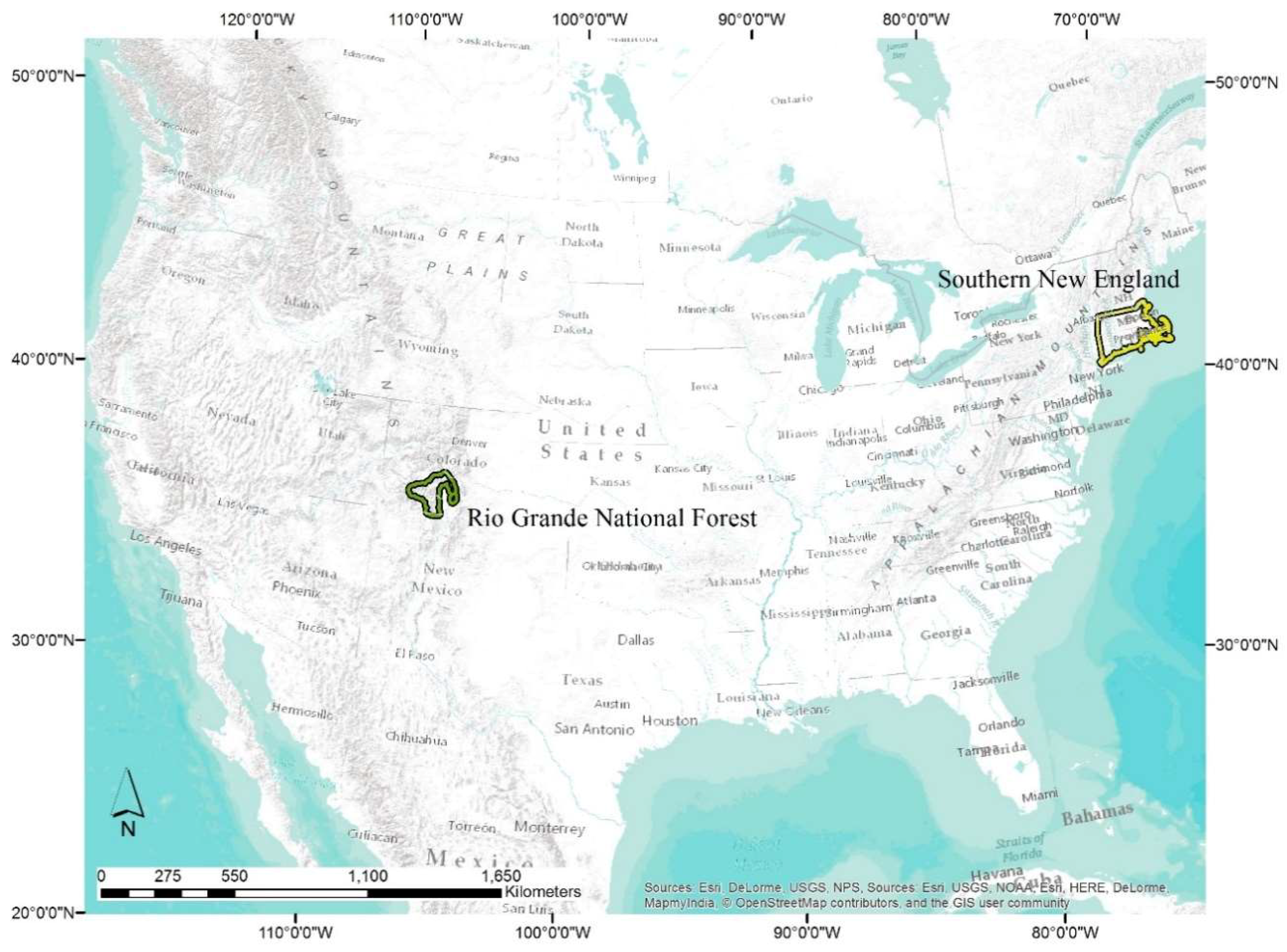
Article

An Evaluation of Forest Health Insect and Disease Survey Data and Satellite-Based Remote Sensing Forest Change Detection Methods: Case Studies in the United States

RedCastle Resources, Inc. Contractor to: USDA Forest Service Geospatial Technology and Applications Center (GTAC), Salt Lake City, UT 84119, USA
*
Author to whom correspondence should be addressed.
Remote Sens. 2018, 10(8), 1184; https://doi.org/10.3390/rs10081184
Submission received: 24 May 2018 / Revised: 10 July 2018 / Accepted: 18 July 2018 / Published: 27 July 2018
(This article belongs to the Special Issue Remote Sensing of Forest Cover Change)

Abstract

:
The Operational Remote Sensing (ORS) program leverages Landsat and MODIS data to detect forest disturbances across the conterminous United States (CONUS). The ORS program was initiated in 2014 as a collaboration between the US Department of Agriculture Forest Service Geospatial Technology and Applications Center (GTAC) and the Forest Health Assessment and Applied Sciences Team (FHAAST). The goal of the ORS program is to supplement the Insect and Disease Survey (IDS) and MODIS Real-Time Forest Disturbance (RTFD) programs with imagery-derived forest disturbance data that can be used to augment traditional IDS data. We developed three algorithms and produced ORS forest change products using both Landsat and MODIS data. These were assessed over Southern New England and the Rio Grande National Forest. Reference data were acquired using TimeSync to conduct an independent accuracy assessment of IDS, RTFD, and ORS products. Overall accuracy for all products ranged from 71.63% to 92.55% in the Southern New England study area and 63.48% to 79.13% in the Rio Grande National Forest study area. While the accuracies attained from the assessed products are somewhat low, these results are similar to comparable studies. Although many ORS products met or exceeded the overall accuracy of IDS and RTFD products, the differences were largely statistically insignificant at the 95% confidence interval. This demonstrates the current implementation of ORS is sufficient to provide data to augment IDS data.

Graphical Abstract

1. Introduction

The US Forest Service’s Forest Health Protection (FHP) program is tasked with protecting and improving the health of America’s rural, wildland, and urban forests. The Operational Remote Sensing (ORS) program was developed as a part of the Forest Health Assessment and Applied Sciences Team’s (FHAAST) Insect and Disease Survey (IDS) analysis and decision support tools. These tools assist FHP staff, state forestry agencies, and other forest managers to locate, monitor, and map forest health issues. FHAAST supports a number of technology development programs, such as ORS, to assist their partners, increase accuracy, and lower the cost of forest health protection.

1.1. Aerial Detection Survey

The ORS program was developed to address the data requirements of the IDS program. IDS is a collection of geospatial data depicting the extent of insect, disease, and other forest disturbance types. In the past, IDS data collection largely came from first-hand aerial observations and sketch mapping via the Aerial Detection Survey (ADS). Supplemental field surveys also contributed to the IDS database. Aerial sketch mapping is now conducted using either Digital Aerial Sketch Mapping (DASM) or Digital Mobile Sketch Mapping (DMSM) systems. These systems consist of tablet computers, GPS units, and specialized software that assist observers in an aircraft to map forest health issues [1]. While system improvements such as the more modern DMSM have increased the consistency and quality of the IDS data, they have not significantly reduced the number of hours spent flying. Time spent flying is an issue because conducting aerial surveys is both risky and costly. In 2010, an ADS pilot and two aerial surveyors were killed in an aviation accident [2]. While the need for reporting and analysis of ADS data remains, efforts are being made to integrate ground collection and satellite remote sensing to improve safety and quality of IDS data.

1.2. Remote Sensing Augmentation to IDS

The Real-Time Forest Disturbance (RTFD) program was designed to detect and track rapid onset forest change events (e.g., rapid defoliation and storm driven changes) as well as slow onset forest change events (e.g., insect induced mortality) across the CONUS on a weekly basis during the growing season [3]. The RTFD program serves as a near-real time alarm system to highlight forest disturbances in support of ADS mission planning by state and local forestry personnel. Because of the spatial coarseness of MODIS data and fixed parameters that are used to produce consistent RTFD products, the RTFD program does not necessarily yield spatially refined results that are sufficient to produce spatially explicit maps for the IDS database. In contrast, the goal of the ORS program is to augment the annually produced IDS data with a novel source of forest disturbance map products. To that end, satellite image data of higher spatial resolution relative to the MODIS-based RTFD program can be used, and change detection parameters can be fine-tuned for specific forest disturbance events.
ORS products do not contain disturbance agent information found in IDS data. The spatial resolution of the imagery used to generate data for ORS cannot compare to viewing forest disturbance phenomena from an airplane. Furthermore, no automated algorithm is commensurate to the experience accumulated over a career by an aerial detection surveyor observing the effects of pests and pathogens on forests. On the other hand, analysis performed using remote sensing imagery provides a consistent view of the landscape that is unobtainable by manually sketched maps by multiple interpreters. There are advantages and disadvantages associated with both sources of forest health spatial data. Therefore, the goal of the ORS program is to create forest change maps that provide a balance of spatial completeness, timeliness, and safety.
ORS data are produced as needed in response to a field request or an RTFD detection. ORS data may also be produced at the end of a growing season to supplement the annual IDS data stream. Thematic information contained in ORS maps includes non-tree, tree no change and tree change.

1.3. Change Detection Methods

The ORS program targets intra-seasonal change associated with insect defoliation and disease, as well as long-term decline in forest vigor associated with insects and pathogens. Prior to this work, many studies developed methods to meet different land cover change mapping/monitoring needs [4,5,6,7,8,9]. Early remote sensing change detection methods generally utilized two-date image pairs in various techniques to detect change [5]. These methods proved cost effective and computationally practical at the time.
After the Landsat archive became freely available to the general public in 2008, change detection methods that required annual or biennial time series image stacks of Landsat data became cost effective. Methods such as the Vegetation Change Tracker (VCT) [6] and Landsat-based detection of Trends in Disturbance and Recovery (LandTrendr) [7] were designed to detect and track changes that persist for more than a single growing season. Because VCT is designed to detect abrupt stand-clearing forest change events, it struggles to detect long-term and partial tree cover change events [9]. Neither of these methods is sensitive to intra-annual change.
As computational power increased, methods that utilize all available data throughout the year were developed. Breaks for Additive Seasonal and Trend (BFAST) [8] and Continuous Change Detection and Classification (CCDC) [10] use harmonic regression to account for seasonal variation, leaving the remaining variance to perform change analysis. The ability of these algorithms to detect change is largely a function of the frequent availability of cloud/cloud shadow-free data. The frequency must be sufficient to capture the typical seasonality of an area. The one-day revisit frequency of MODIS is likely to provide the necessary temporal density. The 16-day revisit frequency of Landsat is likely insufficient in areas frequently obscured by clouds.
While VCT, LandTrendr, BFAST, and CCDC excel at finding land cover changes across large areas that persist for more than a single observation, finding subtle changes that often only persist for a portion of a single growing season generally requires a more targeted approach. These methods are often referred to as “near-real time” [3,11]. Near-real time change detection methods generally compare analysis period observations to a stable baseline period. Because each observation in the analysis period is being compared to many observations in the baseline period, the algorithm can be more sensitive to the onset of subtle change. Some methods that utilize a baseline period and analysis period include the Z-score approach used in the USFS RTFD program [3], BFAST-Monitor [11], and Exponentially Weighted Moving Average Change Detection (EWMACD) [12]. The harmonic regression approach used in the latter two of these methods underpin the harmonic Z-score approach applied in this research.
While utilizing EWMACD and/or BFAST-Monitor to meet the needs of the ORS program would be appropriate, ORS required algorithms that were operative within Google Earth Engine (GEE) by spring 2015. At that time, neither of these algorithms was available within GEE, so we built on the ideas from the RTFD Program, EWMACD, and BFAST-Monitor that were practical to implement with GEE.
To compare ORS outputs and other existing FHP spatial products, we created ORS outputs in two geographically disparate study areas from three targeted change detection algorithms that were developed for the ORS project. These include the basic Z-score, harmonic Z-score, and linear trend analysis change detection methods. We then used reference data acquired using TimeSync [13], a time series visualization and data collection tool, to conduct an accuracy assessment to better understand how accurate ORS outputs are compared to RTFD and IDS data products [14,15].

2. Materials and Methods

2.1. Study Areas

We chose two study areas to evaluate the ability of the ORS program’s methods to map and monitor intra-seasonal and multi-year forest decline across different ecological settings (Table 1 and Figure 1).
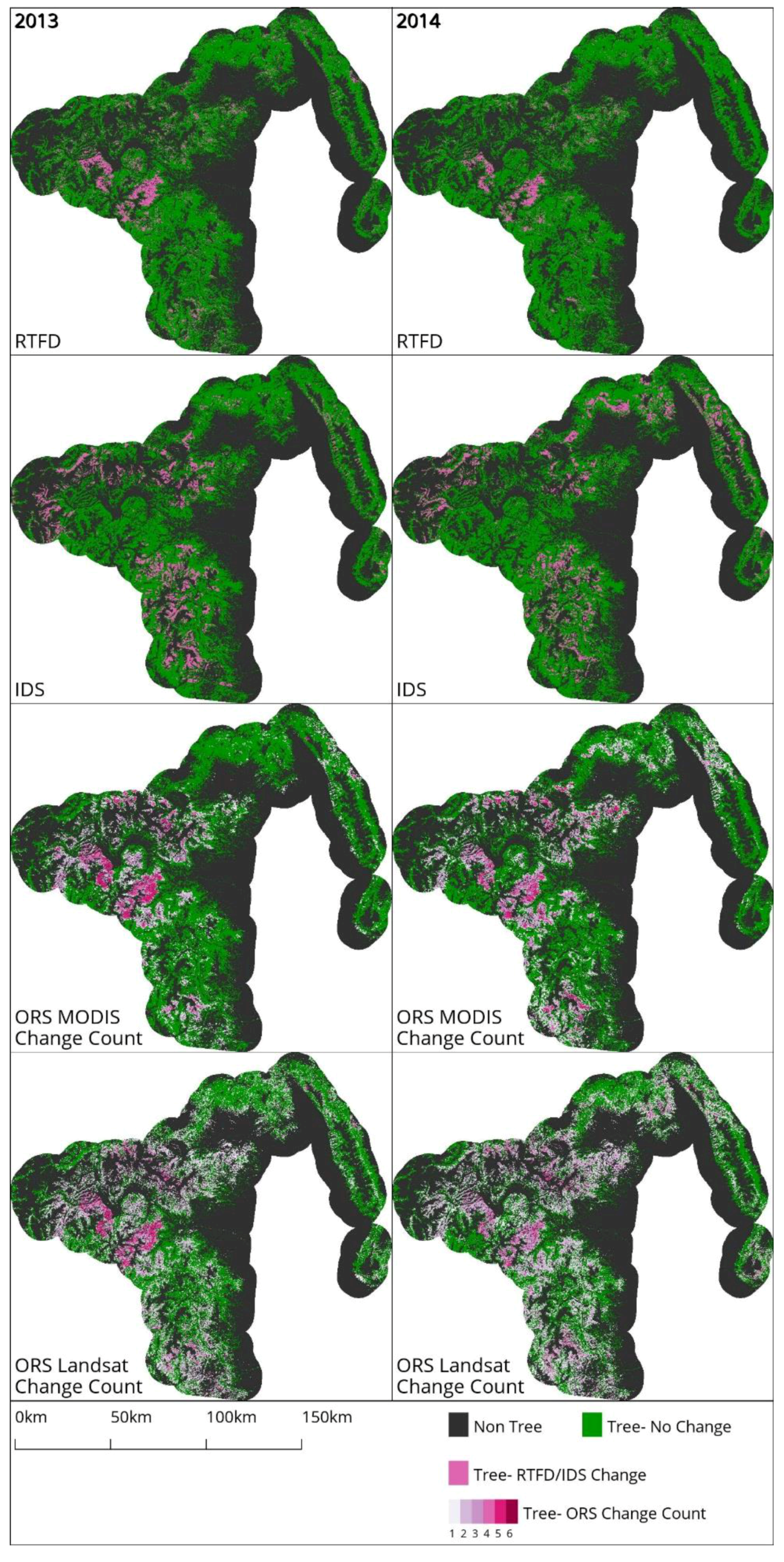
The Rio Grande National Forest study area captures a slow onset forest disturbance caused by mountain pine beetle (Dendroctonus ponderosae) and spruce bark beetle (Dendroctonus rufipennis). The Forest has been experiencing long-term gradual decline and mortality, with a total of 617,000 acres being infested by spruce beetles since 1996 [16]. Inclusion of this study area presents an opportunity to test the ability of the change algorithms to discern new areas of forest disturbance from areas affected in previous years.
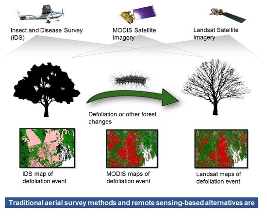
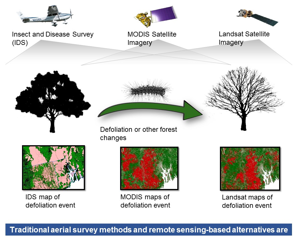
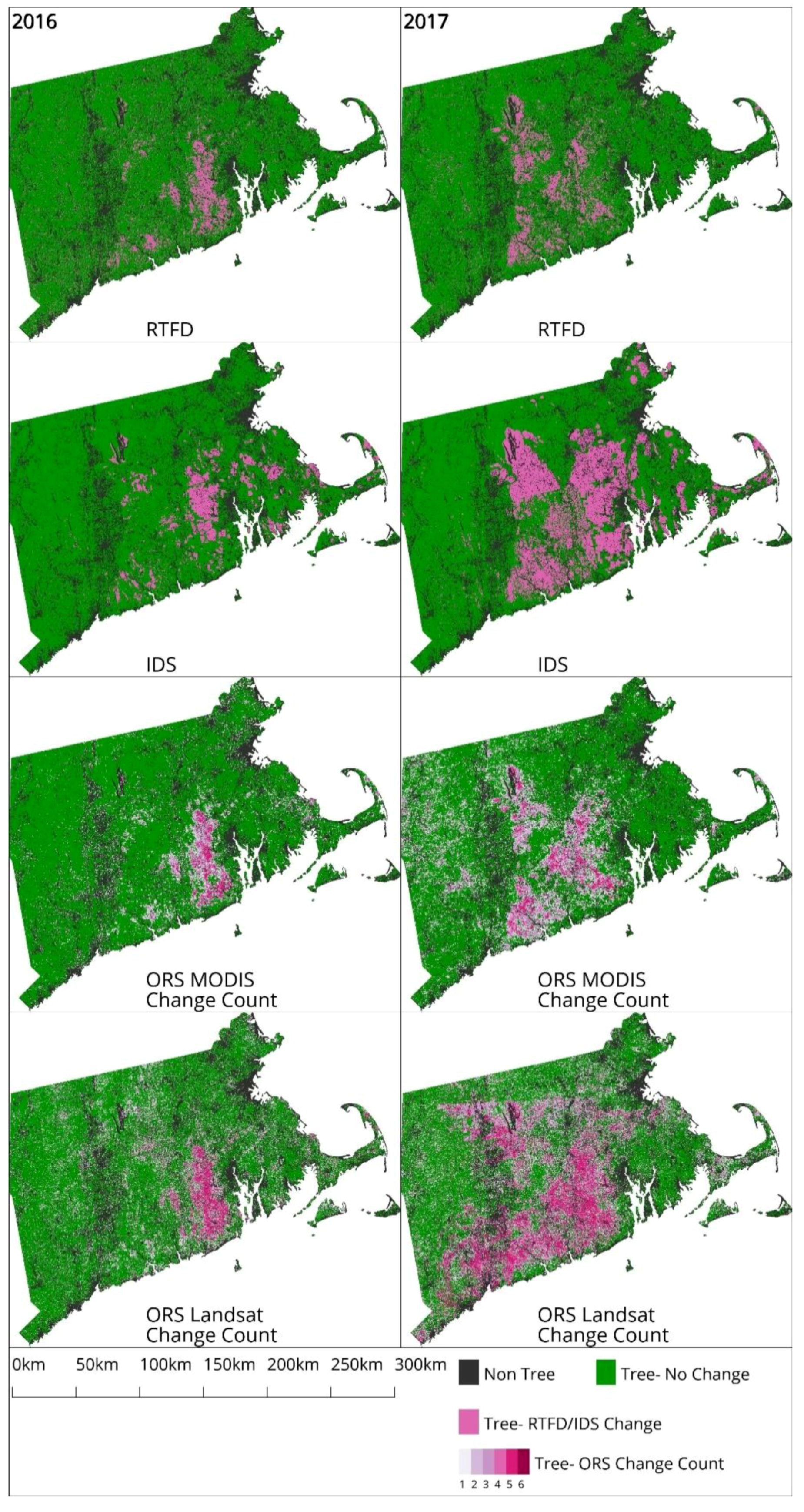
The Rhode Island, Massachusetts, and Connecticut (Southern New England) study area experienced extensive Gypsy Moth (Lymantria dispar dispar) defoliation events in 2016 and 2017. This region typifies many challenges associated with detecting ephemeral forest disturbances using remote sensing data. These challenges include the temporal variations in phenological conditions and persistent nature of cloud cover in the region.
Within each study area, we analyzed pixels that had a NLCD 2011 Tree Canopy Cover [17] value greater than 30 percent.

2.2. IDS-Data

We acquired IDS polygon data [1] for each study area. Surveyors collected these data using established aerial detection survey sketch mapping techniques by the USDA Forest Service. IDS data are used to estimate the spatial extents of forested areas disturbed by insects and diseases, as well as attribute the causal agents of these disturbances [1,18]. They are conducted using light aircraft, as well as ground surveys.
IDS data originated from separate aerial and ground surveys performed in Massachusetts, Connecticut, and Rhode Island during 7 June–25 August 2016 and 26 June–26 August 2017 for the Southern New England study area. Rio Grande National Forest study area IDS data were created from a wall-to-wall aerial survey of forested areas in Colorado conducted during 30 July–18 September 2013 and 24 June–3 September 2014.

2.3. RTFD-Data

RTFD persistence change data were incorporated into this study to compare with spatial data created using ORS methods. RTFD data are created for the entire CONUS every 8 days from 18 February to 24 November using 16-day MODIS composites. The RTFD approach employs a combination of two separate remote sensing change detection approaches to detect and track quick ephemeral changes in forest health as well as gradually occurring disturbances [3]. The first uses a statistical (z-score) change detection method for detecting quick intra-seasonal changes in forest conditions. The second approach uses linear regression to identify areas where slower, multiyear changes are occurring in forested areas. Disturbances were characterized using the RTFD z-score change detection method in Southern New England while the linear trend method was employed over the Rio Grande National Forest. In all study areas, the RTFD persistence output was used to spatially depict forest disturbances. The persistence RTFD output combines the results of the last three 16-day compositing period RTFD change outputs. This added processing step minimizes noise in individual compositing period outputs arising from persistent cloud cover and other MODIS ephemera. The persistence output collapses continuous RTFD z-score and linear trend outputs into three classes of disturbance magnitude by combining the disturbance frequency over the last three compositing periods with disturbance intensity based on departure from normal forest conditions [3]. The three disturbance magnitude classes were collapsed into binary disturbance maps for use in this study.
RTFD data used in this study were produced during 10 June–27 July 2016 and 26 June–12 August 2017 for the Southern New England study area and during 28 July–28 August for both analysis years for the Rio Grande National Forest study area.

2.4. ORS-Data

ORS methods were built using satellite image data that had been collected for at least 5 years and would likely be regularly available into the future. This includes imagery from Landsat Thematic Mapper (TM, 1984–2011), Enhanced Thematic Mapper (ETM+, 1999–Present), and Operational Land Imager (OLI, 2013-Present). Each Landsat sensor has a revisit frequency of 16 days. Since Landsat 5 and 7 overlapped during 1999–2011 and Landsat 7 and 8 overlapped during 2013–present, these periods have a revisit frequency of about 8 days. All Landsat-based analyses were conducted at 30 m spatial resolution.
ORS methods were also applied to MODerate-resolution Imaging Spectroradiometer (MODIS) imagery collected from the Terra (1999–present) and Aqua (2002–present) satellites, which is available multiple times a day for most locations on Earth. MODIS imagery has a spectral resolution similar to Landsat, but coarser spatial resolution than Landsat. All MODIS-based analyses were conducted at 250 m spatial resolution.
This project utilized Landsat Ecosystem Disturbance Adaptive Processing System (LEDAPS) surface reflectance values from Landsat 5 and 7 [19], Landsat 8 Surface Reflectance Code (LaSRC) values for Landsat 8 [20], and MODIS Terra and Aqua 8-day surface reflectance composites. All data were accessed through Google Earth Engine, which acquires MODIS data from the NASA Land Processes Distributed Active Archive Center (LP DAAC), USGS/Earth Resources Observation and Science (EROS) Center, Sioux Falls, South Dakota, and Landsat data from EROS Center, Sioux Falls, South Dakota. LP DAAC MODIS collections used are found in Table 2.

2.5. Data Preparation

All data preparation and analysis were performed with Google Earth Engine (GEE). GEE provides access to most freely available earth observation data and provides an application programming interface (API) to analyze and visualize these data [21].
All Landsat images first underwent pixel-wise cloud and cloud shadow masking using the Google cloudScore algorithm for cloud masking and Temporal Dark Outlier Mask (TDOM) for cloud shadows. Since neither of these methods is currently documented in the peer-reviewed literature, they are briefly described below, and are fully described and evaluated in a forthcoming paper [22]. MODIS 8-day composites are intended to be cloud-free, so no pre-processing was conducted.
The Google cloudScore algorithm exploits the spectral and thermal properties of clouds to identify and remove these artifacts from image data. To simplify the process, the cloudScore function uses a min/max normalization function to rescale expected reflectance or temperature values between 0 and 1 (Equation (1)). The algorithm applies the normalization function to five cloud spectral properties. The final cloudScore is the minimum of these normalized values (Equation (2)). The algorithm finds pixels that are bright and cold, but do not share the spectral properties of snow. Specifically, it defines the cloud score as:
n o r m a l i z e ( b ,   x m i n , x m a x ) = b x m i n x m a x x m i n
c l o u d S c o r e l a n d s a t = min { 1.0 ,   n o r m a l i z e ( b l u e , 0.1 , 0.3 ) ,   n o r m a l i z e ( b l u e + g r e e n +   r e d , 0.2 , 0.8 ) ,   n o r m a l i z e ( n i r + s w i r 1 + s w i r 2 , 0.3 , 0.8 ) , n o r m a l i z e ( t e m p , 300 , 290 ) ,   n o r m a l i z e ( g r e e n     s w i r 1 g r e e n   +   s w i r 2 , 0.8 , 0.6 ) }
Any pixel with a cloudScore value greater than 0.2 was identified as being a cloud. This value was qualitatively evaluated through extensive use throughout the CONUS to provide the best balance of detecting clouds, while not committing cold, bright surfaces. Any values inside the resulting mask were removed from subsequent steps of the analysis.
After clouds were masked, cloud shadows were identified and masked. Since the Landsat archive is extensive across time, cloud shadows generally appear as anomalously dark pixels. GEE provides access to the entire archive of Landsat, enabling methods that require querying extensive time series of data. The Temporal Dark Outlier Mask (TDOM) method was used to identify pixels that are dark in relative and absolute terms. Generally, pixels will not always be obscured by a cloud shadow, making this method effective. Specifically:
z ( M b ) = M b M ¯ b σ b
d a r k n e s s = M s w i r 1 + M n i r
c l o u d S h a d o w = A l l { z ( M s w i r 1 ) < t Z S ,   z ( M n i r ) < t Z S ,   d a r k n e s s < t I R }
where M ¯ b and σ b are the mean and standard deviation, respectively, of a given band b across the time series, M is the multispectral Landsat image, t Z S is the threshold for the shadow z-score (−1 for this study), and t I R is the threshold for the d a r k n e s s (0.35 for this study).
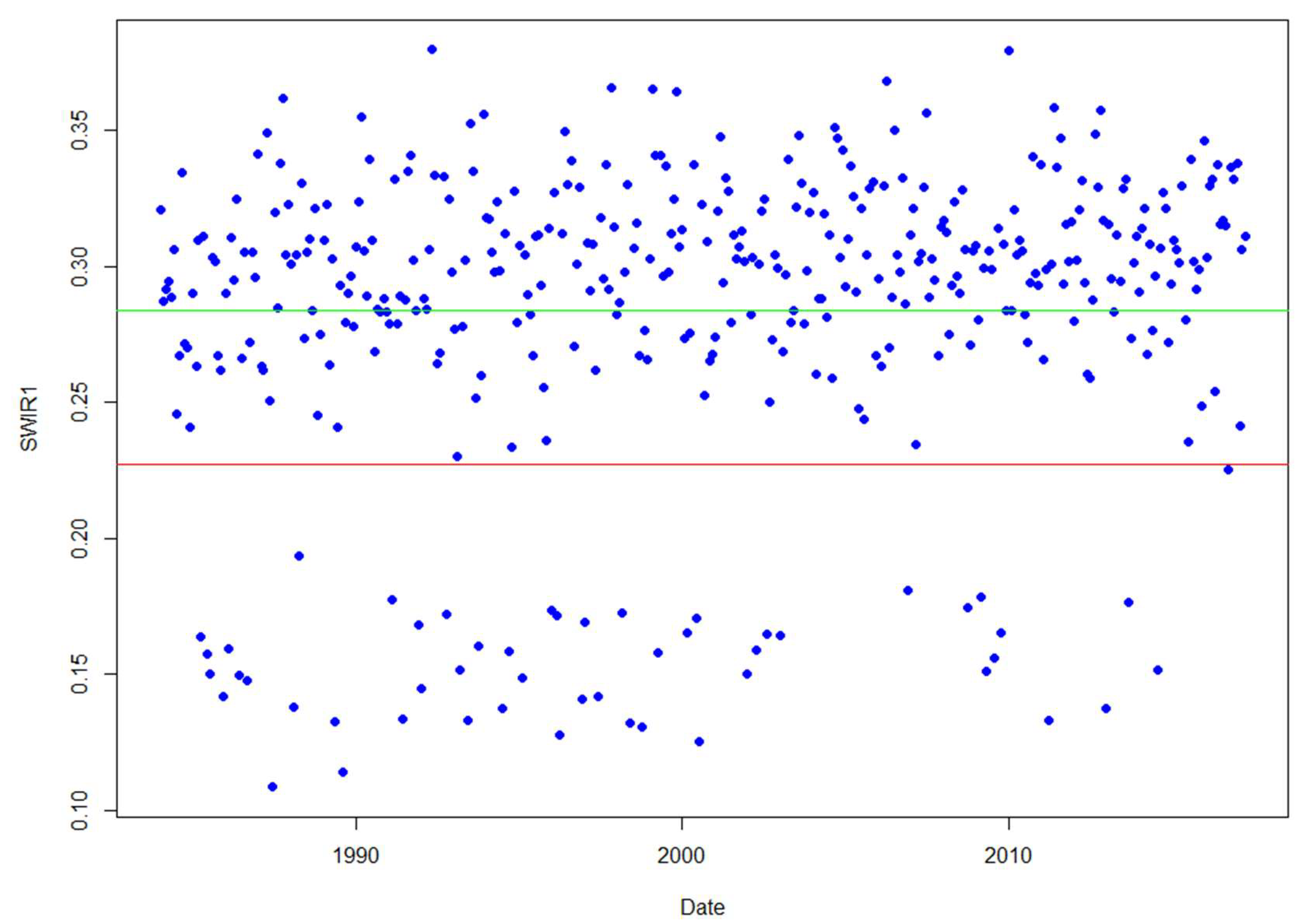
The TDOM method first computes the mean ( M ¯ b ) and standard deviation (σb) of the near-infrared (NIR) and shortwave-infrared (SWIR1) bands across a collection of images. For each image, the algorithm then computes the z-score of the NIR and SWIR1 bands (z(Mb)) (Equation (5)) (Figure 2). Each image also has a darkness metric computed as the sum of the NIR and SWIR1 bands ( d a r k n e s s ). Cloud shadows are then identified if a pixel has a z-score of less than −1 for both the NIR and SWIR1 bands and a darkness value less than 0.35 (Equation (8)). These thresholds were chosen after extensive qualitative evaluation of TDOM outputs from across the CONUS.
This study used the normalized difference vegetation index (NDVI) (Equation (6)) [23] and the normalized burn ratio (NBR) (Equation (7)) [24] as indices of forest greenness to detect forest changes.
N D V I = N I R r e d N I R + r e d ,
N B R = N I R S W I R 2 N I R + S W I R 2 ,
where NIR is the near infrared band of a multispectral image, red is the red band of a multispectral image, and SWIR2 is the second shortwave infrared band of a multispectral image. Many additional common indices are available for use when running ORS algorithms, but were omitted from this study. These two indices are used since the bands necessary to create them are available for both MODIS and Landsat, they are very similar to the indices used in the RTFD program, and they have proven effective throughout the remote sensing change detection literature [6,7,11,23,24].

2.6. Change Detection Algorithms

Three algorithms were developed and tested in GEE using MODIS and Landsat data. Employing GEE for this study enabled us to efficiently test various change detection approaches using Landsat and MODIS image data archives, without downloading and storing the data locally.
ORS mapping needs fell into two categories: ephemeral change related to defoliation events and long-term change related to tree mortality from insects and disease. The three algorithms used in this study were selected to address the needs posed by these forest change types. We refer to these algorithms as: basic z-score (Figure 3), harmonic z-score (Figure 4), and linear trend (Figure 5).
The basic z-score method builds on ideas from RTFD, serving as a natural starting point for ORS mapping methods. The harmonic z-score method combines ideas from harmonic regression-based methods, such as EWMACD [12] and BFAST Monitor [11], with those from the basic z-score method to leverage data from throughout the growing season. The linear trend method is built on ideas from Image Trends from Regression Analysis (ITRA) [25] and the RTFD trend method [3]. It uses linear regression to fit a line across a series of years.
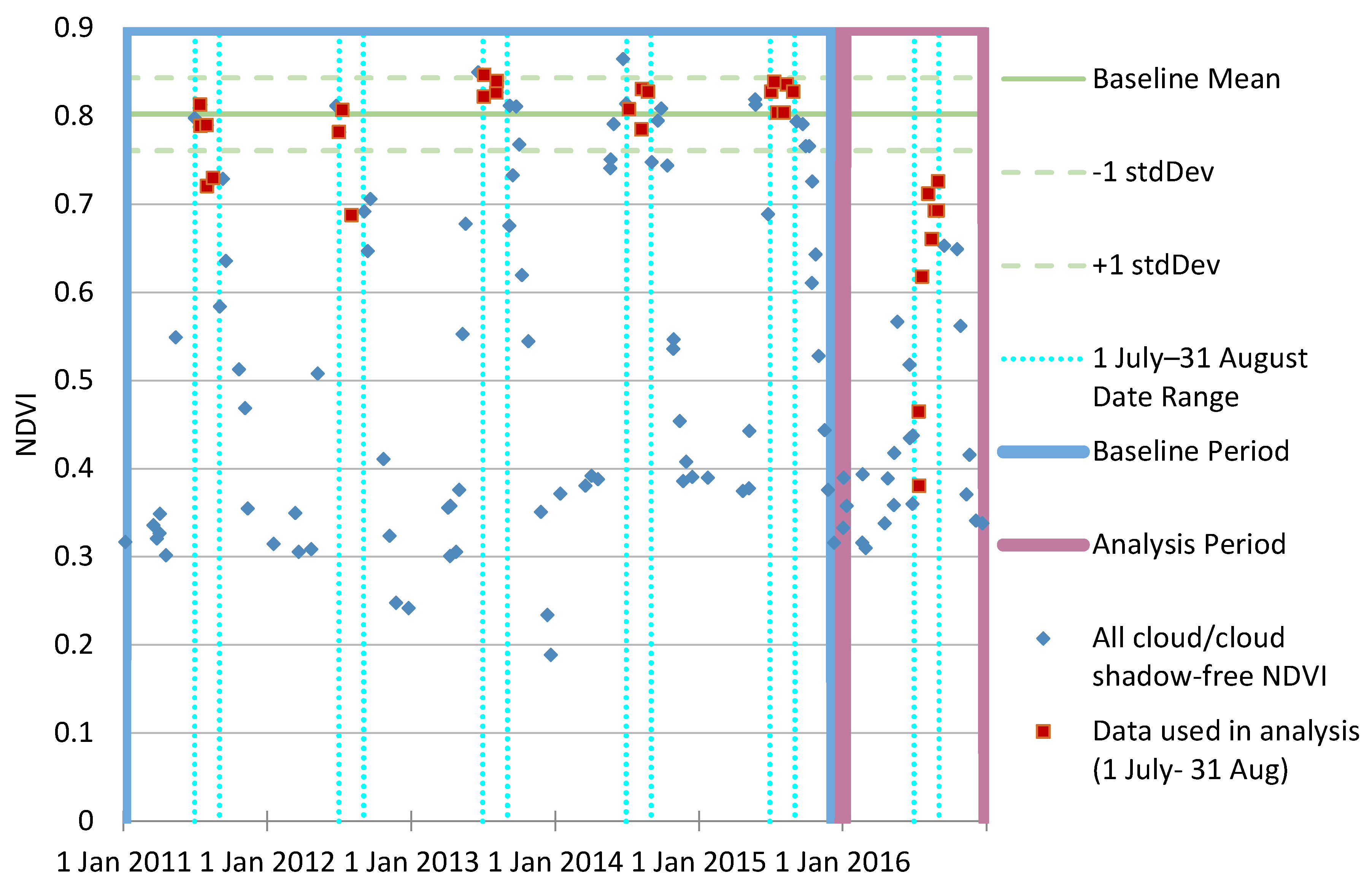
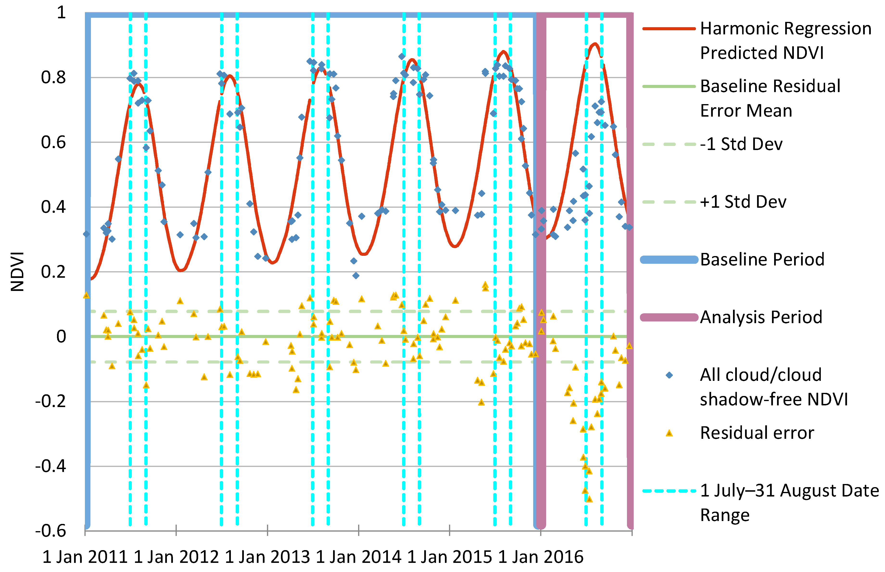
Both the basic z-score and harmonic z-score method work by identifying pixels that differ from a baseline period. The primary difference is what data are used to compute the z-score. Both methods start by acquiring imagery for a baseline period (generally 3–5 years) and analysis years. The basic z-score method uses the mean and standard deviation of the baseline period within a targeted date range for a specified band or index, while the harmonic z-score method follows the EWMACD and BFAST Monitor methods by first fitting a harmonic regression model to all available cloud/cloud shadow-free Landsat or MODIS data.
The harmonic regression model is intended to mitigate the impact of seasonality on the spectral response, leaving remaining variation to be related to change unrelated to phenology. The harmonic is defined as:
y b = a 0 b + a 1 b t + a 2 b cos ( 2 π t ) + a 3 b sin ( 2 π t )
where b is the band or index of the image, a n b are the coefficients being fit by the model, and t is the sum of the date expressed as a year and the proportion of a year.
The harmonic regression model is fitted on a pixel-wise basis to the baseline data and then applied to both the baseline and the analysis data. Next, the residual error is computed for both the baseline and analysis data. Up to this point, the harmonic z-score method, EWMACD, and BFAST Monitor methods are largely the same. The primary difference with these three methods is how change is classified. While EWMACD and BFAST Monitor use exponentially weighted moving average (EWMA) charting and moving sum (MOSUM) of the residuals, respectively [11,12], the harmonic z-score method uses the mean and standard deviation of the targeted date period baseline residuals to compute the z-score of the targeted analysis period residuals. The date range and specific years used to define the baseline can be tailored to optimize the discernment of specific disturbances within the analysis years.
Since an analysis period may have more than a single observation, a method for summarizing these values is specified for both the basic and harmonic z-score methods to constrain the final z-score value. For this study, the mean of values was used. Change is then identified by thresholding the summary z-score value. For this project, summarized z-score values less than −0.8 were identified as change. This threshold was chosen based on analyst expertise obtained from iterative qualitative comparison of z-score results with post-disturbance image data.
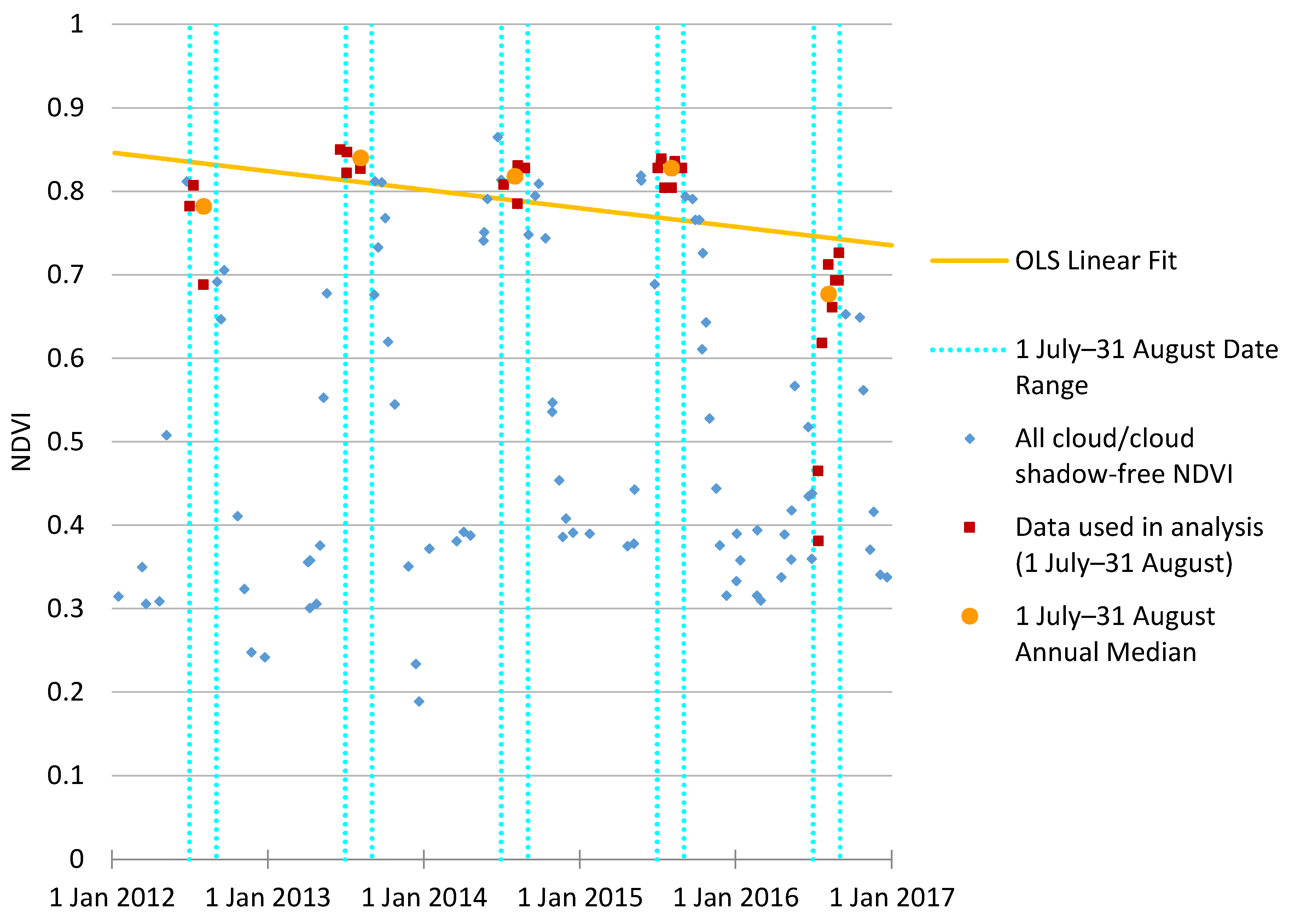
The linear trend method makes use of the median of the cloud and cloud shadow-free observations available within a specified target date period. This is done for a specified number of years prior to the analysis year, referred to as an epoch. For an epoch, an ordinary least square linear regression model is fit on a pixel-wise basis as follows:
y b = a 0 b + a 1 b t b
where b is the band or index of image, a0 is the intercept, a1 is the slope, t is the date, and y is the predicted value.
Change is identified where the slope (a1) is less than a specified threshold. The threshold used for this study was −0.03. This was chosen based on analyst expertise similar to the identification of the threshold used for the z-score methods. This method differs from ITRA [25] since it does not use a t-test to classify change.
ORS methods differ from existing RTFD methods in several key areas. Firstly, RTFD products are created in a near-real time environment that GEE cannot currently provide. The composites that are used are therefore slightly different than those used in ORS. Secondly, all baseline statistics are computed on a pixel-wise basis for ORS methods, while they are computed on a zone-wise basis for RTFD methods—where the zones are defined by the combination of USGS mapping zone, forest type, and MODIS look angle strata [3]. The most pronounced difference, however, is that all model input parameters for RTFD are fixed, while ORS parameters can be tailored to a specific forest disturbance event by an expert user.
We tested all three methods in both study areas. Analysts chose targeted date ranges based on expert knowledge of when each event was most visible. For the Southern New England study area, ORS analyses were conducted between 25 May and 9 July for both 2016 and 2017. Baseline years spanned 2011–2015 for harmonic z-score and regular z-score methods while a three-year epoch length was used for the linear trend method. For the Rio Grande National Forest study area, ORS analyses were conducted from 9 July to 15 October for 2013 and 2014. Baseline years spanned 2007–2011 for harmonic z-score and regular z-score methods while a five-year epoch length was used for the linear trend method.

2.7. Accuracy Assessment Methods

We performed an independent accuracy assessment to understand how well ORS products performed relative to existing FHP disturbance mapping programs. We followed best practices for sample design, response design, and analysis as outlined by Olofsson et al. (2014) [26] and Pontius and Millones (2011) [27]. We drew a simple random sample across all 30 m × 30 m pixels that were within each study area’s tree mask. Since all change detection for this study was performed retrospectively, timely field reference data could not be collected. Instead, we collected independent reference data using TimeSync [13]. TimeSync is a tool that enables a consistent manual inspection of the Landsat time series along with high resolution imagery found within Google Earth. Single Landsat pixel-size (30 m × 30 m) plots were analyzed throughout the baseline and analysis periods. The response design was created for the US Forest Service Landscape Change Monitoring System (LCMS) [28] and USGS Landscape Change Monitoring Assessment and Projection (LCMAP) [29] projects to provide consistent depictions of land cover, land use, and change process. Rigorous analyst training and calibration was used to overcome the subjective nature of analyzing data in this manner. We analyzed 230 plots across the Rio Grande National Forest and 416 plots across the Southern New England study area. We then cross-walked all responses for each year to change and no change. For consistency, all ORS, IDS, and RTFD outputs had the same 30 m spatial resolution tree mask used for drawing the reference sample applied to them. All MODIS-based ORS and RTFD outputs were resampled from 250 m to 30 m spatial resolution using nearest neighbor resampling. The reference data was then compared to each of the ORS outputs along with the IDS and RTFD products for each analysis year. Accuracy metrics follow suggestions by Pontius and Millones (2011) [27]. They include those related to allocation disagreement (overall accuracy, and class-wise omission and commission error rates) and quantity disagreement (reference and predicted prevalence). The 5th and 95th percentile confidence interval was calculated using the overall accuracy of 500 bootstrap random samples for each assessed output. While these methods provide a depiction of the accuracy of the assessed change detection methods within the tree mask, it completely omits any areas outside of this mask from all analyses.

3. Results

The reference dataset produced using TimeSync for each analysis year was compared to each of the 12 ORS outputs, as well as the RTFD and IDS outputs. The 12 ORS outputs reflect the combination of basic z-score, harmonic z-score, and trend analysis methods, calculated using either NDVI or NBR greenness indices, and derived from either Landsat or MODIS data.

3.1. Southern New England

The overall accuracy of all outputs ranges from 84.86% to 92.55% in 2016 and 71.63% to 87.02% in 2017 (Table 3 and Table 4). The overall accuracies are largely insignificantly different from one another with respect to the 5th and 95th percentile confidence intervals. The proportion of plots the reference data indicates has changed is sometimes similar to the map outputs while others are different in relative and absolute terms. This result can be found in the tree change prevalence columns in Table 3 and Table 4. The highest overall accuracy and lowest commission, omission, and prevalence error rates are highlighted in each table. The ORS trend algorithm has the highest overall accuracy and lowest change prevalence error for both 2016 and 2017. Omission and commission error rates are quite varied and inconsistent across different combinations of algorithm, platform, and index. Many ORS outputs perform as well or better than IDS and RTFD outputs for both years.
The patterns of spatial agreement are evident in Figure 6, where a heat map of the number of ORS outputs that found a pixel as change are displayed with the corresponding IDS and RTFD (z-score) maps. Overall spatial patterns are similar between each product. There is a notable similarity between the RTFD maps and MODIS-based ORS maps. This reflects the similarities between the source data and methods used to derive these maps.

3.2. Rio Grande National Forest

The southwestern United States, including the Rio Grande National Forest study area, has been impacted for the last 20 years by prolonged drought conditions, contributing to slow-onset insect infestations including mountain pine beetle and spruce bark beetle [24,28]. This study focused on the change that occurred in 2013 and 2014.
The overall accuracy of products obtained for the Rio Grande study area are lower than the Southern New England study area—ranging from 63.48% to 79.13% in 2013 and 66.09% to 76.09% in 2014 (Table 5 and Table 6). Similar to the results from Southern New England, the overall accuracies are largely insignificantly different. The tree change prevalence error is a bit higher for most outputs in the Rio Grande study area: it is underestimated by as much as 26.09% (88.23% quantity error) and overestimated by as much as 22.61%. In general, the linear trend ORS method performed the best for both the 2013 and 2014 outputs. This is not surprising due to the gradual nature of tree decline and mortality caused by the bark beetle activity that has been occurring in this study area.
The heat map in Figure 7 shows different patterns of spatial agreement and disagreement than we observed in the Southern New England study area. The first notable difference is that both RTFD and ORS methods continue to capture areas that changed in both 2013 and 2014, while IDS maps only show new areas of change in 2014. This difference is inherent in the underlying methods, as IDS will often not remap previously existing long-term change. The second notable difference is that the area of new tree change in 2014 in the northeast portion of the study area was largely missed by RTFD, but was captured by both IDS and many ORS methods.

4. Discussion

This study improves our understanding of how well ORS algorithms perform compared to existing FHP mapping programs and provides an idea of how well these algorithms perform relative to other similar algorithms.
All methods have similar overall accuracies and highly variable omission and commission error rates. Placing this study in the context of recent forest change detection research, some similarity in results can be found. Cohen et al. (2017) [15] provided an accuracy assessment of several change algorithms, while Brooks et al. (2017) [30] examined EWMACD and a newer adaptation of EWMACD called dynamic EWMACD (Edyn). Both studies use TimeSync to gather reference data. Cohen et al. (2017) found omission and commission error rates for EWMACD (similar to ORS harmonic z-score method) and ITRA (similar to ORS trend method) are greater than 70%. This is a higher error rate than most results in this study. Brooks et al. (2017) find EWMACD has a 65.2% omission error rate and 39.9% commission error rate [30].
While the omission and commission error rates seem to generally be high when using reference data from TimeSync, Cohen et al. (2017) [15] assert that the level of disagreement between the TimeSync-based reference data and outputs from automated algorithms can occur for many reasons. They acknowledge that change detection methods are now trying to detect more subtle changes and therefore TimeSync-based response designs (such as the one used in this study) now include lower magnitude disturbances. TimeSync’s strength is that it relies on utilizing more than just Landsat data, and leverages a human interpreter’s ability to discern subtle changes. They recognize this leads to higher commission/omission error rates than earlier change detection accuracy assessments. This is not to say TimeSync reference data over-estimate change, but rather highlights that individual automated change detection algorithms can only attain a finite level of sensitivity to change.
While the results obtained in this study are comparable to those obtained in other change detection studies, we must also evaluate the accuracy of these map outputs relative to each other. Various accuracy measures demonstrate that ORS outputs often perform comparably or better than IDS or RTFD products. Since there are several ORS outputs that were out-performed by IDS and/or RTFD outputs, the importance of choosing the best ORS method and parameters for a given mapping task is evident. Future work to quantitatively optimize the parameters used in ORS algorithms will be conducted to address this need.
In the meantime, ORS outputs will continue to be qualitatively calibrated. This may call into question the utility of the ORS program in its current form. While the importance of quantitative calibration cannot be understated, the ORS program has been qualitatively calibrating these algorithms for three growing seasons. Our experience indicates that the harmonic z-score algorithm is very difficult to qualitatively calibrate and produces highly inconsistent results. Both the trend and regular z-score methods have consistently produced satisfactory results. These findings largely agree with the results of this study.
Despite having coarser spatial resolution, MODIS-based outputs often out-performed equivalent Landsat-based outputs. This likely is related to the differences between their temporal resolution. The limited availability of cloud/cloud shadow-free Landsat images hinders its utility to consistently detect ephemeral forest disturbances that must be captured within narrow time windows. The frequent observations from MODIS permit a much greater opportunity to detect such disturbances.
While largely unapparent in the accuracy assessment results, IDS data exhibit unique characteristics not found in RTFD or ORS outputs. Firstly, whereas the ORS and RTFD change data are derived from space-borne satellite imagery from Landsat and MODIS platforms, the IDS data are derived from observations made by state and local forestry personnel from ground surveys or an aerial vehicle (e.g., fixed-wing aircraft or helicopter). Secondly, there is a range of methods used to compile IDS data on a state-by-state basis. The inconsistent methods employed to produce IDS data on a local level are evident in the Southern New England study area, where large polygons are favored in Massachusetts, smaller polygons are more common in Connecticut, and grid cells are the primary spatial unit in Rhode Island (Figure 8). In contrast, the results obtained from forest change detection algorithms using satellite imagery do not vary from place to place, but rather maintain an objective quality over space and time. This is likely why varying levels of agreement were seen between IDS data and the ORS and RTFD spatial results within the two study areas.
This study did not use Sentinel-2 Multispectral Instrument data, as their availability remains sparse over North America [31]. These data are also freely available, regularly collected, and have similar spatial resolution and spectral response functions to those of Landsat [32]. The spatial and spectral similarity of Sentinel-2 and Landsat suggests that these image data could be combined for hybrid analyses. Such hybrid approaches would increase the revisit frequency from every eight days with Landsat 7 and 8 to a range of everyday to every five days. Future work that incorporates these data to create ORS products will likely improve the quality of non-MODIS-based outputs by providing more temporally dense data to detect and track ephemeral forest disturbances.

5. Conclusions

This study tested three algorithms developed to map forest change for the USDA Forest Service’s FHP. Utilizing GEE as a platform to create these spatial data products was efficient and effective. ORS, IDS, and RTFD forest change products exhibited similar overall accuracy, and omission and commission error rates to other studies that used TimeSync to assess forest change products. The ORS spatial data often had similar or higher accuracy than existing FHP mapping program outputs. A unique strength of ORS spatial data lies in the adaptive nature of the algorithms employed. In contrast to the standardized method employed to create data for the RTFD program, the ability to adjust model parameters based on the characteristics of specific disturbance events permits the tuning of ORS spatial products. Additionally, the flexibility to use either Landsat scale or MODIS satellite image data in ORS algorithms permits the collection of timely synoptic observations regardless of the ephemeral nature of intra-seasonal forest disturbances.
While this study highlights that assessed FHP products have high error rates, real-world use has demonstrated their utility for spatially characterizing ephemeral and long term forest disturbances. ORS data have been used to augment the 2017 annual IDS database in the Southern New England study area for disturbances that occurred after the annual ADS had concluded [33]. In future years, data from ORS models will also be used to respond to local disturbance reports from counties, states, and forest units.

Author Contributions

Conceptualization, I.W.H., R.A.C., and M.V.F.; Methodology, I.W.H., R.A.C., and M.V.F.; Software, I.W.H.; Validation, I.W.H. and R.A.C.; Formal Analysis, I.W.H.; Investigation, I.W.H. and R.A.C.; Resources, M.V.F.; Data Curation, I.W.H.; Writing-Original Draft Preparation, I.W.H., R.A.C., and M.V.F.; Writing-Review & Editing, I.W.H., R.A.C., and M.V.F.; Visualization, I.W.H.; Project Administration, I.W.H. and M.V.F.; Funding Acquisition, M.V.F.

Funding

This research was funded by the US Forest Service, Geospatial Technology and Applications Center (GTAC) in support of applications being developed for the Forest Health Assessment and Applied Sciences Team (FHAAST).

Acknowledgments

The authors would like to acknowledge the assistance of members of the Google Earth Engine team—specifically Noel Gorelick and Matthew Hancher—in the design, execution, and analysis using Earth Engine. Lastly, we wish to acknowledge the many useful contributions of other RedCastle Resources and Forest Service technical personnel. Three anonymous reviewers also offered helpful critique and valuable recommendations for this paper.

Conflicts of Interest

The authors declare no conflict of interest.

References

  1. United States Department of Agriculture. Detection Surveys Overview. Available online: https://www.fs.fed.us/foresthealth/technology/detection_surveys.shtml (accessed on 19 September 2017).
  2. United States Department of Agriculture. FY10 Mishap Review. Available online: https://www.fs.fed.us/fire/av_safety/assurance/mishaps/FY10_Mishap_Review.pdf (accessed on 21 September 2017).
  3. Chastain, R.A.; Fisk, H.; Ellenwood, J.R.; Sapio, F.J.; Ruefenacht, B.; Finco, M.V.; Thomas, V. Near-real time delivery of MODIS-based information on forest disturbances. In Time Sensitive Remote Sensing; Lippitt, C.D., Stow, D.A., Coulter, L.L., Eds.; Springer: New York, NY, USA, 2015; pp. 147–164. ISBN 978-1-4939-2601-5. [Google Scholar]
  4. Coppin, P.R.; Bauer, M.E. Change detection in forest ecosystems with remote sensing digital imagery. Remote Sens. Rev. 1996, 13, 207–234. [Google Scholar] [CrossRef]
  5. Lu, D.; Mausel, P.; Brondizio, E.; Moran, E. Change detection techniques. Int. J. Remote Sens. 2004, 25, 2365–2407. [Google Scholar] [CrossRef]
  6. Huang, C.; Goward, S.; Masek, J.; Thomas, N.; Zhu, Z.; Vogelmann, J. An automated approach for reconstructing recent forest disturbance history using dense Landsat time series stacks. Remote Sens. Environ. 2010, 114, 183–198. [Google Scholar] [CrossRef]
  7. Kennedy, R.; Yang, Z.; Cohen, W. Detecting trends in forest disturbance and recovery using Landsat time series: 1. LandTrendr—Temporal segmentation algorithms. Remote Sens. Environ. 2010, 114, 2897–2910. [Google Scholar] [CrossRef]
  8. Verbesselt, J.; Hyndman, R.; Newnham, G.; Culvenor, D. Detecting trend and seasonal changes in satellite image time series. Remote Sens. Environ. 2010, 114, 106–115. [Google Scholar] [CrossRef]
  9. Stueve, K.M.; Housman, I.W.; Zimmerman, P.L.; Nelson, M.D.; Webb, J.B.; Perry, C.H.; Chastain, R.A.; Gormanson, D.D.; Huang, C.; Healey, S.P.; et al. Snow-covered Landsat time series stacks improve automated disturbance mapping accuracy in forested landscapes. Remote Sens. Environ. 2011, 115, 3203–3219. [Google Scholar] [CrossRef]
  10. Zhu, Z.; Woodcock, C. Continuous change detection and classification of land cover using all available Landsat data. Remote Sens. Environ. 2014, 144, 152–171. [Google Scholar] [CrossRef]
  11. Verbesselt, J.; Zeileis, A.; Herold, M. Near real-time disturbance detection using satellite image time series. Remote Sens. Environ. 2012, 123, 98–108. [Google Scholar] [CrossRef]
  12. Brooks, E.B.; Wynne, R.H.; Thomas, V.A.; Blinn, C.E.; Coulston, J.W. On-the-Fly massively multitemporal change detection using statistical quality control charts and Landsat data. IEEE Trans. Geosci. Remote Sens. 2014, 52, 3316–3332. [Google Scholar] [CrossRef]
  13. Cohen, W.B.; Yang, Z.; Kennedy, R. Detecting trends in forest disturbance and recovery using yearly Landsat time series: 2. TimeSync—Tools for calibration and validation. Remote Sens. Environ. 2010, 114, 2911–2924. [Google Scholar] [CrossRef]
  14. Griffiths, P.; Kuemmerle, T.; Kennedy, R.E.; Abrudan, I.V.; Knorn, J.; Hostert, P. Using annual time-series of Landsat images to assess the effects of forest restitution in post-socialist Romania. Remote Sens. Environ. 2012, 118, 199–214. [Google Scholar] [CrossRef]
  15. Cohen, W.B.; Healey, S.P.; Yang, Z.; Stehman, S.V.; Brewer, C.K.; Brooks, E.B.; Gorelick, N.; Huang, C.; Hughes, M.J.; Kennedy, R.E.; et al. How similar are forest disturbance maps derived from different Landsat time series algorithms? Forests 2017, 8, 98. [Google Scholar] [CrossRef]
  16. United States Forest Service. Available online: https://www.fs.usda.gov/detailfull/riogrande/home/?cid=stelprdb5409285&width=full (accessed on 15 May 2018).
  17. Ruefenacht, B.; Benton, R.; Johnson, V.; Biswas, T.; Baker, C.; Finco, M.; Megown, K.; Coulston, J.; Winterberger, K.; Riley, M. Forest service contributions to the national land cover database (NLCD): Tree Canopy Cover Production. In Pushing Boundaries: New Directions in Inventory Techniques and Applications: Forest Inventory and Analysis (FIA) Symposium 2015, Portland, OR, USA, 8–10 December 2015; Stanton, S.M., Christensen, G.A., Eds.; U.S. Department of Agriculture, Forest Service, Pacific Northwest Research Station: Portland, OR, USA, 2015; pp. 241–243. [Google Scholar]
  18. Johnson, E.W.; Wittwer, D. Aerial Detection Surveys in the United States. In Monitoring Science and Technology Symposium: Unifying Knowledge for Sustainability in the Western Hemisphere Proceedings RMRS-P-42CD; Aguirre-Bravo, C., Pellicane, P.J., Burns, D.P., Draggan, S., Eds.; U.S. Department of Agriculture, Forest Service, Rocky Mountain Research Station: Fort Collins, CO, USA, 2006; pp. 809–811. [Google Scholar]
  19. Department of the Interior U.S. Geological Survey. Product Guide. Landsat 4–7 Surface Reflectance (LEDAPS) Product. Available online: https://landsat.usgs.gov/sites/default/files/documents/ledaps_product_guide.pdf (accessed on 20 June 2018).
  20. Department of the Interior U.S. Geological Survey. Product Guide. Landsat 8 Surface Reflectance Code (LaSRC) Product. Available online: https://landsat.usgs.gov/sites/default/files/documents/lasrc_product_guide.pdf (accessed on 20 June 2018).
  21. Gorelick, N.; Hancher, M.; Dixon, M.; Ilyushchenko, S.; Thau, D.; Moore, R. Google Earth Engine: Planetary-scale geospatial analysis for everyone. Remote Sens. Environ. 2017, 202, 18–27. [Google Scholar] [CrossRef]
  22. Housman, I.; Hancher, M.; Stam, C. A quantitative evaluation of cloud and cloud shadow masking algorithms available in Google Earth Engine. Manuscript in preparation.
  23. Rouse, J.W.; Haas, R.H., Jr.; Schell, J.A.; Deering, D.W. Monitoring Vegetation Systems in the Great Plains with ERTS; Third ERTS-1 Symposium; NASA: Washington, DC, USA, 1974; pp. 309–317.
  24. Key, C.H.; Benson, N.C. Landscape Assessment: Ground Measure of Severity, the Composite Burn Index; and Remote Sensing of Severity, the Normalized Burn Ratio; RMRS-GTR-164-CD: LA 1-51; USDA Forest Service, Rocky Mountain Research Station: Ogden, UT, USA, 2006.
  25. Vogelmann, J.; Xian, G.; Homer, C.; Tolk, B. Monitoring gradual ecosystem change using Landsat time series analyses: Case studies in selected forest and rangeland ecosystems. Remote Sens. Environ. 2012, 12, 92–105. [Google Scholar] [CrossRef]
  26. Olofsson, P.; Foody, G.M.; Herold, M.; Stehman, S.; Woodcock, C.E.; Wulder, M.A. Good practices for estimating area and assessing accuracy of land change. Remote Sens. Environ. 2014, 148, 42–57. [Google Scholar] [CrossRef] [Green Version]
  27. Pontius, R.G.; Millones, M. Death to Kappa: Birth of quantity disagreement and allocation disagreement for accuracy assessment. Int. J. Remote Sens. 2011, 32, 4407–4429. [Google Scholar] [CrossRef]
  28. Healey, S.P.; Cohen, W.B.; Yang, Z.; Brewer, K.; Brooks, E.B.; Gorelick, N.; Hernandez, A.J.; Huang, C.; Hughes, M.J.; Kennedy, R.E.; et al. Mapping forest change using stacked generalization: An ensemble approach. Remote Sens. Environ. 2018, 204, 717–728. [Google Scholar] [CrossRef]
  29. Pengra, B.; Gallant, A.L.; Zhu, Z.; Dahal, D. Evaluation of the initial thematic output from a continuous change-detection algorithm for use in automated operational land-change mapping by the U.S. Geological Survey. Remote Sens. 2016, 8, 811. [Google Scholar] [CrossRef]
  30. Brooks, E.B.; Yang, Z.; Thomas, V.A.; Wynne, R.H. Edyn: Dynamic signaling of changes to forests using exponentially weighted moving average charts. Forests 2017, 8, 304. [Google Scholar] [CrossRef]
  31. COPE-SERCO-RP-17-0186: Sentinel Data Access Annual Report 2017. Available online: https://scihub.copernicus.eu/twiki/pub/SciHubWebPortal/AnnualReport2017/COPE-SERCO-RP-17-0186_-_Sentinel_Data_Access_Annual_Report_2017-Final_v1.4.1.pdf (accessed on 8 June 2018).
  32. United States Geological Survey. Available online: https://landsat.usgs.gov/using-usgs-spectral-viewer (accessed on 5 August 2017).
  33. Thomas, V.; (Forest Health Assessment and Applications Sciences Team, Fort Collins, CO, USA). Personal communication, 2017.
Figure 1. Map of study areas included in this project.
Remotesensing 10 01184 g001
Figure 2. Graph of SWIR1 band across time. Blue dots represent observed SWIR1 values. The green line is the mean. The red line is −1 standard deviation. TDOM would identify any value below the red line as a dark outlier in the SWIR1 band. This same analysis is then performed in the NIR band to identify dark outliers.
Remotesensing 10 01184 g002
Figure 3. Illustration of the basic z-score approach. First observations are limited to a specified date period (1 July–31 August in this example). The mean and standard deviation of the baseline observations (2011–2015 in this example) are then computed. These statistics are then applied to the analysis year (2016 in this example) to find departures from the baseline.
Remotesensing 10 01184 g003
Figure 4. Illustration of the harmonic z-score change detection approach. To capture the seasonality of a pixel, this approach uses data from the entire year. A harmonic regression model is first fit to the baseline data (2011–2015 in this example). That same harmonic model is then applied to both the baseline and analysis (2016 in this example) data. The mean and standard deviation of the residual error from the baseline observations within the specified date range are then computed. These statistics are then applied to the residual error of the analysis data to find departures from expected seasonality. Finally, residual z-score values for the analysis data within the specified date range is summarized and thresholded to classify change.
Remotesensing 10 01184 g004
Figure 5. Illustration of the trend change detection algorithm. First observations are limited to the median of a specified date period (1 July–31 August in this example). Then, for a given epoch (2012–2016 in this example), an ordinary least squares linear regression model is fit to the annual median pixel value. The slope of this line is then thresholded to find change areas.
Remotesensing 10 01184 g005
Figure 6. Map panels showing the extent of gypsy moth defoliation within the Southern New England study area in 2016 and 2017 as depicted by the RTFD analytical output, the IDS database, and ORS MODIS and Landsat analyses. ORS outputs are presented as heat maps of the number of outputs that found the area as change (1–6).
Remotesensing 10 01184 g006
Figure 7. Map panels showing the extent of mountain pine beetle and spruce budworm damage within the Rio Grande National Forest study area in Colorado in 2013 and 2014 as depicted by the RTFD analytical output, the IDS database, and ORS MODIS and Landsat analyses. ORS outputs are presented as heat maps of the number of outputs that found the area as change (1–6).
Remotesensing 10 01184 g007
Figure 8. Map of the 2017 IDS spatial data used for the Southern New England study area depicting three different methods of IDS delineation-large polygons in MA, small polygons in CT, and grid cells in RI.
Remotesensing 10 01184 g008
Table 1. Descriptions of the two study areas used in this work.
NamePrimary Forest Change AgentDelineation MethodArea
Rio Grande National ForestMountain pine beetle (Dendroctonus ponderosae) and spruce bark beetle (Dendroctonus rufipennis)Rio Grande National Forest boundary buffered by 10 km1,712,261 ha (4,231,089 acres)
Southern New EnglandGypsy moth (Lymantria dispar dispar)Union of CT, RI, and MA3,680,837 ha (9,095,547 acres)
Table 2. The MODIS image data collections used in this study, as well as the spatial resolutions of these collections. Additionally, the bands used in this study are listed. The bandwidth of the SWIR1 band is 1230–1250 nm, and the bandwidth of the SWIR2 band is 1628–1652 nm.
Product CodePlatformSpatial ResolutionBands Used
MYD09Q1Aqua250 mred, NIR
MOD09Q1Terra250 mred, NIR
MYD09A1Aqua500 mblue, green, SWIR1, SWIR2
MOD09A1Terra500 mblue, green, SWIR1, SWIR2
Table 3. Southern New England overall accuracy with 5% and 95% confidence intervals, omission/commission error rates, and prevalence error for each ORS method tested as well as existing FHP program outputs (IDS and RTFD) for 2016. The highest overall accuracy and lowest commission, omission, and prevalence error rates are highlighted in bold.
ORS MethodPlatformIndexOverall Accuracy5% CI95% CITree No Change Commission Error RateTree No Change Omission Error RateTree Change Commission Error RateTree Change Omission Error RateTree Change Reference PrevalenceTree Change Predicted Prevalence
HarmonicLandsatNBR89.18%86.78%91.36%2.29%9.76%56.06%21.62%8.89%15.87%
HarmonicLandsatNDVI89.66%86.78%92.07%4.59%6.86%56.52%45.95%8.89%11.06%
HarmonicMODISNBR88.70%86.06%91.35%4.14%8.44%59.26%40.54%8.89%12.98%
HarmonicMODISNDVI91.59%89.42%93.75%7.43%1.32%41.67%81.08%8.89%2.88%
BasicLandsatNBR86.06%83.17%88.70%0.62%14.78%61.54%5.41%8.89%21.88%
BasicLandsatNDVI91.83%89.42%94.23%4.00%5.01%46.34%40.54%8.89%9.86%
BasicMODISNBR92.07%90.14%94.23%3.99%4.75%45.00%40.54%8.89%9.62%
BasicMODISNDVI91.35%89.17%93.51%7.23%1.85%46.67%78.38%8.89%3.61%
TrendLandsatNBR91.35%89.18%93.51%1.96%7.65%49.15%18.92%8.89%14.18%
TrendLandsatNDVI92.55%90.63%94.47%3.97%4.22%42.11%40.54%8.89%9.13%
TrendMODISNBR91.35%88.94%93.51%2.75%6.86%49.06%27.03%8.89%12.74%
TrendMODISNDVI91.83%89.66%93.75%5.66%3.17%44.44%59.46%8.89%6.49%
RTFDMODISNDMI84.86%82.21%87.75%5.11%11.87%70.31%48.65%8.89%15.38%
IDS----89.18%87.01%91.83%6.05%5.80%61.11%62.16%8.89%8.65%
Table 4. Southern New England overall accuracy with 5% and 95% confidence intervals, omission/commission error rates, and prevalence error for each ORS method tested as well as existing FHP program outputs (IDS and RTFD) for 2017. The highest overall accuracy and lowest commission, omission, and prevalence error rates are highlighted in bold.
ORS MethodPlatformIndexOverall Accuracy5% CI95% CITree No Change Commission Error RateTree No Change Omission Error RateTree Change Commission Error RateTree Change Omission Error RateTree Change Reference PrevalenceTree Change Predicted Prevalence
HarmonicLandsatNBR78.61%75.24%81.73%5.96%21.18%54.96%22.37%18.27%31.49%
HarmonicLandsatNDVI73.80%69.71%77.40%9.19%24.41%62.41%34.21%18.27%31.97%
HarmonicMODISNBR71.63%68.03%75.00%8.58%27.94%64.19%30.26%18.27%35.58%
HarmonicMODISNDVI80.77%77.64%83.89%16.67%4.41%57.69%85.53%18.27%6.25%
BasicLandsatNBR80.29%77.40%83.17%3.93%20.88%52.21%14.47%18.27%32.69%
BasicLandsatNDVI77.88%74.76%81.01%10.26%17.65%57.69%42.11%18.27%25.00%
BasicMODISNBR80.05%76.91%83.65%11.18%13.53%54.12%48.68%18.27%20.43%
BasicMODISNDVI81.49%78.37%84.38%14.56%6.76%51.11%71.05%18.27%10.82%
TrendLandsatNBR86.30%83.65%88.94%4.21%12.94%41.12%17.11%18.27%25.72%
TrendLandsatNDVI81.49%78.37%84.39%7.44%15.88%50.47%30.26%18.27%25.72%
TrendMODISNBR87.02%84.13%89.66%7.94%7.94%35.53%35.53%18.27%18.27%
TrendMODISNDVI85.82%82.93%88.46%12.73%3.24%28.21%63.16%18.27%9.38%
RTFDMODISNDMI84.38%81.25%87.26%11.27%7.35%40.98%52.63%18.27%14.66%
IDS----79.81%76.68%82.93%8.97%16.47%53.85%36.84%18.27%25.00%
Table 5. Rio Grande study area overall accuracy with 5% and 95% confidence intervals, omission/commission error rates, and prevalence error for each ORS method tested as well as existing FHP program outputs (IDS and RTFD) for 2013. The highest overall accuracy and lowest commission, omission, and prevalence error rates are highlighted in bold.
ORS MethodPlatformIndexOverall Accuracy5% CI95% CITree No Change Commission Error RateTree No Change Omission Error RateTree Change Commission Error RateTree Change Omission Error RateTree Change Reference PrevalenceTree Change Predicted Prevalence
HarmonicLandsatNBR63.48%58.70%69.13%17.29%35.67%62.89%38.98%25.65%42.17%
HarmonicLandsatNDVI69.57%64.78%73.91%25.37%10.53%72.00%88.14%25.65%10.87%
HarmonicMODISNBR75.65%71.30%80.43%14.29%19.30%47.83%38.98%25.65%30.00%
HarmonicMODISNDVI75.22%70.87%79.57%22.86%5.26%45.00%81.36%25.65%8.70%
BasicLandsatNBR71.74%66.96%76.09%10.45%29.82%53.13%23.73%25.65%41.74%
BasicLandsatNDVI74.35%69.57%79.13%24.31%3.51%50.00%89.83%25.65%5.22%
BasicMODISNBR76.09%71.30%81.30%16.28%15.79%46.55%47.46%25.65%25.22%
BasicMODISNDVI77.83%73.48%82.61%21.43%3.51%30.00%76.27%25.65%8.70%
TrendLandsatNBR75.65%71.30%80.00%15.98%16.96%47.54%45.76%25.65%26.52%
TrendLandsatNDVI79.13%74.78%83.48%20.29%3.51%26.09%71.19%25.65%10.00%
TrendMODISNBR76.52%71.74%80.87%18.03%12.28%44.68%55.93%25.65%20.43%
TrendMODISNDVI78.26%73.91%82.61%20.77%4.09%30.43%72.88%25.65%10.00%
RTFDMODISNDMI71.30%66.52%75.67%23.35%11.70%60.61%77.97%25.65%14.35%
IDS----75.65%71.30%80.43%19.58%11.11%46.34%62.71%25.65%17.83%
Table 6. Rio Grande study area overall accuracy with 5% and 95% confidence intervals, omission/commission error rates, and prevalence error for each ORS method tested as well as existing FHP program outputs (IDS and RTFD) for 2014. The highest overall accuracy and lowest commission, omission, and prevalence error rates are highlighted in bold.
ORS MethodPlatformIndexOverall Accuracy5% CI95% CITree No Change Commission Error RateTree No Change Omission Error RateTree Change Commission Error RateTree Change Omission Error RateTree Change Reference PrevalenceTree Change Predicted Prevalence
HarmonicLandsatNBR66.09%60.87%71.30%16.67%35.19%54.81%30.88%29.57%45.22%
HarmonicLandsatNDVI68.70%63.48%73.91%28.77%6.79%61.11%89.71%29.57%7.83%
HarmonicMODISNBR68.70%63.48%73.91%19.59%26.54%52.44%42.65%29.57%35.65%
HarmonicMODISNDVI67.83%62.61%73.04%28.64%9.26%62.50%86.76%29.57%10.43%
BasicLandsatNBR67.83%63.46%72.61%10.00%38.89%52.50%16.18%29.57%52.17%
BasicLandsatNDVI71.30%66.09%76.09%28.38%1.85%37.50%92.65%29.57%3.48%
BasicMODISNBR76.09%71.72%80.00%19.08%13.58%38.60%48.53%29.57%24.78%
BasicMODISNDVI70.87%66.07%75.65%26.83%7.41%48.00%80.88%29.57%10.87%
TrendLandsatNBR75.22%70.87%79.57%15.23%20.99%43.04%33.82%29.57%34.35%
TrendLandsatNDVI75.65%70.87%80.43%25.23%1.23%12.50%79.41%29.57%6.96%
TrendMODISNBR75.22%70.41%80.00%20.34%12.96%39.62%52.94%29.57%23.04%
TrendMODISNDVI76.09%71.30%80.87%23.65%4.32%25.93%70.59%29.57%11.74%
RTFDMODISNDMI71.74%66.96%76.54%27.01%4.94%42.11%83.82%29.57%8.26%
IDS----67.83%63.04%72.61%26.09%16.05%56.52%70.59%29.57%20.00%

