Downscaling of ASTER Thermal Images Based on Geographically Weighted Regression Kriging

1
CENA, NUPEGEL, Universidade de São Paulo, Piracicaba 13400-000, Brazil
2
SGAN 911, Module F, Block J, Ap. 210, Brasília DF 70790-901, Brazil
3
IEE, ESALQ, Universidade de São Paulo, São Paulo 01000-000, Brazil
4
PROTEE, Université de Toulon, 83130 La Garde, France
*
Author to whom correspondence should be addressed.
Remote Sens. 2018, 10(4), 633; https://doi.org/10.3390/rs10040633
Submission received: 3 February 2018
/
Revised: 6 April 2018
/
Accepted: 13 April 2018
/
Published: 19 April 2018
(This article belongs to the Section Remote Sensing Image Processing)
Abstract
:The lower spatial resolution of thermal infrared (TIR) satellite images and derived land surface temperature (LST) is one of the biggest challenges in mapping temperature at a detailed map scale. An extensive range of scientific and environmental applications depend on the availability of fine spatial resolution temperature data. All satellite-based sensor systems that are equipped with a TIR detector depict a spatial resolution that is coarser than most of the multispectral bands of the same system. Certain studies may therefore be not feasible if applied in areas that depict a high spatial variation in temperature at small spatial scales, such as urban centers and flooded pristine areas. To solve this problem, this study applied an image downscaling method to enhance the spatial resolution of LST data by combining TIR, multispectral images, and derived data, such as Normalized Difference Vegetation Index (NDVI), according to the geographically weighted regression (GWRK) and area-to-point kriging of regressed residuals. The resulting LST images of the natural and anthropogenic urban areas of the Brazilian Pantanal are very highly correlated to the reference LST images. The approach, combining ASTER TIR with ASTER visible/infrared (VNIR) and Sentinel-2 images according to the GWRK method, performed better than all of the remaining state-of-the-art downscaling methods.

1. Introduction
The precise estimation of the spatiotemporal variation of the land surface temperature (LST) is a key aspect employed to describe the processes of surface energy balance [1,2], soil surface moisture, and evapotranspiration [3,4,5], as well as to understand trends in future climatic change on various spatial scales [6,7]. High spatial and temporal resolution LST data have been extensively used in previous decades in environmental studies, mostly to estimate surface temperatures in urban areas, to evaluate urban heat islands (UHI), and to investigate the temporal trends of temperature in disturbed ecosystems [8,9,10,11]. Additionally, LST data have been used to evaluate the soil surface moisture and evapotranspiration [3,4,5]. Therefore, estimating the LST and assessing its spatiotemporal variation are useful methods to understand various environmental and ecological processes.
The current thermal infrared (TIR) orbital sensors suitable for studying urban and natural regions that are characterized by high spatial variability at small spatial scales, such as Landsat-8 TIRS and ASTER TIR, depict a much coarser spatial resolution than is required to perform detailed studies. However, both ASTER and Landsat-8 missions provide LST data with the highest spatial resolution among all of the optical satellite missions and depict spatial resolutions of 90 and 100 m, respectively. Regardless, the current satellite TIR images exhibit low spatial and temporal resolutions, which limit their potential applications. Thus, the downscaling of LST data provides surface temperature products with higher spatial resolutions that can thus be used to investigate UHI and regional evapotranspiration, as well as to perform several other studies related to the measurement of surface temperature [12].
Downscaling [13,14] is equivalent to terms such as sharpening [15,16,17] or disaggregating [18]. All three of these terms refer to a process by which the LST data is enhanced to a higher spatial resolution using auxiliary data while the thermal radiance is maintained invariant. There are a number of downscaling methods available for refining LST data. The most common algorithms consist of regressive window [19], unmixing-based image fusion (UBIF) [20], and Bayesian inference [21]. These methods are LST-based or thermal radiance-based, which implies the need to use either the linear relationship [12,14,15,22] or the nonlinear relationship between multispectral data (or multispectral-derived data, for example, NDVI and thermal bands [16,23]. Zhan et al. [24] presented a generalized theoretical framework from an assimilation perspective (GTFAP) to refine LST data using semi-empirical regression and modulation. The GTFAP is based on the physical connections between LST and a specific scaling factor [24]. Nowadays, more attention is given to downscaling techniques that are capable of achieving minimum spectral distortion while refining the spatial resolution of the LST [25], which can be accomplished, for example, by combining linear regressions with geostatistical solutions [13,17,26].
The geostatistical method has the advantage of minimizing spectral distortion in the observed coarse images to be downscaled, while adding the spatial detail of the panchromatic independent variable (PAN image). This enables the generation of perfectly coherent downscaled images identical to the original ones [26]. Pardo-Igúzquiza et al. [13] downscaled Landsat ETM+ images based on cokriging (DCK), which treats each observed coarse band as the dependent variable and the PAN band as the independent variable. Those authors combined the DCK method with a spatially dependent adaptive filtering scheme [13], according to a moving window cokriging approach in which the weights change across the images. Tang et al. [17] discussed the application of multiple-point statistics as a post-processing step of DCK. Ribeiro Sales et al. [27] proposed kriging with an external drift (KED) approach, which only requires auto-semivariogram modeling of the observed coarse band and is easier to implement than DCK [27]. However, the KED method proposed by Ribeiro Sales et al. [27] demands extensive computational time, which is impractical when working with several images (multiple covariates) across extensive regions [26].
Wang et al. [28] proposed the use of area-to-point regression kriging (ATPRK) for the pan-sharpening of MODIS (Moderate Resolution Imaging Spectroradiometer) images. The ATPRK method, presented by Wang et al. [28], is faster than KED and more user-friendly than DCK. Moreover, ATPRK can incorporate other independent variables for possible enhancement, which would allow, for example, the use of more than one independent spectral band to predict the dependent LST data. Downscaling based on geostatistical solutions allows for the downscaling of images that were not acquired in the same spectral range, which is the case for the thermal (TIR) and VNIR data from the ASTER sensors.
Following a failure of the SWIR (Short Wave Infrared) sensors, the ASTER mission now collects three multispectral bands in VNIR (visible and near infrared bands 1, 2, 3) with a 15-m spatial resolution, and five bands in the TIR (thermal infrared bands 10 to 14) range with a 90-m spatial resolution. Thus, it is possible to use the VNIR ASTER bands with 15-m spatial resolution for ATPRK downscaling of TIR bands, based on the regression and kriging of residuals. According to this approach, the downscaling of TIR bands is divided into two steps, comprising the regression of the independent dataset (ASTER VIS/NIR bands) to the dependent dataset (ASTER TIR bands), and the area-to-point kriging of the regressed residuals [28]. Zhan et al. [24] presented an efficient and easy-to-implement methodology to downscale ASTER and Landsat ETM+ images. The approach is based on using proxy-sharpening to represent the sharpening process of the nearby Landsat bands [29]. However, since 2007, the SWIR sensor on-board the ASTER platform has been turned off due to malfunctioning of the cooling system, which invalidates the use of the ASTER image proxy-sharpening approach.
Wang et al. [26] presented an adaptation of the ATPKR method (AATPRK), by suggesting the use of a non-stationary regression model between the dependent (TIR) and the auxiliary data (panchromatic band). According to the authors, the spatial structure of land-cover/land-use (LCLU) sometimes demands a non-stationary model due to the spatial variation in the LCLU along the image [26]. It can therefore be inferred that the relationship between the coarse band and the PAN band may not be sufficiently explained by a global regression model. However, the construction of the non-stationary model for AATPRK was based on a single independent variable (PAN band). In the case of ASTER data, which provides three high spatial resolution spectral bands in the VNIR range, AATPRK downscaling assuming non-collinearity between the VNIR bands can be achieved by applying multiple AATPRKs, having bands 1, 2, and 3, as well as band-derived products (e.g., NDVI).
Alternatively, using multiple independent variables based on geographically weighted regressions may help solve a major problem related to the non-stationary regression between MS (Multispectral) and PAN bands that occurs when working with just one independent band (PAN). According to Wang et al. [26], there is significant variance in the LCLU along the image. However, the correlation between the images is always limited to the coarse (MS) and the fine resolution (PAN) bands. Although limited to the correlation between one MS and the PAN bands, non-stationary regression enables the weights of the regression to be changed spatially. This problem can be solved by adopting a non-stationary geographically weighted regression (GWR) approach, in which both the weights and the dependent variables (PAN images) change along the image [30]. Wang et al. [26] employed an adaptive ATPRK method based on a single predictor (PAN band). Nonetheless, the authors concluded that other additional data could be incorporated into both ATPRK and AATPRK to enhance the utility of the approach. The relationship between the multiple covariates and observed coarse data can be built using multiple regression, which can be achieved by extending the linear GWR model.
The AATPRK method employed by Wang et al. [26] was operated using adaptive regression windows at fixed sizes, with local windows sizes varying from 3 × 3 to 11 × 11 (pixels), and the best results were achieved using a 5 × 5 pixels window size. The method is similar to the ATPRK presented in Wang et al. [28]; however, it takes into account the analysis of the regressions within the local moving windows of specific W × W sizes, allowing for the generation of non-stationary regression models. The GWR method is analogous to the adaptive regression method adopted by Wang et al. [26]. However, in GWR the weights are computed from a weighting scheme (kernel) as a function of the location of the dependent variable in relation to the independent variable [31]. Thus, according to GWR, a number of kernels are possible and the more common schemes comprise exponential or Gaussian shapes [32,33,34]. The downscaling of thermal image data based on GWR, combined with ATPRK of residuals, could offer a suitable alternative for the precise refinement of LST data.
Given the eminent need for high spatial resolution LST data to mitigate environmental problems, the main goal of this research was to apply GWRK (geographically weighted regression), DCK, and ATPRK methods to generate 30-m spatial resolution, day and night TIR images of the Brazilian Pantanal. The results obtained by the geostatistical-based downscaling methods were compared with state-of-the-art pan-sharpening methods, namely, Principal Component Analysis (PCA), Gram Schmidt (GS), ATWT (À Trous Wavelet), and Multi-Directional and Multi-Resolution (MDMR). We expect that this research will contribute to the generation of high spatial resolution LST data with minimum spectral distortion, enriching the study of areas where the spatial variability of the temperature is characterized by high heterogeneity at small spatial scales.
2. Materials and Methods
2.1. ATPRK and GWRK Downscaling Methods
The ATPRK and GWR with kriging (here referred to as GRWK) methods adopted in this research are similar to those presented by Wang et al. [28] and Wang et al. [26]. However, in the present research we adapted the methods presented by these authors by using multiple predictors and GWR. Both GWRK and ATPRK methods are comprised of two phases: multiple global or multiple GWR regression, and ATPK of the residuals of the regressions. The method first requires performing a regression of each coarse band on the fine bands and then performing ATPK to downscale the band residuals from the regression model.
2.1.1. Multiple Linear Regression between Fine and Coarse Bands
As suggested by Rodriguez-Galiano et al. [35], the use of all fine bands as covariates does not necessarily lead to an improvement in the prediction of the target variable (temperature). Thus, some ancillary variables may have small correlations with the primary variable and might not provide useful fine spatial resolution information. However, we observed that the correlation between coarse and fine bands is highly spatially variable. Therefore, LST, for example, might have a high correlation with NVDI in urban areas and a weak correlation in flooded pristine regions, which is the case in this study. As such, we adopted multiple regressions as an effort to reduce the influence of the residuals in the ATPK step. In this research, we selected multiple predictors (PAN bands) for the ATPRK and GWRK downscaling methods. Since the DCK method demands more computational time than the other geostatistical-based approaches, we downscaled the fine band by using the most correlated (highest coefficient of correlation) band with the coarse thermal band [36].
Let be the measurements (LST values) of pixel C centered at xi (i = 1, …, M,) where M is the number of pixels in the coarse band ( = 1, ..., B, where B is the number of bands), and let be the measurements of pixel F centered at (j = 1, ..., MG2), where G is the spatial resolution ratio between the coarse and PAN bands. The notations F and C denote the fine and coarse data, respectively. The goal of the LST downscale is to predict target variables for all fine pixels in all B coarse bands.
The first step of the regression comprises the upscaling of each ancillary band (ZF) to the coarser resolution thermal bands (ZC). The PAN band () is first upscaled to to match the spatial resolution of the coarse bands, which is achieved here by the application of convolution filters:
where is the point spread function (PSF) for the multispectral fine resolution band and * is the convolution operator. The relationship between the predictors () and the observed coarse thermal image () is modeled by linear multiple regression, and for the l-th band, the regression prediction is calculated as:
In Equation (2), is a spatially dependent residual term used in the ATPK step. The coefficients are estimated by multiple ordinary least square regressions [37]. Based on the assumption of scale-invariance, estimated at coarse spatial resolutions in Equation (2) are used for regression prediction at the fine spatial resolution according to Equation (3). With the available fine spatial resolution multispectral bands in the studied areas, the fine spatial resolution regression prediction at a specific location, x0, that is, , can be defined as:
2.1.2. Geographically Weighted Regressions between Fine and Coarse Bands
In the AATPRK method proposed by Wang et al. [26], for each coarse pixel, a linear regression model is fitted using the coarse and upscaled PAN pixels within a local window with a specific fixed size (W × W). The regression coefficients are estimated on a coarse pixel basis and are functions of the pixel locations. According to this method, the at a specific location for any fine pixel in l bands are predicted within the local windows of W × W sizes (4). The GWR regression considers the spatial dependence of the correlation between the coarse and the fine resolution bands within the local windows [32,33,34]. According to this approach, the nearness and similarity must be considered in the regression [31]. Therefore, we might expect that if we wish to estimate parameters for a model at some location , the observations that are closer to that location should have a greater weight in the estimation, when compared to observations that are further away. The relationship between and the upscaled l bands in GWRK is then modeled by linear regression for specific locations, . Therefore, the GWR model is described as the modification of Equation (2) by:
The estimator for this model is similar to the OLS (ordinary least squares regression) global model. Thus, the weights, , are based on the location, , relative to the other observations in the dataset and, hence, change for each location. Equation (4) describes the GWR regression in the upscaled multispectral bands. For any fine pixel in l bands, centered at , the regression prediction at the fine spatial resolution becomes:
where is the center of the coarse pixel in which the fine pixel is centered at . In GWR the parameters are obtained by the weighted least squares estimation, and the parameter estimation in the i-th sample point can be written as:
where is a matrix of circular shape, and each element of the diagonal matrix is a function of the distance between the position of the observation and the regression point. The in Equation (6) is the result of parameter estimation. The common distance functions include the distance threshold method, inverse distance method, Gauss function, and the bi-square function. is a matrix of weights relative to the position of in the images; is the geographically weighted variance-covariance matrix (the estimation requires its inverse to be obtained), and is the vector of the values of the dependent variable. The weights are computed from a kernel-weighting scheme. A number of kernels are possible; a typical one has a Gaussian shape:
where is the geographical weight of the i-th observation in the dataset relative to the location , is some measure of the distance between the i-th observation and the location , and is the bandwidth. The bandwidth in the kernel is expressed in the same units as the coordinates used in the image dataset. As the bandwidth becomes larger, the weights approach the global average and the local GWR model becomes a global OLS model. Therefore, different local to regional bandwidths were tested in this study. After the GWR regression modeling step, coarse residual images are obtained for each coarse band. The ATPK is performed to downscale the residual of each LST image to the targeted fine spatial resolution residuals according to Equation (5).
2.1.3. Geographically Weighted Regression Kriging
The regression step in both methods described above results in higher residuals for high bandwidth (h) values (7). Therefore, ATPK-based residual downscaling was adopted to maintain the spectral integrity of the LST images. ATPK is a downscaling technique that predicts values in an image with smaller spatial dimensions than that of the original data [38,39,40]. The ATPK method takes into account the size of the support, spatial correlation, and the PSF of the base image. Thus, ATRK was used to interpolate the residuals of both regression models, ATPRK and GWRK. The residuals in a specific l band , are given by:
Based on ATPK, the fine residual at a specific location ,, is a linear combination of the observed coarse residuals, as described in (9):
where is the weight for the i-th coarse residual centered at and is the number of coarse observations used in the prediction, such as a 6 × 6 window of coarse pixels surrounding a fine pixel. The N weights ; ...; in Equation (9) are calculated by minimizing the prediction error variance, and the corresponding kriging matrix is:
In Equation (10), the term is the coarse-to-coarse residual semivariogram between coarse pixels centered at and in band l, is the fine-to-coarse residual semivariogram between fine and coarse pixels centered at and in band l, and is the Lagrange multiplier.
Let s be the Euclidean distance between the centroids of any two pixels, the fine-to-fine residual semivariogram between two fine pixels, and the PSF for band l. and in (10) are calculated by combining with the PSF as follows:
In which the coarse pixel value is the average of the fine pixel values:
where is the size of pixel C and is the spatial support of pixel C centered at x. Given the PSF in (13), the calculations of and are simplified as:
where is the pixel size ratio between the coarse and fine pixels, is the distance between the centroid of fine pixel F and the centroid of any fine pixel within the coarse pixel C centered at , and is the distance between the centroid of any fine pixel within the coarse pixel centered at and the centroid of any fine pixel within the coarse pixel centered at . The fine-to-fine residual semivariogram, , is derived by deconvolution of the coarse residual semivariogram of band l denoted as , as presented in Equation (16):
where is the number of paired pixels at a specific lag from the center pixel x.
The empirical approach of semivariogram deconvolution was discussed in the work of Wang et al. [28] and Wang et al. [26]. These authors suggested that the semivariogram function of could be described by two parameters, which are sill and range, and with a zero nugget effect. Therefore, the ATPK step applied in this research, for both the GWRK and ATPRK methods, was the same as that proposed by Wang et al. [26]. First, the base parameters are generated from by referring to the known for each coarse LST band. For each parameter of , two multipliers are defined empirically to generate an interval for selecting the optimal multiplier. We adopted multipliers similar to those presented by Wang et al. [26], which have the punctual sill set between 1 and 3 times the range of , whereas the interval of the punctual range was set between 0.5 and 2.5 times the range of . The optimal is determined as the parameter combination leading to the smallest difference between and , where represents the regularized semivariograms [26].
2.2. Other Downscaling Methods
In this paper, we adopted another image downscaling method, DCK, which is based on a geostatistical approach [13,35,41,42]. A DCK with multiple predictors might lead to expansive computational time. Therefore, the DCK of LST data was carried out with just one predictor comprising the NDVI (multiplied by −1) in the Campo Grande region, and the Sentinel-2 band 12 in the Nhecolândia region. The other downscaling methods adopted in this paper also used the same panchromatic bands as those used in the DCK method, which comprise the following pan-sharpening methods: PCA [43], GS [44], ATWT [45], MDMR [46], and TSHARP [12]. This last one was specifically designed for the downscaling of thermal images.
3. Experiments
3.1. Datasets and Study Locations
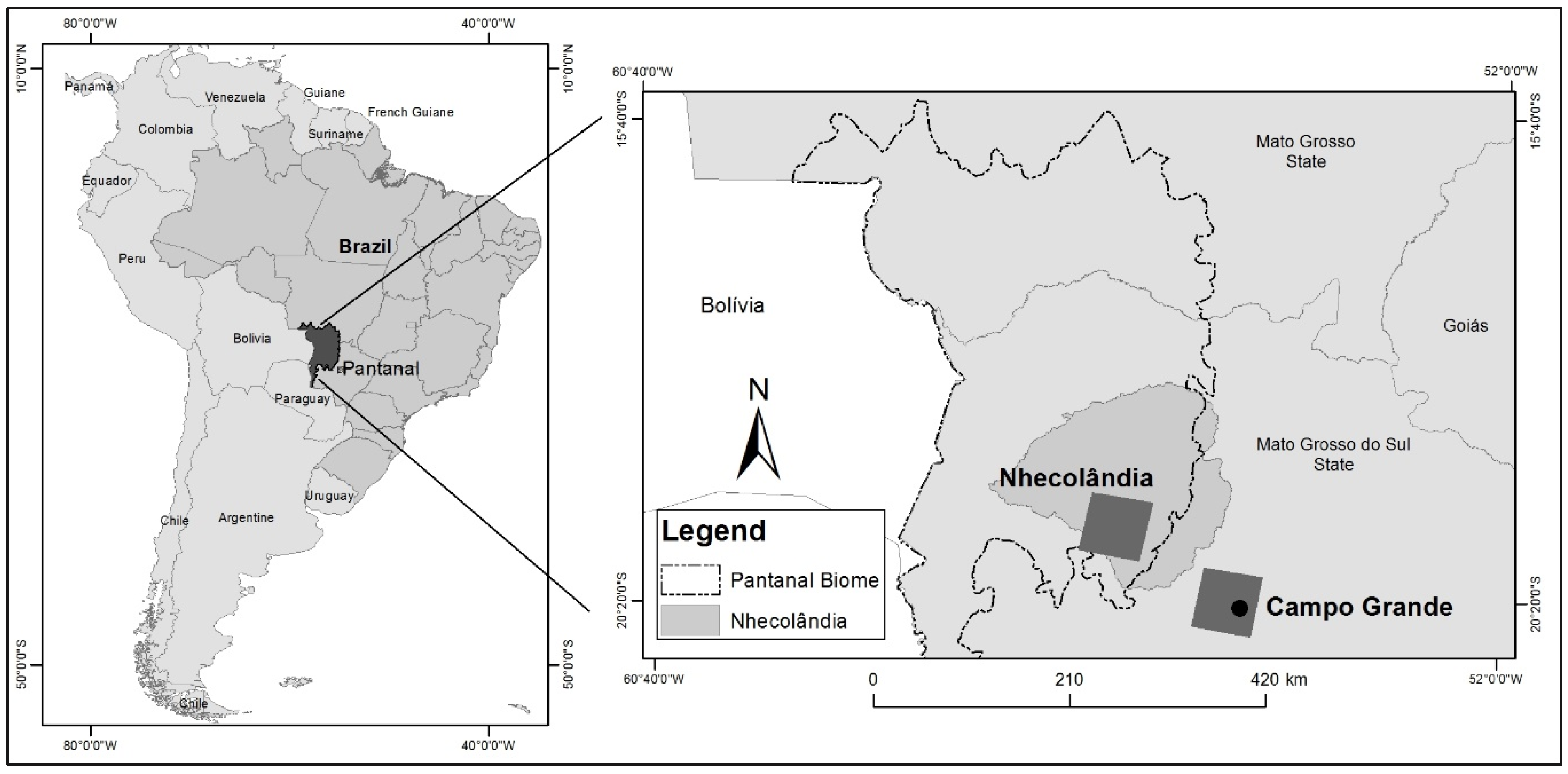
In this study, two areas were selected for the evaluation of downscaling methods of ASTER TIR images. The areas are located in the Brazilian Pantanal, comprising the regions of the city of Campo Grande located near the southern boundary of the Pantanal biome, and an area of natural seasonally flooded fields located in the Pantanal’s sub-region of Nhecolândia (Figure 1). The Pantanal wetlands of South America are one of the largest and most important tropical wetland ecosystems, covering an area of approximately 140,000 km2 during maximum inundation in the rainy season [47]. The rainfall patterns of the region support an annual flood regime that varies both temporally and spatially. Thus, the Pantanal wetland is composed of a number of floodplain sub-regions with particular biodiversity, hydrological, and geomorphological characteristics [48,49].
Given the high variability in environmental characteristics of this vast region [48,50,51,52,53,54], two areas with remarkably different patterns of land-cover/land-use (LCLU) were selected. The urban area of Campo Grande has been marked by an intense process of urbanization in the last decades, while in the Nhecolândia region the most remarkable features are thousands of small lakes/ponds composed of crystalline and salt waters [51], areas of natural vegetation (scrubs and grasslands), and scattered areas of pasture. Thus, these two areas were considered due to the high variety of anthropic features in the Campo Grande region and the remarkable nocturnal emissivity of the Pantanal saline lakes, easily observed in TIR satellite images acquired at night.
Some studies focused on hydrological processes require nighttime water emissivity data [51]. Therefore, the downscaling of ASTER data in the Nhecolândia region was carried out using ASTER scenes collected during the nighttime and the ancillary data (PAN bands) derived from 20-m SWIR and NIR bands of the Sentinel-2 satellite, acquired in March 2016. The Sentinel satellite was selected because it provided the acquisition period most close to the ASTER TIR acquisition, with a cloud-free scene within the studied area. The ASTER scenes were acquired in October 2014 and January 2016 for the Campo Grande and Nhecolândia regions, respectively. The downscaling of ASTER TIR data in the Campo Grande region was carried out using both TIR and VNIR channels of the same ASTER scene [35]. The Campo Grande region comprises an area of about 2570 km2, which corresponds to a subset of the original ASTER scene with dimensions of approximately 50 by 50 km. The Nhecolândia region covers an area of 2700 km2 with dimensions of 50 by 53 km.
The ASTER bands were provided by the USGS (United States Geological Survey) [55] at an L1T processing level, which comprises precision terrain corrected, registered at-sensor radiance. The VNIR and TIR products were provided as top of atmosphere (TOA) radiance (W m−2 sr−1 µm−1). The Sentinel-2 images were also provided in TOA radiance (W m−2 sr−1 µm−1) at an L1C processing level, which includes radiometric and geometric corrections comprising ortho-rectification and spatial registration on a global reference system (WGS 84) with sub-pixel accuracy [56]. Before merging the data, we carried out a correlation analysis between ancillary and TIR images of the studied areas, in order to select ancillary bands with correlation coefficients of up to 0.85. This analysis was necessary to avoid collinearity in the regression step of the GWRK and ATPRK fusion methods, which would increase computational time without adding any relevant information to the fused images. Thus, we selected the ancillary ASTER bands 1 and NDVI (r2: 0.72 between these two bands) for the Campo Grande region and the ancillary Sentinel-2 bands 8 and 11 for the Nhecolândia region (r2: 0.81 between these two bands).
3.2. Experimental Setup
The highest spatial resolution possible for both studied areas can be achieved by merging the 90-m ASTER TIR images with the 15-m ASTER VNIR bands or 20-m Sentinel bands to produce 15-m and 20-m TIR images in the Campo Grande and Nhecolândia regions, respectively. However, by adopting this strategy, no reference image would be available at the end of the process to assess the accuracy of the fusion methods. Given this, the merging process must be carried out by taking into account the availability of perfect fine spatial resolution reference images, which is achieved by degrading the original ASTER TIR, ASTER VNIR, and Sentinel images, while respecting the spatial resolution ratio of the images, as shown in Figure 2. The 90-m ASTER bands 13 and 14 were upscaled by factors of 6 and 4.5 for the Campo Grande and Nhecolandia regions, respectively, in order to generate merged images with a 90-m spatial resolution (Figure 2). The merging approaches were then implemented to merge the 540- and 405-m TIR bands with the 90-m ASTER VNIR and Sentinel-2 bands, which created images comparable to the reference 90-m TIR bands for the precise assessment of merging quality [35,57].
Following image downscaling, the ASTER TIR images were converted from radiance to surface LST. Image header parameters (conversion units) were used to convert digital numbers to at-sensor radiances. The thermal bands (TIR) 13 and 14 were calibrated to LST according to the method discussed by Jiménez-Muñoz [58]. The LST data retrieval from ASTER TIR bands is expected to be more accurate in the spectral region between 10 and 12 µm, which corresponds to bands 13 and 14. These bands show higher atmospheric transmissivity and, consequently, a good correlation with LST. Therefore, bands 13 and 14 were used for LST retrieval. The at-sensor radiances from bands 13 and 14 were converted to LST (Ts) according to the SCJM&S method detailed in Jiménez-Muñoz [58]. The final LST images represent the surface temperature in degrees Kelvin derived from bands 13 and 14. Both the reference and the merged images were converted in order to assess the quality of the downscaled images.
The three geostatistical methods, namely GWRK, ATPRK, and DCK, were compared to five state-of-the-art algorithms summarized in Vivone et al. [59] and Wang et al. [26]. They are ATWT, GS, MDMR, PCA, and TSHARP. Four indices were used for the quantitative evaluation of the spectral and spatial qualities of the LST downscaled bands 13 and 14, including the correlation coefficient (CC), relative global-dimensional synthesis error (ERGAS) [45], universal image quality index (UIQI) [60], and the spatial quality (SM) [61] index.
Given two images x and y, the CC is given as:
where and are the mean gray values of the reference and the fused bands, respectively, and CC is estimated globally for each LST image. The result of this equation shows similarities between the small structures of the original and fused images. The resulting values ranged from −1 to 1.
ERGAS (18) is an acronym in French for “Erreur relative globale adimensionnelle de synthese”, which translates to relative dimensionless global error in synthesis. This index is used to calculate the amount of spectral distortion between fused and reference images and is given by the following equation:
where h/l is the ratio between the spatial resolution of the panchromatic image and the MS image, N is the number of spectral bands of the fused image, µ0 is the mean value of each spectral band of the fused composition, and RMSE (relative root mean square error) represents the difference between the standard deviation and mean of the fused and original images. The best possible value for ERGAS is zero [45].
The UIQI (19,) proposed by Zhou and Bovik [60], considers the luminance, contrast, and structural differences between each band of the fused and original multispectral images, resulting in a global index representing the fusion quality.
where x and y are two non-negative image signals (gray values) for the fused and reference bands, respectively, while σxy, σx, and σy are the covariance and the variances of images x and y, respectively. The closer the UIQI index is to 1, the better the fused image.
The SM index is useful for evaluating the spatial quality of the downscaled images. The spatial features are extracted, by applying a Laplacian filter over all fused and reference LST images, prior to implementing the SM algorithm. The CC is then estimated for corresponding bands and the derived values are averaged, which results in an overall spatial measure. The SM index is mathematically expressed as follows:
where N is the total number of LST images, and CC represents the correlation coefficient obtained by (21):
where X and Y are the i-th bands in the reference and fused images, respectively, * is the convolution operator, and l is a Laplacian filter, set by Otazu et al. [61] as:
The SM values fall within a range of −1 to 1, where 1 indicates the best spatial quality.
Quantitative evaluation algorithms (17)–(20) result in a set of global quality indices for each fused LST band. Nevertheless, depending on the fusion algorithm, regional variations in fused bands might occur due to differences related to specific image features. Accordingly, the numerical expression of the fusion quality by means of a global value might lead to biased results, especially when considering fusion methods that cause a high standard deviation between the reference and fused bands. Given this, we adopted a regionalized approach by calculating the quality index within zonal moving windows (Figure 2) with dimensions 30 times greater than the resolution of the reference image (e.g., the zonal widow is a regular grid with dimensions of 2.7 by 2.7 km for the 90-m ASTER TIR images). The results of the quantitative approaches implemented for each fusion method were compared using descriptive statistics. The mean LST value of the downscaled TIR bands 13 and 14 were used for the quantitative evaluation of downscaling quality due to the very high spectral similarities between these two bands.
4. Results
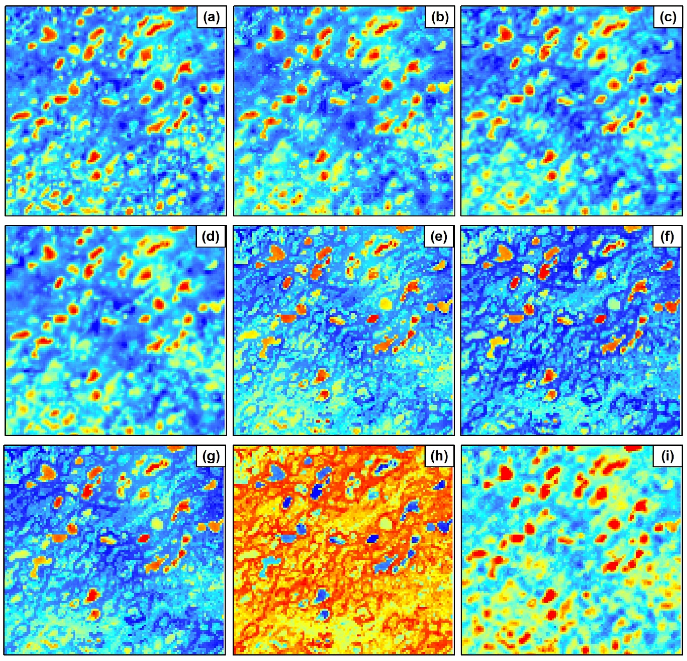
Figure 3 and Figure 4 summarize the image fusion results of the three geostatistical approaches (ATPRK, GWRK, and DCK) as well as the five other downscaling methods previously described, for the Campo Grande and Nhecolândia regions, respectively. The kriging methods ATPRK, DCK, and GWRK (Figure 4b–d) resulted in very similar temperature images when compared to the reference image (Figure 4a) in the Nhecolândia region. However, greater variability in temperature values was observed for the Campo Grande study area as a function of the different geostatistical approaches used (Figure 3b–d). As can be observed in Figure 3b, the ATPRK method caused a temperature overestimation in the urban area of Campo Grande, with some pixels showing reddish values in the central area of the city that are not visible in the reference image (Figure 3a). The ATPRK results showed a much higher contrast between low and high temperature values compared to the reference image (blue to red). While this effect was also observed in the image merged by DCK (Figure 3c), the scale had a lower contrast when compared to the ATPRK image (Figure 3b). The images merged by GWRK show a higher spectral similarity to the reference images of both studied areas (Figure 3d and Figure 4d).
Regarding to the non-geostatistical solutions, the image merged by TSHARP in Campo Grande (Figure 3i) presented the best results, when both the spatial and spectral coherence are considered. The ATWT (Figure 4e,g) and MDMR methods resulted in blurred images that masked the border features, thus causing a significant spectral mixture between the riparian forest at the center of the images (pattern of blue irregular lines) and the building zones of the city of Campo Grande (yellow to red patterns). In contrast, the images that most resembled the reference image in the Nhecolândia region were obtained using the ATWT (Figure 4e) and MDMR (Figure 4g) methods, followed by the GS method (Figure 4f). The poorest results for both areas were obtained by the PC method (Figure 3h and Figure 4h), which caused the complete inversion of temperature values in the Nhecolândia study area (Figure 4h) and saturation in the Campo Grande region (Figure 3h). Similar effects were also observed in the GS downscaled image of Campo Grande (Figure 3f).
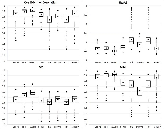
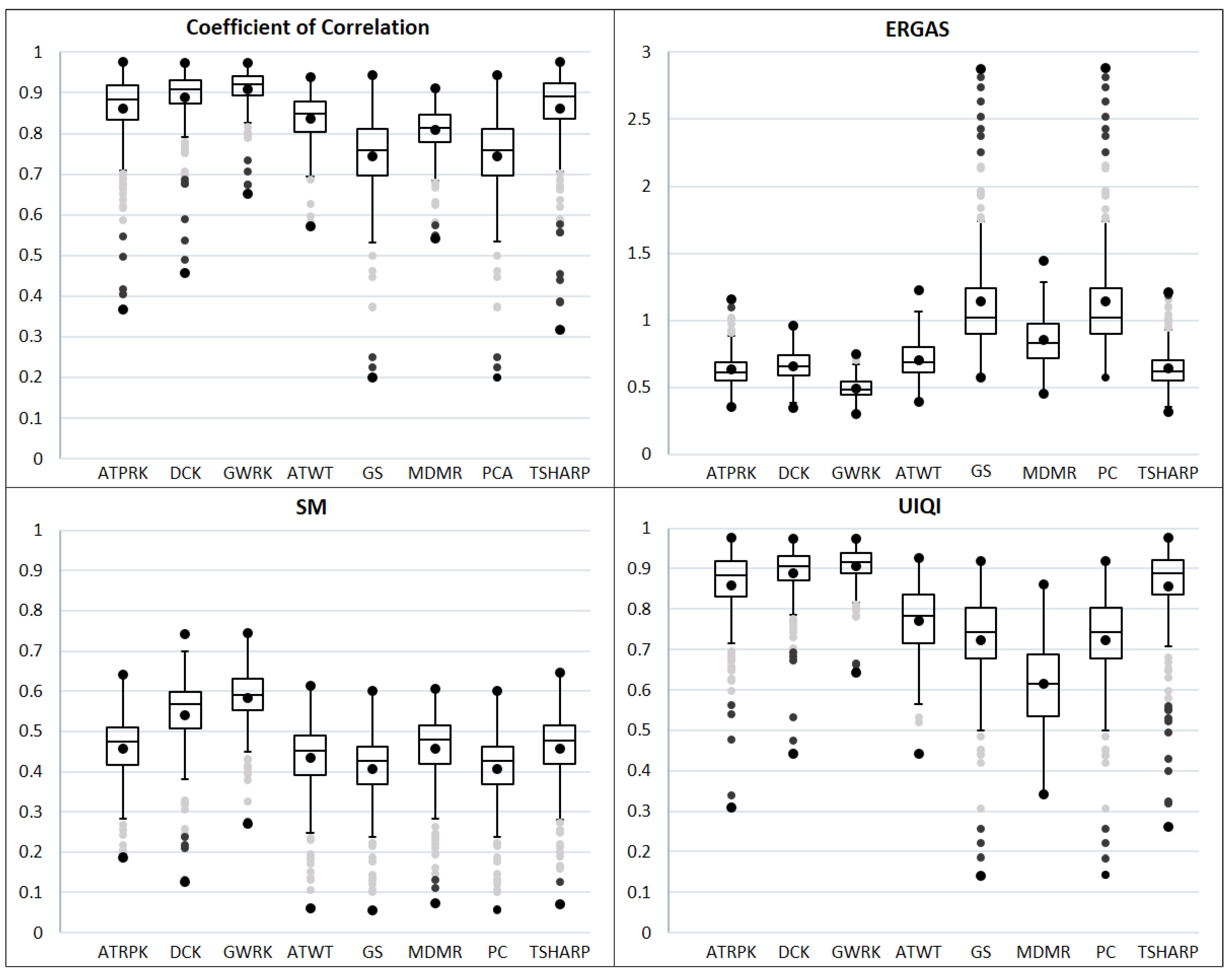
Figure 5 and Figure 6 show the quantitative evaluation of the downscaling methods for the Campo Grande and Nhecolândia study areas, respectively. The quantitative assessment, which was based on Equations (17)–(20), was carried out by assessing the correlation within a regular grid. As such, the results are expressed as the mean, median, quartiles, outliers, and extreme values (Figure 2). The ideal values of each index are provided at the top (CC, SM, and UIQI) and bottom (ERGAS) of the charts in order to facilitate the comparison of the fusion methods. With the exception of the TSHARP method that presented values close to those obtained by DCK, the three geostatistical approaches (ATPRK, DCK, and GWRK) outperformed the five state-of-the-art algorithms (Table 1 and Figure 5 and Figure 6). The CC, ERGAS, SM, and UIQI values of the GWRK were closer to the ideal values in all evaluated cases, considering both spectral (CC, ERGAS, UIQI) and spatial (SM) coherences. Moreover, the GWRK method resulted in fewer outliers and extreme values, due to its superior performance within all image targets of the fused TIR bands. If we compare, for example, ATPRK (the second-best method) and GWRK in the Campo Grande region (Figure 5), the CC and UIQI values are close (Table 1). However, there was a clear occurrence of extreme values and outliers in the ATPRK, with some values of CC and UIQI reaching 0.35. On the other hand, the extremely low values in the CC and UIQI for the GWRK were limited to 0.65, showing a better spectral coherence of this method within the entire merged image for the Campo Grande region (Figure 6).
The overall quality of merged images in the Campo Grande region (Figure 5) was higher when compared with the Nhecolândia region (Figure 6). No negative quality values were observed in the Campo Grande region for any of the fusion methods when using the CC, SM, and UIQI indices (Table 1). On the other hand, we observed a large number of negative values in Nhecolândia, mostly for the PC fusion method, with some negative outliers also related to the GS, MDMR, and ATWT methods (Figure 6). Despite the complex surface of the city of Campo Grande imparted by buildings and roads, the performance of the fusion methods was better due to a higher correlation between ancillary and TIR bands resulting from the images being collected by the same satellite platform (ASTER) in the same acquisition period. However, for the Nhecolândia region we used images from different satellites collected at different periods (day and night), which clearly caused a higher discrepancy between the reference and merged products (Figure 6). Moreover, the high nocturnal thermal emissivity of Nhecolândia lakes, typical of hyperalkaline water bodies [52], might cause an abnormal spectral response that is not observed in other satellite spectral bands, such as those in the VIS, NIR, and SWIR spectral ranges of the ASTER and Sentinel-2 satellites.
5. Discussion
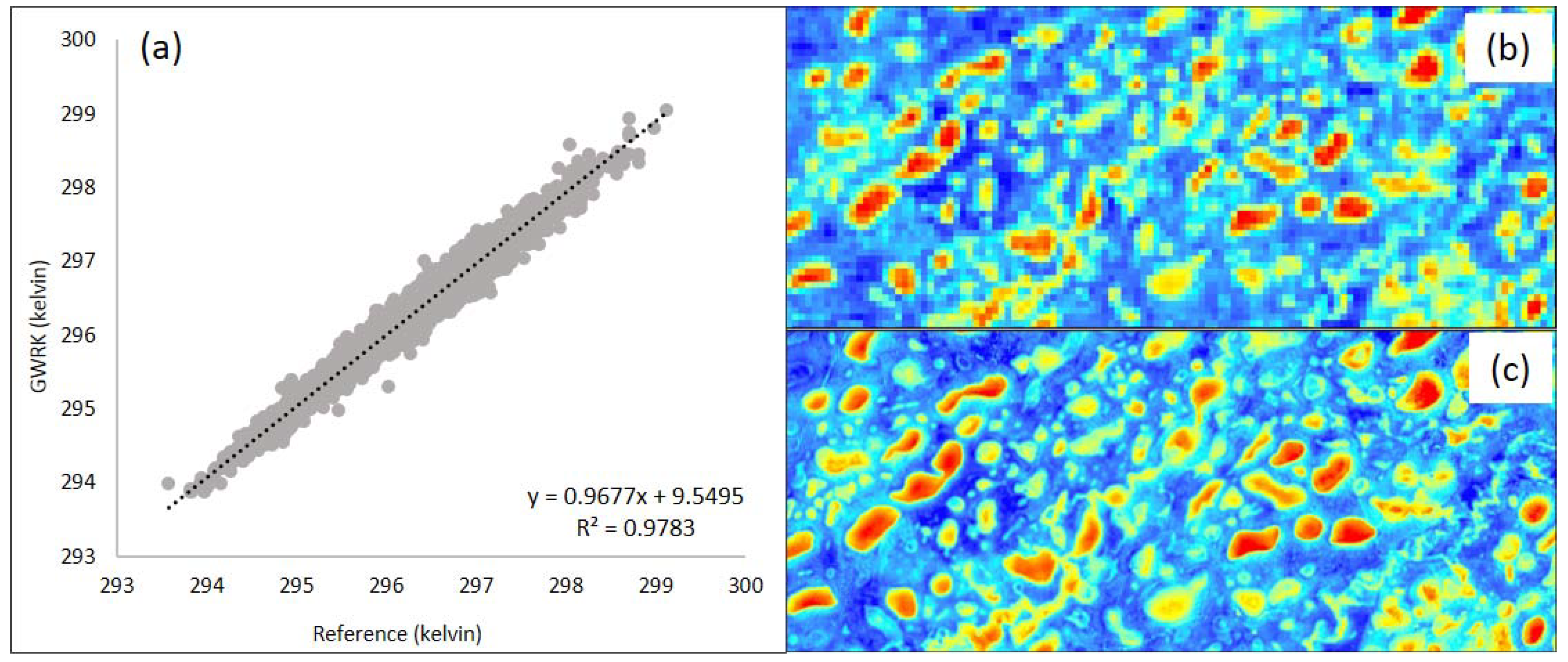
GWRK is similar to the AATPRK described by Wang et al. [26]. However, a distance-weighting scheme was also considered in this study. The authors highlighted the significant improvement in the quality of merged images resulting from the adoption of local windows, which was reflected in a coefficient of correlation close to 1 [26]. However, the authors did not consider distance-weighting schemes within the local regression windows. Therefore, the best method for refining ASTER temperature data without losing or distorting the original coarse information (Figure 7 and Figure 8), is to combine local regression windows, weighting distance schemes (Gaussian) within local windows, and a final area-to-point kriging of regressed residuals using multiple covariates (Figure 9). Moreover, the results are of higher quality when compared with other downscaling methods based on regression and kriging (GWK, ATPRK, and DCK), as well as the regression and interpolation of residuals (TSHARP). Further, the downscaling resulted in the generation of more ideal CC, ERGAS, SM, and UIQI values. Finally, the experiments demonstrated the great utility of using GWRK to merge data with high spectral sensibility. The results presented herein show great potential for estimating temperature at high spatial resolution, which can be useful when studying local phenomena, such as the occurrence of heat islands in dense urban areas (Figure 7) or evaluating nocturnal variability of water temperature (Figure 8) in flooded pristine regions.
It is important to highlight that the proposed GWRK method was compared to other state-of-the-art merging solutions based on kriging [13,35,42]. For the case of cokriging, we observed that the need to compute both the auto-semivariogram and the cross-semivariogram for each coarse band significantly increased the computational time, which made it impossible to use multiple covariates. On the other hand, GWRK and ATPRK are simpler and faster solutions since the mandatory process of cross-correlation between dependent and explanatory variables for kriging solutions is achieved by simply regressing the models globally (ATRPK) or locally with distance weighting (GWRK). Therefore, the kriging step of these methods, which calculates each coarse band separately, only requires the adjustment of the auto-semivariogram residuals for each coarse band, which was also observed by Wang et al. [28] for the ATRPK solution. As such, both ATPRK and GWRK are much faster to implement.
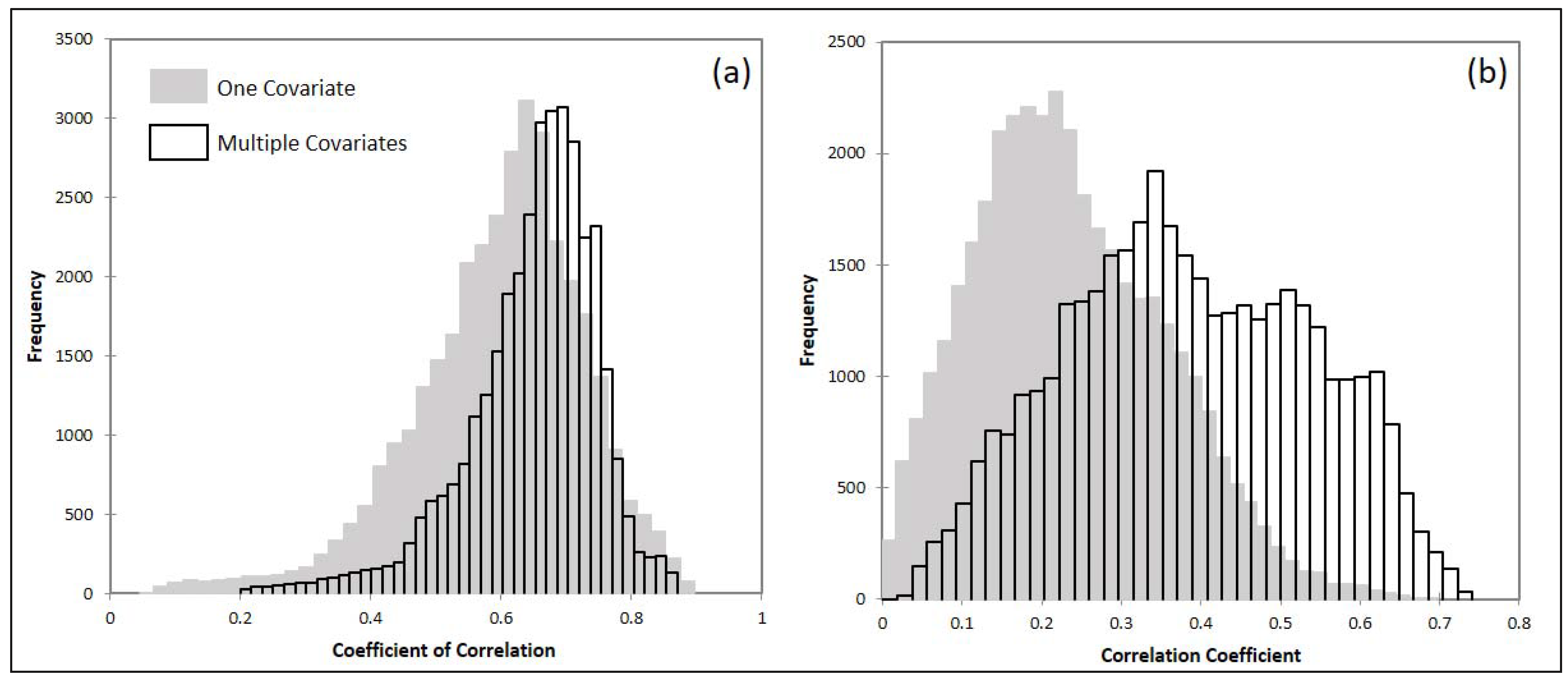
In order to improve the quality of the merged images, fusion methods with multiple explanatory panchromatic bands were tested (Figure 9). The ability to combine multiple covariates improved the quality of the methods based on regression (ATPRK and GWRK), as shown in Figure 9, which highlights the quality of the regressed surfaces using GWR prior to the kriging of the regressed residuals. The impact of multiple covariates on improving the quality of the merged images was clearer in the Nhecolândia region (Figure 9b) where GWR with just one covariate (Sentinel-2 band 12), resulting in a generally lower correlation within the local GWR windows. When using just one covariate (NDVI), the correlation values were higher in the Campo Grande region than in Nhecolândia. Further improvements were noted when multiple covariates were adopted for the Campo Grande region (Figure 9a); however, they were not as significant as in Nhecolândia (Figure 9b). Given this, it is advised to use multiple covariates when applying GWRK to merge images, since a significant improvement can be achieved, especially when working with panchromatic and multispectral bands with lower correlations, as is the case for the Nhecolândia region (Figure 9b).
Multiple covariates combined with GWRK provided the best results for downscaling temperature data either using images collected by the same sensor and period, which was the case of the Campo Grande area, or using images acquired by different sensor systems at different time periods (daytime or nighttime acquisitions), which was the case for the Nhecolândia region. Moreover, the combination of multiple covariates and GWRK demonstrated high performance over a range of different image targets, such as urban areas, areas of native vegetation and agriculture, as well as floodplain regions.
6. Conclusions
Nowadays, there are still a few remote sensing satellites equipped with thermal sensors that acquire imagery data at high spatial and temporal resolutions. A few exceptions include Landsat 8 TIR and ASTER TIRS sensors, which provide data at a 90-m spatial resolution. However, some studies require data at more refined spatial scales. Therefore, in this research a series of state-of-the-art pan-sharpening methods were tested and a fusion approach based on GWR and area-to-point kriging of residuals was presented. The proposed method incorporates multiple covariates that are regressed by GWR, and the resulting residuals are refined to the resolution of the covariate bands by kriging.
The evaluation of the quality of the merging methods was carried out in two different regions with a high variety of natural and anthropogenic features, for which images from different satellites and sensor systems were merged. Following quantitative and qualitative analyses of the resulting images, the following conclusions were drawn: (i) the proposed GWRK outperformed all of the other evaluated methods, followed by the ATRPK method. The better performance of the proposed method was confirmed by quantitative analysis carried within zonal windows. The zonal CC, ERGAS, SM, and UIQI quality indices indicated that the GWRK method had the best performance in all evaluated scenarios considering both studied regions of Campo Grande and Nhecolândia; (ii) the quantitative evaluation of fused images is more precise when calculated zonally, instead of using global evaluation schemes; (iii) the use of multiple covariates is advised due to the significant improvement observed in the regressed surface from GWR as compared to regression with a single covariate, especially in areas with low correlation between panchromatic and TIR data.
Acknowledgments
We would like to thank the Brazilian National Council for Scientific and Technological Development (CNPq) for a postdoctoral scholarship in the frame of the project (Project Number: 150168/2017-9). This work was funded by grants from the Research Support Foundation of the State of São Paulo (FAPESP), thematic project number (2016/14277-6). We also would like to thank the team behind the SAGA (System for Automated Geoscientific Analyses) platform and the fellows of the Remote Sensing Laboratory of the Polytechnic University of Madrid, who provided the code for MDMR and ATWT merging methods within IJFusion application.
Author Contributions
O.J.R.P. conceived, designed, and performed the study; analyzed the data; and wrote the paper. A.J.M. and C.R.M. assisted with the suggestion of the study area, coordination of the research funded by CNPQq and FAPESP and general orientation and review of the paper. Y.L. supported with insights on image downscaling, also helping on the suggestion of improvements in the first efforts of O.J.R.P. on downscaling satellite images.
Conflicts of Interest
The authors declare no conflict of interest.
References
- Anderson, M.C.; Kustas, W.P.; Norman, J.M.; Hain, C.R.; Mecikalski, J.R.; Schultz, L.; González-Dugo, M.P.; Cammalleri, C.; D’Urso, G.; Pimstein, A.; et al. Mapping daily evapotranspiration at field to continental scales using geostationary and polar orbiting satellite imagery. Hydrol. Earth Syst. Sci. 2011, 15, 223–239. [Google Scholar] [CrossRef] [Green Version]
- Trenberth, D. Climate System Modeling; Cambridge University Press: Cambridge, UK, 1992; ISBN 9780874216561. [Google Scholar]
- Carlson, T. An overview of the “triangle method” for estimating surface evapotranspiration and soil moisture from satellite imagery. Sensors 2007, 7, 1612–1629. [Google Scholar] [CrossRef]
- Gillies, R.R.; Carlson, T.N.; Cui, J.; Kustas, W.P.; Humes, K.S. A verification of the “triangle” method for obtaining surface soil water content and energy fluxes from remote measurements of the normalized difference vegetation index (NDVI) and surface e. Int. J. Remote Sens. 1997, 18, 3145–3166. [Google Scholar] [CrossRef]
- Moran, M. Thermal infrared measurement as an indicator of plant ecosystem health. Therm. Remote Sens. Land Surf. Process. 2004, 257–282. [Google Scholar] [CrossRef]
- Jin, M.; Dickinson, R.E.; Zhang, D.L. The footprint of urban areas on global climate as characterized by MODIS. J. Clim. 2005, 18, 1551–1565. [Google Scholar] [CrossRef]
- Weng, Q. Thermal infrared remote sensing for urban climate and environmental studies: Methods, applications, and trends. ISPRS J. Photogramm. Remote Sens. 2009, 64, 335–344. [Google Scholar] [CrossRef]
- Imhoff, M.L.; Zhang, P.; Wolfe, R.E.; Bounoua, L. Remote sensing of the urban heat island effect across biomes in the continental USA. Remote Sens. Environ. 2010, 114, 504–513. [Google Scholar] [CrossRef]
- Oke, T.R. The energetic basis of the urban heat island. Q. J. R. Meteorol. Soc. 1982, 108, 1–24. [Google Scholar] [CrossRef]
- Rajasekar, U.; Weng, Q. Spatio-temporal modelling and analysis of urban heat islands by using Landsat TM and ETM+ imagery. Int. J. Remote Sens. 2009, 30, 3531–3548. [Google Scholar] [CrossRef]
- Streutker, D.R. Satellite-measured growth of the urban heat island of Houston, Texas. Remote Sens. Environ. 2003, 85, 282–289. [Google Scholar] [CrossRef]
- Kustas, W.P.; Norman, J.M.; Anderson, M.C.; French, A.N. Estimating subpixel surface temperatures and energy fluxes from the vegetation index-radiometric temperature relationship. Remote Sens. Environ. 2003, 85, 429–440. [Google Scholar] [CrossRef]
- Pardo-Igúzquiza, E.; Chica-Olmo, M.; Atkinson, P.M. Downscaling cokriging for image sharpening. Remote Sens. Environ. 2006, 102, 86–98. [Google Scholar] [CrossRef]
- Liu, D.; Pu, R. Downscaling thermal infrared radiance for subpixel land surface temperature retrieval. Sensors 2008, 8, 2695–2706. [Google Scholar] [CrossRef] [PubMed]
- Agam, N.; Kustas, W.P.; Anderson, M.C.; Li, F.; Neale, C.M.U. A vegetation index based technique for spatial sharpening of thermal imagery. Remote Sens. Environ. 2007, 107, 545–558. [Google Scholar] [CrossRef]
- Jeganathan, C.; Hamm, N.A.S.; Mukherjee, S.; Atkinson, P.M.; Raju, P.L.N.; Dadhwal, V.K. Evaluating a thermal image sharpening model over a mixed agricultural landscape in India. Int. J. Appl. Earth Obs. Geoinf. 2011, 13, 178–191. [Google Scholar] [CrossRef]
- Tang, Y.; Atkinson, P.M.; Zhang, J. Downscaling remotely sensed imagery using area-to-point cokriging and multiple-point geostatistical simulation. ISPRS J. Photogramm. Remote Sens. 2015, 101, 174–185. [Google Scholar] [CrossRef]
- Merlin, O.; Duchemin, B.; Hagolle, O.; Jacob, F.; Coudert, B.; Chehbouni, G.; Dedieu, G.; Garatuza, J.; Kerr, Y. Disaggregation of MODIS surface temperature over an agricultural area using a time series of Formosat-2 images. Remote Sens. Environ. 2010, 114, 2500–2512. [Google Scholar] [CrossRef] [Green Version]
- Moran, M.S. A window-based technique for combining landsat thematic mapper thermal data with higher-resolution multispectral data over agricultural lands. Photogramm. Eng. Remote Sens. 1990, 56, 334–337. [Google Scholar]
- Zhukov, B.; Oertel, D.; Lanzl, F.; Reinhäckel, G. Unmixing-based multisensor multiresolution image fusion. IEEE Trans. Geosci. Remote Sens. 1999, 37, 1212–1226. [Google Scholar] [CrossRef]
- Fasbender, D.; Tuia, D.; Bogaert, P.; Kanevski, M. Support-based implementation of bayesian data fusion for spatial enhancement: Applications to ASTER thermal images. IEEE Geosci. Remote Sens. Lett. 2008, 5, 598–602. [Google Scholar] [CrossRef]
- Nichol, J. An Emissivity Modulation Method for Spatial Enhancement of Thermal Satellite Images in Urban Heat Island Analysis. Photogramm. Eng. Remote Sens. 2009, 75, 547–556. [Google Scholar] [CrossRef]
- Dominguez, A.; Kleissl, J.; Luvall, J.C.; Rickman, D.L. High-resolution urban thermal sharpener (HUTS). Remote Sens. Environ. 2011, 115, 1772–1780. [Google Scholar] [CrossRef]
- Zhan, W.; Chen, Y.; Zhou, J.; Li, J.; Liu, W. Sharpening thermal imageries: A generalized theoretical framework from an assimilation perspective. IEEE Trans. Geosci. Remote Sens. 2011, 49, 773–789. [Google Scholar] [CrossRef]
- Lee, J.; Lee, C. Fast and efficient panchromatic sharpening. IEEE Trans. Geosci. Remote Sens. 2010, 48, 155–163. [Google Scholar] [CrossRef]
- Wang, Q.; Shi, W.; Atkinson, P.M. Area-to-point regression kriging for pan-sharpening. ISPRS J. Photogramm. Remote Sens. 2016, 114, 151–165. [Google Scholar] [CrossRef]
- Ribeiro Sales, M.H.; Souza, C.M.; Kyriakidis, P.C. Fusion of MODIS images using kriging with external drift. IEEE Trans. Geosci. Remote Sens. 2013, 51, 2250–2259. [Google Scholar] [CrossRef]
- Wang, Q.; Shi, W.; Atkinson, P.M.; Zhao, Y. Downscaling MODIS images with area-to-point regression kriging. Remote Sens. Environ. 2015, 166, 191–204. [Google Scholar] [CrossRef]
- Vogel, R.L.; Privette, J.L.; Yu, N. Creating proxy VIIRS data from MODIS: Spectral transformations for mid- and thermal-infrared bands. IEEE Trans. Geosci. Remote Sens. 2008, 46, 3768–3782. [Google Scholar] [CrossRef]
- Szymanowski, M.; Kryza, M.; Spallek, W. Regression-based air temperature spatial prediction models: An example from Poland. Meteorol. Z. 2013, 22, 577–585. [Google Scholar] [CrossRef]
- Harris, P.; Fotheringham, A.S.; Crespo, R.; Charlton, M. The Use of Geographically Weighted Regression for Spatial Prediction: An Evaluation of Models Using Simulated Data Sets. Math. Geosci. 2010, 42, 657–680. [Google Scholar] [CrossRef]
- Stewart Fotheringham, A.; Charlton, M.; Brunsdon, C. The geography of parameter space: An investigation of spatial non-stationarity. Int. J. Geogr. Inf. Syst. 1996, 10, 605–627. [Google Scholar] [CrossRef]
- Fotheringham, A.S. Trends in quantitative methods I: Stressing the local. Prog. Hum. Geogr. 1997, 21, 88–96. [Google Scholar] [CrossRef]
- O’sullivan, D. Geographically Weighted Regression: The Analysis of Spatially Varying Relationships, by A. S. Fotheringham, C. Brunsdon, and M. Charlton. Geogr. Anal. 2003, 35, 272–275. [Google Scholar] [CrossRef]
- Rodriguez-Galiano, V.; Pardo-Iguzquiza, E.; Sanchez-Castillo, M.; Chica-Olmoa, M.; Chica-Rivas, M. Downscaling Landsat 7 ETM+ thermal imagery using land surface temperature and NDVI images. Int. J. Appl. Earth Obs. Geoinf. 2012, 18, 515–527. [Google Scholar] [CrossRef]
- Kim, S.; Kang, S.; Lee, K. Comparison of fusion methods for generating 250 m MODIS image. Korean J. Remote Sens. 2010, 26, 305–316. [Google Scholar]
- Kitanidis, P.K. Generalized covariance functions in estimation. Math. Geol. 1993, 25, 525–540. [Google Scholar] [CrossRef]
- Kyriakidis, P.C.; Yoo, E.H. Geostatistical prediction and simulation of point values from areal data. Geogr. Anal. 2005, 37, 124–151. [Google Scholar] [CrossRef]
- Kyriakidis, P.C. A geostatistical framework for area-to-point spatial interpolation. Geogr. Anal. 2004, 36, 259–289. [Google Scholar] [CrossRef]
- Atkinson, P.M. Downscaling in remote sensing. Int. J. Appl. Earth Obs. Geoinf. 2013, 22, 106–114. [Google Scholar] [CrossRef]
- Pardo-Iguzquiza, E.; Rodríguez-Galiano, V.F.; Chica-Olmo, M.; Atkinson, P.M. Image fusion by spatially adaptive filtering using downscaling cokriging. ISPRS J. Photogramm. Remote Sens. 2011, 66, 337–346. [Google Scholar] [CrossRef]
- Atkinson, P.M.; Pardo-Igúzquiza, E.; Chica-Olmo, M. Downscaling cokriging for super-resolution mapping of continua in remotely sensed images. IEEE Trans. Geosci. Remote Sens. 2008, 46, 573–580. [Google Scholar] [CrossRef]
- Chavez, P.S., Jr.; Sides, S.C.; Anderson, J.A. Comparison of three different methods to merge multiresolution and multispectral data: Landsat TM and SPOT panchromatic. Photogramm. Eng. Remote Sens. 1991, 57, 295–303. [Google Scholar]
- Laben, C.; Brower, B. Process for Enhancing the Spatial Resolution of Multispectral Imagery Using Pan-Sharpening. U.S. Patent 6,011,875, 4 January 2000. [Google Scholar]
- Ranchin, T.; Aiazzi, B.; Alparone, L.; Baronti, S.; Wald, L. Image fusion—The ARSIS concept and some successful implementation schemes. ISPRS J. Photogramm. Remote Sens. 2003, 58, 4–18. [Google Scholar] [CrossRef]
- Lillo-Saavedra, M.; Gonzalo, C.; Arquero, A.; Martinez, E. Fusion of multispectral and panchromatic satellite sensor imagery based on tailored filtering in the Fourier domain. Int. J. Remote Sens. 2005, 26, 1263–1268. [Google Scholar] [CrossRef]
- Junk, W.J.; Da Cunha, C.N.; Wantzen, K.M.; Petermann, P.; Strüssmann, C.; Marques, M.I.; Adis, J. Biodiversity and its conservation in the Pantanal of Mato Grosso, Brazil. Aquat. Sci. 2006, 68, 278–309. [Google Scholar] [CrossRef]
- Hamilton, S.K.; Sippel, S.J.; Melack, J.M. Comparison of inundation patterns among major South American floodplains. J. Geophys. Res. Atmos. 2002, 107. [Google Scholar] [CrossRef]
- Hamilton, S.K.; Sippel, S.J.; Melack, J.M. Inundation patterns in the Pantanal wetland of South America determined from passive microwave remote sensing. Arch. Hydrobiol. 1996, 137, 1–23. [Google Scholar] [CrossRef]
- Assine, M.L.; Soares, P.C. Quaternary of the Pantanal, west-central Brazil. Quat. Int. 2004, 114, 23–34. [Google Scholar] [CrossRef]
- Barbiéro, L.; Queiroz Neto, J.P.; Ciornei, G.; Sakamoto, A.Y.; Capellari, B.; Fernandes, E.; Valles, V. Geochemistry of water and ground water in the Nhecolândia, Pantanal of Mato Grosso, Brazil: Variability and associated processes. Wetlands 2002, 22, 528–540. [Google Scholar] [CrossRef]
- Barbiero, L.; Filho, A.R.; Furquim, S.A.C.; Furian, S.; Sakamoto, A.Y.; Valles, V.; Graham, R.C.; Fort, M.; Ferreira, R.P.D.; Neto, J.P.Q. Soil morphological control on saline and freshwater lake hydrogeochemistry in the Pantanal of Nhecolândia, Brazil. Geoderma 2008, 148, 91–106. [Google Scholar] [CrossRef] [Green Version]
- De Almeida, T.I.R.; Fernandes, E.; Mendes, D.; Branco, F.C.; Sígolo, J.B. Distribuição espacial de diferentes classes de lagoas no pantanal da nhecolândia, MS, a partir de dados vetoriais e SRTM: Uma contribuição ao estudo de sua compartimentação e gênese. Geol. USP Ser. Cient. 2007, 7, 95–107. [Google Scholar] [CrossRef]
- Evans, T.L.; Costa, M. Landcover classification of the Lower Nhecolândia subregion of the Brazilian Pantanal Wetlands using ALOS/PALSAR, RADARSAT-2 and ENVISAT/ASAR imagery. Remote Sens. Environ. 2013, 128, 118–137. [Google Scholar] [CrossRef]
- USGS Earth Resources Observation and Science—EROS Center. Available online: http://eros.usgs.gov/ (accessed on 1 March 2016).
- ESA: European Space Agency Sentinels Scientific Data Hub. Available online: https://scihub.esa.int/ (accessed on 1 May 2016).
- Wald, L.; Ranchin, T.; Mangolini, M. Fusion of satellite images of different spatial resolutions : Assessing the quality of resulting images. Photogramm. Eng. Remote Sens. 1997, 63, 691–699. [Google Scholar]
- Jiménez-Muñoz, J.C.; Sobrino, J.A. A generalized single-channel method for retrieving land surface temperature from remote sensing data. J. Geophys. Res. 2003, 108. [Google Scholar] [CrossRef]
- Vivone, G.; Alparone, L.; Chanussot, J.; Dalla Mura, M.; Garzelli, A.; Licciardi, G.A.; Restaino, R.; Wald, L. A critical comparison among pansharpening algorithms. IEEE Trans. Geosci. Remote Sens. 2015, 53, 2565–2586. [Google Scholar] [CrossRef]
- Zhou, W.; Bovik, A.C. A universal image quality index. Sign. Process. Lett. IEEE 2002, 9, 81–84. [Google Scholar] [CrossRef]
- Otazu, X.; González-Audícana, M.; Fors, O.; Núñez, J. Introduction of Sensor Spectral Response into Image Fusion Methods. Application to Wavelet-Based Methods. IEEE Trans. Geosci. Remote Sens. 2005, 43, 2376–2385. [Google Scholar] [CrossRef] [Green Version]
Figure 1.
Study area in the context of the Brazilian portion of the Pantanal biome.

Figure 2.
Flowchart of the methodology applied to evaluate the quality of the land surface temperature (LST) downscaled image according to the different downscaling methods adopted in this study.
Figure 2.
Flowchart of the methodology applied to evaluate the quality of the land surface temperature (LST) downscaled image according to the different downscaling methods adopted in this study.

Figure 3.
Visual results of the merged images at a 90-m spatial resolution in a sector of the Campo Grande study area. The reference (a) image (mean of ASTER bands 13 and 14) as compared to the following methods: (b) ATPRK (Area-To-Point Regression Kriging); (c) DCK (Downscaling Cokriging); (d) GWRK (Geographically Weighted Regression Kriging); (e) ATWT (“À Trous” Wavelet Transform); (f) GS (Gram-Schmidt); (g) MDMR (MultiDirection-MultiResolution); (h) PCA (Principal Component Analysis); and (i) TSHARP.
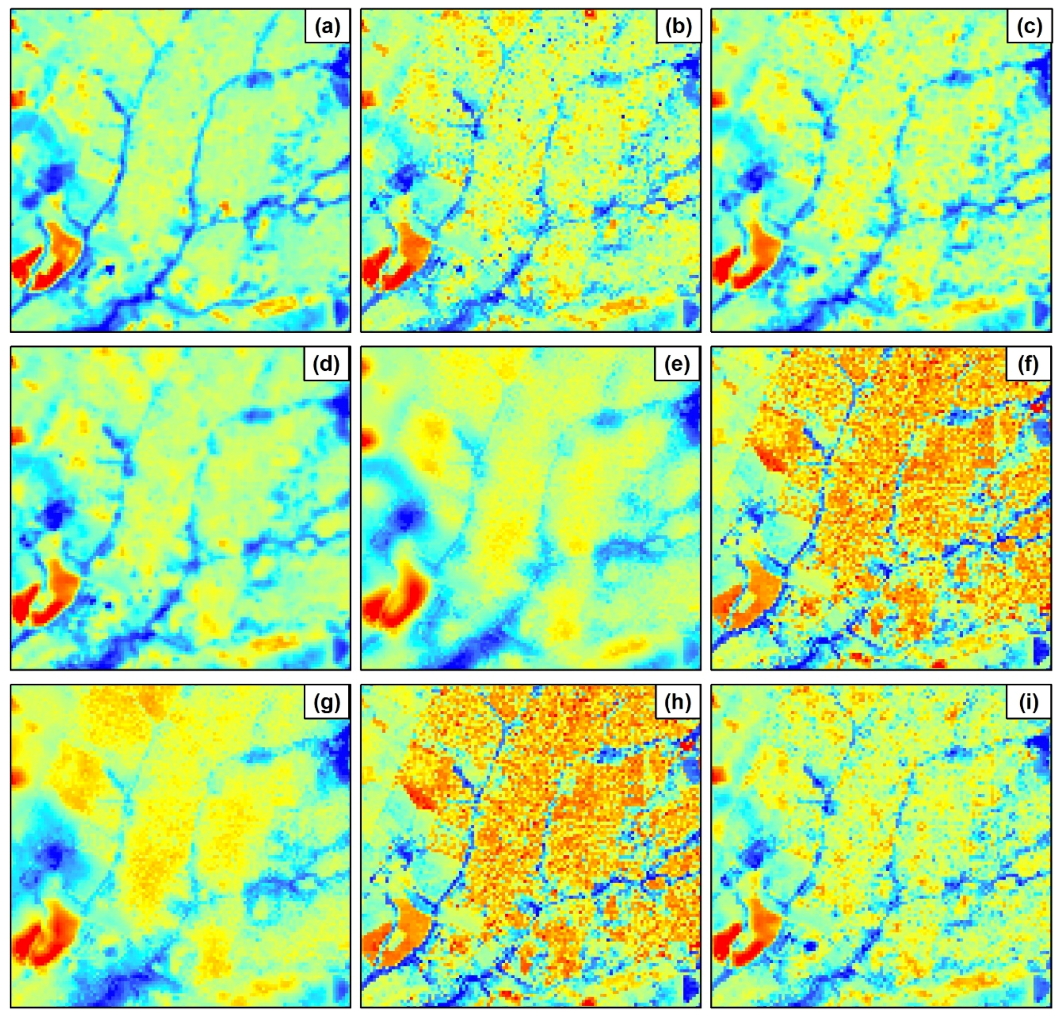
Figure 4.
Visual results of the merged images at a 90-m spatial resolution in a sector of the Nhecolândia study area. The reference (a) image (mean of ASTER bands 13 and 14) as compared to the following methods: (b) ATPRK; (c) DCK; (d) GWRK; (e) ATWT; (f) GS; (g) MDMR; (h) PCA; and (i) TSHARP.
Figure 4.
Visual results of the merged images at a 90-m spatial resolution in a sector of the Nhecolândia study area. The reference (a) image (mean of ASTER bands 13 and 14) as compared to the following methods: (b) ATPRK; (c) DCK; (d) GWRK; (e) ATWT; (f) GS; (g) MDMR; (h) PCA; and (i) TSHARP.

Figure 5.
Box-plots showing the fusion quality values for the Campo Grande region.

Figure 6.
Box-plots showing the merging quality values for the Nheoclândia region.
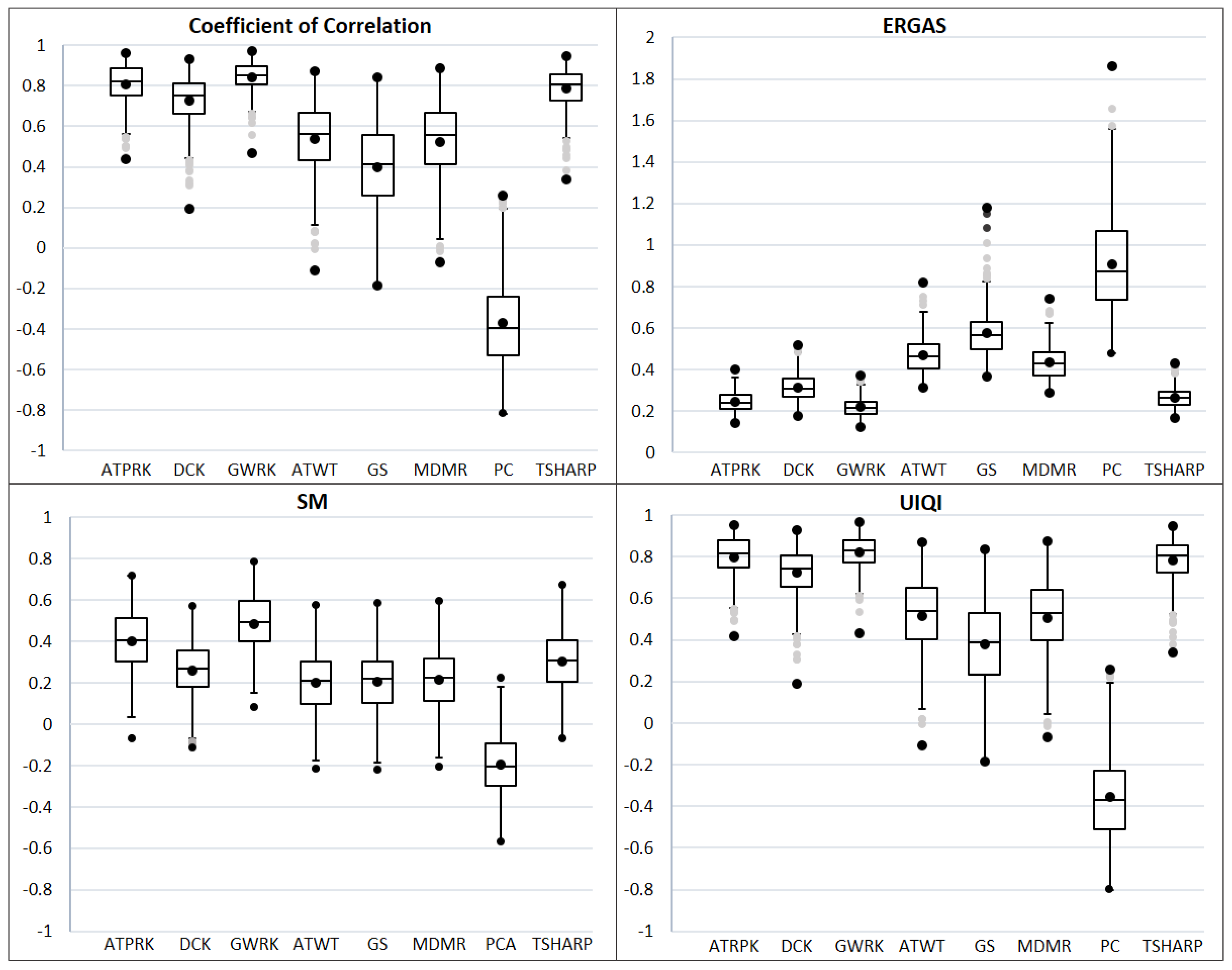
Figure 7.
Results of GWRK pan-sharpening for the Campo Grande study area: (a) Pixel-based comparison between the original 90-m TIR ASTER bands (mean of bands 13 and 14) and the merged GWRK image obtained from the degraded TIR and VNIR ASTER bands; (b) original TIR ASTER band; (c) result of GWRK pan-sharpening of TIR bands without degradation with a 15-m spatial resolution. Lower and higher temperatures range from blue to red, respectively.

Figure 8.
Results of GWRK pan-sharpening for the Nhecolândia study area: (a) Pixel-based comparison between the original 90-m TIR ASTER band (mean bands 13 and 14) and the merged GWRK image obtained from the degraded TIR and Sentinel-2 bands; (b) original TIR ASTER; (c) result of GWRK pan-sharpening of TIR bands without degradation, with a 20-m spatial resolution. Lower and higher temperatures range from blue to red, respectively.

Figure 9.
Results of GWR (Geographically Weighted Regression) with one and multiple covariates. Frequency distribution of the coefficient of correlation of the surfaces regressed by GWR (ancillary and TIR) within each local window without kriging in the (a) Campo Grande and (b) Nhecolândia study areas.


Table 1.
Quantitative assessment of the pan-sharpening methods. Average values of the zonal grid.
| CC | ERGAS | SM | UIQI | |||||
|---|---|---|---|---|---|---|---|---|
| Region | CG * | Nhe ** | CG | Nhe | CG | Nhe | CG | Nhe |
| GWRK | 0.91 | 0.84 | 0.49 | 0.22 | 0.58 | 0.49 | 0.91 | 0.82 |
| DCK | 0.89 | 0.81 | 0.66 | 0.25 | 0.54 | 0.40 | 0.89 | 0.80 |
| ATPRK | 0.86 | 0.78 | 0.64 | 0.26 | 0.46 | 0.31 | 0.86 | 0.78 |
| TSHARP | 0.86 | 0.73 | 0.64 | 0.31 | 0.46 | 0.26 | 0.86 | 0.72 |
| ATWT | 0.84 | 0.54 | 0.70 | 0.47 | 0.43 | 0.20 | 0.77 | 0.51 |
| MDMR | 0.81 | 0.52 | 0.85 | 0.43 | 0.46 | 0.21 | 0.61 | 0.51 |
| GS | 0.74 | 0.40 | 1.14 | 0.58 | 0.41 | 0.20 | 0.72 | 0.38 |
| PCA | 0.74 | −0.37 | 1.14 | 0.91 | 0.41 | −0.20 | 0.72 | −0.35 |
* CG: Campo Grande; ** Nhe: Nhecolândia.
© 2018 by the authors. Licensee MDPI, Basel, Switzerland. This article is an open access article distributed under the terms and conditions of the Creative Commons Attribution (CC BY) license (http://creativecommons.org/licenses/by/4.0/).
Share and Cite
MDPI and ACS Style
Pereira, O.J.R.; Melfi, A.J.; Montes, C.R.; Lucas, Y. Downscaling of ASTER Thermal Images Based on Geographically Weighted Regression Kriging. Remote Sens. 2018, 10, 633. https://doi.org/10.3390/rs10040633
AMA Style
Pereira OJR, Melfi AJ, Montes CR, Lucas Y. Downscaling of ASTER Thermal Images Based on Geographically Weighted Regression Kriging. Remote Sensing. 2018; 10(4):633. https://doi.org/10.3390/rs10040633
Chicago/Turabian StylePereira, Osvaldo José Ribeiro, Adolpho José Melfi, Célia Regina Montes, and Yves Lucas. 2018. "Downscaling of ASTER Thermal Images Based on Geographically Weighted Regression Kriging" Remote Sensing 10, no. 4: 633. https://doi.org/10.3390/rs10040633
Note that from the first issue of 2016, this journal uses article numbers instead of page numbers. See further details here.