Estimating Ocean Vector Winds and Currents Using a Ka-Band Pencil-Beam Doppler Scatterometer

Abstract

Ocean surface currents and winds are tightly coupled essential climate variables, and, given their short time scales, observing them at the same time and resolution is of great interest. DopplerScatt is an airborne Ka-band scatterometer that has been developed under NASA’s Instrument Incubator Program (IIP) to provide a proof of concept of the feasability of measuring these variables using pencil-beam scanning Doppler scatterometry. In the first half of this paper, we present the Doppler scatterometer measurement and processing principles, paying particular attention to deriving a complete measurement error budget. Although Doppler radars have been used for the estimation of surface currents, pencil-beam Doppler Scatterometry offers challenges and opportunities that require separate treatment. The calibration of the Doppler measurement to remove platform and instrument biases has been a traditional challenge for Doppler systems, and we introduce several new techniques to mitigate these errors when conical scanning is used. The use of Ka-band for airborne Doppler scatterometry measurements is also new, and, in the second half of the paper, we examine the phenomenology of the mapping from radar cross section and radial velocity measurements to winds and surface currents. To this end, we present new Ka-band Geophysical Model Functions (GMFs) for winds and surface currents obtained from multiple airborne campaigns. We find that the wind Ka-band GMF exhibits similar dependence on wind speed as that for Ku-band scatterometers, such as QuikSCAT, albeit with much greater upwind-crosswind modulation. The surface current GMF at Ka-band is significantly different from that at C-band, and, above 4.5 m/s has a weak dependence on wind speed, although still dependent on wind direction. We examine the effects of Bragg-wave modulation by long waves through a Modululation Transfer Function (MTF), and show that the observed surface current dependence on winds is consistent with past Ka-band MTF observations. Finally, we provide a preliminary validation of our geophysical retrievals, which will be expanded in subsequent publications. Our results indicate that Ka-band Doppler scatterometry could be a feasible method for wide-swath simultaneous measurements of winds and currents from space.

1. Introduction

The two-way interaction between ocean surface currents and ocean winds is an important component of the ocean-atmosphere system. Surface winds drive currents, but are, in their turn, modulated by currents since the forcing wind stress is relative to the current’s moving reference frame [1]. In addition, surface currents advect warm or cold water, and the resulting temperature gradients modulate the winds (e.g., [2]), possibly causing a change in the structure of mesoscale and sub-mesoscale circulation (e.g., [3]). At small space and time scales, the interaction of winds and surface currents becomes tighter as winds can drive inertial oscillations or aid in the formation of mesoscale fronts (e.g., [4]), where significant vertical ocean motion can occur, leading to enhanced mixing. For these reasons, it is very desirable to be able to obtain simultaneous synoptic measurements of ocean surface currents and winds.

Measurements of ocean vector winds have a long heritage with radar scatterometers using either Ku-band rotating pencil beam scatterometry (e.g., NASA’s Quick Scatterometer (QuikSCAT) and RapidScat, the Indian Space Research Organisation’s (ISRO) OSCAT and ScatSat) or multiple beam C-band scatterometry (e.g., EUMETSAT’s ASCAT series). The possibility of measuring surface currents using radar along-track interferometry was first suggested by Goldstein et al. [5,6] and an airborne vector measurement was demonstrated by [7]. Implementing a dual beam along-track interferometer from space is challenging. Chapron et al. [8], with colleagues from Institut français de recherche pour l’exploitation de la mer (IFREMER) and elsewhere, suggested that single-antenna Synthetic Aperture Radar (SAR) Doppler centroid measurements could be used instead, albeit potentially at lower resolution and accuracy. Rodríguez (Ocean Vector Winds Science Team Meeting, 2012) suggested that a slight modification of the pencil beam scatterometer to include Doppler measurements could produce wide-swath vector surface current measurements, and Bao et al. [9] subsequently published an analysis of the performance of a Doppler scatterometer spaceborne system. Fois et al. [10] showed that a Doppler system amenable to the ASCAT architecture could also be implemented by correlating the Doppler shift from opposite sense linear frequency modulated pulses (i.e., chirps).

Given the scientific potential for simultaneous measurements of winds and currents, NASA funded the development of a Ka-band Doppler scatterometer system, called DopplerScatt, under the NASA Instrument Incubator Program (IIP). Here, we present the Ka-band measurement phenomenology, the processing and calibration algorithms, and the detailed measurement error budget for the DopplerScatt wind and current measurements. These measurements are then validated using data collected in several field campaigns.

The DopplerScatt instrument design is presented in Section 2.1. We then present a review of the measurement principles and an overview of the processing in Section 2.2. The measurement principles are examined further in Appendix A, which extends the work of Bao et al. [9] to include several additional effects. One aspect where pencil-beam Doppler centroid systems differ from side-looking SAR systems is in the variation of Doppler bandwidth with scan angle [11]. This variation allows the estimation of the Doppler centroid using phases from multiple bursts in order to reduce the noise of the estimate. We present detailed algorithms for the estimation of the Doppler centroid that extend the classical work of Madsen [12] to multiple bursts in Section 2.5. We derive a new analytical estimate for the radial velocity and validate it using DopplerScatt field measurements.

In Section 2.4, Section 2.5 and Section 2.6, we present the description of the end-to-end processing algorithms. Given the novelty of the pencil-bean Doppler measurements, we pay attention to the sensitivity equations for the velocity, and validate the DopplerScatt random error performance by comparing theoretical predictions and estimates obtained from campaign data.

DopplerScatt also differs from spaceborne scatterometers in having only one polarization and one antenna beam. In traditional scatterometry, this limitation would lead to unacceptable azimuth ambiguities, but we show in Section 2.6 that, following the spirit of Mouche et al. [13], the surface current radial velocity information can be used to obtain unambiguous wind directions.

A critical part of the radial velocity measurement (and one of the primary limitations for spaceborne SAR systems to date) is calibrating the antenna position so that the look vector is known to sufficient accuracy. In Section 2.8, we show that it is possible to use measurements over multiple scan cycles of the pencil-beam antenna to determine angular biases and illustrate with results from DopplerScatt. These results illustrate the system’s stability over multiple campaigns.

After laying down the theoretical and processing framework, we examine in Section 3 the geophysical results obtained during multiple flights conducted by the DopplerScatt instrument during 2016 and 2017. These results include estimates of the ocean correlation times at Ka-band (Section 3.1); estimates of the geophysical model function (GMF) relating ${\sigma }_0$ and winds for vertical-polarization, moderate incidence angle Ka-band data (Section 3.2); the separation of the ocean surface currents into two components: one directly proportional to the local wind, representing the sum of Bragg wave motion, Stokes and wind drift, and coupling of surface waves orbital velocities; and another one corresponding to the deeper current that does not respond immediately to the local wind (Section 3.4). In Section 3.3, Section 3.4 and Section 3.5, we present some preliminary comparisons of the final DopplerScatt data products against available in situ data. Given the complexity of comparing radar surface velocities with in situ measurements conducted by various methods, we will give a more detailed accounting of this subject elsewhere. The mechanisms that generate the surface current GMF through modulation of Bragg waves by long ocean waves are discussed in Section 4. Finally, in Section 4 and Section 5, we compare our findings with similar findings obtained at different frequencies or by different measurements, and assess the prospects for Ka-band Doppler scatterometry.

2. Materials and Methods

2.1. The DopplerScatt Instrument

DopplerScatt is a vertically polarized single-beam Ka-band coherent scatterometer using a rotating pencil-beam antenna to illuminate circular regions that can be built into a continuous swath, similar to the principle of the NASA’s Seawinds Instrument on QuikSCAT [14]. The 12 RPM rotation rate of the antenna is set so that, for a given range, every point in the swath is observed from at least two different directions, resulting in the observation geometry shown in Figure 1. The data are recorded coherently onboard and processed on the ground to estimate radial velocities, by using pulse-pair phase differences, and normalized radar backscatter cross sections, ${\sigma }_0$. The azimuth diversity of the measurements allows for inversion of both vector surface velocities and winds, as will be explained below. The antenna beam boresight is set at a nominal incidence angle of ${56}^{°}$, which, at a nominal flight altitude of 8.53 km, results in a ground scan radius, R, of approximately 12.5 km, for a total observation swath of about 25 km. The system is highly configurable in terms of the inter-pulse period, the burst repetition interval, and the system bandwidth, allowing for operation at multiple altitudes.

Table 1. DopplerScatt nominal parameters.

Parameter	Value
Peak Power	100 W
3 dB Azimuth Beamwidth	$3^{°}$
3 dB Azimuth Footprint	600 m
3 dB Elevation Beamwidth	$3^{°}$
3 dB Elevation Footprint	1.4 km
Nominal boresight angle	${56}^{°}$
Burst Repetition Frequency	4.5 kHz
Inter-pulse Period	18.4 $\mathsf{\mu }$s
Chirp length	6.4 $\mathsf{\mu }$s
Pulses per burst	4
Pulse Bandwidth	5 MHz
Azimuth Looks	100
Range Resolution	30 m
Resolution in Elevation	36.2 m
Resolution in Azimuth	485 m
Nominal Platform Altitude	8.53 km
Nominal Swath	25 km
Scan Rate	12 RPM
Noise Equivalent ${\sigma }_0$	−37 dB

presents the configuration that was used to obtain the results used in this paper.

A 3D model of DopplerScatt is presented in Figure 2. A 5 MHz chirp signal is generated digitally, upconverted, and amplified using a commercial Ka-band solid state amplifier (SSPA), built by QuinStar Technology (Torrance, CA, USA), to achieve a peak transmit power of 100 W. The signal is transmitted and received by a rotating, $3^{°}$ one-way beamwidth, vertically-polarized, waveguide slotted array antenna, base-banded by the Radio-Frequency (RF) receiver, and digitized at a high rate by a commercial digital receiver built by Remote Sensing Solutions (Barnstable, MA, USA). The processing of the complex data from the digital receiver will be described below. For the nominal system parameters in Table 1, the system achieves a noise-equivalent ${\sigma }_0$ of about −37 dB, which is sufficient for sampling scenes for even very low winds ($\mathcal{O}$ (2 m/s)).

Although the system pulse repetition frequency allows for SAR processing, the achievable azimuth resolution using SAR will vary significantly with azimuth angle, and, at this point, we have decided to process the data in real-aperture mode to obtain more uniform sampling characteristics. This leads to a two-way azimuth footprint size of approximately 600 m. In the range direction, the chirp bandwidth results in a ground sample spacing of 36 m. The achievable ground resolution when combining measurements from different azimuth directions will vary across the swath, but the combination of partially overlapping skewed footprints can lead to significant improvements in the resolution cell size since the areas of overlap are emphasized, especially in the swath “sweet-spots” between the nadir track and the far-swath (see, e.g., [15]).

Pulsed pair Doppler processing is achieved by cross-correlating bursts, which are transmitted at a burst repetition frequency of 4.5 kHz, Nyquist oversampling the Doppler bandwidth for all azimuth angles. The system’s phase and power stability is monitored using an internal calibration loop which includes the transmit and receive paths, excluding the rotating antenna. Intensive laboratory testing prior to deployment, and subsequent calibration field data, showed that the pulse-pair difference timing stability is insensitive to temperature and introduces radial velocity errors much smaller than 1 cm/s. The system delay showed some sensitivity to temperature, but drifts were much smaller than the inverse bandwidth of the system. The system gain exhibited variations with temperature and these were calibrated using loop-back calibration and corrected during the processing to obtain ${\sigma }_0$.

The instrument position and attitude are obtained using a GPS receiver coupled with an Applanix POS AV-610 Internal Motion Unit (IMU) (Richmond Hill, Canada). The IMU manufacturer specifications relevant to DopplerScatt’s performance are given in

Table 2. Applanix POS AV 610 performance specifications.

Parameter	Accuracy
True Heading	5 mdeg
Roll & Pitch	2.5 mdeg
Attitude Drift	<0.01 deg/h
Velocity	0.5 cm/s
Horizontal Position	<10 cm
Vertical Position	<20 cm

, assuming Precise Point Positioning (PPP) processing. The rotation angle is obtained by means of an encoder, which has a nominal resolution of 88 mdeg, but has an unknown mounting offset that needs to be obtained from calibration. The nominal antenna pattern was obtained using near-range field measurements. The nominal boresight was obtained by combining mechanical measurements of the antenna location together with IMU attitudes and the azimuth encoder measurement.

2.2. Current Measurement Principle

DopplerScatt measures two basic quantities, pulse-pair phase differences and return power, which are then converted to surface radial velocities, $v_{rS}$, and normalized backscatter cross section, ${\sigma }_0$. The use of ${\sigma }_0$ for vector wind retrieval using a pencil-beam scatterometer is well known (e.g., [16]), and we refer the reader to the literature for a review of the principles. The principles of using a pencil-beam system to measure surface currents was presented by Bao et al. [9]. In this paper, we extend their derivation to include various effects not accounted for in their first order approximation and also examine the algorithm for radial velocity in detail.

In Appendix A, we present a detailed measurement model and find that the complex correlation coefficient, $\gamma \left(\tau \right)$, for a pulse pair separated by a time $\tau$ is given by

$$\begin{array}{cc}\hfill \frac{〈E_1{E}_2^{*}〉}{\sqrt{〈{\left|E_1\right|}^2〉〈{\left|E_2\right|}^2〉}}& \equiv \gamma \left(\tau \right)=\exp \left[-i\Phi \left(\tau \right)\right]{\gamma }_N{\gamma }_T\left(\tau \right)\left|{\gamma }_D\left(\tau \right)\right|,\hfill \end{array}$$

(1)

$$\begin{array}{cc}\hfill \frac{\Phi }{2k\tau }& =\widehat{\ell }·\left({\mathbf{v}}_p-\left({\mathbf{v}}_W+{〈\frac{\delta {\sigma }_0}{{\sigma }_0}\widehat{\ell }·\delta {\mathbf{v}}_W〉}_W\right)\right)-v_{rG}-v_{rA},\hfill \end{array}$$

(2)

where $E_i$ is the complex return signal, $\Phi$ is the pulse-pair phase difference, $2k\tau =4\pi \tau /\lambda$, $\widehat{\ell }$ is the look vector from the platform to the scattering cell (we drop the C subscript and overbars of Appendix A in the main text to simplify notation), ${\mathbf{v}}_p$ is the platform velocity vector, and ${\mathbf{v}}_W$ is the velocity vector for the surface scatterers averaged over the resolution cell. Equation (2) shows that the normalized pulse-pair phase is proportional to the radial velocity along the look direction, $\widehat{\ell }·\left({\mathbf{v}}_p-{\mathbf{v}}_W\right)$, as in [9], but also includes three additional terms.

The first term, ${〈\frac{\delta {\sigma }_0}{{\sigma }_0}\widehat{\ell }·\delta {\mathbf{v}}_W〉}_W$, represents the correlation between ${\sigma }_0$ and ${\mathbf{v}}_W$ fluctuations within the resolution cell, reflecting the modulation of the resolution cell Doppler centroid by changes in ${\sigma }_0$. Thus, if velocity and backscatter modulations are correlated (by hydrodynamic, tilt, or other modulations), the radial velocity contributing to the Doppler will not be $\widehat{\ell }·{\mathbf{v}}_W$, but will be shifted towards the velocities in the brighter parts of the long waves and may cause a net Doppler shift even when the average wave orbital velocity is negligible. The presence of this coupling has been known for a while (e.g., [17,18]), while Chapron et al. [8] called attention to the strong wind dependence for moderate incidence angles at C-band. The coupling has been incorporated subsequently into the DopRIM model [19,20,21] for estimating the wind-wave component of the radial velocity. This type of modulation has been shown to be important at C-band [8,20] and X-band [22], and to introduce a significant wind component that is a function of both wind speed and direction, with theory being in general good agreement with observations. At Ka-band, there is a much smaller literature, although recently Yurovsky and colleagues [23,24] have shown empirical and theoretical evidence for a wind induced component, which will be discussed in greater detail below.

The second term, $v_{rG}$, is due to shifts in the Doppler centroid caused by non-random (i.e., non-wave-related) variations in the backscatter cross section over the resolution cell, such as those due to a gradient in wind speed, or a ${\sigma }_0$ variation due to surfactants. A detailed derivation of the magnitude of this term is given in Appendix A. When the antenna pattern is well approximated by a Gaussian, as is the case for DopplerScatt, the term is well approximated by

$$v_{rG}=\left(\frac{\Delta {\sigma }_0}{\overline{{\sigma }_0}}{\sigma }_{\varphi a}\right)v_p\sin \varphi ,$$

(3)

where $\Delta {\sigma }_0$ is the change in ${\sigma }_0$ over the footprint, ${\sigma }_{\varphi a}\approx 0.02$ is the standard deviation of the azimuth beamwidth, and $\varphi$ is the azimuth angle relative to the velocity direction. For a $0.1$ dB variation over the ~600 m azimuth footprint, corresponding roughly to a 10 cm/s change, and a nominal platform velocity of 130 m/s, this corresponds to a maximum error of about 6 cm/s at broadside, while the average error over the swath is significantly smaller. This error can increase substantially in the presence of sharp ${\sigma }_0$ discontinuities, and must be corrected in the processing if the discontinuity is large enough using the measured ${\sigma }_0$ data.

The final term, $v_{rA}$, is due to shifts in Doppler centroid due to asymmetry in the antenna pattern, and, if large enough, must be corrected in the processing by using antenna pattern calibration measurements.

The magnitude of the pulse-pair correlation, $\gamma$, determines the noise in the estimated pulse-pair phase difference and contains contributions from three distinct mechanisms. The first term, ${\gamma }_N=\mathrm{SNR}/(1+SNR)$, where $SNR$ is the system signal to noise ratio, is the use term induced by the presence of random thermal noise. Given the small noise-equivalent ${\sigma }_0$ for DopplerScatt, it only plays a role for very low wind speeds. The next term, ${\gamma }_T$, is due to changes in scatterer phase due to surface motion between the pulses used to form the pulse-pair phase. This temporal correlation is the product of ${\gamma }_{TS}$, due to the finite lifetime of surface scatterers, and ${\gamma }_{TW}$, due to scatterer motion induced by long-wavelength surface waves

$${\gamma }_{TW}\left(\tau \right)=\exp \left[-{\left(\frac{\tau }{T_W}\right)}^2\right],$$

(4)

$$T_W={\left(\sqrt{2}k{\sigma }_{Wr}\right)}^{-1},$$

(5)

where $T_W$ is the correlation time due to wave motion, and ${\sigma }_{Wr}$ is the standard deviation of the wave orbital velocity along the radial direction. Although an upgrade is planned, DopplerScatt does not have the capability to resolve surface waves currently, so an estimate of the orbital radial velocity variance cannot be obtained from the data itself, but it can be obtained using in situ knowledge of the surface wave spectrum or by assuming that it is purely wind-driven and has reached equilibrium with the wind. The term ${\gamma }_{TS}$ is due to nonlinear dissipation of resonant scatterers or wave breaking, for which we do not have appropriate models at this time. However, the temporal correlation term can be estimated from the data itself, as we will show below.

The final term contribution to signal decorrelation, ${\gamma }_D$, is due to the variation of the Doppler shifts within the resolution cell, and is given by the Fourier transform of the resolution cell illumination at the Doppler shift phase spatial rate of change (Equation (A27)). For a Gaussian antenna pattern and range resolution that is small compared to the changes in Doppler in the range direction, this term can be approximated by

$$\begin{array}{c}\hfill {\gamma }_D\approx \exp \left[-{\left(\frac{\tau }{T_D}\right)}^2{\sin }^2\varphi \right],\end{array}$$

(6)

$$\begin{array}{c}\hfill T_D={\left(\sqrt{2}k{v}_p{\sigma }_{\varphi a}\right)}^{-1},\end{array}$$

(7)

where $T_D$ is the Doppler decorrelation time at broadside, which is on the order of 0.35 ms. ${\gamma }_D$ reaches a maximum in the fore and aft directions, and a minimum at broadside. Notice that $T_D/T_W={\sigma }_{Wr}/v_p{\sigma }_{\varphi a}\ll 1$, since we find in Section 3 that the typical ocean correlation time $T_W\gtrsim 2$ ms. The Doppler term dominates the correlation for about 80% of the swath, but, due to the ${\sin }^2\varphi$ term, the surface temporal correlation is dominant for the inner 20%.

To test the validity of the correlation model, we estimate the pulse-pair correlations as a function of $\tau$ and $\varphi$ from collected data correlations and compare against predictions for the DopplerScatt parameters assuming a Gaussian antenna pattern. A typical result is shown in Figure 3, where observed correlations (solid lines) estimated using 100 pulse pairs for a 200 km line of data are plotted against the theoretical prediction in Equation (6) for three different pulse-pair separations given by $\tau =n{\tau }_0$ for $n=1,2,3$ and burst-repetition interval ${\tau }_0={\left(4.5\mathrm{kHz}\right)}^{-1}\approx 0.22$ ms. Since the temporal correlation is unknown, it is fit for each pulse-pair interval by making the theoretical and observed curves match in the aft direction, $\varphi =0$. These estimates will be used to estimate ocean correlation times in the results section below.

Several features of the DopplerScatt signal are apparent from Figure 3, in addition to the good agreement between theory and observations (the deviations for low correlation values are due to biases in the correlation estimator, and the two curves agree for moderate to large values of $\gamma$). As expected, the correlation is inversely proportional to the Doppler bandwidth, with ${\gamma }_D\approx 1$ in the fore ($\varphi =\pi )$ and aft ($\varphi =0$), while the correlation is minimized at broadside ($\varphi =\pm \pi /2)$. Thus, it is expected that the radial velocity errors will be at a maximum in the broadside direction, and at a minimum fore and aft. The second lesson from this figure is that temporal correlation of the signal can be a significant contributor to signal decorrelation. The variability of the ocean temporal correlation times as a function of environmental conditions will be examined below.

2.3. Estimation of Pulse-Pair Phase

Traditionally, the estimation of phase differences for Doppler centroids [12] and radar interferometry [25], for pulses separated by $j{\tau }_B$ ($j\ge 1$ is an integer), where ${\tau }_B$ is the burst repetition interval, has been done by using the phase of the pulse-pair interferogram

$${\widehat{\Phi }}_j=\frac{1}{j}arg\left[\sum _{n=1}^{N_p}〈E_n\left(t\right)E_{n+j}^{*}(t+j{\tau }_B)〉\right],$$

(8)

where the index n labels subsequent pulses in the received pulse train. Following Madsen [12], in SAR applications $j=1$, since typically pulses separated by more than one can be regarded as uncorrelated. This can be shown to be the maximum likelihood estimator (MLE) for the interferometric phase when using independent pulse pairs, but not when the pulses are not independent. As can be seen from Figure 3, pulses in the DopplerScatt return may have significant correlation across many transmit events and a natural question arises: what is the best combination of pulse-pairs to use for estimating the pulse-pair phase. In Appendix B, we present the derivation of the MLE estimator for the pulse-pair phase difference, as well as the Crámer–Rao asymptotic lower bound for the estimator variance [26]. Unfortunately, unlike for the independent pulse-pair samples, the MLE Equation (A42) does not have an analytic solution, but must be solved numerically by a one-dimensional search, or by iteration, which has a computational cost. In the low-correlation limit, the estimator can be approximated by the weighted average of the MLE estimator

$$\widehat{\Phi }=\sum _{j=1}^{N_j}{w}_j{\widehat{\Phi }}_j,$$

(9)

where $w_j$ is an approximate inverse variance weight given by Equation (A53).

For independent pulse pairs with the same correlation $\gamma$, the Cramér–Rao bound is given by [25]

$${\sigma }_{\Phi }^2=\frac{1}{2N_L}\frac{1-{\gamma }^2}{{\gamma }^2},$$

(10)

where $N_L$ is the number of independent pulse pairs used in the estimate. When the pulses are correlated, the Cramér–Rao bound is given by Equation (A47), which can be calculated analytically but does not lend itself to a simple expression, except in the low-correlation limit when it is given by Equation (A50), which represents a weighted combination of Equation (10) accounting for changes in the number of samples and correlations.

To assess the relative performances of the estimation algorithms, we generated correlated circular-Gaussian samples with the correlation coefficient given by Equation (1), using a Gaussian antenna pattern. The temporal correlation function was assumed to be of the form ${\gamma }_T=\exp [-{(\tau /T_{sc})}^2]$ and $T_{sc}$ was varied between $0.5$ ms to $4.0$ ms, consistent with ocean observations presented below. We examine three estimators: the MLE estimator; and the two estimators obtained by taking $N_j=1,3$ in Equation (9). The $N_j=1$ case corresponds to the Doppler centroid estimator given by Madsen [12] and has correlations similar to the $n=1$ line in Figure 3 (although with varying temporal correlation). The $N_j=3$ estimator uses the three pulses shown in Figure 3. For this simulation, we use 100 pulses (as in the processor) and the nominal system parameters in Table 1. The results for phase are converted into radial velocity error by dividing by $2k\tau$ and are presented in Figure 4.

Figure 4 shows the radial velocity error increasing with cross-track distance for all estimators, and decreasing with increasing correlation time. Surprisingly, the best estimator is the Madsen estimator ($N_j=1$), while taking additional samples ($N_j=3$) increases the noise, as does using the MLE solution (possibly due to errors in the numerical search). These characteristics hold for high SNR data where reducing thermal noise variability is not important, while lower SNR results (not shown), which will be more representative of spaceborne data, do show the benefit of using multiple samples in the retrievals.

The reason the Madsen-type estimators do not conform to the approximate Cramér–Rao bounds is that they utilize the number of pulses used to form the interferogram, $N_p$, as the number of independent looks, $N_L$, in Equation (10). This is appropriate only in the limit when pulse-to-pulse correlation is low, as derived in Appendix B. However, when pulse-to-pulse correlation is high, $N_L\ll N_p$. A better estimator for the number of looks is given by the total interferogram observation time divided by the total correlation time, $N_L=N_p{\tau }_B/T_c$, and $T_c$ is determined by solving $\left|\gamma \right(T_c\left)\right|=1/e$. From Equations (4) and (6), $T_c$ is given by

$$\begin{array}{cc}\hfill T_c& =T\sqrt{1+\log \left({\gamma }_N\right),}\hfill \end{array}$$

(11)

$$\begin{array}{cc}\hfill T^{-2}& =\left[T_W^{-2}+T_D^{-2}{\sin }^2\varphi \right].\hfill \end{array}$$

(12)

Since $T_D\ll T_W$, for about 80% of the swath, $T^{-1}$ varies sinusoidally with azimuth angle (or linearly with cross-track distance), but approaches a fixed value determined by the ocean correlation time in the nadir portion of the swath. For $\log {\gamma }_N>-1$, the equivalent number of looks can be written as

$$N_L=min\left(\frac{N_p{\tau }_B\sqrt{T_W^{-2}+T_D^{-2}{\sin }^2\varphi }}{\sqrt{1+\log \left({\gamma }_N\right)}},N_p\right).$$

(13)

In the high-correlation limit, $1-\gamma \ll 1$, which applies in most situations for DopplerScatt, one can use the Cramér–Rao bound to derive a simple formula for the radial velocity error variance

$$\begin{array}{cc}\hfill {\sigma }_{vr}^2& ={\left(\frac{1}{2k{\tau }_B}\right)}^2\frac{1}{2N_L}\frac{1-{\gamma }^2}{{\gamma }^2},\hfill \end{array}$$

(14)

$$\begin{array}{c}\approx {\left(\frac{1}{2k{\tau }_B}\right)}^2\frac{{\tau }_B}{N_p}\sqrt{T_W^{-2}+T_D^{-2}{\sin }^2\varphi },\hfill \end{array}$$

(15)

which shows that, for about 80% of the swath, the radial velocity variance will vary linearly with cross-track distance and approach a fixed value for the center swath. If the effect of the equivalent number of looks were not taken into account, the prediction would be that the radial velocity variance would exhibit a quadratic behavior with cross-track distance, in the high correlation limit. This equation also shows that ${\sigma }_{vr}^2\sim {\tau }_B^{-1}$, rather than the ${\tau }_B^{-2}$ behavior that would be expected if the phase variance were independent of the pulse-pair separation.

In Figure 5, we show the expected random error performance as a function of SNR and ocean temporal correlation using the exact correlations and estimated number of looks. For SNR greater than 20 dB, the high correlation behavior described above applies, but the performance across the swath flattens out significantly as the SNR becomes smaller, since the performance is dominated by the thermal noise and not the Doppler correlation. The impact of ocean correlation time is only evident in the nadir part of the swath and for lower SNRs.

In Figure 6, we compare the estimated noise in the radial velocity (blue), against predictions using Equation (10) with the estimated $\gamma$ using either the naïve Cramér–Rao bound ($N_L=N_p$) (green), or the version where $N_L$ is estimated from the total correlation time (orange). The estimates of the radial velocity random error (blue) were obtained for each pulse-pair by removing a trend in range for the radial velocity and computing the standard deviation of the resulting signal: this is a conservative estimate since there will be some natural variability due to waves and currents. Since the ocean surface correlation time is unknown a priori, we estimate the ${\gamma }_N$ and $T_c$ by fitting a quadratic in time for multiple pulse separations to the logarithm of the correlation function and averaging the estimates for each range line for the same samples used to estimate the random error (additional results regarding the temporal correlation function are given in Section 3.1). Both measured and predicted random errors show periodic variations with azimuth due to changes predicted by the Doppler correlation in Equation (6), with minimum errors occurring in the fore and aft directions, and maxima at broadside. The figure shows that the naïve estimator underestimates the observed error significantly, while the Cramér–Rao bound with $N_L$ determined by the correlation time is in good agreement with the observations. The fact that the naïve estimator underestimates the error significantly explains the degraded performance when multiple pulses are used in combination using Equation (9): the estimation weights $w_j$ are too large for the larger pulse-pair separations, resulting in the introduction of additional noise. One can improve the multi-pulse estimator in Equation (9) by using the predicted variances, which incorporate the effective number of looks into the weights, $w_j$, but we have found that this modification has only a small effect on the estimation, due to the larger errors for greater pulse-pair separation. At this point, we do not have a simple explanation as to why the MLE estimator performs so poorly against the pulse-pair interferogram phase.

2.4. Processing to ${\sigma }_0$ and Radial Velocities

Figure 7 presents an overview of the DopplerScatt data processing, which, following the usual NASA conventions, produces data at three different levels: Level-0 (L0) data transformed from a raw digital subsystem (DAQ) and IMU data into quality-assessed engineering radar and IMU data in physical units; Level-1 (L1) data produces geolocated estimates of ${\sigma }_0$ and residual radial velocity, after subtracting platform motion effects, obtained by combining 100 transmit pulses; Level-2 (L2) data contains geolocated estimates for surface vector winds and currents sampled along individual observations swaths. Level-3 gridded data is obtained by combining multiple swaths and requires accounting for temporal differences between different swaths, which typically requires some assumption about dynamics, and is not an official product at this point given uncertainties in the dynamics at DopplerScatt resolution scales. Below, we describe the general interest L1 and L2 processing algorithms, as L0 processing is hardware specific.

The DopplerScatt instrument uses four different coordinate systems to go from raw measurements to geolocated data: a system intrinsic to the antenna; a system fixed relative to the instrument mounting plate; a system relative to the aircraft; and, finally, the East-North-Up (ENU) geolocated coordinate system. In the early part of L1 processing, GPS/IMU data are merged with the time-tagged radar data and transformation matrices between the coordinate systems are derived. The down-converted IQ radar data, including cal-loop and surface returns, are range compressed using time domain convolution using a weighted reference chirp, to reduce range sidelobes. Estimates of both the phase and amplitude of the loop-back chirps are calculated and stored for data processing.

A critical part of the processing is in the estimation of $\widehat{\ell }$, the vector along the look direction, which is given in the ENU system by

$$\widehat{\ell }=\sin \theta \left[\widehat{\mathbf{n}}\cos \alpha +\widehat{\mathbf{e}}\sin \alpha \right]-\widehat{\mathbf{u}}\cos \theta ,$$

(16)

where $\widehat{\mathbf{n}},\widehat{\mathbf{e}},\widehat{\mathbf{u}}$ are unit vectors pointing north, east and up, respectively; $\theta$ is the look angle; and $\alpha$ is the azimuth angle measured clockwise relative to north.

Assuming a local spherical Earth approximation with radius of curvature $R_E$, the look angle to the center of the range pixel can be written in terms of the range, r, the height of the platform above the WGS84 ellipsoid from the GPS measurements, h, and the surface height, $\eta$, which is assumed to be constant over the resolution cell:

$$\cos \theta =\frac{h-\eta }{r}+\frac{{\left(r/\left(R_E+\eta \right)\right)}^2-{\left(\left(h-\eta \right)/\left(R_E+\eta \right)\right)}^2}{2\left(r/\left(R_E+\eta \right)\right)\left(1+\left(\left(h-\eta \right)/\left(R_E+\eta \right)\right)\right)}.$$

(17)

(Note that here and below we present terms with the Earth’s radius of curvature that play a small role in airborne instruments, but are kept for future spaceborne applications.) The range term has precision comparable to the system timing, which is much better than the precision in the height above the surface $\eta$, obtained using the CNES-CLS11 mean sea surface [27]. Neglecting curvature terms, the error in the look angle is given by

$$\delta \theta \approx \frac{\delta \left(h-\eta \right)}{r\sin \theta }.$$

(18)

Using the nominal DopplerScatt parameters, and assuming that the coupled IMU-GPS and knowledge of the ocean surface are known to within 10 cm, the error in the look angle will be on the order of $6.6\mu$ rad ~$4\times {10}^{-4}$ deg, which will cause minimal errors on velocity estimation and geolocation.

Following Appendix A, the azimuth angle must be estimated as the mean value over the footprint weighted by the antenna pattern and brightness. We assume constant brightness over the footprint and compute the mean value as

$$\alpha =\frac{\int d{\alpha }^{\prime }{G}^2\left(\theta ,{\alpha }^{\prime }\right){\alpha }^{\prime }}{\int d{\alpha }^{\prime }{G}^2\left(\theta ,{\alpha }^{\prime }\right)},$$

(19)

where $G^2$ is the two-way gain mapped into elevation and azimuth coordinates, and, given the small angular size of the range pixel, integrates along an iso-$\theta$ cut in the elevation direction. $\alpha$ can have errors due to errors in the measured antenna pattern or due to coupling between the odd parts of the antenna pattern and brightness gradients. These effects are much smaller in practice than the errors that can be caused by a systematic offset, $\delta \alpha$, between the antenna azimuth encoder and the IMU. Below, we discuss how this mounting offset can be estimated during the calibration process.

Once the look vector is estimated, the scatterer position, S, is determined in the ENU coordinate system using $\mathbf{S}=\mathbf{P}+r\widehat{\ell }$, where $\mathbf{P}$ is the nominal radar phase center position from the GPS/IMU. Geolocation into latitude and longitude from ENU is then performed for each pulse.

To estimate the surface velocity, pulse-pair phase differences are computed using 100 contiguous bursts, and the platform motion effects are removed by multiplying by a term $\exp \left[2ikj\tau \widehat{{\ell }^{\prime }}·{\mathbf{v}}_p^{\prime }\right]$, where $\widehat{{\ell }^{\prime }}$ and ${\mathbf{v}}_p^{\prime }$ are the estimated look vector and IMU/GPS platform velocity, respectively. This process of interferogram flattening also ensures that the residual phase does not suffer from phase-wrap ambiguities. After estimating the flattened interferometric phase, $\delta \widehat{\Phi }$, using the estimator in Equation (9) ($N_j=1\mathrm{or}3$ are both kept), the raw surface-projected radial velocity, $v_{rS}^{\prime }$, is estimated using the equation

$$v_{rS}^{\prime }=\frac{1}{\sin \theta }\frac{\delta \widehat{\Phi }}{2k\tau }=\frac{1}{\sin \theta }\left[\frac{\widehat{\Phi }}{2k\tau }-\widehat{{\ell }^{\prime }}·{\mathbf{v}}_p^{\prime }\right].$$

(20)

At this point, the radial velocity contains potential calibration errors, as well as contributions from not only surface currents but also the velocity of the scatterers due to Bragg wave motion, differential brightness due to long-wave modulation, Stokes and wind drift effects. The final radial velocity, $v_{rS}$, removes these effects by subtracting a calibration term, $F_C$, and (optionally) a surface current geophysical model function (GMF) term $F_S$

$$v_{rS}=v_{rS}^{\prime }-F_C-F_S.$$

(21)

Section 2.7 discusses $F_C$, while $F_S$ is discussed in Section 3. We refer to the radial velocity without $F_S$ correction as the uncorrected radial velocity.

The backscatter cross section ${\sigma }_0$ is computed from the multi-looked received power, $P_r$, by using the equation

$$\begin{array}{cc}\hfill P_r& =P_t{\sigma }_{0}LX,\hfill \end{array}$$

(22)

$$\begin{array}{cc}\hfill X\left(r\right)& =\frac{{\lambda }^2}{{\left(4\pi \right)}^3}\frac{\Delta r}{r^3}\int d{\alpha }^{\prime }{G}^2\left(\theta ,{\alpha }^{\prime }\right),\hfill \end{array}$$

(23)

where $P_t$ is the transmit power, L is the system loss outside the calibration loop, and $\Delta r$ is the range resolution. In the equation for the $X-$factor, we have assumed that the integral along the range direction of the range point target response, ${\chi }^2$, is given by $\Delta r=\int d{r}^{\prime }{\chi }^2(r^{\prime }-r)$. The same 100 pulses are used for computing the multi-looked power as for the interferograms.

2.5. Estimating the Surface Velocities and Errors

The DopplerScatt rotating pencil-beam illuminates a swath of width $2R=2h\sin \theta$ (see Figure 1), where h is the platform height above the surface and $\theta$ is the look angle. For a given range (or look angle), every point in the swath is imaged twice, looking forward and back, respectively. Using Equation (21), estimates for $v_{rS}^{+/-}$, the radial velocities projected on the horizontal plane can be obtained after removing the platform velocity contribution to the pulse pair phase. The radial velocities are defined by

$$v_{rS}^{+/-}={\mathbf{v}}_S·{\widehat{\ell }}_{\parallel }^{+/-}=\frac{{\mathbf{v}}_{\mathbf{S}}·{\widehat{\ell }}^{+/-}}{\sin \theta },$$

(24)

where ${\widehat{\ell }}^{+/-}$ is the look vector from the radar to the scattering point; they are related to $v_{x/y}$, the surface velocities along the $x/y$ directions, respectively, by

$$\begin{array}{cc}\hfill \left(\begin{array}{cc}\cos \varphi & \sin \varphi \\ -\cos \varphi & \sin \varphi \end{array}\right)\left(\begin{array}{c}{v}_x\\ v_y\end{array}\right)& =\left(\begin{array}{c}{v}_{rS}^{+}\\ v_{rS}^{-}\end{array}\right),\hfill \\ \hfill \sin \varphi & =\frac{y}{R},\hfill \end{array}$$

where $\varphi ={\phi }^{+}$ is the forward-look azimuth angle shown in Figure 1. It is related to ${\phi }^{-}$, the back-look azimuth angle, by ${\phi }^{-}=\pi -\varphi$.

Separating explicitly the measured radial velocities and the velocity GMF, this equation can be inverted

$$\left(\begin{array}{c}{v}_x\\ v_y\end{array}\right)=\frac{1}{\sin 2\varphi }\left(\begin{array}{cc}\sin \varphi & -\sin \varphi \\ \cos \varphi & \cos \varphi \end{array}\right)\left(\begin{array}{c}{v}_{rS}^{{}^{\prime }+}-F_S^{+}\\ v_{rS}^{{}^{\prime }-}-F_S^{-}\end{array}\right)$$

(25)

so that the surface components can be retrieved everywhere, with the exception of along the nadir path ($\varphi$=0) for the y-component, or at the edge of the swath ($\varphi =\pi /2$) for the x-component, when the inverse matrix is singular.

In practice, due to the finite beamwidth of the antenna and finite cell size of the retrieval, a given point in the ground can be imaged multiple times, and the surface currents are inverted by weighted least-squares inversion. However, for the purpose of calculating the measurement sensitivities, these simplified equations are sufficient to illustrate the nature and magnitude of the errors, provided random measurement errors are adjusted for the appropriate number of looks. The sensitivity equations are then given by

$$\begin{array}{cc}\hfill \delta v_x& =\frac{\delta v_{rS}^{{}^{\prime }+}-\delta v_{rS}^{{}^{\prime }-}}{2\cos \varphi }-\frac{\delta \left(F_S^{+}-F_S^{-}\right)}{2\cos \varphi },\hfill \end{array}$$

(26)

$$\begin{array}{cc}\hfill \delta v_y& =\frac{\delta v_{rS}^{{}^{\prime }+}+\delta v_{rS}^{{}^{\prime }-}}{2\sin \varphi }-\frac{\delta \left(F_S^{+}+F_S^{-}\right)}{2\sin \varphi }.\hfill \end{array}$$

(27)

These equations show that the surface velocity errors are a function of cross-track distance, y, but not of the along-track coordinate, x, with unbounded errors at the nadir and far swath. They also indicate that we can expect the along-track error to be large at the edges of the swath, while the cross-track errors will grow in the nadir direction. Finally, they show that, if the radial velocity errors are symmetric with respect to look direction (i.e., $\delta v_{rS}^{+}=\delta v_{rS}^{-}$), then the along-track velocity errors cancel, whereas, if they are antisymmetric (i.e., $\delta v_{rS}^{+}=-\delta v_{rS}^{-}$), the cross-track errors cancel.

Aside from geophysical effects in $F_S$, the DopplerScatt surface velocity error budget is dominated by two types of errors: random noise that is caused by thermal noise, speckle, and temporal decorrelation; and errors due to incorrect removal of the platform Doppler velocity from the radial velocity. Assuming that the fore and aft random velocity errors are not correlated, the random error standard deviations will be given by

$$\begin{array}{cc}\hfill {\sigma }_{v_x}& =\frac{\sqrt{{\sigma }_{vrS+}^2+{\sigma }_{vrS-}^2}}{2\cos \varphi }\approx \frac{{\sigma }_{vrS}}{\sqrt{2}\cos \varphi },\hfill \end{array}$$

(28)

$$\begin{array}{cc}\hfill {\sigma }_{v_y}& =\frac{\sqrt{{\sigma }_{vrS+}^2+{\sigma }_{vrS-}^2}}{2\sin \varphi }\approx \frac{{\sigma }_{vrS}}{\sqrt{2}\sin \varphi },\hfill \end{array}$$

(29)

where ${\sigma }_{vrS+/-}^2$ is the radial velocity random variance for the fore/aft directions using Equations (14). The last approximation follows in the high SNR limit, when the ${\sigma }_0$ variations due to different azimuth look angles can be ignored as a contributor to the total pulse to pulse correlation, so that ${\sigma }_{vrS+}^2\approx {\sigma }_{vrS-}^2$.

The previous formulas apply for estimates obtained by combining pairs of radial velocity measurements. In practice, we combine all fore and aft radial velocity measurements whose centers lie in a finite resolution cell small enough so that the azimuth angle can be taken to be constant. This allows us to reduce the random measurement noise by the square root of the number of independent fore and aft measurements that lie within the resolution cell. Figure 8 shows the theoretical predicted random error performance as a function of SNR and correlation time for a 200 m resolution cell, which corresponds to approximately 25 independent fore and aft radial velocity estimates. Combining multiple radial velocities from similar look directions also allows for an independent estimate of the random component of the error and the associated estimated standard error, as shown in Figure 9. Using Equations (28) and (29), these standard errors can be propagated to the along and cross-track error estimates (see Figure 10), which show good agreement with the theoretical results in Figure 8.

In addition to the random measurement error, the other major source of instrument-related errors is the subtraction of the platform radial velocity contribution, which can suffer from errors in the estimated platform velocity, as well as look and azimuth angle estimation. Of these, the azimuth angle estimation is dominant for a mechanically scanned antenna, since knowledge of the azimuth angle is dependent on the encoder accuracy of the reported antenna scan angle. In this case, the associated radial velocity error will be given by

$$\delta v_{rS}\approx v_{p\parallel }\sin \phi \delta \phi ,$$

(30)

where, as shown in Figure 1, $\phi$ is the relative angle between the platform velocity and the look direction. Since ${\phi }^{-}=\pi -{\phi }^{+}$, one will have $\delta v_{rS}^{+}=\delta v_{rS}^{-}$ as long as the azimuth error remains constant between fore and aft observations. Replacing this in Equations (26) and (27), one sees that a constant azimuth bias will affect the cross-track surface current, but will have little impact on the along-track component. An error in the along-track component due to a constant azimuth bias will introduce a constant cross-track bias

$$\delta v_y=v_{p\parallel }\delta \phi .$$

(31)

This equation shows the great sensitivity of the cross-track component to azimuth errors. For example, to get to a velocity error of 10 cm/s assuming a platform velocity of 100 m/s, one must require that $\delta \varphi \le {10}^{-4}\approx {0.006}^{°}$, which can present a significant installation challenge.

In practice, we expect errors in the azimuth angle to have two main sources: (1) a constant bias due to a mismatch between the antenna and the spin mechanism coordinate systems; and (2) periodic changes in rotation speed due to changes in friction as the antenna spins. This leads us to assume that azimuth estimation error will be of the form

$$\delta \phi \left(\eta \right)=\delta {\phi }_0+\sum _{n=1}^{N_h}\left[a_n\cos \left(n\eta \right)+b_n\sin \left(n\eta \right)\right],$$

(32)

where $\eta$ is the antenna encoder angle, which, for nominal flight conditions will be approximately $\phi$, but will be offset by a constant when cross-winds induce a difference between the flight direction and the airplane forward direction. Following the previous argument, the cross-track surface velocity component will be most sensitive to terms in $\delta \phi$ that do not change sign when ${\eta }^{+}\to {\eta }^{-}$, while the along-track component will be sensitive to those harmonics that do change sign.

The final source of surface velocity errors is due to errors in the wind-driven radial velocity contribution, $F_S$. In Section 3.4, we show that $F_S$ is well represented by a low-order harmonic expansion

$$F_S(\phi ,U_{10},{\phi }_U)=\delta v_r\left(U_{10}\right)+\sum _{n=1}^{N_S}{v}_{rn}\left(U_{10}\right)\cos \left(n\left(\phi -{\phi }_U+\delta \phi \left(U_{10}\right)\right)\right),$$

(33)

where $U_{10}$ is the neutral wind speed measured at 10 m; ${\phi }_U$ is the wind azimuth direction; and $\delta v_r$, $v_{rn}$, and $\delta \phi$ are the wind speed dependent model parameters up to order $N_S$. In practice, the dominant terms are the first harmonic ($n=1$) and, to a lesser extent, the constant term. The $F_S$ associated errors, up to order $n=2$, are then

$$\begin{array}{cc}\hfill \delta v_x& =-\delta \left(v_{r1}\cos {\phi }_U+2v_{r2}\sin \varphi \sin {\phi }_U\right),\hfill \end{array}$$

(34)

$$\begin{array}{cc}\hfill \delta v_y& =-\frac{\delta \left(\delta v_r+v_{r2}\cos 2{\phi }_U\right)}{\sin \varphi }-\delta \left(v_{r1}\sin {\phi }_U-2v_{r2}\sin \varphi \cos 2{\phi }_U\right).\hfill \end{array}$$

(35)

The $n=1$ term in $F_S$ is equivalent to a current along the wind direction, and errors result in a two-dimensional current error vector, $-\delta \left(v_{r1}\cos {\phi }_U,v_{r1}\sin {\phi }_U\right)$. As shown in Section 3.4, $v_{r1}$ is relatively constant for most of the wind speed range and is about $0.75$ m/s, so that, in practice, the major error contribution from the first order term will be through errors in the estimated wind direction, resulting in an error vector $v_{r1}\left(\sin {\phi }_U,-\cos {\phi }_U\right)\delta {\phi }_U$, whose magnitude is $v_{r1}\delta {\phi }_U$. The effect of a wind direction error will be to add an approximately constant magnitude surface current vector in the direction orthogonal to the wind direction, whose scale of variability will be the spatial scale of wind direction change. Given the magnitude of $v_{r1}$, the wind azimuth angle estimation will play a dominant role in the subtraction of the wind-driven surface current components, but not in their derivatives, since the wind direction varies much more slowly than the ocean circulation direction. The $v_{r1}$ error will introduce a current of magnitude $\delta v_{r1}$ parallel to the wind direction. Given the Ka-band $F_S$ relative insensitivity to wind speed, this error is expected to be an order of magnitude smaller than the wind direction error. This situation should be contrasted to that found a C-band [8,13,28], where $v_{r1}\sim a{U}_{10}$ ($0.05\lesssim a\lesssim 0.15$), and a 1 m/s wind speed error can lead to significant additional surface velocity errors.

It is important to note that errors in the even harmonics of $F_S$ (especially the constant term) lead to an error in the cross-track surface velocity component that is inversely proportional to the cross-track distance, switches sign depending on whether the return is from the left or right swaths, and can become significant near the nadir track. These types of errors (which could also be introduced by an instrument pulse-pair phase bias) must be calibrated from the data itself. Note that higher order harmonics will introduce distortions that can be expressed as low-order polynomials in the cross-track distance; e.g., errors in the $n=2$ term result in linear distortions across the swath. Given sufficient variability in the current data, so that the mean current contribution is small, these systematic terms can also be calibrated out.

2.6. Estimating the Wind Speed and Direction

Remote sensing of ocean winds takes advantage of the interaction between the ocean surface and the wind. As wind blows across the surface of the ocean, it promotes the growth of capillary and gravity-capillary waves that scatter energy back to a radar dominantly through the Bragg mechanism (at vertical polarization), wherein only surface waves that have the appropriate wavelength for constructive interference (given the electromagnetic wavelength and local incidence angle) contribute to the scattering [29]. For Ka-band and ${56}^{°}$ incidence, the resonant Bragg waves have a wavelength of ~5 mm, and lie in the part of the spectrum directly responsive to wind inputs. However, resonant Bragg waves can also be generated by straining of longer waves [30,31], and not directly by the wind.

Although there is a good general understanding of the mechanisms responsible for generating Bragg waves (see [30,31,32]), current theory cannot yet predict quantitatively the high wavenumber spectrum required to predict radar backscatter given the wind and observation vectors. The traditional approach to wind estimation is to use an empirical wind GMF, $F_W(U_{10},{\varphi }_U)$, that maps winds to backscatter. In Section 3.2, we see that Ka-band wind GMF, like the Ku-band QuikSCAT GMF, exhibits a power-law dependence on wind speed, $U_{10}$, and a low-order harmonic dependence on the wind relative azimuth, ${\varphi }_U$. By observing from different fore and aft azimuth directions (Figure 1), one can use traditional scatterometer techniques to estimate the wind speed and azimuth. The first step the wind processor takes is to turn a group of ${\sigma }_0$ (and other) measurements into fore and aft looks for each wind vector cell (200 × 200 m ground cells in this case). To do this, a k-means centroid estimator is used to find two optimal centroids in antenna azimuth and group (median or mean) measurements into fore and aft looks based on those centroids. With fore and aft measurements, the wind processor performs an optimization of the likelihood function, $J(U_{10},{\varphi }_U)$, in each wind vector cell to find the wind speed and direction that best match observed ${\sigma }_0$ for both fore and aft looks.

$$J(U_{10},{\varphi }_U)=\sum _i^n(\frac{{\sigma }_{0_i}-F{}_{Wi}(U_{10},{\varphi }_U)}{{\sigma }_i}{)}^2,$$

(36)

where ${\sigma }_{0_i}$ is the observed backscatter, and index i represents fore/aft looks. $F_{Wi}(U_{10},{\varphi }_U)$ is the calculated backscatter from the GMF based on trial wind speeds and directions. ${\sigma }_i$ represents the measured variance in observed ${\sigma }_0$. In contrast to QuikSCAT, where vertically and horizontally polarized beams were used to make up to four independent measurements of each ground cell [14], DopplerScatt operates a single vertically polarized beam, making only two independent measurements of each ground cell. Two independent measurements is the theoretical minimum number of measurements required to solve for wind speed and direction, making wind retrieval difficult in the presence of noise since wind direction ambiguities will occur.

To overcome this limitation, we use the fact that the Doppler measurement reflects the surface velocity of small waves, which propagate mainly along the wind direction, with (usually) relatively small changes in direction due to refraction by the non-wind driven surface current. As the first guess to the wind direction, we use ${\varphi }_{dop}$, the direction of propagation of the total Doppler inferred surface current, uncorrected by $F_S$. A peak finder is used to find optimal wind direction selections along a best speed ridge (the selection of wind speeds for each possible wind direction that optimizes the objective function), and the likelihood peak nearest to ${\varphi }_{dop}$ is selected. We refer to this direction as the initially selected ${\sigma }_0$ direction, ${\varphi }_{{\sigma }_0}$, and note that ${\varphi }_{{\sigma }_0}\ne {\varphi }_{dop}$ in general. An initially selected speed, $U_{{\sigma }_0}$, is then selected by selecting the wind speed along the best speed ridge where $\varphi$ = ${\varphi }_{{\sigma }_0}$. In strong currents, one might be concerned that the initial guess might be dominated by the surface current, rather than the wind. However, we have found in the strong currents of the Mississppi River plume described below that we are insensitive to this initial guess.

With ${\varphi }_{{\sigma }_0}$ and $U_{{\sigma }_0}$ selected, the wind processor begins to improve wind estimates in areas of reduced wind retrieval skill. An important consideration in scatterometry is that some measurement geometries offer better wind retrieval skill (less noise) than others. With a spinning antenna, a “sweet spot” exists on either side of center-swath, sometimes called “mid-swath” [33]. Conversely, the center and far edges of the swath offer reduced variation between measurements, allowing noise to become a significant issue during wind retrieval. QuikSCAT overcame these issues with spatial filtering of ambiguities using Direction Interval Retrieval with Thresholded Nudging (DIRTH) [34]. Another consideration is that scatterometers typically receive weak return signal at low wind speeds, often corrupting measurements below a few m/s [35].

First, regions of low wind speeds (and low SNR) are improved by introducing ${\varphi }_{dop}$ and a spatial median of ${\varphi }_{{\sigma }_0}$. A weighting function based on wind speed smoothly folds in ${\varphi }_{dop}$ and $\widetilde{{\varphi }_{{\sigma }_0}}$ using

$${\varphi }_{{\sigma }_0,dop}=w_1{\varphi }_{{\sigma }_0}+w_2\widetilde{{\varphi }_{{\sigma }_0}}+w_3{\varphi }_{dop},$$

(37)

where

$$w_1=1-\frac{1}{1+e^{U_{{\sigma }_0}-4}},$$

(38)

$$w_3=w_2=\frac{1-W_1}{2}.$$

(39)

These logistic weightings result in almost no contribution from ${\varphi }_{dop}$ and $\widetilde{{\varphi }_{{\sigma }_0}}$ where wind speeds are greater than 7 m/s, and about half weighting on $w_1$ at 4 m/s. These weightings were chosen to ensure sufficient weighting at low wind speeds while allowing ${\varphi }_{{\sigma }_0}$ to dominate at moderate and high wind speeds.

The second area where scatterometer winds require improvement is at the center of the swath, where the measurement geometry does not offer enough variation in azimuth to compute directions accurately. Again, a logistic weighting function is used to fold ${\varphi }_{dop}$ and $\widetilde{{\varphi }_{{\sigma }_0}}$ into the ${\varphi }_{{\sigma }_0,dop}$ estimate made above:

$${\varphi }_U=w_4{\varphi }_{{\sigma }_0,dop}+w_5\widetilde{{\varphi }_{{\sigma }_0}}+w_6{\varphi }_{dop},$$

(40)

where $w_5$ and $w_6$ are again equally split in the remainder of $1-w_4$. A logistic function is used to determine $w_4$ such that $w_4$ is nearly 0 at the center of the swath, and increases to about 0.75 near the sweet spot. This allows for a smooth transition across the swath while creating usable wind directions near the center. With the final wind direction, $\varphi$ selected, the original best speed ridge is used to select the wind speed at $\varphi$.

The technique proposed here should be contrasted to that proposed at C-band by Mouche et al. [13], which uses both the direction and the magnitude of the Doppler currents to improve wind retrievals from SAR data. This approach makes sense at C-band, where the magnitude of the Doppler current is a strong function of wind speed. This is not the case at Ka-band, as we will see in Section 3.4, and we do not use the magnitude of the Doppler current in wind estimation. Another major difference is that, except for regions of low skill, we only use the Doppler current direction to help resolve azimuth ambiguities. This allows us to examine the relative direction between the wind and the wind-driven current, which is not the same.

Formal errors for DopplerScatt winds must consider both the contribution from ${\sigma }_0$ variance and the Doppler determined surface current error. Due to measurement geometry, we can expect larger errors near the center and the edges of the swath, which is typical to pencil-beam scatterometers. A formal error propagation was conducted for DopplerScatt using a method similar to the bootstrap method. A randomly selected Gaussian noise was added to ${\sigma }_0$ and surface current inputs using estimated ${\sigma }_0$ variance and Doppler determined surface current variance, before running the wind processor many times. Results indicate sweet-spot Root-Mean-Square (RMS) errors of about 0.25 m/s in wind speed and $3^{°}$ in wind direction. Along the center of the swath, RMS errors are about 0.5 m/s in wind speed and $7^{°}$ in direction. These errors are fairly consistent with QuikSCAT simulated errors [34]. While we expect DopplerScatt errors to vary over wind speed, proximity to coast and a relatively small amount of data make resolving dependence an exercise for a later time.

The wind processor produces two wind versions, both run on the same 200 m grid that surface currents are retrieved on. The first version uses the uncorrected surface current directions as a strong weighting prior, favoring smoothed uncorrected surface current directions over those computed by the wind processor. This first version retrieves wind speeds based on ${\sigma }_0$ from the GMF and direction heavily weighted towards the surface current direction. The second processing version is that presented above, and blends uncorrected surface current directions into ${\sigma }_0$ retrieved directions only at low wind speeds and/or near the center of the swath, where scatterometer ${\sigma }_0$ based directional skill is typically low. While the second of the two versions is the wind product we present as the DopplerScatt winds, the first wind product produces scientifically interesting results and is worth investigating for that reason.

2.7. ${\sigma }_0$ Calibration

DopplerScatt implements an internal calibration loop to measure and remove system instabilities from the majority of the transmit and receive paths. Additionally, temperature sensors throughout the radar are used to help remove component loss characteristics as the instrument heats and cools during operation; however, a heater is used to help maintain the temperature of radar components, which largely negates temperature changes during level flight. The resulting losses typically vary by less than 0.05 dB during operation and are thus not included during processing.

The ${\sigma }_0$ estimation requires good knowledge of attitude and pointing for accurate calibration, largely due to its dependence on the two-way antenna gain pattern, $G^2$, in Equation (23). If ${\sigma }_0$ is to be correctly calculated, the gain pattern of the antenna must be removed from ${\sigma }_0$ using X-factor computation. Here, we refer to elevation angle, $\Theta$, as the elevation angle from the center of the antenna bore-sight. This is distinct from the incidence angle, $\theta$. Prior to flight calibration, we found that ${\sigma }_0$ was sloped by about −2.5 dB/degree of elevation, indicating a bias in elevation angle knowledge. By adding an empirically derived constant bias of ${0.042}^{°}$ to the elevation angle and re-computing X-factor, the non-physical slope of ${\sigma }_0$ was removed. Figure 11 shows the average return power, ${\sigma }_0$ and X-factor after correction and averaging over a large area. We find that, post-correction, ${\sigma }_0$ remains flat over the main lobe of the antenna, with no significant slope after the initial ${0.042}^{°}$ adjustment.

2.8. Radial Velocity Calibration

To achieve an error of 10 cm/s, one would require $7.7\times {10}^{-4}$ rad, or $4.4\times {10}^{-2}$ degree azimuth angle accuracy, which is not achievable with the DopplerScatt encoder. Thus, it is necessary to calibrate systematic errors in azimuth pointing during flight using the data themselves. In the past, some researchers have used stationary land targets for calibration, but, in the presence of topography, the accuracy of the look angle $\theta$ is determined by knowledge of the topography, atmospheric delays, and knowledge of the platform position. We do not have access to digital elevation models that meet the accuracy requirements needed for calibration, and so must look for alternate approaches. We have found that a novel approach involving flying the same calibration lines over the ocean in opposite directions provides a feasible means for azimuth angle calibration.

The main challenge when using the ocean as a calibration target is the ocean Doppler induced by surface currents. In the presence of a surface current and an azimuth bias, one has

$$\begin{array}{cc}\hfill v_{rS}& =-\sin (\alpha -{\alpha }_p)v_{p\parallel }\delta \phi +v_W\cos \left(\alpha -{\alpha }_W\right)\hfill \end{array}$$

(41)

$$\begin{array}{c}=-\sin (\alpha -{\alpha }_p)v_{p\parallel }\left[\delta \phi +\frac{v_{Wx}}{v_{p\parallel }}\right]+v_{Wa}\cos \left(\alpha -{\alpha }_p\right),\hfill \end{array}$$

(42)

where ${\alpha }_p$ and ${\alpha }_W$ are the azimuth directions of the platform and surface current, respectively; $v_{p\parallel }$ is the platform horizontal velocity divided by $\sin \theta$; and $v_{Wa}$ and $v_{Wx}$ are the surface current components along and across the platform velocity vector, respectively. It is clear from the last equation that using the radial velocity to estimate the azimuth offset by fitting to a sinusoidal signature over all azimuths will yield a bias in the estimated azimuth offset

$$\delta {\phi }_B=\frac{v_{Wx}}{v_{p\parallel }},$$

(43)

which is proportional to the cross-track component of the current, and will result in an error that is of the same magnitude as this component.

For the DopplerScatt swath, constant cross-track velocity components will certainly occur, and one needs another approach. We propose an approach where data with different (ideally, opposite) headings is collected. In that case, the surface current for the same azimuth look direction will remain constant, while the contribution from the azimuth bias will change. In the simplest case, where the two headings are in opposite directions, ${\alpha }_p$ and ${\alpha }_p+\pi$, the sign of the current relative in the coordinate system defined by the platform velocity vector flips between passes, and the estimated azimuth bias, $\widehat{\delta \phi }$, will have the form

$${\widehat{\delta \phi }}^{+/-}=\delta \varphi \pm \delta {\phi }_B,$$

(44)

and one can estimate the bias term as $\delta \phi =\left({\widehat{\delta \phi }}^{+}+{\widehat{\delta \phi }}^{-}\right)/2$. An example of this process is shown in Figure 12, which clearly demonstrates both the impact of the cross-track currents and the feasibility of estimating a bias. We find that the bias estimated using this procedure is stable over multiple calibration runs separated by as much as six months.

After an initial estimate and removal of the phase bias using this simple method, we find that residual cross-track dependent biases due to errors in the estimated azimuth over the antenna rotation period remain in the estimated radial velocity (see Figure 13, upper panel). To estimate these encoder angle dependent biases, we take the radial velocity differences for opposite direction flight lines looking in the same direction at the same pixel. Given the change of sign in the relative direction with respect to the flight direction, the surface current motion cancels (provided it can be considered as static over the data collection time) and we fit the harmonic coefficients in Equation (32). We note that some coefficients will be better defined than others, depending on the aircraft crab angle. In general, coefficients for even harmonics that do not flip sign when the azimuth encoder changes by $\pi$, are well determined, whereas those for odd harmonics are not, and we do not fit for them. Figure 14, upper panel, shows the harmonic fit for two independent flight line pairs, while the lower panel shows the radial velocity error signature after calibrating for the harmonics. This signature has proven to be stable during a continuous installation of the instrument on the aircraft.

The opposite-direction, repeat pass technique is not sensitive to harmonics that have a periodicity such that the resulting error is identical for fore and aft viewing geometries; i.e., odd/even harmonics in Equations (32) and (45). These terms are especially important for the component of the cross-track velocity component, where the error can be proportional to the inverse of the cross-track distance. To calibrate these error terms, we average the velocity components in the along track direction and accumulate the results over multiple flight lines taken at different locations, to minimize aliasing by the true surface velocity. The resulting data are fit with low-order polynomials and an inverse distance term, and the resulting fit assessed for significance. We have not found any systematic effects in the along-track velocity component, but there are significant ${\left(\sin \varphi \right)}^{-1}$ terms in the cross-track component that persist across many days and which must be removed, as shown in Figure 15.

3. Results

The results presented in this section were acquired over four separate campaigns in 2016 and 2017. The first set of calibration flights were collected along the Big Sur coast, California, from Point Conception to Monterey Bay (~$300\times 25$ km${}^2$) and consisted of two northbound and two southbound passes along the same nadir track (Figure 13). In September, 2016, six 4-h sorties (each ~$200\times 100$ km${}^2$) were collected flying west from the Oregon coast into the California current. In April 2017, DopplerScatt participated in the Consortium for Advanced Research on Transport of Hydrocarbon in the Environment (CARTHE) Submesoscale Processes and Lagrangian Analysis on the Shelf (SPLASH) campaign (http://carthe.org/splash/), covering the Mississippi River plume and Barataria Bay, Louisiana, for eight days of data collection. Finally, DopplerScatt collected four days of data west of Monterey, California, in May 2017. During the data collections, a wide variety of wind conditions were encountered (Figure 16 and Figure 17). No buoy wave spectral measurements were available, but, for the most part, little swell was present and most of the waves were wind driven. Models for winds and currents existed for some of the sites, and are described below. All of the results shown below include data from all campaigns, with the exception of the validation of the surface currents, where only surface current model data were available during the SPLASH campaign.

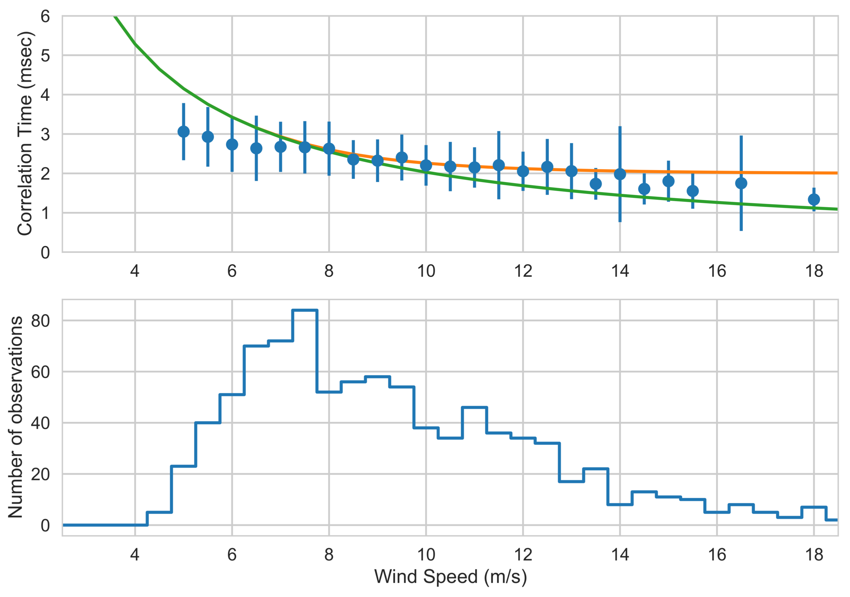
3.1. Ocean Temporal Correlation

The correlation time of the ocean backscatter cross section is the ultimate limitation on the accuracy that can be obtained from the Doppler method, since both signal-to-noise ratio or the Doppler bandwidth of the footprint can be reduced by transmitting more power or using a larger antenna. In the absence of temporal decorrelation, very long pulse separation could be used to improve radial velocity estimates. Given the importance of the surface temporal correlation time in determining and predicting the accuracy of the estimated radial velocity, it is important to note that the DopplerScatt spinning configuration can be used to estimate it directly. The Doppler bandwidth contribution vanishes in the fore and aft directions, so that the only contributions to the correlation are the constant noise correlation factor, ${\gamma }_N$, and the ocean temporal correlation (4). We fit the correlation time by calculating the average correlation in the forward direction by averaging over 25 km along-track. The logarithm of the resulting value is fit with a quadratic, from which the correlation time can be derived. Figure 16 presents the results for the estimated correlation time as a function of wind speed. The data used spanned all of the data collections and had 25 km mean winds ranging between about 4 m/s to about 18 m/s. The mean temporal correlation time decreases with wind speed and ranges from a little over 3 ms to about 1 ms. Equation (4) predicts that the correlation time should be inversely proportional to the radial orbital velocity of ocean waves inside the radar footprint. Given the fine range resolution and relatively coarse azimuth resolutions, we expect that the total variance will be maximized when the waves are perpendicular to the look direction and minimized when traveling in the range direction. In Figure 16, we use the wind-driven Pierson–Moskowitz spectrum to compute the predicted correlation for both wave direction cases. The predicted results agree well with the simple Pierson–Moskowitz estimate, although the correlation time is shorter than expected at low wind speeds, due to the fact that in the wave radial velocity in those situations probably contains non-wind-driven swell contributions, which cannot be neglected.

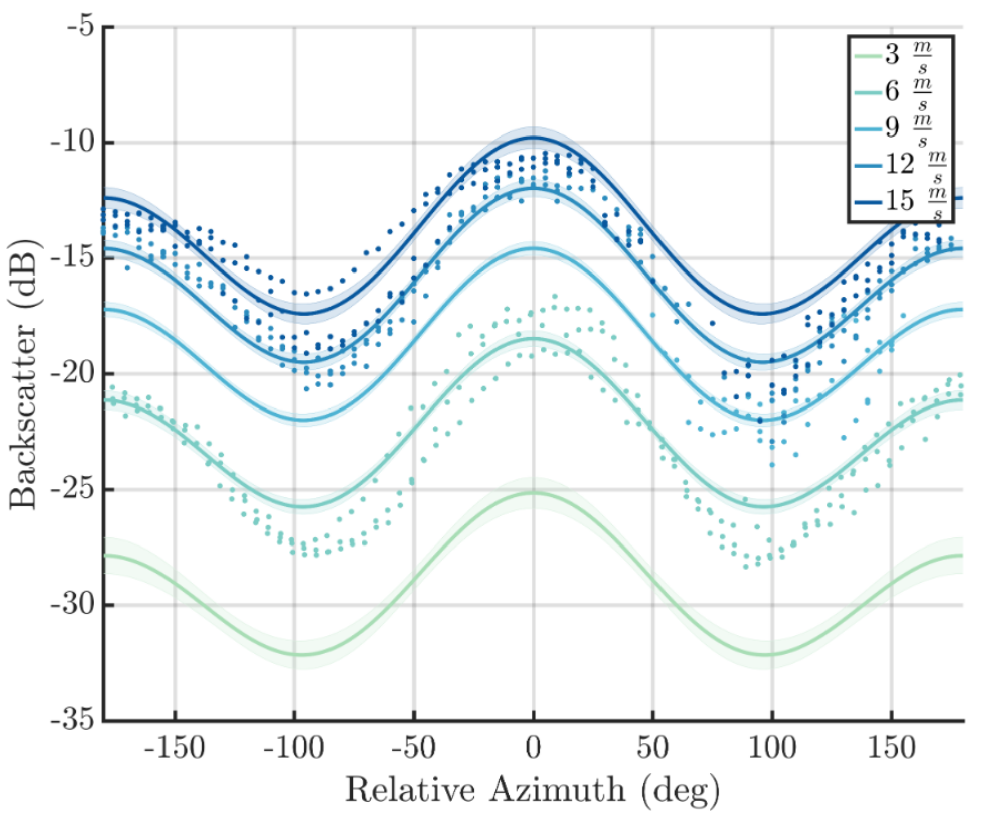
3.2. Wind Geophysical Model Function

With the launch of AltiKa in 2013 [36], a shift has begun towards higher frequency wind-observation instruments, but Ka-Band Geophysical Model Functions (GMFs) are rare. The majority of well validated scatterometer GMFs were developed using C or Ku-band data [37,38,39,40], owing to the large number of past scatterometers operating in those frequency bands. For years, a study by Masuko et al. using platform-measured backscatter from a Ka-band radar was the only available Ka-band GMF [41], although studies at near-nadir have shown a 6 dB offset from that model is necessary, likely due to calibration issues [42,43,44]. More recently, Yurovsky et al. [23] have derived a Ka-band wind GMF over a wide range of incidence angles using platform data called KaDPMod. This GMF more closely matches Ku-band GMFs and agrees fairly well with a 6 dB offset from Masuko. However, due to the nature of platform measurements, the data set used for training KaDPMod is sparse over azimuth, causing some potential uncertainties in the azimuth modulation.

We have developed a V-pol Ka-band GMF for incidence angles around ${56}^{°}$ using airborne data taken during the four DopplerScatt campaigns. Wind speeds and directions interpolated and collocated to DopplerScatt L1B data were taken from the highest resolution models available for each deployment. In the case of data taken near the Monterey Bay, the North American Mesoscale Forecast (NAM) (https://www.ncdc.noaa.gov/data-access/model-data/model-datasets/north-american-mesoscale-forecast-system-nam) model was used with a 3 km spatial resolution and time steps of 1 h. For data taken off the coast of Mississippi, a 250 m spatial resolution University of Miami Unified Wave INterface-Coupled Model (UWIN-CM) (https://www.gitbook.com/book/milancurcic/uwincm-manual/details) was used with time steps of 1 h. For data collected off the Oregon coast, we used the National Oceanic and Atmospheric Administration (NOAA) Blended Sea Winds (https://www.ncdc.noaa.gov/data-access/marineocean-data/blended-global/blended-sea-winds), which blend satellite observations and NCEP winds with a spatial resolution of ${0.25}^{°}$. In total, about 7.2 million data points were collected from incidence angles between ${53}^{°}$ and ${59}^{°}$ degrees, wind speeds between 3 m/s and 20 m/s, and all relative wind directions (thanks to DopplerScatt’s spinning antenna). The accuracy of each truth data at high resolution will vary with region and available data: e.g., high resolution SST might modify winds at high resolution and not be available in the forecast. The reader should refer to the links above for the expected accuracy of each model.

Prior to building a model function, data more than 3 dB from the peak of the antenna pattern was removed, as were data within 2 km of the coast (to avoid wind shadowing) or data flagged by quality control in the processing. Rain was not present in any of the data taken. Histograms of the training data set are shown in Figure 17, including the model winds used for training. Bins were populated with mean backscatter in a three-dimensional incidence, relative wind direction, and wind speed space. To remove outliers, an iterative binning approach was used during which backscatter measurements more than two standard deviations from the bin mean were removed. All binning was done in linear (non-dB) space. After binning, there were a total of about 18 thousand data points. Due to flight paths, coastlines tended to flag out data in the positive region of relative azimuth, resulting in the skewed distribution across relative azimuth. During the course of these data collections, we tended to fly over either high winds or low winds, with very few moderate wind speeds predicted by the models used.

Radar backscatter depends on the three variables considered here in different ways. With wind speed, backscatter follows a power law akin to $\log {\sigma }_0=A+B\log U_{10}$. This functional form matches the saturation typically experienced by scatterometers at high wind speeds. For DopplerScatt, we have found the value of B to be about 2. This predicts a saturation of somewhere around 20 m/s, consistent with other scatterometers [45]. A cosine expansion is typically used to represent the variation in backscatter over relative wind direction [46]

$${\sigma }_{°}=A_0(\theta ,U_{10})+A_1(\theta ,U_{10})\cos \left({\varphi }^{\prime }\right)+...+A_N(\theta ,U_{10})\cos \left(N{\varphi }^{\prime }\right),$$

(45)

where $A_0$ through $A_N$ are fitting parameters that depend on both incidence, ($\theta$), and wind speed, (U), and ${\varphi }^{\prime }$ is the relative wind direction (the azimuth angle between DopplerScatt’s look and the wind). Traditionally, the harmonic expansion is taken in real (not dB) space, but fitting in dB space offers some advantage for noisy data and, and will aid in comparison with Yurovsky et al. [23] who take this approach. We fit a harmonic series in dB space: the two fitting approaches are very similar if $A_n/A_0\ll 1$, but fitting in dB space may introduce higher harmonics in real space. Note that, due to tradition, for the wind GMF, we take ${\varphi }^{\prime }=0$ when looking in the upwind direction; i.e., in a direction opposite the wind direction. Following the oceanographic convention, we take the downwind direction as the reference (e.g., for the current GMF relative direction). The $A_N$ dependence on temperature is not considered here. Often, Equation (45) is fit separately for multiple incidence angles and wind speed regimes to break out the wind speed/incidence behavior; however, in order to fit a single model function over all wind speeds and incidence angles, an integrated model was used, similar to Yurovsky et al. [23]. This helps to interpolate the data set we are fitting over data-sparse parts of parameter space, but also introduces the possibility of incorrectly biasing the fit (e.g., only a single power law in speed is assumed for the entire speed range). We believe our data set has enough data to use an integrated model while still benefiting from this technique.

The functional form shown in Equation (46) was chosen to include a cosine expansion in relative azimuth, a logarithmic speed dependence, and a linear dependence on incidence angle. The form is the same as the Yurovsky et al. KaDPMod functional form, besides the linear incidence dependence, which was reduced from a fourth order to a first order polynomial because DopplerScatt only views a relatively small range of incidence:

$$10{\log }_{10}{\sigma }_0=\sum _{n=0}^2\sum _{m=0}^1\sum _{k=0}^1{C}_{nmk}\cos n{\varphi }^{\prime }{\theta }^m{\left({\log }_{10}{U}_{10}\right)}^k.$$

(46)

Equation (46) expands to a 12 coefficient model function, for which least squares optimization was done to determine the coefficients shown in Appendix C. The least squares fit results in a root mean square error of about 2 dB. Comparing actual to predicted backscatter in Figure 18 finds no significant bias or unaccounted model shape. Over the range of incidence angles measured, this model function appears to be a good fit, but we cannot recommend its use outside of the trained range of ${54}^{°}–{59}^{°}$ incidence.

Figure 19 shows the DopplerScatt GMF shape at ${56}^{°}$ incidence and various wind speeds and relative azimuths, along with the corresponding binned data used for fitting. The fit again appears to be a good representation of the underlying data. Beyond the goodness of fit, the GMF shape saturates as wind speed increases and modulates from highest return at upwind to low return at cross wind. Fit error is shaded behind wind speed curves and represents 95% confidence intervals.

The wind speed dependence of the azimuth-averaged GMF, the underlying binned data variability, and the Ku-band GMF for ${56}^{°}$ incidence from NSCAT/QuikSCAT are shown in Figure 20. Simulated backscatter data from the GMF and binned training data was averaged into wind speed bins for both 55 and 56 degrees incidence. The GMF follows observations and the theoretical power law well, with saturation somewhere above 15–20 m/s. This is consistent with Yurovsky et al., where they found saturation beginning at 15 m/s. Variations with incidence angle are small, as might be expected for 1 degree variation, but consistent across wind speed. Figure 21 considers the relative-azimuthal dependence of ${\sigma }_0$ over wind speed by separating between down-wind (${\varphi }^{\prime }={180}^{°}$), up-wind (${\varphi }^{\prime }=0^{°}$) and cross-wind (${\varphi }^{\prime }={90}^{°}$). Here, we again see the expected power law dependence of both the observations and the simulated GMF data. As we might expect, we see a consistent difference between the three wind direction regimes, with upwind consistently presenting the largest return signal, followed by downwind and finally cross-wind. While this plot seems to indicate some saturation at wind speeds above 15 m/s, we have not found that to be the case during wind retrieval compared to buoy measurements. We have found that the model wind estimates used to bin against were low relative to the actual winds, which could incorrectly lead to saturation. Compared to the previous plot, Figure 20, we see smaller error bars since we are no longer averaging over all relative azimuths. Unlike Figure 20, the fits for the azimuth cuts do not follow the data as well for the highest wind speeds, possibly pointing to limitations in the fitting model over the full set of azimuth angles. Additional high wind speed data is required to resolve this issue.

In Figure 22, we compare the azimuthal and wind speed variations of the DopplerScatt, NSCAT, and KaDPMod GMFs. The DopplerScatt GMF is similar to the KaDPMod GMF but with some important distinctions. The most obvious difference between the two GMFs is that there is significantly more modulation between upwind and downwind in the DopplerScatt GMF than in the KaDPMod GMF. We believe this difference stems from the data sets used for fitting. KaDPMod has a sparse data set across relative azimuth (by nature of platform measurements), while the DopplerScatt GMF benefits from relatively even sampling across relative azimuths. The sparsity of the KaDPMod training data set (particularly in our incidence range) could effectively lead to interpolation across relative azimuth and incidence when fitting, leading to a smoother objective function across relative azimuth. This is the danger when fitting an integrated model function, as we discussed earlier. Based on private communications with the KaDPMod team, we found that the platform data collected in the DopplerScatt incidence range corresponds well with the DopplerScatt GMF. Despite the differences between the two fit GMFs, the correspondence of the underlying data sets is a good indicator of calibration between the two experiments.

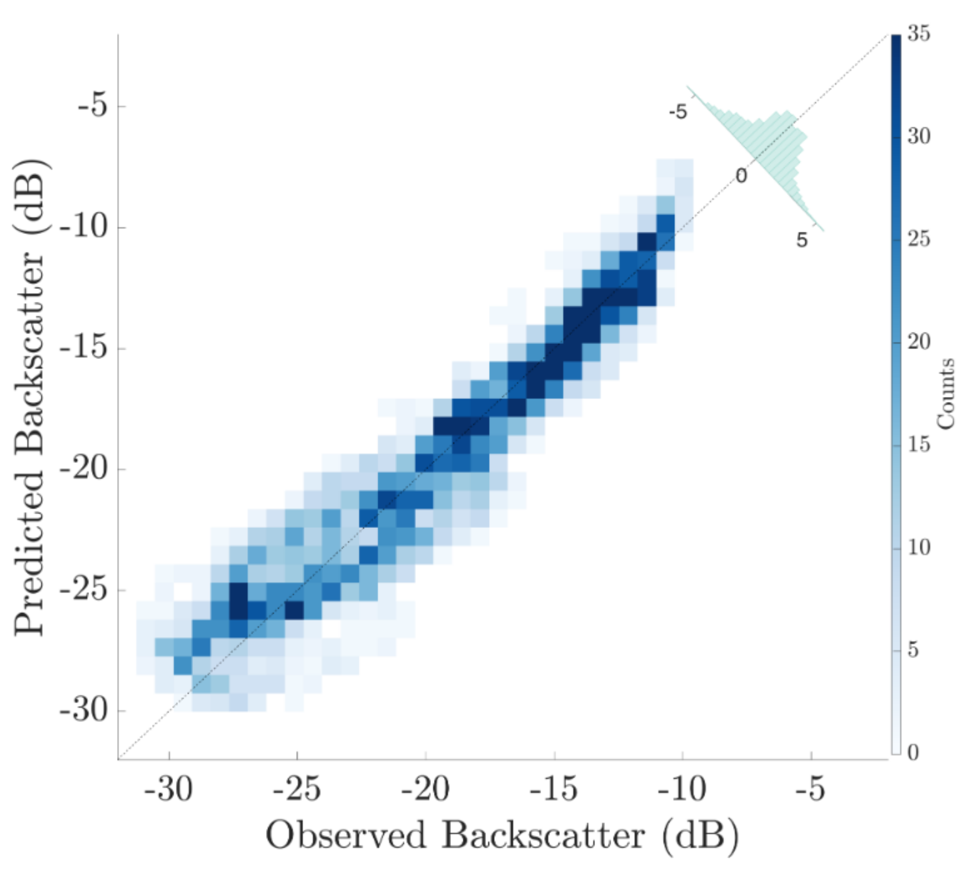
3.3. Wind Retrieval Results

Results from a particularly interesting DopplerScatt deployment off the coast of Louisiana during the SPLASH campaign are shown here. On 18 April 2017, DopplerScatt flew over the area containing the Mississippi River plume and Barataria Bay. Looking at DopplerScatt ${\sigma }_0$ data in Figure 23, there are distinctive features, potentially due to a combination of local flows and surface characteristics. Just right of the center in Figure 23, the Mississippi river plume is clearly visible as a low backscatter feature. The river outflow and coastal currents move towards the west (left) in the south, but curve north at the edge of Barataria Bay and recirculate to the east (right) near the coast (see models and results in Section 3.5). This effect is probably due to surface films or atmospheric boundary stratification, although water viscosity can also important role in determining how the wind forces capillary waves, especially at low temperatures. Additionally, scatterometers measure the wind speed relative to the moving surface current frame [1], so, since winds were mainly in the northwest direction (Figure 24), we can also expect the changes in direction in the current to show up as decreased backscatter when the current moves with the wind, while backscatter is expected to increase when the current moves against the wind. Both of these changes are observed, although changes due to cooler plume waters, or current divergence, could be responsible for some of the decrease in the plume region. This flight area also includes a large number of highly reflective oil platforms, one of which was leaking oil at the time. Near the leaking platform, at ${28.9}^{°}$ N latitude and ${89}^{°}$ W longitude, what is likely an oil trail is visible as low backscatter.

Figure 24 shows the retrieved vector winds as estimated by DopplerScatt on 18 April 2017. Stepping back from the features, DopplerScatt estimated winds blowing towards the northwest at about 6.5 m/s. Data from the UWIN-CM model and data from NOAA’s Real Time Mesoscale Analysis (RTMA) indicate winds blowing towards the northwest at about 6 m/s, but without any of the smaller features evident in the DopplerScatt data. Comparing the RTMA model to DopplerScatt results in a direction RMS of 25${}^{°}$ and a speed RMS of 2.7 m/s, quite good considering the strong features picked up by DopplerScatt but not the models.

As expected, retrieved winds from 18 April display prominent wind speed features in the areas where the Mississippi river flows through the bay. Currents and winds are generally aligned in the area where currents flow out of the Mississippi river and towards the left (west), resulting in a reduction in measured wind speed. The opposite is true where the river outflow currents wrap back around and flow against the wind. Based on data from the Advanced Very High Resolution Radiometer (AVHRR), there is about a 2 °C difference in temperature between the Mississippi river outflow and the surrounding ocean water. Studies have found a 0.25 m/s to 0.5 m/s decrease in wind speed when sea surface temperatures quickly drop by 1 °C [47]. We believe the combination of surface currents and temperature changes are both apparent in the nearly 3 m/s drop in wind speed across the Mississippi river outflow. It is likely that additional modulation due to surfactants, salinity and dissolved solids play a part in the river outflow, too, through viscosity effects.

Shifting now to the overall DopplerScatt winds dataset, Figure 25 compares collocated buoy wind measurements with DopplerScatt wind estimates. For our flights, we only found five buoys that were close enough to DopplerScatt swaths for use. Median DopplerScatt data was taken over a 1 km grid and plotted against hourly buoy data within 15 min and 200 m (one grid cell) from buoy measurements. In total, about 100 buoy measurements were available and close enough to DopplerScatt data for use. Stability effects were not considered when comparing buoy winds to DopplerScatt winds, since we did not have sufficient information to calculate neutral winds. Since DopplerScatt measures wind speeds relative to the moving ocean surface, we can also expect larger differences in wind speed between DopplerScatt and buoys in areas of strong surface currents. No correction was made for this effect.

DopplerScatt wind directions compare favorably with buoy measurements, with the majority of points lying close to the $y=x$ line. Overall RMS direction difference versus buoys is about ${18}^{°}$. DopplerScatt wind speeds also compare well with buoy wind speeds, with 1.5 m/s RMS difference. In addition, 18 and 20 April each observed strong surface currents in the Mississippi river plume that, in the area of buoy measurements, caused a decrease in DopplerScatt estimated wind speeds. This decrease is apparent in the buoy comparisons. Another comparison was made using two models collocated to the DopplerScatt swath: a high resolution UWIN-CM model run for the Gulf of Mexico, and the NOAA’s RTMA, an hourly 3 km scale global assimilation. Compared to the same buoys, the UWIN-CM model finds an RMS wind speed difference of 2.6 m/s and RMS wind direction difference of ${57}^{°}$. The RTMA model finds an RMS wind speed difference of 5.1 m/s and RMS wind direction difference of ${61}^{°}$. DopplerScatt winds offer a significant improvement over these two models in the areas studied, probably due to the proximity to the coast and the fact that the model was not able to assimilate high resolution SST measurements (M. Curcic, private communication).

Consider now the DopplerScatt winds estimated using a heavy weighting on uncorrected surface current directions, where we also find satisfactory comparisons with buoy data (see the bottom panes in Figure 25). This time, however, there appears to be a 10 degree bias between DopplerScatt wind directions and Buoy wind directions. Since the “wind directions” estimated in this version of the processor are essentially uncorrected surface current directions, which reflect the direction of wave propagation for wind driven waves, we can expect a positive bias between buoy winds and this version DopplerScatt winds based drift angles observed by High-Frequency (HF) radars [48], although the exact angle of the difference will depend on the upper layer current structure. The ${\sigma }_0$-based directions do not consistently find this direction bias relative to the collocated buoys.

3.4. Surface Current Geophysical Model Function

The DopplerScatt polarization and incidence angles were chosen to simplify the interpretation of measured Doppler as surface currents. By choosing a moderate to high incidence angle, ~${56}^{°}$, one minimizes the tilt modulation effects present at lower incidence angles, while also minimizing wave breaking contamination that is common at higher incidence angles [31,32]. Using vertical polarization further minimizes breaking wave contamination, since double-bounce scattering only dominates for horizontal polarization [31,32]. For the incidence angles and polarization chosen, it is well known that radar backscatter, and therefore, the associated Doppler velocities, will be dominated by resonant Bragg scattering from capillary waves of wavelength ~5.1 mm [29,30,31,32]. The exact resonant wavelength and reflection coefficient are modulated by the local large wave slope. Since the Bragg wavelength ~$1/\sin \left(\theta -\zeta \right)$, where $\zeta$ is the large-wave slope in the look direction, the range of Bragg wavelengths, assuming large-scale wave slopes $\pm {10}^{°}$, will only vary between ~4.6 mm to ~5.9 mm, so that the Bragg waves are always capillary waves. In the absence of currents or large-scale waves, these capillary waves (if not phase bound to other waves) will propagate with a nominal phase speed of 31 cm/s. which only varies between 32 cm/s and 29 cm/s for the range of large scale slopes considered before. If the Doppler velocities were due only to the Bragg waves modulated by surface current, ${\mathbf{v}}_S$, the surface-projected radial velocity would be of the form

$$v_{rS}(\phi ,{\phi }_U,\theta )=\frac{{\mathbf{v}}_S·\widehat{\ell }\left(\theta ,\phi \right)}{\sin \theta }+\left({\alpha }_{+}\left(\phi -{\phi }_W\right)-{\alpha }_{-}\left(\phi -{\phi }_W\right)\right)\frac{c_B\left(\theta \right)}{\sin \theta },$$

(47)

where ${\alpha }_{+}$(${\alpha }_{-}$) is the fraction of Bragg waves moving along(against) the direction defined by the look vector $\widehat{\ell }$, and $\phi$ and ${\phi }_W$ are the look vector and wind direction azimuth angles, respectively. Thus, the surface-projected Doppler velocity should have a surface current term that is proportional to the cosine of the angle between the look vector and the surface velocity, and a term that depends on the difference in azimuth angles between the look and wind directions. Using a small footprint, vertically polarized X-band data at high incidence angle, Moller et al. [49] observed this behavior, after subtracting an along-wind wind-drift surface velocity component equal to $3.5$% of the wind speed.

This simple relationship can break down for two reasons. First, there is significant evidence that a significant fraction of the Bragg waves can be bound to longer waves and will travel at the longer wave phase velocity [30,31,50]. In that case, the waves will be mostly concentrated on the leeward face of the larger wave, near the crest. It is expected that, in the field, bound waves might have a significant contribution at lower wind speeds, while higher wind speeds might exhibit a larger proportion of free waves. There is no clear data at this point to determine the exact proportion and contributions to the Doppler for different ocean surface conditions, although Plant and Irisov [31] have made a start for the backscatter cross section.

Another effect appears when the radar footprint is not small compared to the large-wave wavelength [8]. Because the large-scale waves modulate the amplitude of the Bragg waves (and, hence, ${\sigma }_0$) in a way that is correlated with the large wave phase, the large-wave radial velocity contribution to the Doppler will not cancel, since the Doppler measured at the radar is the ${\sigma }_0$-weighted average of the Doppler velocities over the waves (see Appendix A for details). Chapron and co-workers [8,13,19,20,21] have shown that, for C-band data at moderate incidence angles, there is a strong and quasi-linear dependence between the measured Doppler velocities and the wind speed. They attribute this to the effects of large-scale surface tilt and hydrodynamic modulation, which result in an effective amplification factor G to the wave Stokes drift (see Section 4 for additional details).

Without wanting to prejudge the mechanisms operating at Ka-band, we assume that the measured Doppler surface velocity is given by

$$v_{rS}=\frac{{\mathbf{v}}_{SE}·\widehat{\ell }\left(\theta ,\phi \right)}{\sin \theta }+F_S\left(U_{10},\phi -{\phi }_U\right),$$

(48)

where ${\mathbf{v}}_{SE}$ is the Eulerian part of the surface current that is not responsive to the local wind, and $F_S$ represents the contribution of the local wind to the surface current. The wind contribution to the current will not only be composed of the wave modulation effects discussed above, but will include surface currents due to Stokes drift, surface drift Lagrangian (~0.01–$0.03U_{10}$) and Eulerian ($\sim 0.01U_{10}$) components [48,51,52,53]. This wind-driven surface current sensed by the radar will represent the depth averaged current over a fraction of the Bragg wavelength [54], which will be on the order of a millimeter. Given the large shears expected very near the surface [50], it is not clear that the earlier estimates used for HF or C-band radars will apply, and, considering also the presence of bound waves, we do not assume a linear (or near-linear) model for the dependence on wind speed. Similarly, the Stokes drift, Lagrangian, and Eulerian wind driven components are known to have different directions relative to the wind direction. In what follows, we only assume that the net effect of all these contributions will have a systematic dependence on the the wind direction (which might vary with speed), but do not assume that the peak of the response will be along the wind direction.

To estimate $F_S$, we only assume that, over our data set, ${\mathbf{v}}_{SE}$ is independent of the current components driven by the local wind, which given the variety of wind conditions and locations that we sampled in our data collections, is a reasonable assumption. To make a non-parametric estimate of $F_S$, we bin our data with respect to the local wind speed and relative wind azimuth direction observed by DopplerScatt. To explore the directional dependence of $F_S$, we used both the wind direction derived with slight nudging from the total Doppler current direction, and the direction heavily weighted by the total Doppler current direction, which reflects the net direction of wind and local currents. The results of this binning process are shown in Figure 26 for directions weighted heavily by the total Doppler direction, which have about a ${10}^{°}$ offset to the right relative to the buoy wind direction, cf. Figure 25d. To estimate the variability around the mean for each histogram, we assumed that data sets collected on different days were independent (consistent with our wind variability) and used the jackknife resampling method [55] to estimate the standard deviations (shown in grey shading) corresponding to the mean values (shown as dashed red line). The result for lightly nudged directions (not shown), which are unbiased relative to buoy directions, is very similar, but shows greater variability, especially at higher winds.

Examination of the results of binning with the two wind directions shows very similar behavior with respect to the wind speed dependence. For very low wind speeds (upper-left panel), where few long-wavelength waves are assumed to be present, the surface scatterers propagate at (or near) the phase velocity of the free Bragg-resonant capillary waves (~31 cm/s), and the shape of the flat-topped wide response is similar to that observed by Moller et al. [49]. However, as the wind speed increases to about 4.5 m/s, the peak velocity increases and the shape of the distribution begins to approximate a sinusoid. For wind speeds greater than 4.5 m/s, the peak of the distribution remains approximately constant, up to higher wind speeds (~13 m/s), where a slight increase seems to occur, although there is significant scatter around the mean, making this trend less certain. Even though the shape is roughly sinusoidal, some bias and kurtosis are apparent. Examining the variability around the mean, it is also clear that the scatter around the mean is significantly less when the total Doppler directions are used, indicating that the direction of the wind-driven Doppler currents are not along the wind direction, but offset to the right, as expected for a mixture of Lagrangian and Eulerian wind drift currents. However, the magnitude of the current is significantly higher than that expected for the wind drift currents.

To get a more quantitative assessment, we fit the histograms with the 4th-order harmonic expansion given in Equation (33). The results for both wind directions are presented in Figure 27 and tabulated in Appendix D. It is clear from this figure that the dominant behavior of $F_S$ is given by the first harmonic (i.e., pure velocity vector), which increases linearly from the free wave Bragg velocity to about 75 cm/s at a wind speed of 4.5 m/s, and remains approximately constant thereafter, with a small increase at higher wind speeds. It is also clear from this figure that the parameters derived by binning with the wind direction (green) are significantly noisier than those that use the total Doppler direction (blue) (Recall from Section 2.6 that, for wind speeds less than about 6 m/s, the directions are mostly determined by the total Doppler direction.). The term $\delta {\phi }_U$ (lower right panel) shows the systematic difference in direction relative to the wind direction observed in the buoy comparisons, for the wind directions not heavily weighted by the total Doppler current direction.

The $\delta v_r$ and $v_{r2}$ parameters will introduce an upwind-downwind difference in $F_S$ and we plot the magnitude of this difference in Figure 28, which is small for low winds, but increases to about 10 cm/s for medium winds, while decreasing for higher winds. Since there is no reason for the true wind driven currents to be different in the upwind and downwind directions, we ascribe this difference to the effect of large-scale wave modulation of the scatterers. The third and fourth order harmonics are generally small, and not nearly as significant as the other parameters. Additional discussion of the behavior of $F_S$ and its relation with observations at other bands will be presented in Section 4.

3.5. Ocean Current Retrieval Results

The comparison of synoptic surface current fields against in situ data is not easy since the radar measured surface velocity is effectively at the surface, but in situ instrumentation typically measures the current at some depth. HF radars measure at a depth dependent on the radar wavelength [48,54], which can be on the order of a meter, while surface drifters will measure currents at the depth they were drogued. For our flights, we only had limited HF radar coverage and, although a large number of drifters were deployed for SPLASH, they quickly converged along fronts and did not provide a synoptic measurement of the total area covered by DopplerScatt. The detailed comparison of DopplerScatt currents against these data is beyond the scope of this paper and will be addressed in a subsequent publication.

To assess how reasonable the DopplerScatt synoptic measurements were, we will compare our current retrievals against forecasts from the Navy Coastal Ocean Model (NCOM) [56] ocean model running within the Coupled Ocean/Atmosphere Mesoscale Prediction Systems (COAMPS) system produced by the NRL Ocean Dynamics and Prediction group, which were provided to us courtesy of Dr. G. Jacobs (NRL) and the CARTHE/SPLASH team. Though the COAMPS system contains ocean, wave, and atmospheric models, only the ocean model was run with external atmospheric forcing as input. For the forecasts available to us, the main outflow of the Mississippi was routed to a different mouth than the one the river actually used, so that the representation of the Mississippi plume was not realistic (G. Jacobs, private communication), but the model, which was run at 250 m resolution, gave a fair representation of the general submesoscale features in the area.

Figure 29 presents the comparison of the DopplerScatt retrieved current components against their NCOM equivalents for data collected on 18 April 2017, as in the wind retrievals shown previously. The DopplerScatt data have been masked along the nadir track and the outer swaths where the estimated errors were greater than 20 cm/s (cf., Figure 10), leading to gaps in the coverage, which are greater for the V (north) current component than for the U (east) component. As can be seen from this figure, DopplerScatt captured well the general clockwise recirculation of the Mississippi plume and westward current into Barataria Bay. Both the model and the DopplerScatt measurements show a strong submesoscale front developing in the north-east quadrant of the Bay, but the exact location of the front is a bit further west in the NCOM data. An additional source of comparison that is helpful in the location of the plume, circulation, and the submesoscale front are provided by optical data obtained by the Sentinel-3 satellite (Courtesy of Copernicus Sentinel, processed by ESA), which is compared against the DopplerScatt surface current U-component in Figure 30. The figure shows close agreement with DopplerScatt in the location of both the river plume and the submesoscale front.

Although not definitive, we conclude that DopplerScatt data seems to have a good overall agreement with NCOM and optical data, given model forecast limitations, both in the features present and in the magnitudes of the currents. A more detailed comparison with both NCOM and in situ measurements will be presented elsewhere.

4. Discussion

Our results in the previous sections show that, although initially the effective wind-driven surface currents vary linearly with wind speed, the dependence decreases substantially for wind speeds ~4.5 m/s and greater. This is in contrast with the C-band results [8,13], which exhibit a strong dependence on wind speed for most of the observed wind speed range. In Appendix E, we present the theory behind the wind-driven surface current component, and show that it can be written as the sum of free (Equation (A58)) and bound (Equation (A60)) Bragg waves propagating along or opposite the azimuth look direction, and a term due to the uneven weighting of the large-scale wave orbital motion due to fluctuations of the Bragg spectrum:

$$\delta v_{rS}=〈\frac{\delta {\sigma }_0}{{\sigma }_0}\frac{\widehat{\ell }·\delta {\mathbf{v}}_W}{\sin \theta }〉=\cos {\varphi }_r\left(-\frac{\partial \log {\sigma }_0}{\partial \theta }\cot \theta U_S+〈u\frac{\delta B}{B}〉\right)-\cot \theta 〈w\frac{\delta B}{B}〉,$$

(49)

where $\delta B/B$ are the normalized fluctuations of the Bragg wave (saturation) spectrum; $U_S$ (Equation (A65)) is the deep-water Stokes drift current; ${\varphi }_r$ is the look direction azimuth angle measured relative to the down-wind direction; and u and w are the horizontal and vertical orbital velocities, respectively. There are several mechanisms for local Bragg spectrum variations, including modulation of small waves by winds and larger wave orbital velocities [57]; enhanced roughness due to wave breaking [58]; or generation of Bragg waves due to wave straining [31]. Rather than select among these mechanisms, several of which will likely apply at any given time and that are still not fully understood theoretically, we assume that, to the lowest order, the spectral modulation can be captured as a linear effect through a Modulation Transfer Function (MTF) [59], as defined in Equation (A66). In that case, we obtain a simple equation for $\delta v_{rS}$

$$\delta v_{rS}=U_S\left[\cos {\varphi }_r\left(-\frac{\partial \log {\sigma }_0}{\partial \theta }\cot \theta +\overline{m_r}\right)-\cot \theta \overline{m_i}\right],$$

(50)

where $\overline{m_r}$ and $\overline{m_i}$ are the averages of the MTF real and imaginary parts, weighted by the Stokes drift for each wavenumber (see Equation (A68)). This equation is equivalent to that derived by [18,60] when the modulation transfer function is frequency independent. This result shows that the orbital velocity bias is proportional to the Stokes drift current, and consists of two terms: the first term, proportional to $\cos {\varphi }_r$, behaves as a horizontal current and is due to coupling of the u-component of the orbital velocity and spectral modulations, as well as brightness modulation due to changes in radar brightness due to the large-scale wave slope. This first term changes sign when the look direction changes from downwind to upwind. The second term, due to coupling of the vertical component of the orbital velocity with spectral modulation, is independent of azimuth direction, and is responsible for the difference in upwind and downwind speeds that is shown in Figure 28. Using the results shown in this figure, we can estimate the imaginary part of the modulation function as

$$\overline{m_i}=\tan \theta \frac{\delta v_{rS}({\varphi }_r=\pi )-\delta v_{rS}({\varphi }_r=0)}{U_S}.$$

(51)

To obtain an estimate as a function of wind speed, we assume that the Stokes drift can be linearly related to wind speed, $U_S=\beta U_{10}$. To compare against other experimental data, we take $\beta =0.01$, which lies in the mid-range of values given in [48] (although $\beta$ might itself contain some wind speed variation), and present the results in Figure 31. We note in this figure the change of sign in $m_i$, which implies $〈w\delta B〉<0$, which implies that, at high wind speeds, capillary wave roughness is enhanced in the windward, rather than leeward, wave crest. This is consistent with past Ka-band observations and with the hypothesis proposed by Yurovsky et al. [58] that this enhanced roughness may be due to the residual roughness due to wave breaking, which travels at a velocity slower than the larger breaking wave.

Once we have solved for $\overline{m_i}$, it is possible to model the $F_S$ data (Figure 26) as

$$F_S\left({\varphi }_r\right)=\overline{c_{pF}}\left({\varphi }_r\right)+U_S\cos {\varphi }_r\left[\left(\overline{m_r}+\frac{U_D}{2U_S}\right)-\cot \theta \frac{\partial \log {\sigma }_0}{\partial \theta }\right]-U_S\cot \theta \overline{m_i},$$

(52)

where we have ignored the Bragg bound wave contribution, assuming that under most open ocean conditions at moderate winds and above free waves dominate; $\overline{c_{pF}}$ (Equation (A58)) is the free Bragg wave contribution, such that $\overline{c_{pF}}\left(0\right)=-\overline{c_{pF}}\left(\pi \right)\approx 0.31$ m/s; finally, $U_D/2$ is the total wind drift speed at a given horizontal position averaged over wave motion, which introduces the factor of $1/2$ [61]. Due to the limited angular extent of our data collection, calculating $\partial \log {\sigma }_0/\partial \theta$ from the data itself, but we can estimate it from the theoretical Bragg cross section (Equation (A56)), the Ku-band NSCAT GMF, or the results from Yurovsky et al. [23], which all give similar results and we use the NSCAT result as the one with the greatest empirical data at high winds. Without a priori knowledge of $U_D$, we can only solve for an effective real part of the MTF, $\widetilde{m_r}\equiv \left(\overline{m_r}+U_D/2U_S\right)$, which includes not only wave modulation for total surface drift as well. Given these assumptions, we solve for $\widetilde{m_r}$ using the upwind and downwind data shown in Figure 28, and present the average of the upwind and downwind results in Figure 31.

We compare these results against Ka-band results reported by by Keller et al. [62] in the SAXON-FPN experiment in the North Sea; by Yurovsky et al. [58], acquired using a tower mounted radar in the Black Sea; and by Laxague et al. [63] using an optical set up that allowed for the resolution of Bragg-resonant waves in the high-frequency regime corresponding to Ka-band. Yurovsky et al. reported the MTF values averaged over frequency and fit with single power-law fit with respect to wind speed, which we present as the blue line in the figure. Keller et al. ([62], Figure 4) present the mean and variance of the Ka-band MTF averaged over the frequency range 0.25 to 0.3125 Hz, and we have fit a smooth polynomial through the means, which, after subtracting the tilt MTF appropriate for their ${45}^{°}$ incidence angle, we show as the green line in the figure. Laxague et al. subdivide the spectral variability obtained by optical means into a region appropriate for Ka-band, and derive an MTF, at a number of wind speed points, which we digitized and fit with a power-law, as with the other MTFs, and the results are shown in orange. The agreement between the estimated MTF and the one in the literature is fairly close for wind speeds above 6 m/s. The largest disagreement is with the results of [58] for $m_r$, but this may be partly an artifact of their modeling of $m_r$ as a simple power-law in $U_{10}$, since when we model our data in the same way, we also get large disagreements at lower wind speeds, as shown in Figure 31. At speeds below 4 m/s, the agreement is not as good between any of the models, perhaps reflecting the lack of data or the influence of non-wind-driven swell in the generation of brightness modulations. Note that improved agreement with the other models could be obtained by varying $\beta$ and/or making it wind dependent. Given the scatter between the different measurements, probably due to real-world variability, this is not a necessary refinement.

The main point of this discussion is to show that the wind speed behavior of $F_S$ is consistent with biases due to ${\sigma }_0$ variations along the large-scale wave via a linear modulation mechanism, and that the magnitude of this modulation is consistent with previous Ka-band results. To get a better understanding of the operating mechanisms, we present in Figure 32 the decomposition of the upwind and downwind wind-driven surface velocities into contributions due to free Bragg waves and tilt modulation, ${\sigma }_0$ coupling to u through $m_r$, and ${\sigma }_0$ coupling to w through $m_i$. We see that the free Bragg wave contribution accounts for the behavior at low winds, and the addition of tilt modulation, which is proportional to the Stokes drift, accounts for a slow increase with wind speed in the upwind and downwind biases. The rapid increase in $F_S$ at wind speeds smaller than about 4 m/s can be attributed to the rapid increase in the coupling to the u component through $m_r$. We speculate that this rapid increase may be due to the presence of bound waves in the leeward side of the wave crests that may be more noticeable at low wind speeds due to the smaller fraction of the area covered by free Bragg-wave patches. The relative stability between 4 m/s and 12 m/s is attributed to the fact that, in this range, $m_r$ decays with wind speed faster than $U_S^{-1}$ and this decay is sufficient to compensate the linear increase due to tilt modulation. Coupling to the vertical velocity component has a relatively small effect in the magnitude of upwind and downwind components, but is responsible for the asymmetry in the response, since the other mechanisms have the same magnitude and opposite sign, while the sign of $m_i$ does not depend on the look direction. We note that for wind speeds greater than about 12 m/s, the data scatter increases, but there is a small increase in the velocity magnitude, that could be attributed to $m_r$ decreasing more slowly at higher winds, potentially due to the effects of wave breaking. The bulk of the difference in the behavior of $F_S$ at Ka and C-bands [8,13] can be attributed to the fact that the C-band data was acquired at lower incidence angles, so that the tilt modulation factor $\partial \ln {\sigma }_0/\partial \theta$, which is ~3 at our incidence angles, can be as much as ~15 for the lower incidence angles of the C-band SAR data. However, we note that the empirically observed fast decay of $m_r$ with wind speed plays an additional role, as using the theoretical value [20] for $m_r$ results in greater wind speed dependence than we observe (F. Nouguier, B. Chapron, personal communication).

In the previous discussion, we dealt only with modulation effects due to waves traveling along the wind direction. To see how this one-dimensional assumption fits the data, we subtract the MTF modeled wind driven surface velocities from the observed velocities, and present the results in Figure 33. If the one-dimensional wave modulation accounted for all of the effects, the difference between these two lines should be $\overline{c_{pF}}$, which, according to Equation (A58), should vary in the range $\pm 0.31$ m/s with a top that reflects the broad capillary wave spectrum, as has been observed experimentally for narrow beam radars as reported by, e.g., Moller et al. [49]. This is indeed what is observed in Figure 33, where the $\overline{c_{pF}}$ results are quite similar to the ones obtained in [49]. The main discrepancy we observe is the fact that the zero-crossing of this function does not occur exactly at ${\varphi }_r=\pm \pi /2$, but is slightly broader in the downwind direction than upwind. We speculate that this difference is due to the fact that, due to the angular spreading of the large-scale wave spectrum, there will be a resulting asymmetry in the up and downwind directions. Nevertheless, we find that the simple MTF model provides a reasonable explanation of the $F_S$ features observed in the DopplerScatt data, although we selected to use the empirical version of $F_S$ when removing the wind-driven currents to account for the small disparities with the MTF model.

5. Conclusions

This paper has presented DopplerScatt, a new instrument that provides estimated simultaneous measurements of winds and currents using a Ka-band pencil-beam scanning Doppler scatterometer. With the development of DopplerScatt, we have extended the theory and calibration of these instruments beyond the existing literature [9]. Among the innovations presented in the system understanding, algorithms, and calibration, we note:

• Development of an end-to-end measurement model including several effects, such as quantifying the impact of cross-section variations, not previously reported.
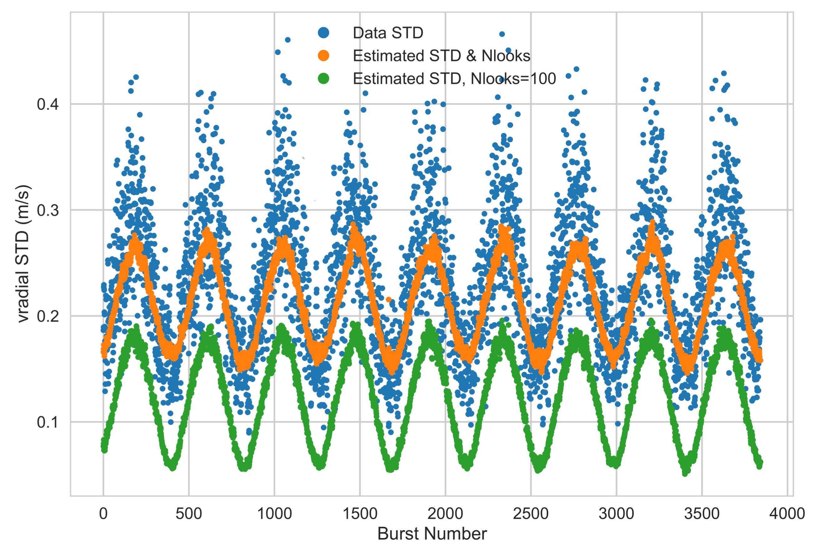
• Detailed examination of the pulse-pair estimation algorithm, including deriving an error estimator for the Doppler velocity and validating it with experimental data.
• Development of an end-to-end error budget including both random and systematic errors. The error model was validated against measurements and showed that the DopplerScatt instrument had good stability and noise performance for both ${\sigma }_0$ and Doppler velocities.
• Development of new calibration techniques to remove errors caused by uncertainties in the antenna pointing and other systematic (e.g., model function) errors.
• Development of a wind estimation algorithm that uses backscatter and Doppler velocities in an innovative way so that winds vectors can be estimated using a single beam, rather than the traditional two-beam architecture.

In addition to these technical innovations, we have collected an extensive data set of Ka-band V-pol ${\sigma }_0$ and Doppler velocities. Using these data, we have:

• Determined the ocean correlation time at Ka-band as a function of wind speed. The correlation times observed (>2 ms) indicate that this measurement is scalable to spaceborne applications with reasonable performance.
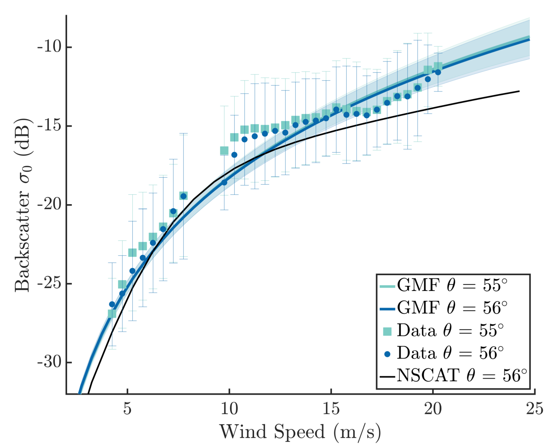
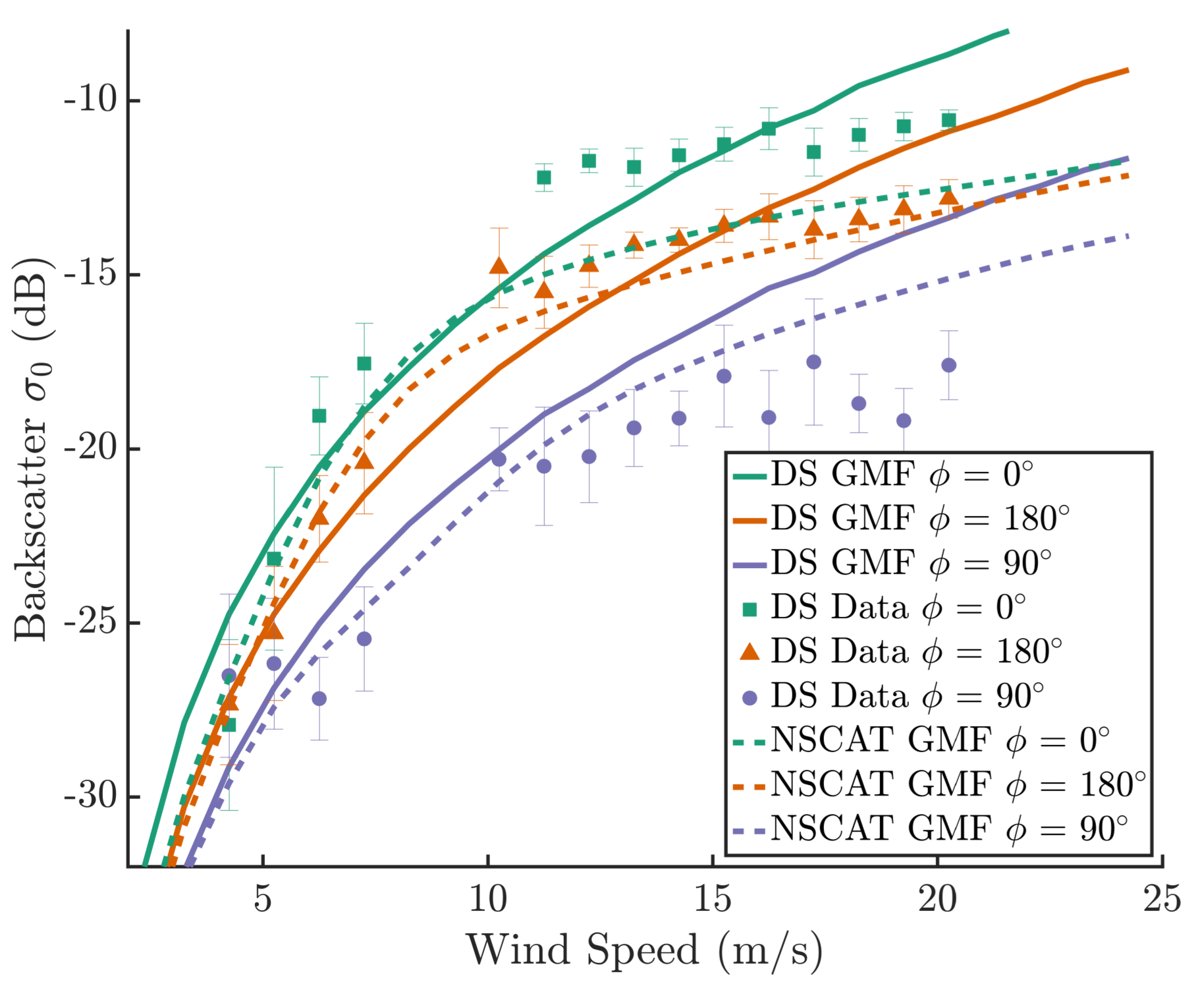
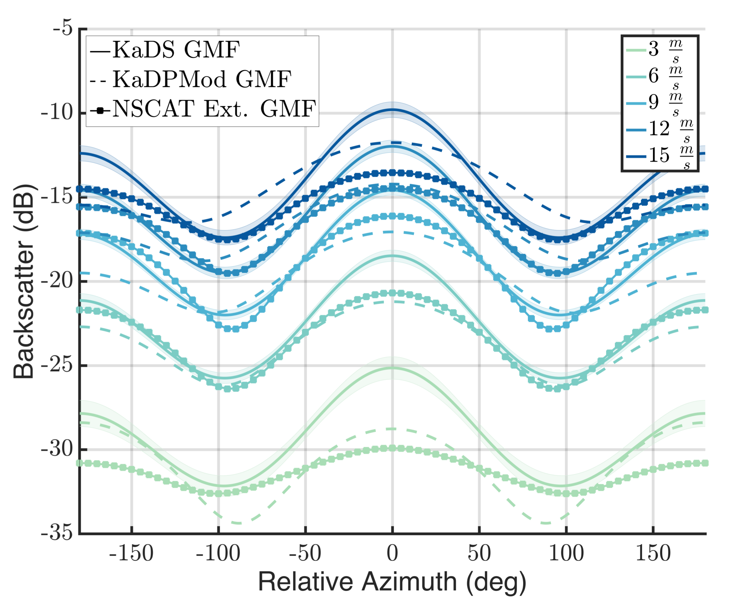
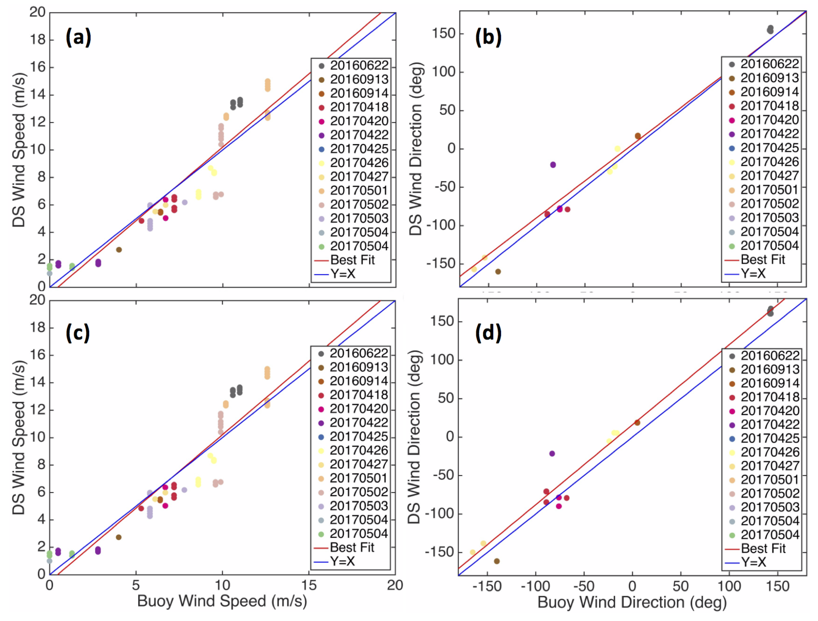
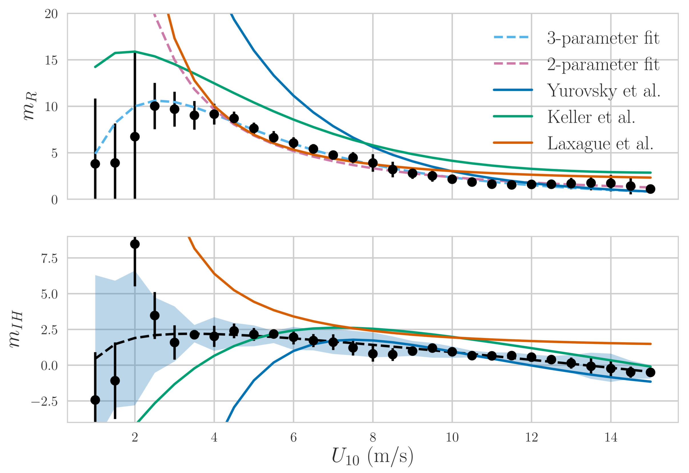
• Developed a Ka-band V-pol GMF which shows an overall sensitivity to wind speed similar to the one predicted by the Ku-band NSCAT GMF. The main difference between the two GMFs is in the much greater upwind cross-wind modulation seen at Ka-band, which will improve wind direction estimation. The observed modulation also exceeds the one observed at Ka-band from a platform in the Black Sea by Yurovsky et al. [23], but, due to platform geometry, the cross-wind sampling may not have been optimal for these incidence angles. Yurovsky et al. also have a global analytic form for their GMF that may constrain the modulation somewhat, and comparisons against actual data points (Yurovsky, personal communication) show better agreement with DopplerScatt observations than the analytic formula. Resolving these discrepancies will require additional data, but the current results, as well as those of Yurovsky et al., show that there is sufficient wind speed and direction sensitivity at Ka-band to obtain wind estimation performance similar to that of Ku-band scatterometers, such as QuikSCAT. Formal errors in the estimated wind speed and direction indicate performance better than spaceborne scatterometers, but the limited comparison against buoy data shows similar performance, possibly pointing to needed improvements in the GMF, possibly including current effects.
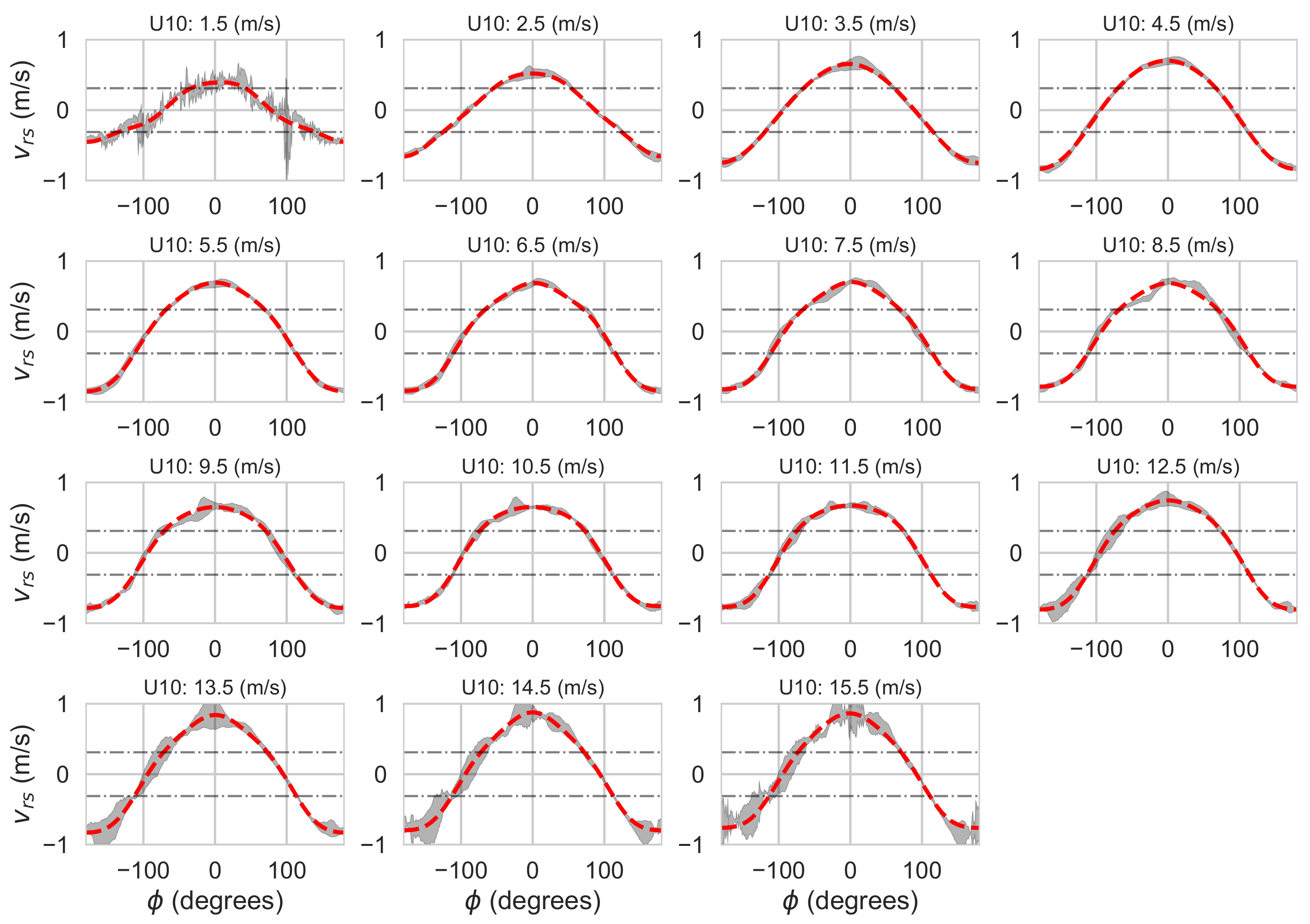
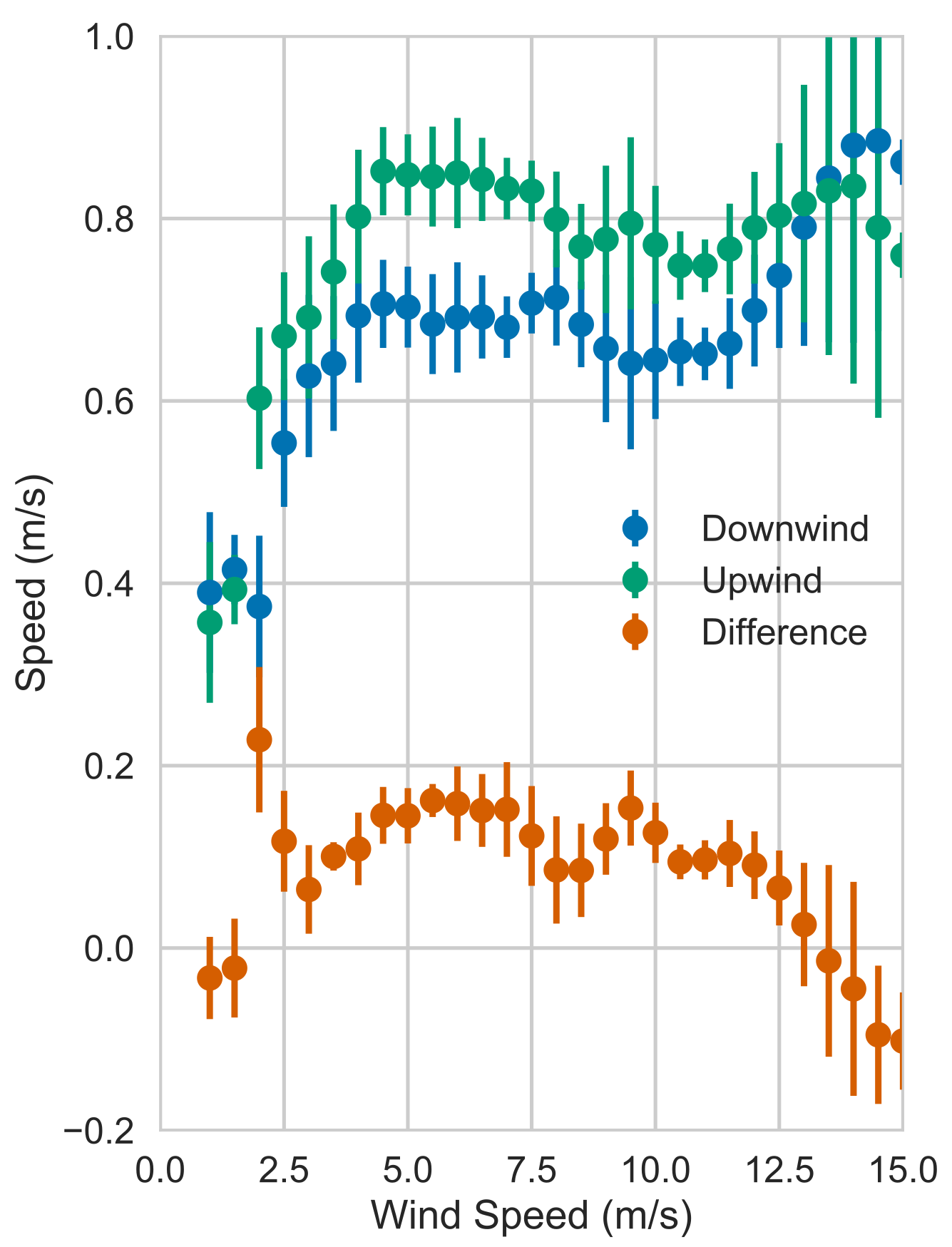
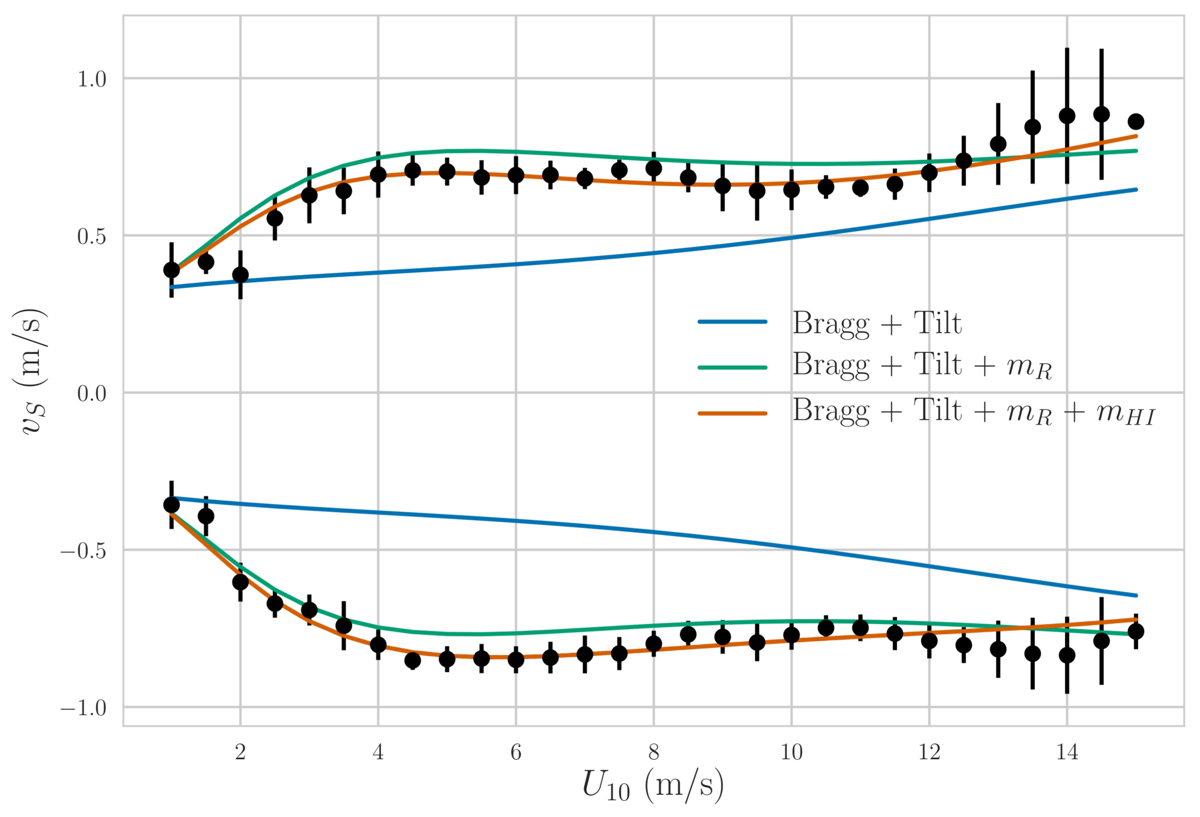
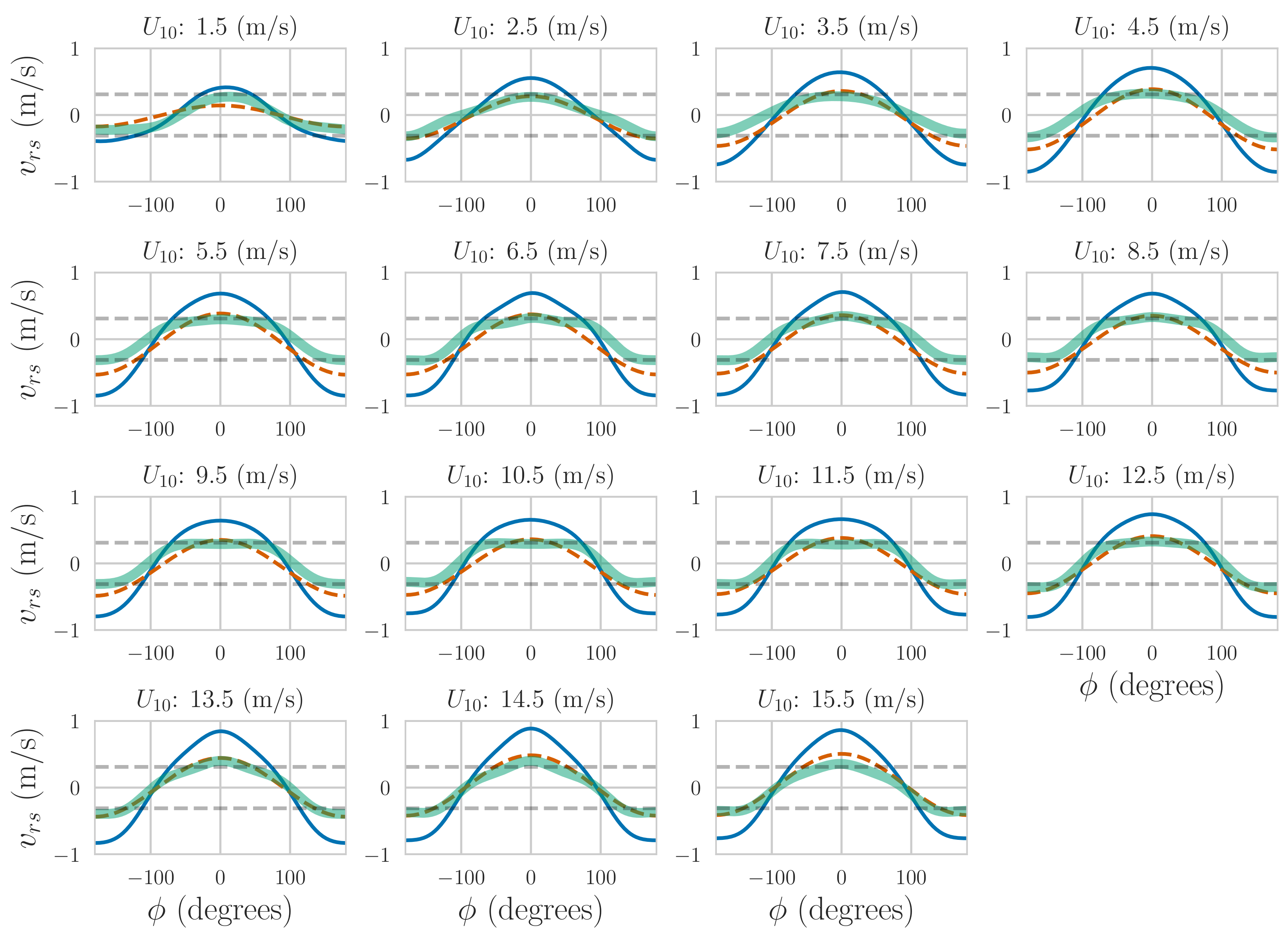
• Examined the local wind dependent part of the Doppler velocity signature. While the signature is roughly aligned with the wind direction, as for other frequencies, it deviates slightly from the true wind direction, in a fashion consistent with expected direction differences consistent with those expected for the sum of Lagrangian and Eulerian wind-driven currents [48]. However, the wind speed dependence of the Doppler currents is quite different from the one observed at C-band [8,13], where the Doppler velocity is nearly linearly dependent on wind speed. By contrast, at Ka-band, there is only a linear dependence for low winds, and the magnitude of the dependence stabilizes after a wind speed of about 4.5 m/s. In addition, the shape of the wind-dependent response is close to a sinusoid with azimuth angle; i.e., the expected response of a constant velocity vector, albeit, one that seems to propagate at a small angle to the wind direction, consistent with wind-drift measurements with HF radars [48]. This behavior was explained as due to the modulation of the backscatter cross section through a modulation transfer function (MTF) consistent with those previously observed at Ka-band. The lack of dependence of the wind correction with respect to wind speed makes the estimation of the non-wind driven part of the surface current much less sensitive to wind speed variations, although still sensitive to wind direction errors. Given that the wind-dependent correction can be made with the same instrument used for estimating the Doppler velocities, this combination is scalable to a spaceborne instrument.

The contribution of the wind-driven ${\sigma }_0$ modulation to the estimated surface currents is on the order of $\pm 0.3$ m/s (see Figure 33), which is of the same order of magnitude as many surface currents and must be removed, in addition to the Bragg wave contribution. We rely on an empirical GMF for removing this wind-driven component to obtain estimates of the surface current. Like the similar wind GMF in scatterometry, the current GMF will need to be refined as additional data become available.

We note that the wind correction to the surface currents has scales characteristic of wind spatial scales, which are much longer than ocean scales. Therefore, residual errors in the surface currents due to errors in removing the wind-driven Doppler contribution will manifest themselves as approximate biases over submesoscale and small mesoscale local ocean features. This means that estimates of the surface current derivatives, which contribute to relative vorticity and divergence, key drivers of ocean transport, will be far less affected by errors in the GMF removal. The situation is also helped by the relative insensitivity of the current GMF over much of the windspeed range, which make GMF removal a more robust process than for other incidence angles or frequencies.

In the discussion above, we have assumed that waves were dominated by wind-driven waves, so that a relationship between wind and waves could be used. At low wind speed, swell, which is not generated locally by the wind, may play a role that needs further study. We have recently modified DopplerScatt to measure wave spectra, and will present results of this new mode in subsequent publications.

References

1. Kelly, K.; Dickinson, S.; McPhaden, M.; Johnson, G. Ocean Currents Evident in Satellite Wind. Geophys. Res. Lett. 2001, 28, 2469–2472. [Google Scholar] [CrossRef]
2. Small, R.J.; deSzoeke, S.P.; Xie, S.P.; O’Neill, L.; Seo, H.; Song, Q.; Cornillon, P.; Spall, M.; Minobe, S. Air-sea interaction over ocean fronts and eddies. Dyn. Atmos. Oceans 2008, 45, 274–319. [Google Scholar] [CrossRef]
3. Chelton, D.; Schlax, M.; Samelson, R. Summertime Coupling Between Sea Surface Temperature and Wind Stress in the California Current System. J. Phys. Oceanogr. 2006, 37, 495–517. [Google Scholar] [CrossRef]
4. D’Asaro, E.; Lee, C.; Rainville, L.; Harcourt, R.; Thomas, L. Enhanced turbulence and energy dissipation at ocean fronts. Science 2011, 332, 318–322. [Google Scholar] [CrossRef] [PubMed]
5. Goldstein, R.; Zebker, H. Interferometric radar measurement of ocean surface currents. Nature 1987, 328, 707–709. [Google Scholar] [CrossRef]
6. Goldstein, R.; Barnett, T.; Zebker, H. Remote sensing of ocean currents. Science 1989, 246, 1282–1285. [Google Scholar] [CrossRef] [PubMed]
7. Frasier, S.; Camps, A. Dual-beam interferometry for ocean surface current vector mapping. IEEE Trans. Geosci. Remote Sens. 2001, 39, 401–414. [Google Scholar] [CrossRef]
8. Chapron, B.; Collard, F.; Ardhuin, F. Direct measurements of ocean surface velocity from space: Interpretation and validation. J. Geophys. Res. 2005, 110, C07008. [Google Scholar] [CrossRef]
9. Bao, Q.; Dong, X.; Zhu, D.; Lang, S.; Xu, X. The Feasibility of Ocean Surface Current Measurement Using Pencil-Beam Rotating Scatterometer. IEEE J. Sel. Top. Appl. Earth Obs. Remote Sens. 2015, 8, 3441–3451. [Google Scholar] [CrossRef]
10. Fois, F.; Hoogeboom, P.; Le Chevalier, F.; Stoffelen, A.; Mouche, A. DopSCAT: A mission concept for simultaneous measurements of marine winds and surface currents. J. Geophys. Res. Oceans 2015, 120, 7857–7879. [Google Scholar] [CrossRef]
11. Freeman, A. On ambiguities in SAR design. In Proceedings of the EUSAR 2006: 6th European Conference on Synthetic Aperture Radar, Dresden, Germany, 16–18 May 2006; Jet Propulsion Laboratory: Pasadena, CA, USA; National Aeronautics and Space Administration: Dresden, Germany, 2006. [Google Scholar]
12. Madsen, S. Estimating the Doppler centroid of SAR data. IEEE Trans. Aerosp. Electron. Syst. 1989, 25, 134–140. [Google Scholar] [CrossRef] [Green Version]
13. Mouche, A.A.; Collard, F.; Chapron, B.; Dagestad, K.; Guitton, G.; Johannessen, J.A.; Kerbaol, V.; Hansen, M.W. On the use of Doppler shift for sea surface wind retrieval from SAR. IEEE Trans. Geosci. Remote Sens. 2012, 50, 2901–2909. [Google Scholar] [CrossRef]
14. Spencer, M.; Wu, C.; Long, D. Improved Resolution Backscatter Measurements with the SeaWinds Pencil-Beam Scatterometer. IEEE Trans. Geosci. Remote Sens. 2000, 38, 89–104. [Google Scholar] [CrossRef]
15. Spencer, M.; Tsai, W.; Long, D. High-Resolution Measurements With a Spaceborne Pencil-Beam Scatterometer Using Combined Range/Doppler Discrimination Techniques. IEEE Trans. Geosci. Remote Sens. 2003, 41, 567–581. [Google Scholar] [CrossRef]
16. Ulaby, F.; Moore, R.; Fung, A. Microwave Remote Sensing: Active and Passive, Vol. III—Volume Scattering and Emission Theory, Advanced Systems and Applications; Addison-Wesley: Dedham, MA, USA, 1986; pp. 1797–1848. [Google Scholar]
17. Winebrenner, D.P.; Hasselmann, K. Specular point scattering contribution to the mean synthetic aperture radar image of the ocean surface. J. Geophys. Res. 1988, 93, 9281–9294. [Google Scholar] [CrossRef]
18. Romeiser, R.; Thompson, D.R. Numerical study on the along-track interferometric radar imaging mechanism of oceanic surface currents. IEEE Trans. Geosci. Remote Sens. 2000, 38, 446–458. [Google Scholar] [CrossRef]
19. Johannessen, J.; Chapron, B.; Collard, F.; Kudryavtsev, V.; Mouche, A.; Akimov, D.; Dagestad, K.F. Direct ocean surface velocity measurements from space: Improved quantitative interpretation of Envisat ASAR observations. Geophysi. Res. Lett. 2008, 35. [Google Scholar] [CrossRef] [Green Version]
20. Mouche, A.A.; Chapron, B.; Reul, N.; Collard, F. Predicted Doppler shifts induced by ocean surface wave displacements using asymptotic electromagnetic wave scattering theories. Waves Random Complex Media 2008, 18, 185–196. [Google Scholar] [CrossRef]
21. Hansen, M.W.; Kudryavtsev, V.; Chapron, B.; Johannessen, J.A.; Collard, F.; Dagestad, K.F.; Mouche, A.A. Simulation of radar backscatter and Doppler shifts of wave—Current interaction in the presence of strong tidal current. Remote Sens. Environ. 2012, 120, 113–122. [Google Scholar] [CrossRef]
22. Martin, A.C.H.; Gommenginger, C.; Marquez, J.; Doody, S.; Navarro, V.; Buck, C. Wind-wave-induced velocity in ATI SAR ocean surface currents: First experimental evidence from an airborne campaign. J. Geophys. Res. Oceans 2016, 121, 1640–1653. [Google Scholar] [CrossRef] [Green Version]
23. Yurovsky, Y.Y.; Kudryavtsev, V.N.; Grodsky, S.A.; Chapron, B. Ka-Band Dual Copolarized Empirical Model for the Sea Surface Radar Cross Section. IEEE Trans. Geosci. Remote Sens. 2017, 55, 1629–1647. [Google Scholar] [CrossRef]
24. Yurovsky, Y.Y.; Kudryavtsev, V.N.; Chapron, B.; Grodsky, S.A. Normalized Radar Backscattering Cross-Section and Doppler Shifts of the Sea Surface in Ka-band. In Proceedings of the Progress in Electromagnetics Research Symposium—Spring (PIERS), St. Petersburg, Russia, 22–25 May 2017. [Google Scholar]
25. Rodríguez, E.; Martin, J.M. Theory and design of interferometric synthetic aperture radars. IEE Proc. F 1992, 139, 147–159. [Google Scholar] [CrossRef]
26. Kay, S. Fundamentals of Statistical Signal Processing: Estimation Theory; Prentice Hall Signal Processing Series; Prentice Hall: Upper Saddle River, NJ, USA, 1993; Volume 1. [Google Scholar]
27. Schaeffer, P.; Faugere, Y.; Legeais, J.; Ollivier, A.; Guinle, T.; Picot, N. The CNES_CLS11 global mean sea surface computed from 16 years of satellite altimeter data. Mar. Geodesy 2012, 35, 3–19. [Google Scholar] [CrossRef]
28. Ardhuin, F.; Aksenov, Y.; Benetazzo, A.; Bertino, L.; Brandt, P.; Caubet, E.; Chapron, B.; Collard, F.; Cravatte, S.; Dias, F.; et al. Measuring currents, ice drift, and waves from space: The Sea Surface KInematics Multiscale monitoring (SKIM) concept. Ocean Sci. Discuss. 2017, 2017, 1–26. [Google Scholar] [CrossRef]
29. Plant, W.J. A two-scale model of short wind-generated waves and scatterometry. J. Geophys. Res. Oceans 1986, 91, 10735–10749. [Google Scholar] [CrossRef]
30. Plant, W.J. A model for microwave Doppler sea return at high incidence angles: Bragg scattering from bound, tilted waves. J. Geophys. Res. 1997, 102, 21131–21146. [Google Scholar] [CrossRef]
31. Plant, W.J.; Irisov, V. A joint active/passive physical model of sea surface microwave signatures. J. Geophys. Res. Oceans 2017, 122, 3219–3239. [Google Scholar] [CrossRef]
32. Kudryavtsev, V.; Hauser, D.; Caudal, G.; Chapron, B. A semiempirical model of the normalized radar cross-section of the sea surface 1. Background model. J. Geophys. Res. 2003, 108. [Google Scholar] [CrossRef]
33. Draper, D.W.; Long, D.G. An assessment of SeaWinds on QuikSCAT wind retrieval. J. Geophys. Res. Oceans 2002, 107. [Google Scholar] [CrossRef]
34. Stiles, B.W.; Pollard, B.D.; Dunbar, R.S. Direction interval retrieval with thresholded nudging: A method for improving the accuracy of QuikSCAT winds. IEEE Trans. Geosci. Remote Sens. 2002, 40, 79–89. [Google Scholar] [CrossRef]
35. Bourassa, M.A.; Freilich, M.H.; Legler, D.M.; Liu, W.T.; O’Brien, J.J. Wind observations from new satellite and research vessels agree. EOS Trans. Am. Geophys. Union 1997, 78, 597–602. [Google Scholar] [CrossRef]
36. Verron, J.; Sengenes, P.; Lambin, J.; Noubel, J.; Steunou, N.; Guillot, A.; Picot, N.; Coutin-Faye, S.; Sharma, R.; Gairola, R.M.; et al. The SARAL/AltiKa Altimetry Satellite Mission. Mar. Geodesy 2015, 38, 2–21. [Google Scholar] [CrossRef]
37. Wentz, F.J.; Mattox, L.A.; Peteherych, S. New algorithms for microwave measurements of ocean winds: Applications to Seasat and the special sensor microwave imager. J. Geophys. Res. Oceans 1986, 91, 2289–2307. [Google Scholar] [CrossRef]
38. Wentz, F.J.; Smith, D.K. A model function for the ocean-normalized radar cross section at 14 GHz derived from NSCAT observations. J. Geophys. Res. Oceans 1999, 104, 11499–11514. [Google Scholar] [CrossRef]
39. Hersbach, H.; Stoffelen, A.; de Haan, S. An improved C-band scatterometer ocean geophysical model function: CMOD5. J. Geophys. Res. 2007, 112. [Google Scholar] [CrossRef]
40. Ricciardulli, L.; Wentz, F.J. A Scatterometer Geophysical Model Function for Climate-Quality Winds: QuikSCAT Ku-2011. J. Atmos. Ocean. Technol. 2015, 32, 1829–1846. [Google Scholar] [CrossRef]
41. Masuko, H.; Okamoto, K.; Shimada, M.; Niwa, S. Measurement of microwave backscattering signatures of the ocean surface using X band and Ka band airborne scatterometers. J. Geophys. Res. Oceans 1986, 91, 13065–13083. [Google Scholar] [CrossRef]
42. Walsh, E.J.; Vandemark, D.C.; Friehe, C.A.; Burns, S.P.; Khelif, D.; Swift, R.N.; Scott, J.F. Measuring sea surface mean square slope with a 36-GHz scanning radar altimeter. J. Geophys. Res. Oceans 1998, 103, 12587–12601. [Google Scholar] [CrossRef]
43. Tanelli, S.; Durden, S.L.; Im, E. Simultaneous measurements of ku- and ka-band sea surface cross sections by an airborne Radar. IEEE Geosci. Remote Sens. Lett. 2006, 3, 359–363. [Google Scholar] [CrossRef]
44. Vandemark, D.; Chapron, B.; Sun, J.; Crescenti, G.H.; Graber, H.C. Ocean Wave Slope Observations Using Radar Backscatter and Laser Altimeters. J. Phys. Oceanogr. 2004, 34, 2825–2842. [Google Scholar] [CrossRef]
45. Donnelly, W.J.; Carswell, J.R.; McIntosh, R.E.; Chang, P.S.; Wilkerson, J.; Marks, F.; Black, P.G. Revised ocean backscatter models at C and Ku band under high-wind conditions. J. Geophys. Res. Oceans 1999, 104, 11485–11497. [Google Scholar] [CrossRef]
46. Ulaby, F.; Moore, R.; Fung, A. Microwave Remote Sensing: Active and Passive. Volume I: Microwave Remote Sensing Fundamentals and Radiometry; Remote Sensing Series 2; Addison-Wesley: Boston, MA, USA, 1981. [Google Scholar]
47. O’Neill, L.W.; Chelton, D.B.; Esbensen, S.K. The Effects of SST-Induced Surface Wind Speed and Direction Gradients on Midlatitude Surface Vorticity and Divergence. J. Clim. 2010, 23, 255–281. [Google Scholar] [CrossRef]
48. Ardhuin, F.; Marié, L.; Rascle, N.; Forget, P.; Roland, A. Observation and estimation of Lagrangian, Stokes, and Eulerian currents induced by wind and waves at the sea surface. J. Phys. Oceanogr. 2009, 39, 2820–2838. [Google Scholar] [CrossRef]
49. Moller, D.; Frasier, S.J.; Porter, D.L.; McIntosh, R.E. Radar-derived interferometric surface currents and their relationship to subsurface current structure. J. Geophys. Res. Oceans 1998, 103, 12839–12852. [Google Scholar] [CrossRef]
50. Laxague, N.J.; Haus, B.K.; Ortiz-Suslow, D.G.; Smith, C.J.; Novelli, G.; Dai, H.; Özgökmen, T.; Graber, H.C. Passive Optical Sensing of the Near-Surface Wind-Driven Current Profile. J. Atmos. Ocean. Technol. 2017, 34, 1097–1111. [Google Scholar] [CrossRef]
51. Wu, J. Wind-induced drift currents. J. Fluid Mech. 1975, 68, 49–70. [Google Scholar] [CrossRef]
52. Jenkins, A.D. Wind and wave induced currents in a rotating sea with depth-varying eddy viscosity. J. Phys. Oceanogr. 1987, 17, 938–951. [Google Scholar] [CrossRef]
53. Broche, P.; Demaistre, J.; Forget, P. Mesure par radar décamétrique cohérent des courants superficiels engendrés par le vent. Oceanol. Acta 1983, 6, 43–53. [Google Scholar]
54. Stewart, R.H.; Joy, J.W. HF Radio Measurements of Surface Currents; Deep Sea Research and Oceanographic Abstracts; Elsevier: New York, NY, USA, 1974; Volume 21, pp. 1039–1049. [Google Scholar]
55. Efron, B.; Stein, C. The jackknife estimate of variance. Ann. Stat. 1981, 9, 586–596. [Google Scholar] [CrossRef]
56. Rowley, C.; Mask, A. Regional and Coastal Prediction with the Relocatable Ocean Nowcast/Forecast System. Oceanography 2014, 27, 44–45. [Google Scholar] [CrossRef]
57. Keller, W.C.; Wright, J.W. Microwave scattering and the straining of wind-generated waves. Radio Sci. 1975, 10, 139–147. [Google Scholar] [CrossRef]
58. Yurovsky, Y.Y.; Kudryavtsev, V.N.; Chapron, B.; Grodsky, S.A. Modulation of Ka-band Doppler Radar Signals Backscattered from Sea Surface. IEEE Trans. Geosci. Remote Sens. 2017. [Google Scholar] [CrossRef]
59. Alpers, W.; Hasselmann, K. The two-frequency microwave technique for measuring ocean-wave spectra from an airplane or satellite. Bound. Layer Meteorol. 1978, 13, 215–230. [Google Scholar] [CrossRef]
60. Hansen, M.; Collard, F.; Dagestad, K.F.; Johannessen, J.A.; Fabry, P.; Chapron, B. Retrieval of Sea Surface Range Velocities from Envisat ASAR Doppler Centroid Measurements. IEEE Trans. Geosci. Remote Sens. 2011, 49, 3582–3592. [Google Scholar] [CrossRef]
61. Santala, M.J.; Terray, E.A. A technique for making unbiased estimates of current shear from a wave-follower. Deep Sea Res. Part A Oceanogr. Res. Pap. 1992, 39, 607–622. [Google Scholar] [CrossRef]
62. Keller, W.; Plant, W.; Petitt, R.; Terray, E. Microwave backscatter from the sea: Modulation of received power and Doppler bandwidth by long waves. J. Geophys. Res. Oceans 1994, 99, 9751–9766. [Google Scholar] [CrossRef]
63. Laxague, N.J.; Curcic, M.; Björkqvist, J.V.; Haus, B.K. Gravity-capillary wave spectral modulation by gravity waves. IEEE Trans. Geosci. Remote Sens. 2017, 55, 2477–2485. [Google Scholar] [CrossRef]
64. Goodman, J. Statistical Optics; Wiley-Interscience: New York, NY, USA, 1985. [Google Scholar]
65. Elfouhaily, T.; Chapron, B.; Katsaros, K.; Vandemark, D. A unified directional spectrum for long and short wind-driven waves. J. Geophys. Res. Oceans 1997, 102, 15781–15796. [Google Scholar] [CrossRef]
66. Tayfun, M.A. On narrow-band representation of ocean waves: 1. Theory. J. Geophys. Res. Oceans 1986, 91, 7743–7752. [Google Scholar] [CrossRef]
67. Chen, P.; Wang, X.; Liu, L.; Chong, J. A coupling modulation model of capillary waves from gravity waves: Theoretical analysis and experimental validation. J. Geophys. Res. Oceans 2016, 121, 4228–4244. [Google Scholar] [CrossRef]
68. Feindt, F.; Schroeter, J.; Alpers, W. Measurement of the ocean wave-radar modulation transfer function at 35 GHz from a sea-based platform in the North Sea. J. Geophys. Res. Oceans 1986, 91, 9701–9708. [Google Scholar] [CrossRef]
Figure 1. Geometry, viewed from above, for the inversion of vector surface velocities and winds. The platform flies along the x-direction, and the cross-track distance is given by y. For a given range, the footprint scans along a circle of radius R centered at the radar position (indicated by a dark circle). For this simple geometry, any given point in the swath is mapped twice, with a plane-projected look vector in the forward (backward) direction given by ^ + ( ^ ). The angle ϕ = arctan ( 2 y / D ) = φ + is the angle between the forward look and platform directions and D is the platform separation. It is related to the backward look angle by φ = π ϕ .
Remotesensing 10 00576 g001
Figure 2. 3D model of the DopplerScatt system prior to integration into the radome and mounting plate installed in the belly of a Beechcraft King Air B200 airplane (Wichita, KS, USA).
Remotesensing 10 00576 g002
Figure 3. Observed (solid lines) and modeled (dashed lines) pulse-pair correlations for pulse-pair separations τ = n τ 0 , τ 0 = 0.22 ms, as a function of ϕ , the azimuth angle relative to the platform velocity.
Remotesensing 10 00576 g003
Figure 4. Performance of three pulse-pair estimators described in the text as a function of | sin ϕ | , the cross-track distance divided by the swath radius. Solid lines correspond to the Cramér–Rao bound given by Equation (A47). Circles correspond to the simulation results as a function of correlation time for T c of 0.5 ms (blue), 1.0 ms (green), 2.0 ms (red), and 4.0 ms (purple).
Remotesensing 10 00576 g004
Figure 5. Random component of the radial velocity for Signal-to-Noise Ratios (SNRs) of 5 dB (blue), 10 dB (orange), 20 dB (green) and 30 dB (red) and radial velocity standard deviations (0.2 m/s (solid), 0.4 m/s (dashed), and 0.6 m/s (dot-dashed) for a platform velocity of 130 m/s and assuming that N p = 100 and τ 0.2 ms. The cross-track distance is divided by the distance from the nadir track to the outer swath.
Remotesensing 10 00576 g005
Figure 6. Estimates of radial velocity random error obtained from observations (blue), using Equation (10) (divided by 2 k τ ) with N L = N p (green), and using the same equation but estimating N L from the correlation time T c (orange). The data shown correspond to 4.5 revolutions of the antenna. Note the variations in random error as a function of azimuth due to the variations in γ D ( ϕ ) , with error maxima appearing at broadside, as predicted by Equation (6).
Remotesensing 10 00576 g006
Figure 7. End-to-end flow of the DopplerScatt processor.
Remotesensing 10 00576 g007
Figure 8. Along-track (left) and cross-track (right) surface velocity errors for the same cases as shown in Figure 5: SNRs of 5 dB (blue), 10 dB (orange), 20 dB (green) and 30 dB (red) and radial velocity standard deviations (0.2 m/s (solid), 0.4 m/s (dashed), and 0.6 m/s (dot-dashed) for a platform velocity of 130 m/s and assuming that N p = 100 and τ 0.2 ms.
Remotesensing 10 00576 g008
Figure 9. Estimated standard error of the radial velocity for fore-looking angles (aft-looking results are similar) obtained by dividing the standard deviation of fore-looking radial velocities in 200 m boxes, divided the square root of the number of independent samples (~25).
Remotesensing 10 00576 g009
Figure 10. Estimated along-track (upper) and cross-track (lower) surface velocity component errors, obtained by propagating radial velocity standard errors, as in Figure 9. Note the agreement with theoretical estimates shown in Figure 8 for high SNR situations.
Remotesensing 10 00576 g010
Figure 11. Normalized return power (blue), X-factor (black) and relative σ 0 (i.e., the difference in dB between Power and X-factor) after averaging over many measurements. The σ 0 shows no trend over the antenna main lobe. There is a slight bias in the X-factor, but this introduces negligible wind speed errors.
Remotesensing 10 00576 g011
Figure 12. Estimates of the azimuth bias obtained by fitting opposite direction flight lines over a period of 4 h. Flight lines 1 and 3 are in the same direction and opposite to lines 2 and 4. The impact of cross-track currents is clearly visible as geolocated differences around a mean bias of ≈ 0.8 ° , where the sign of the difference depends on the flight direction.
Remotesensing 10 00576 g012
Figure 13. (upper panels) Radial velocity differences for two passes prior to calibration using harmonic expansion. (lower panels) Radial velocity differences for the same two passes after calibration using harmonic expansion. The left/right panels show radial velocities looking north/south, respectively. Note the cross track error signature evident in the upper panels is not evident in the lower panels.
Remotesensing 10 00576 g013
Figure 14. (Upper panel) Azimuth bias as a function of encoder angle obtained by fitting opposite direction flight line radial velocity differences assuming only two even harmonics are fit. (Lower panel) Radial velocity error corresponding to the harmonic fit in the upper panel. The two different color represent estimates from two different flight line pairs collected approximately 2 h apart, showing good stability in the retrieved biases at the ~1 cm/s scale.
Remotesensing 10 00576 g014
Figure 15. (blue dots) Along-track average of the cross-track velocity component v y for one day data collection, plotted as a function of sin ϕ . The grey area indicates the standard deviation of the data around the sample mean. The dashed line is a fit containing a sin ϕ 1 term, and polynomials to second order in the cross-track distance. This signature is consistent across data collections.
Remotesensing 10 00576 g015
Figure 16. (Upper panel) Estimated ocean correlation time mean and standard deviation (blue error bars) and predictions from the Pierson–Moskowitz spectrum when waves are traveling in the azimuth (green) or range (orange) directions. (Lower panel) Number of observations as a function 25 km mean wind speed.
Remotesensing 10 00576 g016
Figure 17. Collocated DopplerScatt and model data histograms after filtering. From left to right, relative frequency of: backscatter, incidence angle, relative azimuth to model direction, and model wind speed. In total, there are about 7.2 million data points. Zero degrees relative azimuth corresponds to the upwind direction. In spite of conical scanning, the azimuth angles are not uniformly distributed because we have discarded pixels very near the coast, which lie predominantly in one direction.
Remotesensing 10 00576 g017
Figure 18. A histogram of model-calculated σ 0 versus observed σ 0 for the binned training data. A histogram at the top right represents the distribution of samples on either side of the x = y line.
Remotesensing 10 00576 g018
Figure 19. A comparison between the DopplerScatt Ka-Band Geophysical Model Function and the binned data set it was fit to at 56 ° incidence. Shaded error bars represent 95% confidence intervals for the fit. The relative azimuth for the wind GMF is taken with the origin in the upwind direction.
Remotesensing 10 00576 g019
Figure 20. The DopplerScatt σ 0 data set over wind speed and the GMF in the same range. Shaded error regions around the GMF represent 1 standard deviation in the data used to make this plot. We can expect variation solely from modulation across wind direction in the GMF. Individual data points (dark blue for 56 ° , light cyan for 55 ° ) show error bars that also represent 1 standard deviation, but include both contributions from directional modulation and measurement noise. The black line shows the V-pol NASA Scatterometer (NSCAT)/QuikSCAT GMF extrapolated to 56 ° incidence angle.
Remotesensing 10 00576 g020
Figure 21. The DopplerScatt σ 0 data set over wind speed and the GMF in the same range, split by up, down, and cross wind. Similar data from the NSCAT/QuikSCAT GMF are plotted as dashed lines.
Remotesensing 10 00576 g021
Figure 22. Comparison between the KaDPMod wind GMF (dashed lines), NSCAT (lines with squares), and the DopplerScat Ka-band wind GMF (solid lines). Shaded regions again represent 95% confidence intervals for the DopplerScatt wind GMF. The relative azimuth for the wind GMF is taken with the origin in the upwind direction.
Remotesensing 10 00576 g022
Figure 23. DopplerScatt aft looking measured backscatter on 18 April 2017, near the outlet of the Mississippi river, at 200 m resolution. Interesting features are apparent and will affect wind retrieval. Strong point sources are due to a large number of ships and oil platforms in the area.
Remotesensing 10 00576 g023
Figure 24. DopplerScatt retrieved wind vectors on 18 April 2017, near the outlet of the Mississippi river, at 200 m resolution. Direction vectors have been down-sampled for plotting but speeds have not. Currents, surface surfactants, temperature, and dissolved solids combine to create high resolution features visible in wind retrievals.
Remotesensing 10 00576 g024
Figure 25. A comparison between DopplerScatt and buoy wind speeds for data taken near Oregon, Monterey, CA, and Louisiana. Due to the limited coverage area, relatively few buoy collocations are available. Data is color coded by DopplerScatt flight (date). Dates in May/June are near Monterey, dates in April are near Louisiana, and dates in September are near Oregon. (a) DopplerScatt wind speeds vs. buoy wind speeds; (b) DopplerScatt wind directions vs. buoy wind directions; (c) DopplerScatt wind speeds vs. buoy wind speeds (heavy surface current weighting); (d) DopplerScatt wind directions vs. buoy wind directions. (heavy surface current weighting)
Remotesensing 10 00576 g025
Figure 26. Mean surface current GMF binned by wind speed and direction relative to the net wind/surface current direction (red dashed lines). The grey shaded areas correspond to GMF standard deviation estimated using jackknife resampling. The dot-dash grey lines correspond to the Bragg resonant speeds for freely propagating waves. The relative azimuth for the current GMF follows oceanographic convention and is taken with the origin in the downwind direction.
Remotesensing 10 00576 g026
Figure 27. Geophysical model function parameters, Equation (33), for speed bias (upper left); bias relative to the raw surface current direction (lower right); and harmonic coefficients for the first four harmonics, v r 1 to v r 4 (as indicated in the y-axis labels). Error bars are obtained using jackknife resampling. Blue corresponds to using the wind direction heavily weighted by the Doppler direction, while green is for lightly weighted winds.
Remotesensing 10 00576 g027
Figure 28. Magnitude of F S in the upwind (green) and downwind (blue) directions, with the difference plotted in orange. Error bars are obtained using jackknife resampling.
Remotesensing 10 00576 g028
Figure 29. DopplerScatt (upper panels a,b and NCOM (lower panels c,d) surface current components for the Mississippi River plume and Barataria Bay on 18 April 2017. (NCOM data courtesy of Dr. G. Jacobs NRL) and the NRL and CARTHE/SPLASH teams.) The U ( V ) -components are shown in the left (right) columns.
Remotesensing 10 00576 g029
Figure 30. Sentinel-3 optical data (upper) and DopplerScatt U-component of surface velocity (lower) for the same region as in Figure 29. Notice that the location of the plume and frontal features agree well between the two (Sentinel-3 data courtesy of Copernicus Sentinel, processed by the European Space Agency (ESA)).
Remotesensing 10 00576 g030
Figure 31. (upper) Effective real ( m r ˜ ) and (lower) imaginary ( m i ) hydrodynamic Modulation Transfer Function (MTF) coefficients obtained by solving equations (51) and (52) using the data in Figure 28. For comparison, MTF reported in the literature [58,62,63] are plotted as solid lines. Also shown (dashed lines) are 1st (magenta) and 2nd (green) order polynomial fits of ln m r as a function of ln U 10 .
Remotesensing 10 00576 g031
Figure 32. Decomposition of upwind and downwind values of F S into contributing scattering components. The MTF coefficients used are the low-order polynomial fits in log-domain shown in Figure 31.
Remotesensing 10 00576 g032
Figure 33. (blue line) Mean of F S from Figure 26; (orange dashed line) modeled wind-driven velocity bias, using the fit MTF coefficients; (green line) residual after subtracting orange from green lines, which should be nominally the Bragg c p F ¯ . The upwind and downwind free Bragg velocities are indicated by dashed gray lines.
Remotesensing 10 00576 g033