Article

Semi-Supervised Classification of Hyperspectral Images Based on Extended Label Propagation and Rolling Guidance Filtering

1
The College of Computer Science and Engineering, Shandong University of Science and Technology, Qingdao 266590, Shandong Province, China
2
The School of Information and Control Engineering, Qingdao University of Technology, No.777 Jialingjiang Road, Huangdao District, Qingdao 266520, Shandong Province, China
*
Author to whom correspondence should be addressed.
Remote Sens. 2018, 10(4), 515; https://doi.org/10.3390/rs10040515
Submission received: 20 December 2017 / Revised: 20 March 2018 / Accepted: 23 March 2018 / Published: 25 March 2018
(This article belongs to the Special Issue Hyperspectral Imaging and Applications)

Abstract

:
Semi-supervised classification methods result in higher performance for hyperspectral images, because they can utilize the relationship between unlabeled samples and labeled samples to obtain pseudo-labeled samples. However, how generating an effective training sample set is a major challenge for semi-supervised methods, In this paper, we propose a novel semi-supervised classification method based on extended label propagation (ELP) and a rolling guidance filter (RGF) called ELP-RGF, in which ELP is a new two-step process to make full use of unlabeled samples. The first step is to implement the graph-based label propagation algorithm to propagate the label information from labeled samples to the neighboring unlabeled samples. This is then followed by the second step, which uses superpixel propagation to assign the same labels to all pixels within the superpixels that are generated by the image segmentation method, so that some labels wrongly labeled by the above step can be modified. As a result, so obtained pseudo-labeled samples could be used to improve the performance of the classifier. Subsequently, an effective feature extraction method, i.e., RGF is further used to remove the noise and the small texture structures to optimize the features of the initial hyperspectral image. Finally, these produced initial labeled samples and high-confidence pseudo-labeled samples are used as a training set for support vector machine (SVM). The experimental results show that the proposed method can produce better classification performance for three widely-used real hyperspectral datasets, particularly when the number of training samples is relatively small.

Graphical Abstract

1. Introduction

Hyperspectral images have been widely used for many applications, such as classification [1], spectral unmixing [2], target detection [3], environmental monitoring [4] and anomaly detection [5]. Among these applications, classification is one of the most crucial branches. There are more than 100 spectral bands that provide detailed information to discriminate the object in a hyperspectral image [6]. However, the high dimensions of hyperspectral images require a more complicated model, while such a complicated model also requires more training samples to support it. Thus, the imbalance between the number of training samples and the high dimensions may cause the well-known “Hughes” phenomenon [7]. The existence of the “Hughes” phenomenon poses restrictions on performance improvement for the hyperspectral image classification.
In hyperspectral image classification, traditional spectral-based classification methods are widely used, such as support vector machines (SVM) [8], the back-propagation neural network (BP) [9], random forest (RF) [10] and the 1D deep convolutional neural network (1D CNN) [11]. However, all of these methods are sensitive to the quality and number of training samples; thus, the classification performance is limited when a small amount of training samples is provided. In order to further improve the classification performance, the rich spatial-contextual information is used in pixel-wise classification methods [12,13,14,15]. For instance, Pan et al. [16] introduced the hierarchical guidance filtering to extract the different spatial contextual information at different filter scales in hyperspectral images. In [17], a new network that utilizes the spectral and spatial information simultaneously was proposed to achieve more accurate classification results.
During the past few decades, the semi-supervised learning methods have shown excellent performance in hyperspectral image classification [18,19]. One goal of the semi-supervised learning method is to select the most useful unlabeled samples and to determine the label information of these new selected samples. Generally, semi-supervised learning can be classified into the generative model [20], the co-training model [21], the graph-based method [18,19,20,21,22], etc. All of those methods are based on an assumption that similar samples have the same labels. Hence, graph-based semi-supervised methods have attracted increasing attention in hyperspectral image classification [18,22]. For example, in [23], Wang et al. proposed a novel graph-based semi-supervised learning approach based on a linear neighborhood model to propagate the labels from the labeled samples to the whole dataset using these linear neighborhoods with sufficient smoothness. In [18], the wealth of unlabeled samples is exploited through a graph-based methodology to handle the special characteristics of hyperspectral images. The label propagation algorithm (LP) [24,25] is a widely-used method in graph-based semi-supervised learning [26,27], as in [28]; unlabeled data information is effectively exploited by combing the Gaussian random field model and harmonic function. Wang et al. [24] proposed an approach based on spatial-spectral label propagation for the semi-supervised classification method, in which labels were propagated from labeled samples to unlabeled samples with the spatial-spectral graph to update the training set. However, there are three main difficulties of the aforementioned graph-based semi-supervised classification methods: (1) how to significantly generate the pseudo-labeled samples with a high quality; (2) how to expand the propagation scope of the samples as much as possible; (3) how to modify the labels that wrongly propagate to other classes.
Recently, the superpixel technique [29] has been an effective way to introduce the spatial information for hyperspectral image classification [16,30,31]. Each superpixel is a homogeneous region, whose size and shape are adaptive. The commonly-used superpixel segmentation methods include the SLIC method [32], normalized cut method [33], regional growth method [34], etc. Moreover, superpixel-based classification methods [35,36] have shown a good robustness in the result of hyperspectral image classification. Motivated by the idea of a superpixel, we design a novel superpixel-based label propagation framework, extended label propagation (ELP), which uses a two-step propagation process to significantly extend the number of pseudo-labeled samples. In ELP, the spatial-spectral weighted graph is first constructed with the labeled samples and unlabeled samples from the spatial neighbors of the labeled samples to propagate the class labels to unlabeled samples. Second, the multi-scale segmentation algorithm [37] is used to generate superpixels, and then, superpixel propagation is introduced to assign the same label to all pixels within a superpixel. Finally, a threshold is defined; when the confidence of pseudo-labeled samples is higher than the defined threshold, they will be selected to enrich the training sample set. Note that the second step of the ELP method, i.e., extended label propagation with superpixel segmentation, is the innovation of the proposed method, because it can generate a large number of high-confidence pseudo-labeled samples.
In this paper, the motivations include three aspects. First, we would like to extend the number of high-confidence pseudo-labeled samples based on a two-step propagation process. Second, rolling guidance filtering is used to optimize the feature of the initial hyperspectral image. In the optimized image, the noise and small texture are removed, while the strong structure of the image is preserved, enhancing the discrimination within and between classes. Third, we want to modify the labels that wrongly propagate by the label propagation algorithm. The proposed ELP-RGF can effectively improve the classification performance with less training samples. The contributions of the proposed method consist of:
(1) We propose a novel extended label propagation component that is based on the label propagation algorithm. The second step of ELP, that is superpixel propagation, is the most innovative of the proposed method, because it not only expands the scope of the label propagation, but also generates a large number of high-confidence pseudo-labeled samples. Therefore, it has a good performance for hyperspectral image classification.
(2) In the step of superpixel propagation, the labels of pixels within the superpixel are obtained by a majority vote with the labeled samples belonging to that superpixel. Therefore, some pseudo-labeled samples with wrong labels that are obtained by the first step of the ELP method can be modified. Furthermore, we can show that the variation of ELP-RGF is much more stable compared to the result in [38] and [24].
(3) Optimized image features with the rolling guidance filter (RGF) [39] can eliminate the noise of the initial image. The filtered image is treated as an input to the SVM method to help improve the result of the final classification.
The remainder of this paper is organized as follows. The related work is described in Section 2. The proposed method is introduced in Section 3. The discussion is provided in Section 5. Finally, conclusions are given in Section 6.

2. Related Work

2.1. Superpixel Segmentation

The multi-scale segmentation algorithm [37] is an image segmentation method, in which the segmentation results are called patches. The essence of segmentation is to segment the image into many non-overlapping sub-regions. These patches or sub-regions are what we called superpixels. In this paper, a multi-scale segmentation algorithm is used to generate superpixels. This method uses the bottom-up region-growth strategy to group pixels with similar spectral values into the same superpixel. The key of the method is that the heterogeneity of the grouped region under the constraint term is minimal. The multi-scale segmentation method consists of three main steps:
(1) We define a termination condition T, also called the scale parameter, to control whether a regional merger is stopped. If T is smaller, the number of regions will be greater, and each region will have fewer pixels, and vice versa.
(2) Calculation of the spectral heterogeneity h 1 and the spatial heterogeneity h 2 :
h 1 = i = 1 n ω i σ i
h 2 = ω u u + ( 1 w u ) v
where σ i is the standard deviation of the i-th band spectral values in the region. w i refer to that the weight of the i-th band, and n is the band number. v and u represent the compactness and smoothness of the region, and w u is the weight of the smoothness.
(3) The regional heterogeneity f can be obtained by combining h 1 and h 2 :
f = ω h 1 + ( 1 ω ) h 2
Here, ω is the weight of the spectral heterogeneity, and its value ranges from 0–1.
(4) Observation of the heterogeneity of regions f: if f < T , the region with the smallest heterogeneity will be merged with the adjacent regions.
(5) Operation of Step 4 until there are no regions that need to be merged.

2.2. Spatial-Spectral Graph-Based Label Propagation

The label propagation algorithm [24,40] is a graph-based classification method, in which the class labels are assigned to unlabeled samples by building a graph to propagate the labels. This algorithm models the input image X = { x 1 , x 2 , , x n } R d × N as a weighted graph G = ( V , E ) , in which the vertices v V correspond to the pixels and the edges e E V × V correspond to the links that connect two adjacent pixels. The label propagation algorithm consists of the following steps.
(1) A set of labeled pixels V M is provided, where each pixel v i V M has been assigned a label c, and the label set is c L = { 1 , , K } .
(2) The unlabeled sample set V U of the neighbors of the labeled samples and the labeled sample set V M are considered the nodes in the weight graph. Then, the weight matrices of spectral graph W i j w and W i j s are calculated as follows:
W i j w = e ( | | v i v j | | 2 2 ε 2 ) i f x j N B k w ( x i )
W i j s = e ( | | v i v j | | 2 2 ε 2 ) i f x j N B d s ( x i )
where N B k w ( x i ) is is a set of k nearest neighbors of x i obtained by the spectral Euclidean distance and ε is a free parameter. N B k s ( x i ) is a set of the spatial neighbors of x i in a spatial neighborhood system, the width of which is d.
(3) Construction of the graph W i j as follow:
W = μ W w + ( 1 μ ) W s
where μ measures the weight of the spatial and spectral graph.
(4) According to the weight matrix, the propagation probability of the i-th node to the j-th node in the graph is calculated. The formula is as follows:
H i j = W i j k = 1 n W i k
(5) The labeled matrix A and probability distribution matrix P are initialized.
M i j = 1 c i = k , i m 0 c i k , i m 1 / K m < i n
P i j = M i j 1 i n , 1 k K
where the value of the labeled matrix is a probability value of each initialized node. If node i is a labeled sample, then the probability that the i-th node belongs to the k-th class is one, while the probability of belonging to the other classes is zero. If the node is an unlabeled sample, then the probability that it belongs to each class is initialized as 1 / K .
(6) Propagation process: According to the label propagation probability P , each node adds the weighted label information transmitted from adjacent nodes and updates the probability distribution Pto show that the nodes belong to each class. The updated formula is as follows:
P i j = k = 1 n H i k P k j 1 i n , 1 j K
(7) After the probability of propagation P is obtained, the label is assigned to the unlabeled samples based on the maximum probability.
c i = arg max j K P i j 1 i n
All the nodes in the graph update the probability distribution based on the probability distribution of adjacent nodes. The label propagation algorithm is iteratively executed until the probability distribution of the nodes converges, then the class with the highest propagation probability is selected as the class label for the node. The propagation procedure is shown in Figure 1, and the light gray and the dark gray nodes are labeled samples from different classes, while hollow nodes represent the unlabeled samples. The values on the arrows are the propagation probabilities from the labeled samples to the unlabeled samples.

2.3. Rolling Guidance Filtering

Filtering is an important step that removes weak edges while preserving strong ones when performing classification. In order to capture the different objects and structures in an image, the rolling guidance filtering is used to remove small-scale structures and preserve the original appearance of the large-scale structure. Therefore, the results processed by RGF are considered as the input feature of the SVM classifier, which can improve the classification accuracy. The rolling guidance filtering [39] contains two steps:
(1)
Small structure removal:
In this section, a Gaussian filter is applied to blur the image, and the output is expressed as:
J 0 ( p ) = q R ( p ) e x p ( | p q | 2 2 σ s 2 ) . I ( q ) q R ( p ) e x p ( | p q | 2 2 σ s 2 )
where I is the input image, p and q index the pixel coordinates in the image, R ( q ) is a neighborhood pixel set for p and σ s is the square of the Gaussian filter of variance σ s 2 . This means that when the scale of the image structure is smaller than σ s , the structure will be completely removed.
(2)
Large-scale edge recovery:
Large-scale edge recovery can be implemented in two steps. In the first step, the image processed by a Gaussian filter is treated as a guidance image ( J 0 ), and then the joint bilateral filter is applied to guidance image J 0 and the initial image (I) to obtain output image J 1 . In the second step, the guidance image is continuously updated by feeding the output of the previous iteration as the input to the next iteration. When the large-scale edges are recovered, the iteration of the guidance image can terminate. This procedure can be described as follows:
J t + 1 ( p ) = 1 K p q N ( p ) exp ( | | p q | | 2 2 σ s 2 | | J t ( p ) J t ( q ) | | 2 2 σ r 2 ) I ( q )
K p = q N ( p ) exp ( | | p q | | 2 2 σ s 2 | | J t ( p ) J t ( q ) | | 2 2 σ r 2 )
where Equation (11) is used for normalization and σ s and σ r control the spatial and range weights, respectively. t is the iteration number, and J t + 1 is the result of the t-th iteration.
By the above two steps, RGF can perform well on the hyperspectral images. Thus, rolling guidance filtering is used to extract the information and features of the initial images, and the filtered image I ˜ is expressed as follows:
I ˜ = R G F ( I )
where R G F is the rolling-guidance filtering operator and I is the initial input image.

3. Proposed Method

Figure 2 shows the schematic diagram of the proposed semi-supervised classification method based on extended label propagation and rolling guidance filtering for the hyperspectral image, which consists of the following steps: First, the extended label propagation method is used to obtain an effective set of pseudo-labeled samples. This step is a two-step process. The first step is that the neighboring unlabeled samples from initial labeled samples are assigned labels by using the graph-based spatial-spectral label propagation method. The second step is that all pixels within the superpixel to which the labeled samples belong are assigned the same labels to achieve further label propagation. Then, pseudo-labeled samples with confidence less than the constant threshold will not be added into the training sample set. Then, rolling guidance filtering is used to optimize the feature of the original image, and the filtered result is used to extend the feature vector that is an input to the SVM. Finally, the initial labeled samples and pseudo-labeled samples are merged in training by SVM.
The proposed semi-supervised classification method based on extended label propagation and rolling guidance filtering (ELP-RGF) method can be shown by Algorithm 1:
Algorithm 1: proposed ELP-RGF method
Input: the dataset X, the initial labeled training sample set V L , the weight μ , the width of spatial neighborhood system d, the segmentation scale S, the unlabeled samples V U
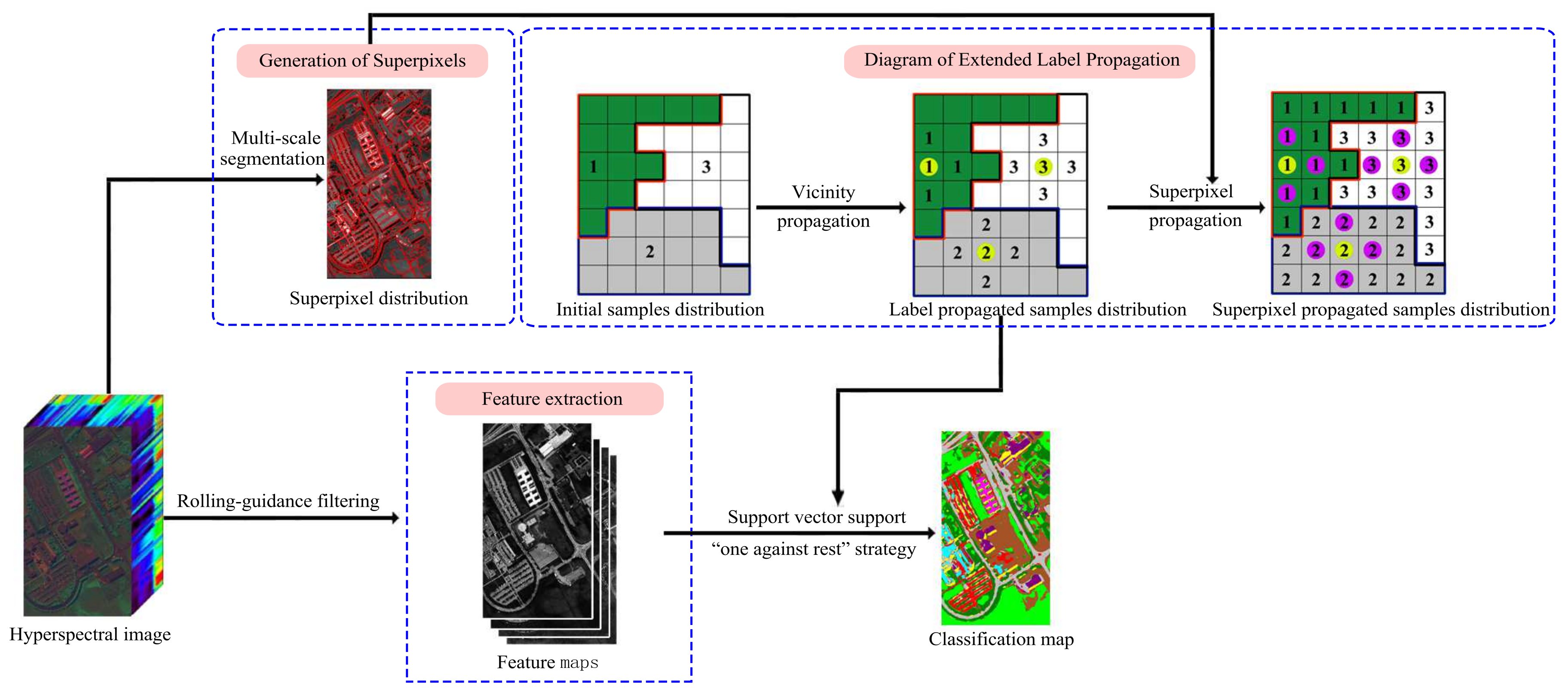
1. Superpixels segmentation:
      Obtain Y = ( Y 1 , , Y M ) , where Y i is the i-th superpixel, based on the multi-scale segmentation algorithm for X.
2. Extended label propagation method:
      Obtain the pseudo-labeled training sample set V ˜ n e w .
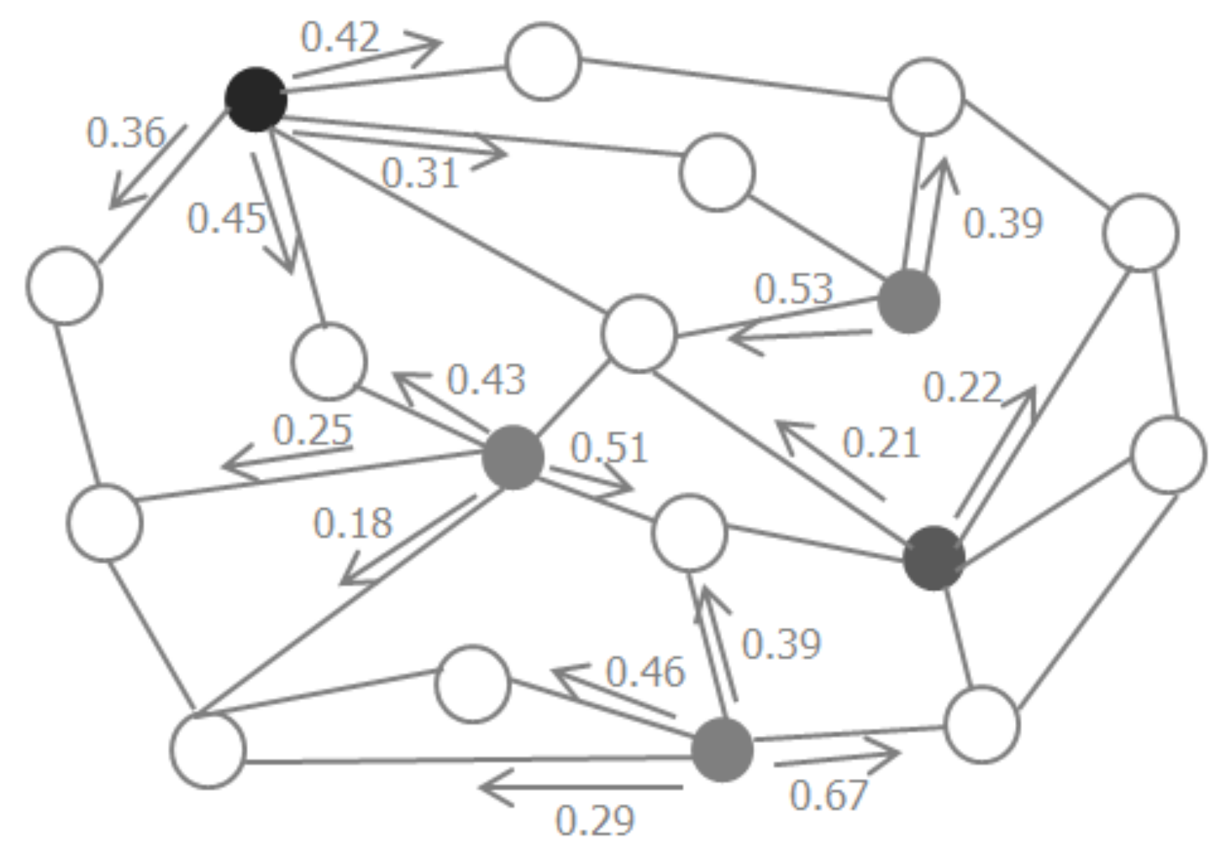
      (1) Label propagation:
               Selection of the unlabeled training set V U from the neighbors of the labeled samples.
               Construction of the weighted graph G and weighted matrix W i j by Equations (4)–(6).
               Calculation of the probability matrix P by Equations (7)–(10).
               Prediction of the labels of V U by Equation (11) and generation of the pseudo-labeled sample set V n e w .
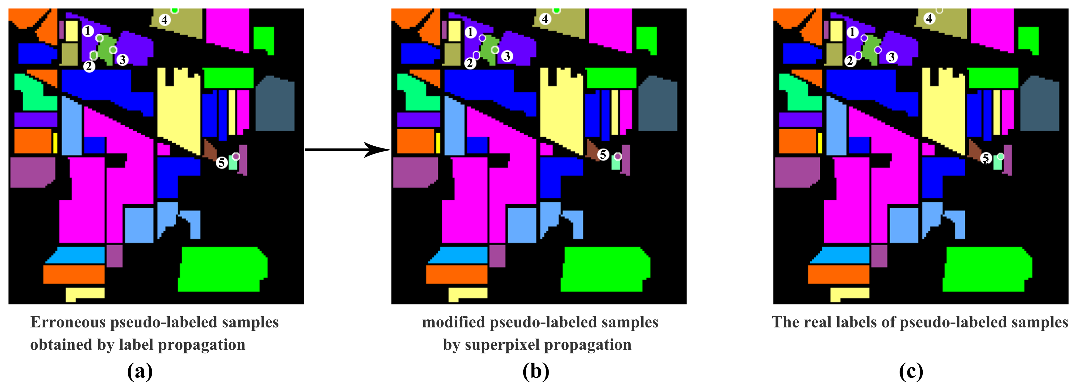
      (2) Superpixel propagation:
               Observation of the labels of labeled samples belonging to superpixel Y i , and then, the majority vote method is used to assign the labels for all pixels within Y i .
3. Rolling guidance filtering:
      Extraction of the spectral features of initial image X, and the filtered image I ˜ is obtained by Equations (10)–(12).
4. SVM classification:
       V L and V ˜ n e w are merged as the final training sample set, and then, train SVM to obtain the prediction of labels of the testing set. The input feature vector to the SVM is the filtered image by the rolling guidance filtering.
Note that we perform the SVM to obtain the final classification result, because it has a good performance for the non-linear problem [41]. The goal of SVM is to find an optimal decision hyperplane that can maximize the distance between the two nearest samples on the two sides of the plane for classification. In this paper, the “one against rest” strategy [42] is adopted to achieve the multi-classification.

4. Experiment

In this section, the experimental results are performed on three real hyperspectral datasets to evaluate the performance of the proposed ELP-RGF method.

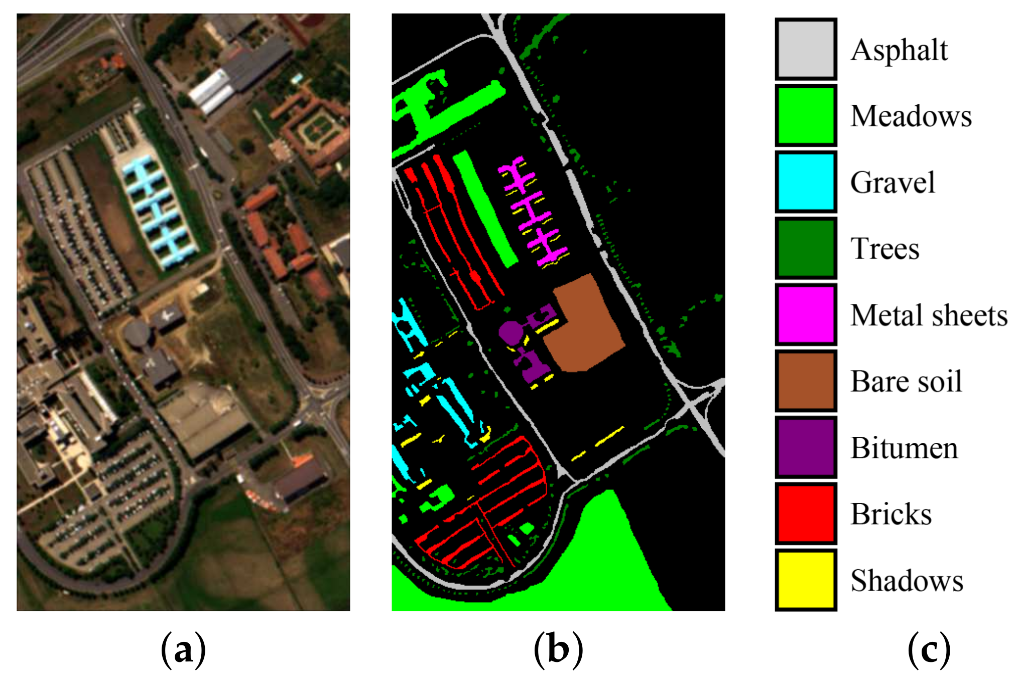
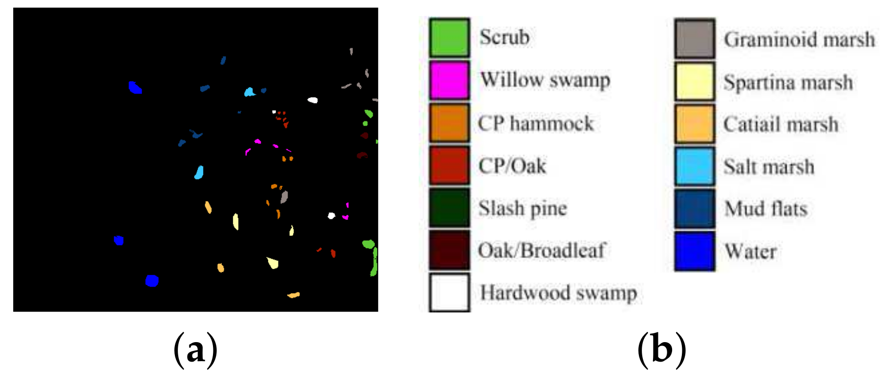
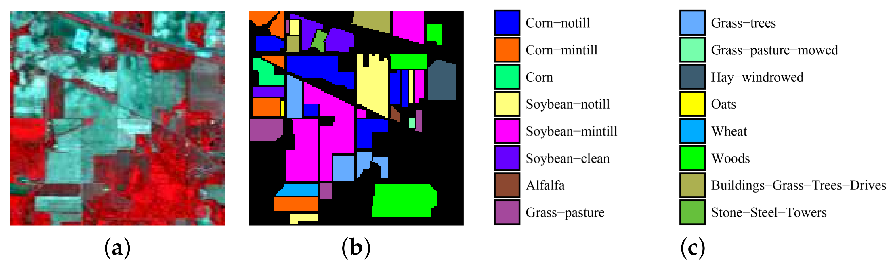
4.1. Datasets Description

In our experiments, three hyperspectral image datasets including the Indian Pines image, the University of Pavia image and the Kennedy Space Center image are utilized to evaluate the performance of the ELP-RGF.
(1) Indian Pines dataset: This image was acquired by the Airborne Visible/Infrared Imaging Spectrometer (AVIRIS) sensor, which captured an Indian Pines unlabeled agricultural site of northwestern Indiana and contains 220 × 145 × 145 bands. Twenty water absorption bands (Nos. 104–108, 150–163 and 220) were removed before hyperspectral image classification. The spatial resolution of the Indian Pines image is 20 m per pixel, and the spectral coverage ranges from 0.4–2.5 μ m. Figure 3 shows a color composite and the corresponding ground-truth data of the Indian Pines image.
(2) University of Pavia dataset: This image capturing the University of Pavia, Italy, was recorded by the Reflective Optics System Imaging Spectrometer (ROSIS). This image contains 115 bands and a size 610 × 340 with a spatial resolution of 1.3 m per pixel and a spectral coverage ranging from 0.43–0.86 μ m. Using a standard preprocessing approach before hyperspectral image classification, 12 noisy channels were removed. Nine classes of interest are considered for this image. Figure 4 shows the color composite and the corresponding ground-truth data of the University of Pavia image.
(3) Kennedy Space Center dataset: The Kennedy Space Center (KSC) image was captured by the National Aeronautics and Space Administration (NASA) Airborne Visible/Infrared Imaging Spectrometer instrument at a spatial resolution of 18 m per pixel. The KSC image contains 224 bands with a spatial size of 512 × 614, and the water absorption and low signal-to-noise ratio (SNR) bands were discarded before the classification. Figure 5 shows the KSC image and the corresponding ground-truth data.

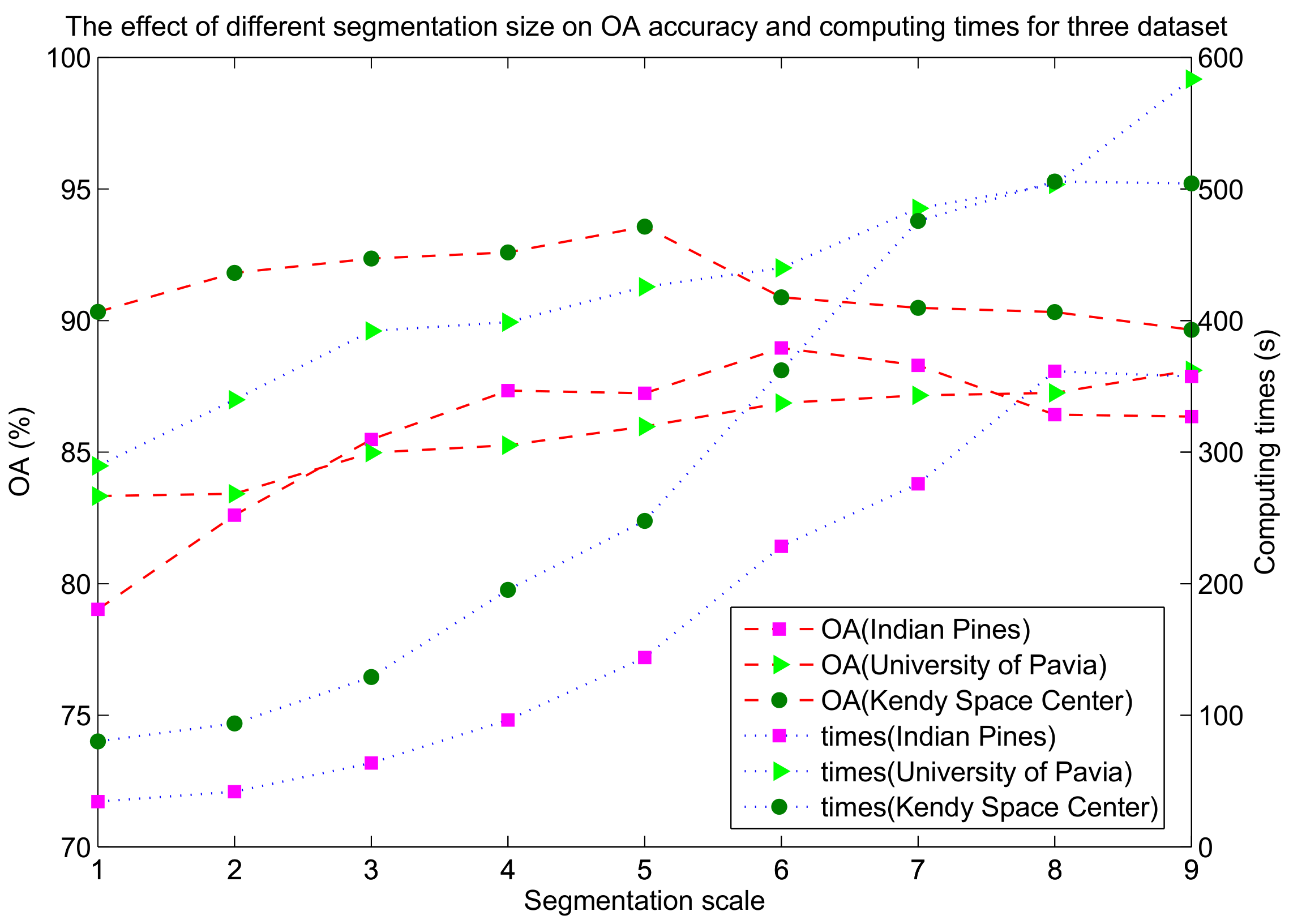
4.2. Parameter Analysis of the Proposed Method

In the experiments, the original images were segmented by the multi-scale segmentation method (MSS) [37]. In this section, we fix the shape parameters v = 0.1 and the smoothness parameter to u 1 = 0.5 in MSS. For the proposed method, there are three hyperparameters that have to be adjusted, namely weight parameter u, segmentation scale S and the width of spatial neighborhood d. The three hyperparameters were selected using the cross-validation strategy. Figure 6 shows the classification results obtained by the ELP-RGF method with different weight parameters μ and segmentation scales S. From Figure 6, we can see that the result of Figure 6a–b is visually more satisfactory than that of Figure 6c–d. If the process of label propagation entirely relied on the spatial graph, that is, u= 1 is applied, the result of ELP-RGF is poor, as Figure 6d shows. Therefore, μ = 0.001 to μ = 0.01 is considered the most optimal weight parameter range. We can see that the classification result of Figure 6f–g is better than Figure 6e,h, especially for the landscape of “Soybeans-min till“ and “Hay-windrowed“. In addition, Figure 7 shows the OA curves of ELP-RGF in the different u and dto illustrate the spatial weight parameter playing an important role in the process of label propagation. Furthermore, Figure 8 shows that the classification accuracies and computing time of the proposed method are significantly affected by S. When the two factors of the classification accuracy and the computing time are taken into full consideration (see Figure 8) and observing the selected parameters obtained by cross-validation, we can know that the optimal parameter range is 4–6.

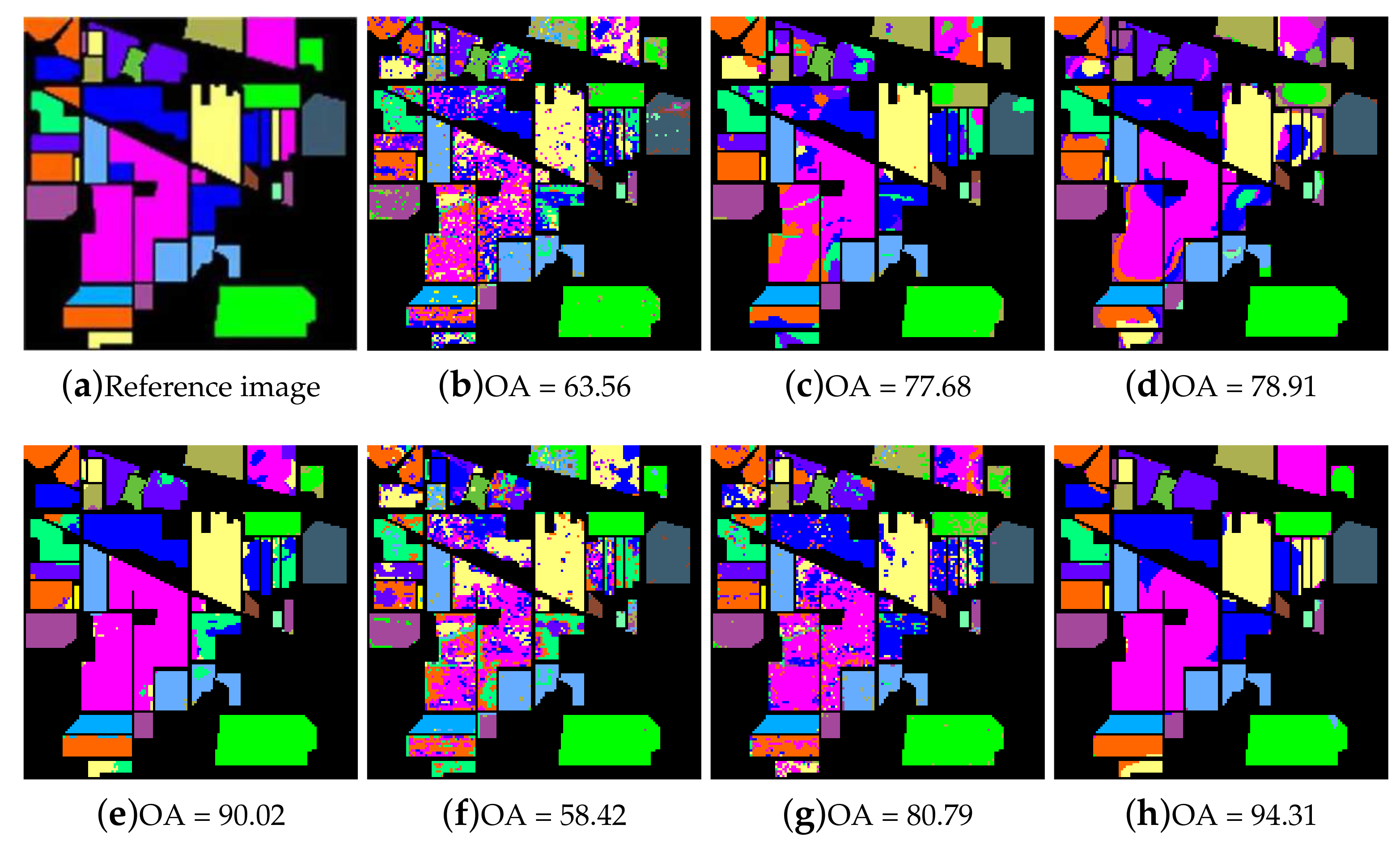
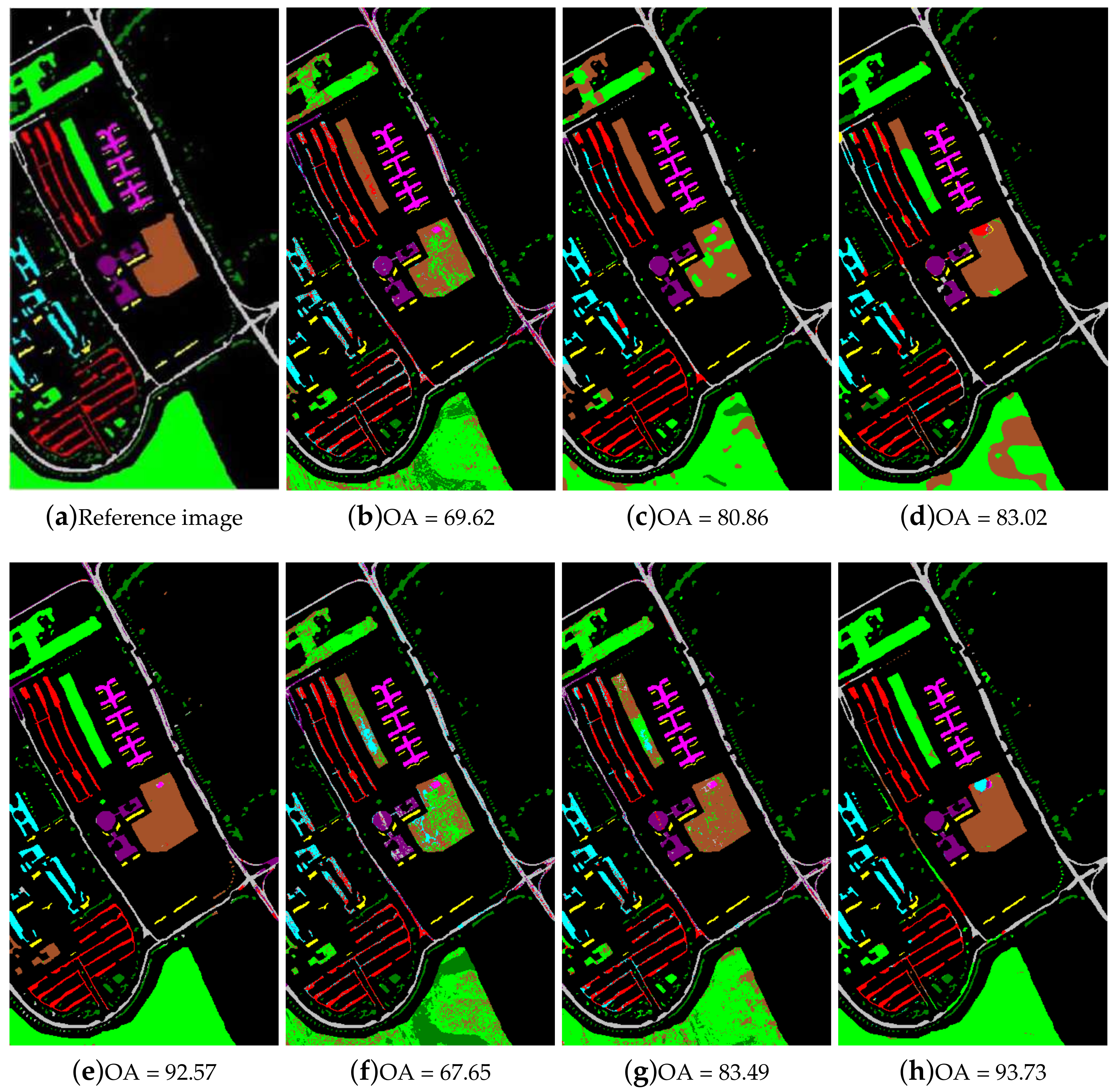
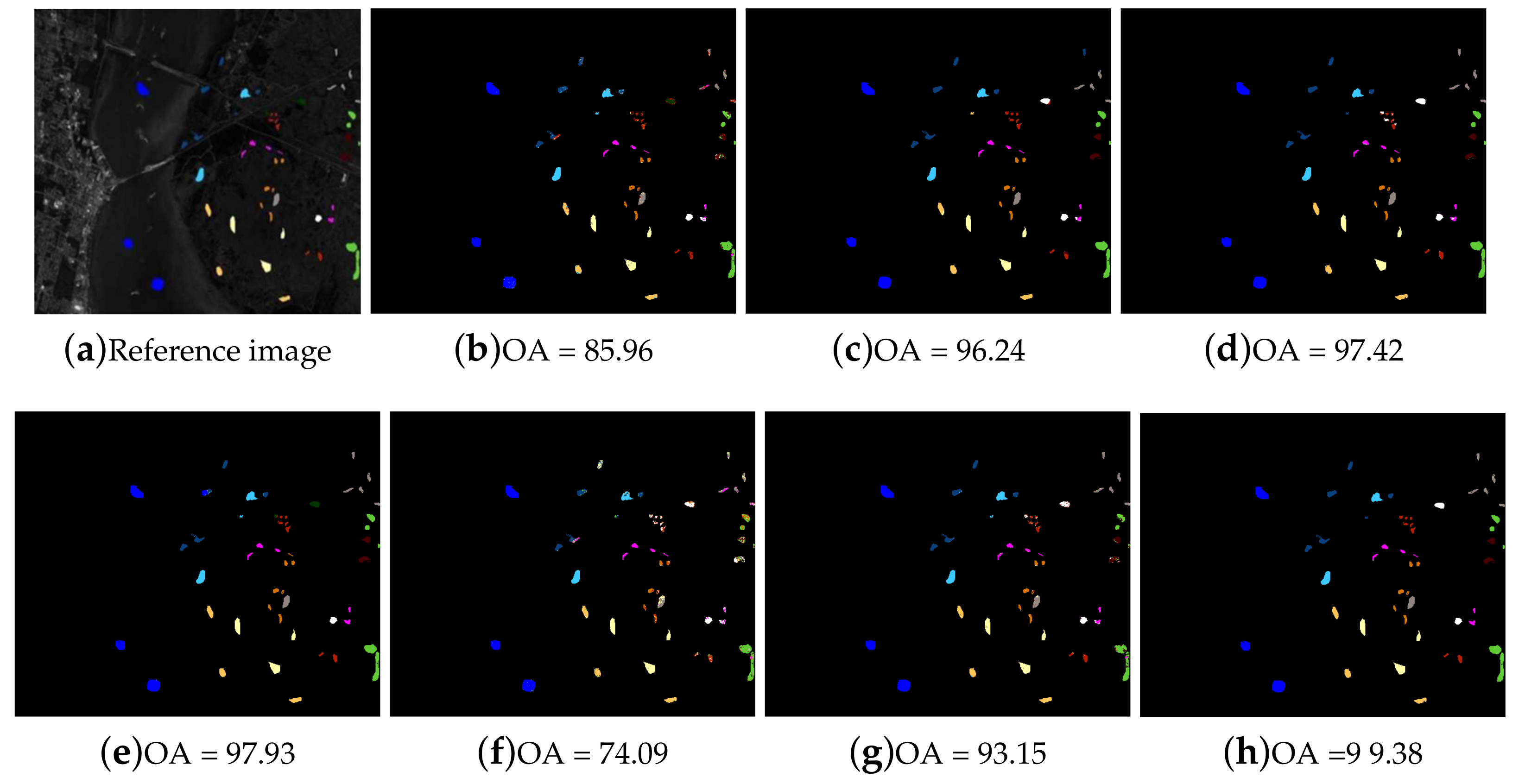
4.3. Comparison with Other Classification Methods

In this section, the proposed ELP-RGF method is compared with several hyperspectral image classification methods, i.e., the typical SVM method, more advanced extended random walkers (ERW) [43] and semi-supervised methods (the Laplacian support vector machine (LapSVM) [38] and spectral-spatial label propagation (SSLP-SVM) [24]). In addition, a post-processing-based edge-preserving filtering (EPF) [44] and the rolling guidance filtering method (RGF) [39] are also used as the comparison methods. The parameter settings for the EPF, ERW and SSLP-SVM methods are given in the corresponding papers. The evaluation indexes in Table 1, Table 2, Table 3 and Table 4 are given in the form of the mean ± standard deviation.
For the Indian Pines dataset, Table 1 shows the OA, AA and Kappa coefficient of different methods with the 5/10/15 training numbers per class (represented as s). From Table 1 we can see that the OA accuracy and Kappa coefficient of the proposed ELP-RGF method are better than other methods when the number of training samples is relatively small. In particular, when the s = 5, the OA accuracy of the proposed ELP-RGF method increases 14.29% and 36.63% compared to that of the SSLP-SVM method and the LapSVM method. The Kappa coefficient of ELP-RGF method is 13.52% higher than SSLP-SVM when s = 10, which fully shows the superiority of the two-step method proposed in this paper. We can see that the performance of the proposed ELP-RGF is always superior to that of the ERW method. As the number of training samples increases, the accuracy of the increase rate has decreased, however, there is still a large gap compared with other methods. Figure 9 shows the classification maps obtained by different methods. It can be seen that the classification map of the proposed method has less noise, and the boundary region in the classification map is also much clearer.
For the University of Pavia image, we randomly selected 5, 10 and 15 samples from each class as the training samples. Table 2 shows the OA, AA and Kappa coefficient of the different methods with different s. According to Table 2, the proposed ELP-RGF, SSLP-SVM, LapSVM and ERW can produce greater classification accuracy than the SVM at the same s. However, the degrees of the improvement of ERW, SSLP-SVM and LapSVM are smaller compared with ELP-RGF. For example, the OA of ERW and SSLP-SVM increased by 1.16% and 10.24%. The experimental result indicated that the proposed ELP-RGF outperforms the compared methods. The results show that the OA of the proposed method is 96.02%, which is 10.25% higher than that of the SSLP-SVM and 0.91% higher than that of the ERW when s = 15. The OA accuracy and kappa coefficients of the ELP-RGF method are always the highest, which demonstrates that the ELP-RGF is the most accurate classifier among these methods. We can see that compared with SVM, SSLP-SVM and ERW, the OA accuracy and Kappa coefficients of the ELP method are more competitive. Figure 10 shows the classification maps of different methods when s = 15. The figure shows the effectiveness of the proposed method. The proposed method presents more accurate classification results for the class of MetalSheetsand Gravel, and its classification result is better than those of other methods.
For the Kennedy Space Center dataset, we evaluated the classification accuracies of different methods using 39 training samples collected from each class. Table 3 shows the OAs, AAs, Kappa and individual classification accuracies obtained for the various methods. From Table 3, it is demonstrated that the OA, AA and Kappa accuracy of the proposed method are the highest in all comparative methods. Most of individual accuracies are significantly higher than other methods. For the class of Willowswamp, the accuracies of the proposed method and SSLP-SVM are 99.75% and 77.38%; thus, the accuracy gain is 22.37%. For the class of Oak/Broadleaf, the proposed method can produce 59.21% and 57.11% OA improvements compared with SSLP-SVM and SVM. Table 4 provides the OA accuracies of the various methods. Observing the values in Table 4, we can see that the classification accuracy is proportional to s. Moreover, the performance of the proposed method is not only higher than the other semi-supervised classification methods, but also can improve more than that of ERW. Figure 11 shows that the proposed ELP-RGF method can achieve better classification performance and produce little noise compared with other methods.
Table 5 lists the number of samples generated by the two semi-supervised methods (i.e., SSLP-SVM and ELP-RGF) under three different datasets and the correct rate of these new labeled samples. We can see that the total number of labeled samples generated by the ELP-RGF method is almost 7–22-times more than that generated by the SSLP-SVM method for three datasets. Although the correct rate of the SSLP-SVM method is slightly higher, the ELP-RGF method is also competitive. More importantly, the proposed ELP-RGF can produce more labeled samples.
Table 6 illustrates the effect of the superpixel by comparing with the RGF method, the combination of label propagation and RGF and the combination of superpixel propagation and RGF. The table shows that the superpixel propagation plays a major role in the proposed method. For example, for the Indian Pines image, the OA accuracy of the proposed ELP-RGF is 79.13%, while the accuracy obtained by SP-RGF and RGF is 75.62% and 56.14%, respectively. For the Kennedy Space Center image, the OA accuracy of the SP-RGF method is 4.64% higher than that of LP-RGF. As Table 6 shows, the accuracy of the SL-RGF is more than that of the LP-RGF method when RGF is used in those methods. While LP-RGF is higher than SP-RGF, the gap is small. Thus, the process of superpixel propagation is very useful to help improve the classification result.

5. Discussion

In this paper, the proposed ELP-RGF method is used to increase the number of training samples and optimize the features of the initial hyperspectral image. Previous label propagation-based works, such as SSLP-SVM, only increased a small number of training samples, which are neighboring the labeled samples, and the computational expense is large. If the scope of propagation is beyond neighbors, the computing time will rapidly increase. Furthermore, in the process of label propagation, some wrongly-labeled samples may be introduced to train the model, resulting in misclassification. In our ELP-RGF method, a two-step label prorogation process called ELP is proposed, which first utilized the spatial-spectral label propagation to propagate the label information from labeled samples to the neighboring unlabeled samples. Then, superpixel propagation is used to expand the scope of propagation to the entire superpixel to increase the huge number of training samples, and it is less time consuming compared to the propagation beyond neighbors. Compared with other semi-supervised classification methods, ELP has two obvious advantages: on the one hand, it can generate a large number of pseudo-labeled samples for model training; on the other hand, it can ensure the ‘effectiveness’ of the increased pseudo-labeled samples; here, ‘effectiveness’ means that almost all of the labels of the pseudo-labeled samples are correct, which was shown in Table 6. Moreover, as shown in Figure 12, the wrongly-labeled samples in the first step of the ELP method can be modified by the superpixel propagation. Thus, the proposed ELP-RGF method shows a better classification performance than other comparative methods. However, the greatest limitation of the proposed method is that the classification result is over-reliant on the segmentation scale. As shown in Figure 8, the difference in classification results with different segmentation scales is larger.

6. Conclusions

In this paper, a novel semi-supervised classification method of hyperspectral images based on extended label propagation and rolling guidance filtering is proposed. The first advantage of this method is that the number of pseudo-labeled training samples is significantly increased. The second advantage is that the diversity of training samples is improved to enhance the generalization of the proposed method. The third advantage is that the spatial information is fully considered using graphs and superpixels. The experimental results on three different hyperspectral datasets demonstrate that the proposed ELP-RGF method offers an excellent performance in terms of both visual quality and quantitative evaluation indexes. In particular, when the number of training samples is relatively small, the improvement is more obvious.

Acknowledgments

This work was co-supported by the National Natural Science Foundation of China (NSFC) (41406200, 61701272) and Shandong Province Natural Science Foundation of China (ZR2014DQ030, ZR2017PF004).

Author Contributions

Binge Cui conceived of the idea of this paper. Xiaoyun Xie designed the experiments and drafted the paper. Binge Cui, Siyuan Hao, Jiandi Cui and Yan Lu revised the paper.

Conflicts of Interest

The authors declare no conflict of interest.

References

  1. Zhong, Z.; Fan, B.; Duan, J.; Wang, L.; Ding, K.; Xiang, S. Discriminant Tensor Spectral–Spatial Feature Extraction for Hyperspectral Image Classification. IEEE Geosci. Remote Sens. Lett. 2017, 12, 1028–1032. [Google Scholar] [CrossRef]
  2. Xu, X.; Shi, Z. Multi-objective based spectral unmixing for hyperspectral images. ISPRS J. Photogramm. Remote Sens. 2017, 124, 54–69. [Google Scholar]
  3. Zhang, L.; Zhang, L.; Tao, D.; Huang, X. Sparse Transfer Manifold Embedding for Hyperspectral Target Detection. IEEE Geosci. Remote Sens. Lett. 2013, 52, 1030–1043. [Google Scholar]
  4. Pan, B.; Shi, Z.; An, Z.; Jiang, Z.; Ma, Y. Sparse Transfer Manifold Embedding for Hyperspectral Target Detection. IEEE J. Sel. Top. Appl. Earth Obs. Remote Sens. 2017, 99, 1–13. [Google Scholar]
  5. Kang, X.; Zhang, X.; Li, S.; Li, K.; Li, J.; Benediktsson, J.A. Hyperspectral Anomaly Detection with Attribute and Edge-Preserving Filters. IEEE Trans. Geosci. Remote Sens. 2017, 99, 1–12. [Google Scholar] [CrossRef]
  6. Chang, C.I. Hyperspectral Imaging: Techniques for Spectral Detection and Classification; Plenum Publishing Co.: New York, NY, USA, 2003. [Google Scholar]
  7. Hughes, G. On the mean accuracy of statistical pattern recognizers. Inf. Theory IEEE Trans. 1968, 14, 55–63. [Google Scholar] [CrossRef]
  8. Gotsis, P.K.; Chamis, C.C.; Minnetyan, L. Classification of hyperspectral remote sensing images with support vector machines. IEEE Trans. Geosci. Remote Sens. 2004, 42, 1778–1790. [Google Scholar]
  9. Benediktsson, J.A.; Swain, P.H.; Ersoy, O.K. Neural Network Approaches versus Statistical Methods in Classification of Multisource Remote Sensing Data. Geosci. Remote Sens. Symp. 1989, 28, 540–552. [Google Scholar] [CrossRef]
  10. Xia, J.; Du, P.; He, X.; Chanussot, J. Hyperspectral Remote Sensing Image Classification Based on Rotation Forest. IEEE Geosci. Remote Sens. Lett. 2013, 11, 239–243. [Google Scholar] [CrossRef]
  11. Chen, Y.; Jiang, H.; Li, C.; Jia, X.; Ghamisi, P. Deep Feature Extraction and Classification of Hyperspectral Images Based on Convolutional Neural Networks. IEEE Trans. Geosci. Remote Sens. 2016, 54, 6232–6251. [Google Scholar] [CrossRef]
  12. Fauvel, M.; Tarabalka, Y.; Benediktsson, J.A.; Chanussot, J.; Tilton, J.C. Advances in Spectral-Spatial Classification of Hyperspectral Images. Proc. IEEE. 2013, 101, 652–675. [Google Scholar] [CrossRef]
  13. Pan, B.; Shi, Z.; Xu, X. R-VCANet: A New Deep-Learning-Based Hyperspectral Image Classification Method. IEEE J. Sel. Top. Appl. Earth Obs. Remote Sens. 2017, 99, 1–12. [Google Scholar] [CrossRef]
  14. Kang, X.; Xiang, X.; Li, S.; Benediktsson, J.A. PCA-Based Edge-Preserving Features for Hyperspectral Image Classification. IEEE Trans. Geosci. Remote Sens. 2017, 99, 1–12. [Google Scholar] [CrossRef]
  15. Pan, B.; Shi, Z.; Xu, X. MugNet: Deep learning for hyperspectral image classification using limited samples. ISPRS J. Photogramm. Remote Sens. 2017. [Google Scholar] [CrossRef]
  16. Pan, B.; Shi, Z.; Xu, X. Hierarchical Guidance Filtering-Based Ensemble Classification for Hyperspectral Images. IEEE Trans. Geosci. Remote Sens. 2017, 99, 1–13. [Google Scholar] [CrossRef]
  17. Pan, B.; Shi, Z.; Zhang, N.; Xie, S. Hyperspectral Image Classification Based on Nonlinear Spectral–Spatial Network. IEEE Geosci. Remote Sens. Lett. 2016, 99, 1–5. [Google Scholar] [CrossRef]
  18. Camps-Valls, G.; Marsheva, T.V.B.; Zhou, D. Semi-Supervised Graph-Based Hyperspectral Image Classification. IEEE Trans. Geosci. Remote Sens. 2007, 45, 3044–3054. [Google Scholar] [CrossRef]
  19. Shao, Y.; Sang, N.; Gao, C. Probabilistic Class Structure Regularized Sparse Representation Graph for Semi-Supervised Hyperspectral Image Classification. Pat. Recognit. 2017, 63, 102–114. [Google Scholar] [CrossRef]
  20. Krishnapuram, B.; Carin, L.; Figueiredo, M.A.T.; Member, S. Sparse multinomial logistic regression: Fast algorithms and generalization bounds. IEEE Trans. Pat. Anal. Mach. Intell. 2005, 27, 957–968. [Google Scholar] [CrossRef] [PubMed]
  21. Ando, R.K.; Zhang, T. Two-view feature generation model for semi-supervised learning. In Proceedings of the International Conference on Machine Learning, Corvalis, OR, USA, 20–24 June 2007. [Google Scholar]
  22. Meng, J.; Jung, C. Semi-Supervised Bi-Dictionary Learning for Image Classification With Smooth Representation-Based Label Propagation. IEEE Transa. Multimedia. 2016, 18, 458–473. [Google Scholar]
  23. Wang, F.; Zhang, C. Label Propagation through Linear Neighborhoods. IEEE Trans. Knowl. Data Eng. 2008, 20, 55–67. [Google Scholar] [CrossRef]
  24. Wang, L.; Hao, S.; Wang, Q.; Wang, Y. Semi-supervised classification for hyperspectral imagery based on spatial-spectral Label Propagation. Isprs J. Photogramm. Remote Sens. 2014, 97, 123–137. [Google Scholar] [CrossRef]
  25. Zhu, X.; Ghahramani, Z.; Mit, T.J. Semi-Supervised Learning with Graphs. In Proceedings of the International Joint Conference on Natural Language Processing, Carnegie Mellon University, Pittsburgh, PA, USA, January 2005; pp. 2465–2472. [Google Scholar]
  26. Cheng, H.; Liu, Z. Sparsity induced similarity measure for label propagation. In Proceedings of the IEEE International Conference on Computer Vision, Kyoto, Japan, 29 September–2 October 2009. [Google Scholar]
  27. Karasuyama, M.; Mamitsuka, H. Multiple Graph Label Propagation by Sparse Integration. IEEE Trans. Neural Netw. Learn. Syst. 2013, 24, 1999–2012. [Google Scholar] [CrossRef] [PubMed]
  28. Zhu, X.; Ghahramani, Z. Semi-Supervised Learning Using Gaussian Fields and Harmonic Functions. In Proceedings of the Twentieth International Conference on International Conference on Machine Learning, Washington, DC, USA, 21–24 August 2003. [Google Scholar]
  29. Moore, A.P.; Prince, S.J.D.; Warrell, J.; Mohammed, U. Superpixel lattices. In Proceedings of the Computer Vision and Pattern Recognition, Anchorage, AK, USA, 23–28 June 2008. [Google Scholar]
  30. Wang, L.; Zhang, J.; Liu, P.; Choo, K.K.R.; Huang, F. Spectral-spatial multi-feature-based deep learning for hyperspectral remote sensing image classification. Soft Comput. A Fusion Found. Methodol. Appl. 2017, 21, 213–221. [Google Scholar] [CrossRef]
  31. Zhang, S.; Li, S.; Fu, W.; Fang, L. Multiscale Superpixel-Based Sparse Representation for Hyperspectral Image Classification. Remote Sens. 2017, 9, 139. [Google Scholar] [CrossRef]
  32. Achanta, R.; Shaji, A.; Smith, K.; Lucchi, A.; Fua, P.; Süsstrunk, S. SLIC Superpixels; EPFL: Lausanne, Switzerland, 2010. [Google Scholar]
  33. De Carvalho, M.A.G.; da Costa, A.L.; Ferreira, A.C.B.; Junior, R.M.C. Image Segmentation Using Watershed and Normalized Cut. In Proceedings of the SIBIGRAPI, Gramado, Brazil, 30 August–3 September 2009. [Google Scholar]
  34. Ugarriza, L.G.; Saber, E.; Vantaram, S.R.; Amuso, V.; Shaw, M.; Bhaskar, R. Automatic image segmentation by dynamic region growth and multiresolution merging. IEEE Trans. Image Process. Publ. IEEE Signal Process. Soc. 2009, 18, 2275–2288. [Google Scholar] [CrossRef] [PubMed]
  35. Jin, X.; Gu, Y. Superpixel-Based Intrinsic Image Decomposition of Hyperspectral Images. IEEE Trans. Geosci. Remote Sens. 2017, 99, 1–11. [Google Scholar]
  36. Jia, S.; Deng, B.; Zhu, J.; Jia, X.; Li, Q. Superpixel-Based Multitask Learning Framework for Hyperspectral Image Classification. IEEE Trans. Geosci. Remote Sens. 2017, 99, 1–14. [Google Scholar] [CrossRef]
  37. Zhang, D.; Yang, Y.; Song, K. Research on a Multi-Scale Segmentation Algorithm Based on High Resolution Satellite Remote Sensing Image. International Conference on Intelligent Control and Computer Application. 2016.
  38. Belkin, M.; Niyogi, P.; Sindhwani, V. Manifold regularization: A geometric framework for learning from labeled and unlabeled examples. Mach. Learn. Res. 2006, 7, 2399–2434. [Google Scholar]
  39. Zhang, Q.; Shen, X.; Xu, L. Rolling Guidance Filter. In Proceedings of the European Conference on Computer Vision, Zurich, Switzerland, 6–12 September 2014. [Google Scholar]
  40. Rohban, M.H.; Rabiee, H.R. Supervised neighborhood graph construction for semi-supervised classification. Pat. Recognit. 2012, 4, 1363–1372. [Google Scholar] [CrossRef]
  41. Vapnik, V.N. The Nature of Statistical Learning Theory. IEEE Trans. Neural Netw. 1997, 8, 1564. [Google Scholar]
  42. Wang, L.; Zhang, Y.; Gu, Y. The research of simplification of structure of multiclass classifier of support vector machine. Image Graph. 2005, 5, 571–572. [Google Scholar]
  43. Kang, X.; Li, S.; Fang, L.; Li, M.; Benediktsson, J.A. Extended Random Walker-Based Classification of Hyperspectral Images. IEEE Trans. Geosci. Remote Sens. 2014, 53, 144–153. [Google Scholar] [CrossRef]
  44. Kang, X.; Li, S.; Benediktsson, J.A. Spectral–Spatial Hyperspectral Image Classification With Edge-Preserving Filtering. IEEE Trans. Geosci. Remote Sens. 2014, 52, 2666–2677. [Google Scholar] [CrossRef]
Figure 1. Procedure of label propagation.
Remotesensing 10 00515 g001
Figure 2. Schematic of the proposed semi-supervised classification method of hyperspectral images based on extended label propagation and rolling guidance filtering.
Remotesensing 10 00515 g002
Figure 3. Indian Pines dataset. (a) False-color composite; (b,c) Ground-truth data.
Remotesensing 10 00515 g003
Figure 4. University of Pavia image. (a) False-color composite; (b,c) Ground-truth data.
Remotesensing 10 00515 g004
Figure 5. (a,b) Ground truth data of the Kennedy Space Center images.
Remotesensing 10 00515 g005
Figure 6. The analysis for the hyperparameters μ and S for the Indian Pines image. In the first row, S is fixed as five. (ad) respectively showthe classification results obtained by the extended label propagation (ELP)-RGF method with (a) u = 0.001, (b) u = 0.01, (c) u = 0.1 and (d) u = 1. In the second row, μ is fixed as 0.01; (eh) respectively showthe classificationmaps obtained by ELP-RGFmethodwith (e) S = 1, (f) S = 3, (g) S = 5 and (h) S = 9.
Remotesensing 10 00515 g006
Figure 7. Influence of μ and d on the Kappa coefficient of ELP-RGF for the Indian Pines dataset.
Remotesensing 10 00515 g007
Figure 8. The effect of the different segmentation size on OA accuracy and computing times for three datasets.
Remotesensing 10 00515 g008
Figure 9. Classification maps of different methods for the Indian Pines image. (a) Reference image; (b) SVM method; (c) EPF method; (d) RGF method; (e) ERW method; (f) LapSVM method; (g) SSLP-SVM method and (h) ELP-RGF method.
Remotesensing 10 00515 g009
Figure 10. Classification maps of different methods for the University of Pavia image (a) Reference image; (b) SVM method; (c) EPF method; (d) RGF method; (e) ERWmethod; (f) LapSVM method; (g) SSLP-SVM method and (h) ELP-RGF method.
Remotesensing 10 00515 g010
Figure 11. Classification maps of different methods for the Kennedy Space Center image. (a) Reference image; (b) SVM method; (c) EPF method; (d) RGF method; (e) ERW method; (f) LapSVM method; (g) SSLP-SVM method; (h) ELP-RGF method.
Remotesensing 10 00515 g011
Figure 12. The process of modifying the wrongly-labeled samples. (a) The five wrongly-labeled pseudo-labeled samples are provided; (b) shows that the first and second labels of pseudo-labeled have been modified by superpixel propagation; (c) shows the real labels of the provided wrongly-labeled pseudo-labeled samples.
Remotesensing 10 00515 g012
Table 1. Comparison of classification accuracies (in percentage) provided by different methods using different training samples per class (Indian Pines image). EPF, edge-preserving filtering; ERW, extended random walkers; LapSVM, Laplacian SVM; SSLP, spectral-spatial label propagation.
MethodsMetricsTraining Samples per Class (s)
s = 5s = 10s = 15
SVMOA45.31 ± 5.1957.58 ± 2.9863.56 ± 2.61
AA47.41 ± 3.7155.19 ± 2.2759.84 ± 2.21
Kappa39.21 ± 5.4352.52 ± 3.1759.11 ± 2.82
EPFOA57.97 ± 5.9369.89 ± 3.4577.68 ± 3.08
AA61.35 ± 6.4070.07 ± 3.4779.58 ± 2.70
Kappa52.91 ± 6.5066.12 ± 3.7774.80 ± 3.45
RGFOA56.14 ± 5.3370.49 ± 4.6978.91 ± 1.39
AA61.18 ± 4.8968.49 ± 5.0374.52 ± 2.77
Kappa51.13 ± 5.8266.89 ± 5.0876.14 ± 1.55
ERWOA72.30 ± 4.3884.87 ± 4.4190.02 ± 1.30
AA83.32 ± 2.4191.48 ± 2.3094.39 ± 0.94
Kappa68.96 ± 4.6982.95 ± 4.8688.69 ± 1.46
LapSVMOA42.50 ± 0.2758.58 ± 0.4658.42 ± 0.32
AA50.96 ± 1.3661.54 ± 0.2662.20 ± 0.86
Kappa36.89 ± 0.5453.01 ± 0.3253.82 ± 0.36
SSLP-SVMOA64.84 ± 1.4376.05 ± 0.7380.79 ± 1.44
AA65.96 ± 2.3878.07 ± 0.6482.08 ± 0.98
Kappa60.63 ± 1.4973.17 ± 0.8078.38 ± 1.60
ELP-RGFOA79.13 ± 1.8089.14 ± 1.0694.31 ± 0.75
AA77.65 ± 2.9488.98 ± 1.3794.45 ± 1.54
Kappa76.37 ± 2.0387.68 ± 1.2093.53 ± 0.85
Table 2. Overall accuracy of the various methods for the University of Pavia image (average of 10 runs with thestandard deviation; the bold values indicate the greatest accuracy among the methods in each case).
Methods = 5s = 10s = 15
SVM61.54 ± 5.1567.70 ± 4.7269.62 ± 3.35
EPF58.98 ± 8.5871.07 ± 8.0280.86 ± 6.37
RGF55.85 ± 7.2274.82 ± 4.4983.02 ± 4.87
ERW80.70 ± 6.4590.28 ± 3.7192.57 ± 4.36
LapSVM62.23 ± 2.0363.03 ± 0.2267.65 ± 0.43
SSLP-SVM67.15 ± 2.4582.15 ± 0.7183.49 ± 1.30
ELP-RGF82.39 ± 1.4291.54 ± 1.5493.73 ± 1.37
Table 3. Individual class accuracies, OA, AA and Kappa coefficient (in percentage) for the Kennedy Space Center images.
ClassTrainingTestAccuracy of Classification
SVMEPFRGFERWLapSVMSSLP-SVMELP-RGF
Scrub375892.25 ± 6.1590.55 ± 2.2596.78 ± 6.9288.68 ± 17.9987.17 ± 6.1387.19 ± 6.27100
Willow swamp324072.87 ± 9.3886.74 ± 1.4781.32 ± 14.7868.56 ± 20.1395.63 ± 0.6977.38 ± 4.5999.75 ± 0.30
CP hammock325370.65 ± 9.0287.00 ± 2.3675.16 ± 19.6762.70 ± 23.8470.90 ± 2.8585.87 ± 6.5693.06 ± 5.65
CP/Oak324935.41 ± 9.2354.50 ± 2.2637.26 ± 18.7177.10 ± 22.4583.97 ± 10.3251.97 ± 16.9275.49 ± 22.72
Slash pine315843.04 ± 10.7459.64 ± 3.0146.26 ± 39.5688.29 ± 8.8179.08 ± 1.6041.13 ± 8.2955.95 ± 4.09
Oak/Broadleaf322638.53 ± 18.2362.16 ± 3.0458.85 ± 43.7894.48 ± 15.4489.62 ± 3.2736.43 ± 9.4695.64 ± 3.89
Hardwood swamp310252.88 ± 17.1877.62 ± 1.6580.03 ± 20.8010096.34 ± 1.1872.06 ± 10.9598.79 ± 1.15
Graminoid marsh342843.90 ± 16.0966.50 ± 2.0367.77 ± 37.2576.09 ± 21.6193.34 ± 1.2676.47 ± 11.1199.10 ± 0.74
Spartina marsh351775.42 ± 10.3081.25 ± 2.1285.19 ± 12.8978.86 ± 19.2598.12 ± 0.6789.52 ± 3.2197.21 ± 3.90
Cattail marsh340159.72 ± 28.9672.09 ± 2.7361.39 ± 43.0272.13 ± 23.0592.90 ± 9.7775.53 ± 13.8784.79 ± 17.69
Salt marsh341689.04 ± 23.0190.09 ± 2.4289.94 ± 24.6485.56 ± 22.8294.92 ± 4.0784.47 ± 16.3499.95 ± 0.10
Mud flats350067.62 ± 16.5778.70 ± 2.3989.86 ± 14.4973.77 ± 26.2594.22 ± 2.2568.16 ± 7.8294.21 ± 4.38
Water392498.58 ± 2.3598.90 ± 0.5983.33 ± 40.8293.36 ± 16.7499.08 ± 0.7299.15 ± 0.78100
OA65.45 ± 8.1276.13 ± 0.9666.81 ± 7.8782.21 ± 4.3691.25 ± 1.1875.52 ± 1.2493.21 ± 2.44
AA64.61 ± 4.1077.36 ± 0.6873.32 ± 4.5681.51 ± 3.5990.41 ± 0.8172.72 ± 1.1891.84 ± 2.23
Kappa61.76 ± 8.7673.52 ± 1.0263.52 ± 8.4480.25 ± 4.7990.25 ± 1.3272.88 ± 1.3592.45 ± 2.71
Table 4. Overall accuracy of the various methods for the Kennedy Space Center image (average of 10 runs with thestandard deviation; the bold values indicate the greatest accuracy among the method in each case).
Methods = 5s = 10s = 15
SVM74.05 ± 3.6583.12 ± 1.8385.96 ± 1.31
EPF85.48 ± 4.2692.66 ± 2.8296.24 ± 1.87
RGF87.05 ± 4.3295.30 ± 1.7697.42 ± 1.51
ERW88.29 ± 3.1996.85 ± 1.3797.93 ± 0.94
LapSVM61.40 ± 0.1271.94 ± 0.1074.09 ± 0.30
SSLP-SVM82.01 ± 2.9390.61 ± 0.9093.15 ± 0.53
ELP-RGF94.12 ± 0.6599.05 ± 0.2499.38 ± 0.12
Table 5. Correct rate of samples generated by the two semi-supervised methods of three datasets.
MethodsData SetInitial SamplesIncreased SamplesIncorrect Labeled SamplesCorrect Rate
SSLP-SVMIndian Pines108349199.71%
University of Pavia901028499.61%
Kennedy Space Center391150100%
ELP-RGFIndian Pines10829982599.17%
University of Pavia907440999.88%
Kennedy Space Center3925582599.02%
Table 6. Overall accuracy of the various combined methods involved in the proposed method for three datasets.
Data SetRGFLP-RGFSP-RGFELP-RGF
Indian Pines56.1467.6375.6279.13
University of Pavia55.8575.2274.2582.39
Kennedy Space Center87.0589.3393.9794.12

