An Automatic Sparse Pruning Endmember Extraction Algorithm with a Combined Minimum Volume and Deviation Constraint


1
College of Electrical and Information Engineering, Hunan University, Changsha 410082, Hunan, China
2
Shenzhen Institutes of Advanced Technology, Chinese Academy of Sciences, Shenzhen 518055, Guangdong, China
3
Center for Assessment and Development of Real Estate, Shenzhen 518040, Guangdong, China
*
Author to whom correspondence should be addressed.
Remote Sens. 2018, 10(4), 509; https://doi.org/10.3390/rs10040509
Submission received: 24 January 2018
/
Revised: 14 March 2018
/
Accepted: 21 March 2018
/
Published: 23 March 2018
(This article belongs to the Section Remote Sensing Image Processing)
Abstract
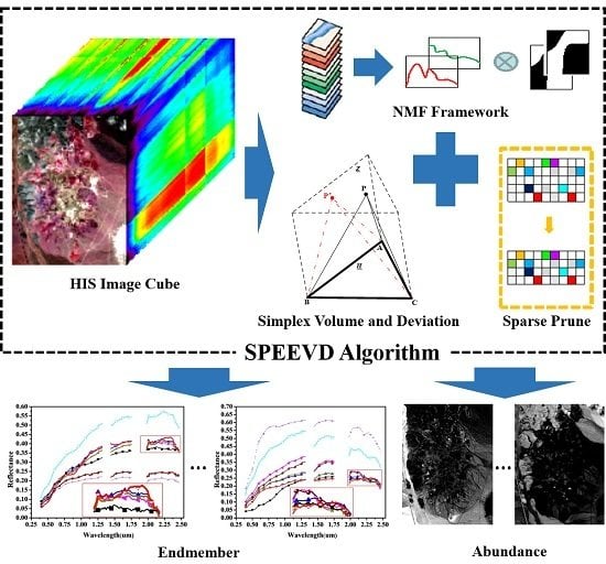
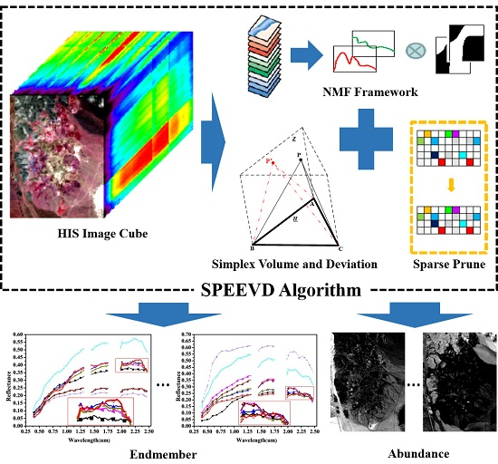
:In this paper, an automatic sparse pruning endmember extraction algorithm with a combined minimum volume and deviation constraint (SPEEVD) is proposed. The proposed algorithm can adaptively determine the number of endmembers through a sparse pruning method and, at the same time, can weaken the noise interference by a minimum volume and deviation constraint. A non-negative matrix factorization solution based on the projection gradient is mathematically applied to solve the combined constrained optimization problem, which makes sure that the convergence is steady and robust. Experiments were carried out on both simulated data sets and real AVIRIS data sets. The experimental results indicate that the proposed method does not require a predetermined endmember number, but it still manifests an improvement in both the root-mean-square error (RMSE) and the endmember spectra, compared to the other state-of-the-art methods, most of which need an accurate pre-estimation of endmember number.
1. Introduction
Much research has been under taken on remotely sensed hyperspectral data processing in recent years, covering topics such as dimensionality reduction [1,2,3], classification [4,5], target detection [6,7,8], data compression [9,10], and spectral unmixing [11,12,13,14,15,16,17,18,19]. Most of this research assumes that each pixel vector comprises the response of a single underlying material in the scene. However, if the spatial resolution of the sensor is low, different materials may jointly occupy a single pixel [14]. The resulting spectral measurement will be a mixed pixel, composed of the individual pure spectra (i.e., endmembers) and their corresponding fractional abundances [13,14].
According to the assumption as to whether pure pixels exist in the image, endmember extraction methods can be classified into two groups: endmember identification [20] and endmember generation [14]. Endmember identification is based on the assumption that the input data set contains at least one pure pixel for each distinct material present in the scene. Many methods with this assumption have achieved promising performance [21,22,23,24,25,26,27,28]. They search for the purest pixel for a given endmember if the pixel performs as a vertex in the simplex. A typical method, such as the pixel purity index [21], aims at finding the most spectrally pure signatures in the imaging scene by a large number of projections. Other typical endmember identification methods include the N-finder algorithm (N-FINDR) [24], vertex component analysis (VCA) [25], the simplex growing algorithm (SGA) [26] and its extension [27], and the automatic morphological endmember extraction (AMEE) [28]. However, the assumption behind these algorithms may not be true in practice, since when the spatial resolution is too low, no pure pixels may exist in the scene. Therefore, endmember generation algorithms have been proposed, under the assumption that no pure signatures exist in the input data. The endmember generation methods can be further split into three groups, according to the different models they employ. The first group is based on convex models, and a transform or matrix factorization is also usually introduced. Such algorithms include convex cone analysis [29], minimum volume transform [30], minimum volume simplex analysis (MVSA) [31,32], constrained non-negative matrix factorization (C-NMF) [33,34,35], minimum volume constrained non-negative matrix factorization (MVC-NMF) [36], and simplex identification via split augmented Lagrangian [37]. The second group is based on statistical models, such as iterative error analysis [38,39], iterated constrained endmembers (ICE) [40], and some extensions of ICE, such as sparsity promoting iterated constrained endmembers (SPICE) [41]. The third group is based on sparsely constrained non-negative matrix factorization, such as S-measure constrained non-negative matrix factorization [42], and graph-regularized L1/2-NMF [43].
Most of the current automatic endmember extraction algorithms require a predetermination of the endmember number. Once the endmember number is given, it is fixed in the process, so that accurate estimation of the endmember number is very important. Some endmember number estimation methods have been developed, for instance, virtual dimensionality (VD) [44], second moment linear dimensionality (SML) [45], HFC with likelihood methods [46], hyperspectral signal subspace identification by minimum error (HySime) [47,48], and maximum orthogonal complement analysis (MMOCA) [49]. However, the accurate estimation of the endmember number that can correctly represent the real data’s distribution feature remains a challenge [50]. The endmember number is related to the subspace dimension, which is the first and crucial step in many hyperspectral processing algorithms in applications such as target detection, change detection, classification, and spectral unmixing [47]. Therefore, if the subspace dimension is overestimated, the noise power term may be dominant. If the subspace dimension is underestimated, the projection error power term will be dominant [48]. Neither of the two cases can obtain ideal results for spectral unmixing.
Since the accurate predetermination of endmember numbers is very difficult, an adaptive adjusting method, SPICE [41], has been proposed as an alternative solution for endmember extraction. SPICE, an extension algorithm of ICE, introduces an endmember pruning trick combined with a sparse promoting prior, in which the endmember number can adaptively approach the true one. However, the method still needs an initial value for the number of endmembers [41]. In this paper, we aim at undertaking further research than SPICE, with no initial endmember number needed.
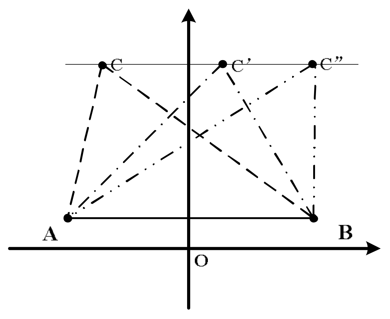
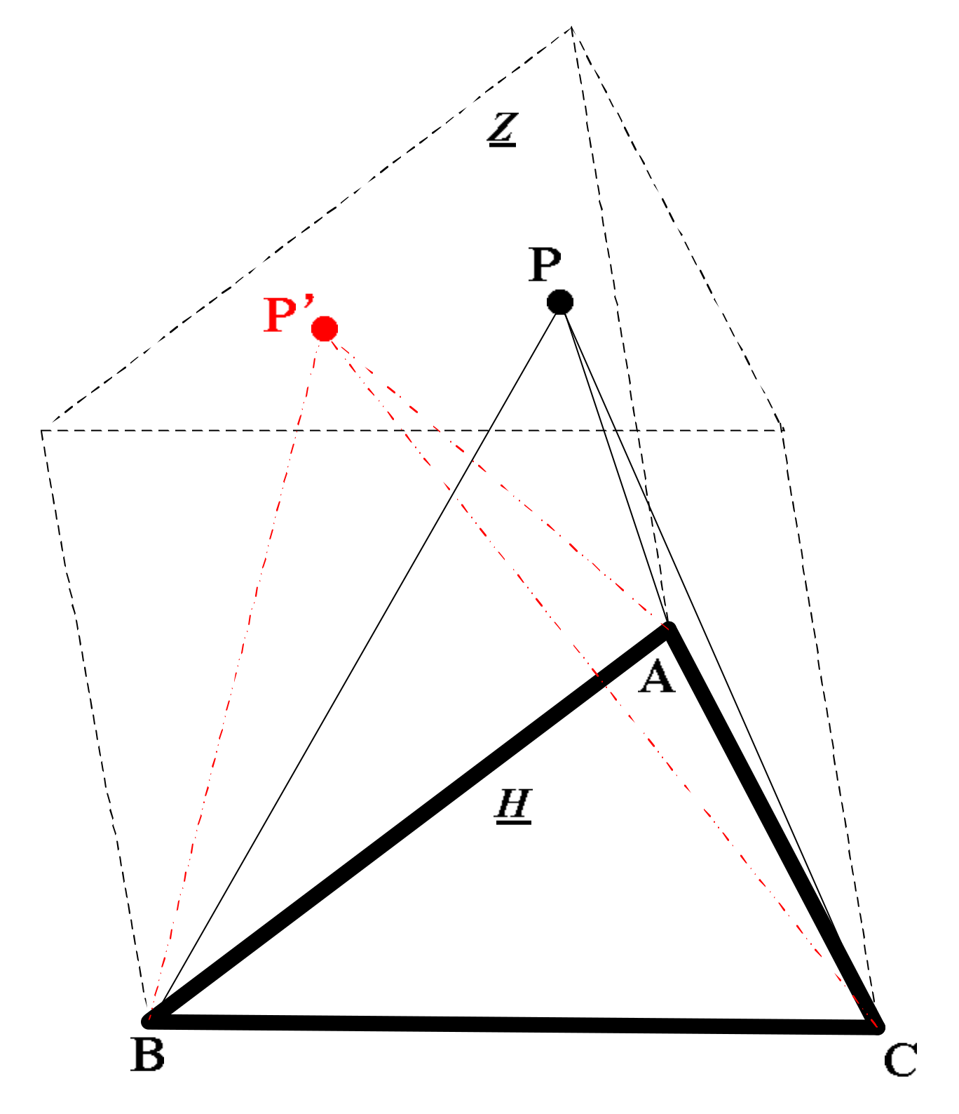
As we know, given a triangle with square area S, and an edge AB, the third point C is not unique. As in Figure 1, C’, C” and C can all meet this condition, because C’, C” and C are on the parallel line to AB. Actually, any point on this parallel line is feasible. Similarly, given a triangular pyramid of volume V, as shown in Figure 2, with the surface ABC fixed, the point P is not fixed. Any P’ on the parallel surface to ABC can be a suitable point P.
Meanwhile, inspired by non-negative matrix factorization, we introduce a proper constraint into the convex model and residual sum of squares (RSS) model. Non-negative matrix factorization has proved to be an effective method for automatically extracting endmembers and is able to find the most suitable pixel when no pure pixel exists [36]. However, the conventional solution of non-negative matrix factorization is not unique [33,34,51,52,53]. To alleviate this problem, a minimum volume constraint for the endmembers is introduced into the conventional NMF, which assumes that the endmembers are the vertices of the simplex in the feature space, as illustrated in Figure 1 and Figure 2. Given the same area of a triangle ABC and the two points, the third point is not unique. To make the solution unique, we can further impose a deviation constraint on the endmembers. It is a constraint based on the volume and the endmembers, which is computed by the endmembers and hyperspectral image. In summary, considering both volume and deviation, we can introduce a combination of the volume and deviation constraint into the NMF-based solution to endmember extraction.
In this paper, to adaptively determine the number of endmembers and automatically extract the endmembers’ spectra, a novel automatic sparse pruning endmember extraction method with a combined minimum volume and deviation constraint (SPEEVD) is proposed. Compared to the ICE and SPICE methods, the main advantages of SPEEVD for endmember extraction are as follows:
(1) The added term of the combination of the volume and deviation constraint by cross product in SPEEVD considers both the volume of the simplex and its deviation by cross product between endmember vectors. The cross product of endmembers in the hyperspectral dimension can not only clearly present the orthogonal direction between endmembers, but can also consider the volume of the simplex which is spanned by the endmembers. The cross product between vectors can eliminate some abnormal points and weaken the noise interference. Furthermore, the added term not only ensures the simplex’s minimum volume but also makes the simplex more compact.
(2) A sparse pruning method is proposed, which makes the proposed algorithm free from the limitation that the number of endmembers should be given. This roughly estimates the number of endmembers from the data itself, rather than a given initial value, whereas ICE needs an exact initial value and SPICE should use a large value. Our proposed method adaptively adjusts the endmember number to the real one, which makes it more practicable.
(3) The solution of matrix factorization is proposed to find an endmember and its corresponding abundance, which is actually a simplified solution of non-negative matrix factorization (NMF) [33,51,52], rather than the classical solution in ICE. This guarantees that the abundances of the endmembers are non-negative, with less computation cost.
The remainder of this paper is organized as follows. Section 2 reviews the ICE algorithm. Section 3 discusses the volume deviation using the cross product, and the sparse pruning terms in SPEEVD, and then presents the complete SPEEVD algorithm. Section 4 describes the experimental results with the simulated and real images. Section 5 provides the conclusions.
2. Review of the ICE Algorithm
The convex geometry model assumes that every pixel in an image is a linear combination of the endmembers of the scene. The convex geometry model can therefore be written as:
where i = 1, …, N. N is the number of pixels in the image, and M is the number of endmembers. is an additive perturbation (e.g., noise and modeling errors), is the kth endmember spectrum vector. is the endmember k’s corresponding abundance in the pixel i.
The abundances satisfy the constraints:
By minimizing the RSS, which is subject to the constraints in (2), the error between the real pixel spectra and the pixel constructed by the endmembers and the corresponding proportions from the ICE algorithm is minimized, i.e.,
The solution to the minimization problem for RSS is not unique. Therefore, a volume constraint is introduced, which is calculated by the sum of squared distances, i.e.,
As described in [40], ICE contains the RSS, and a volume constraint, so the objective function in ICE is:
where is the Frobenius norm, N is the number of pixels, and μ is the regularity parameter which balances the RSS error constraint and the volume constraint.
Combining (3) and (4), the objective function in ICE becomes:
With the objective function, each pixel in the image is processed iteratively to obtain the endmember E and the abundance P.
3. The SPEEVD Algorithm
This section describes the proposed sparse pruning endmember extraction algorithm with a combined minimum volume and deviation constraint (SPEEVD).
3.1. Volume and Deviation Constraint By Cross Product Between Vectors
The cross product in the hyperspectral dimension can not only clearly present the orthogonal direction between endmembers, but can also present the volume of the simplex which is spanned by the endmembers. We can therefore use the cross product to represent both the direction and volume scales, instead of the classical volume definition using only a scale determinant. In [54], a cross product between the 3-dimensional vectors and is defined as:
where , and are the unit vectors of the 3-dimensions.
Since the cross product in 3-dimensional space can be defined as in (7), the cross product generalizes into the (M + 1) dimension space, where d is given by:
while i1, …, iM+1 are the unit vectors of the (M + 1) dimension, and .
The direction of d is orthogonal to the hyperplane, which is spanned by , and the length of d is equal to the volume of parallelograms composed by the M vertices. The volume of the simplex V, composed of , is then defined as:
Therefore, according to (9), it can be inferred that:
while V is the volume of the simplex composed of .
We assume that are all of the desired endmembers from the image data, and that they span the space , while the undesired items such as noise or abnormal points are in the orthogonal subspace. As previously mentioned, the direction of d is orthogonal to the spanned hyperplane, so d is the normal of the hyperplane. The data is then projected to the direction d, which is similar to the direction of the orthogonal subspace of M. Therefore, the projected data is undesirable information, which should be minimized.
The deviation D, which can project data into the direction of d that is similar to the orthogonal subspace spanned by the endmembers, should also be minimized. It is defined as:
while is the data covariance matrix, and is the Frobenius norm of vector d.
Considering the combined constraint, the constraint is given as:
In (4), the volume constraint in ICE is calculated by the sum of squared distances, so (12) is inferred as:
The minimum volume constraint on the simplex spanned by the endmembers makes sure that the enclosing simplex is as small as possible, while the deviation constraint makes the vertices of the simplex more compact. Therefore, the combined constraint J′(E) takes advantage of the strengths of both individual constraints. Furthermore, the cross product between vectors is used to eliminate some abnormal points and reduce noise interference.
3.2. Sparse Pruning
A sparse estimate of p in [55,56] is defined as one in which irrelevant or redundant components are exactly zero, which is estimated by:
Therefore, the sparse constraint solution searches for the sparsest solution and ensures that the solution P has the smallest non-zero vector.
Considering the difference of the weights, the sparse constraint is given by:
where is the parameter which controls the sparsity. There are several ways of choosing . One possible way is to use a zero-mean Laplacian (rather than Gaussian) prior. According to [41,55,57], is given by:
Therefore, the sparse constraint (15) can be written as:
where T is the parameter which controls the sparse constraint. If the sum of a particular endmember’s proportion value is small, then the weight for that endmember becomes large. Therefore, this weight accelerates the minimization of these proportion values.
To apply the sparse constraint to abundances of unmixing, a sparse pruning without initial endmember number value is introduced. The initial number of endmembers is not required, in contrast with the other sparse promoting methods. We use singular value decomposition (SVD) to roughly estimate the number of endmembers from the data itself, then adaptively adjust the number of endmembers by the sparse pruning method. Since the initial roughly estimated number of endmembers M is larger than the true number of endmembers, the rank of the E matrix will not be full, and the corresponding abundance P matrix will be relatively sparse. A pruning method is then introduced to help the endmember E matrix adaptively prune until it cannot prune any more.
For each endmember signature, the maximum of the corresponding abundances of each pixel is computed, and it is judged whether they are under a threshold:
We can then prune the corresponding endmembers from the endmember set if their maximum abundance is under the defined threshold Tp.
Thus, our proposed method can self-adaptively adjust the endmembers by a sparse pruning in the unmixing procedure. With the sparse constraint on the abundances, which drives the abundance vectors of the corresponding endmembers that are unnecessary or non-existent in the image to be sparser, we get a relatively sparser abundance matrix. We then prune the endmembers from the endmember sets whose corresponding abundance vectors are under the threshold. Finally, we adaptively adjust the appropriate endmembers to represent the image.
3.3. SPEEVD
Based on the above analysis, an automatic sparse pruning endmember extraction with a combined minimum volume and deviation constraint (SPEEVD) algorithm is proposed. Like ICE, SPEEVD is also based on a convex model, with the common assumption about the errors in models and the appropriate statistical procedures. A simplex volume can contain most of the data point set while excluding the abnormal pixels out of the minimum simplex. The other added term is sparse pruning, which can automatically prune those endmembers that are under the threshold.
3.3.1. Problem Formulation
Based on the RSS model and the convex model, and consisting of a combination of the constraint on deviation of volume (13) and the sparse constraint on abundance (17), the objective function is defined as:
where X is the image data, N is the number of pixels, E and P are the endmember matrix and corresponding abundance, is the Frobenius norm, and μ and λ are the two regularization parameters which balance the RSS error, volume of endmembers and the sparse constraint on the abundances.
The first part in (20) is the RSS term, which is the same as in ICE. The second and third parts are what we introduced in the previous section. Substituting (3) and (17) into (20) we get:
where pik is the proportion of endmember k in pixel i, is the k endmember spectral set, and T is the parameter used to control the sparse pruning process.
The added term about volume and deviation J’(E) in (13) can be combined with (10), and (13) can be calculated as:
The endmember volume V is affected by the sum of the squared distances, which can also be calculated as:
Therefore, considering (23), (22) can be expressed as:
Since in (21), the objective function about P is convex, convex optimal algorithms can be used to solve P. However, considering the added E constraint, J’(E), the objective function about E is not convex, so we cannot use a convex optimal method to solve E. To simplify the solution, V is estimated by k iterations, while D in (22) is calculated by endmembers in the previous k − 1 iterations, so the J’(E) about E is convex.
The added term G(P) in (21) imposes the sparse constraint on the abundance; meanwhile, the sparse pruning endmember method is also included in the processing. The sparse pruning endmember method first adds the sparse constraint, which drives the abundance vectors of the corresponding endmembers that are unnecessary or non-existent in the image to be sparser. It then prunes endmembers from the endmember sets whose corresponding abundance vectors are under the threshold. Thus, it can adaptively adjust the number of endmembers.
3.3.2. Pre-Processing and Initialization
Like many other endmember generation methods, our method also first needs a dimensionality reduction procedure. In our method, a minimum noise fraction (MNF) transform is employed to reduce the data.
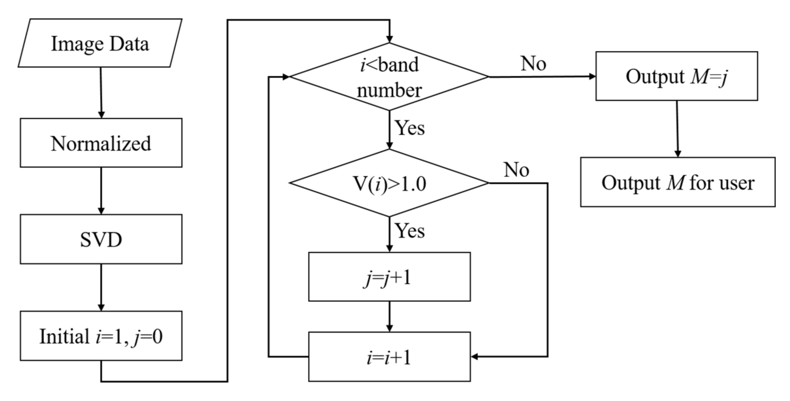
In this paper, the initialization of the number of endmembers is roughly estimated from the data itself, as shown in Figure 3, rather than a subjectively given value. SPEEVD estimates the number of endmembers from the data itself, so that it decreases the need for one parameter, while the number of endmembers in SPICE should be strictly defined as a number larger than the true endmember number. This may be difficult for the user without enough knowledge. The initial M in SPICE is given by the user, whereas in the proposed SPEEVD method the initial M value is not given by the user but is determined by calculating what number of SVD eigenvalue can meet the condition that the eigenvalue is above the empirical threshold, as in the method described in [40]. This is the primary difference between the proposed SPEEVD and SPICE.
The following flowchart in Figure 3 demonstrates how to determine the initial M in SPEEVD. The SVD of the data is first executed, and the eigenvalues above the threshold are kept. Here the threshold is 1.0, for the eigenvalues above 1.0 contain the signal information [40]. The number of the remaining eigenvalues is then recorded as M. The M chosen bands of the MNF bands are used as observation data for the following process, and the initial number of endmembers is set as M.
Initialize the endmember matrix E, abundance P. Set the maximum iteration number Tm, the tolerance of the objective function Te, and the regularization parameters μ, λ and T.
3.3.3. Optimization Algorithm Description
To minimize the objective function in (21) with respect to both P and E is actually a combinatorial optimization problem. This technique treats the original optimization problems as two sub-problems, with the following iterative update rule:
To solve P and E in (25), a simplified alternative projected gradient descent method is used. To solve P, the projected gradient learning method with non-negative constraint can be used as:
where the parameters are the small learning step sizes selected based on the Armijo rule [36]. Equation (26) can ensure that the abundance is physically significant (e.g., P ≥ 0), and that the abundance is non-negative in the iterative procedure.
Similarly, E can be determined through the gradient descent method, as in (26). Taking the solution of E as (26), the solution of P and E can be regarded as a kind of alternative non-negative solution, which is a little time consuming. However, the E matrix can be solved explicitly in (26) with a given P. As previously mentioned, J’(E) is calculated by D and V in (24). To save computation cost, the scale of D can be calculated by the k − 1 iteration of endmember E, while V is estimated by the k iterations with the endmember matrix. Therefore, in the k iteration, the objective function about E is still convex. Therefore, a quadratic program can be used to solve E.
Taking the partial derivative of (21) with respect to E, we get:
We then minimize the objective function in (21) with the previously obtained P matrix, so the endmember ej can be solved by:
where x is the pixel reflectance in the image, IM is the M ∗ M identify matrix, and 1 is the vector of ones. As previously mentioned, the scale of D is calculated by the previous iteration of E.
In the sparse pruning process, the endmembers are adaptively pruned through the given threshold of the abundances. Once the abundance of one endmember is under the threshold, it deletes the corresponding endmember from the endmember matrix so that it can adaptively prune to the true number.
3.3.4. Stopping Criterions
In SPEEVD, the iteration procedure stops when the ratio of successive values of the objective function is less than the tolerance, or when the number of iterations reaches the prescribed maximum number. To avoid being trapped in local minima, some increasing steps of the objective function are allowed in the search procedure. If the successive increasing steps are over a predefined value, it will break the loop.
The proposed SPEEVD algorithm (Algorithm 1) is summarized as follows:
| Algorithm 1: The procedure of the SPEEVD framework. |
| Input: hyperspectral image data |
| (1) Pre-processing: Use the first M bands data after MNF transformation as observation data, where the value of M is obtained according to Figure 3. (2) Initialization: k = 0. Choose the regularization parameter , parameter T, threshold Tr, endmember matrix E. (3) Compute D using the formulation (11), and combine with E, using a quadratic program to solve P. Update , while k←k + 1 (4) Then, with the latest P, renew in the E set by the formulation (28). Prune the endmember vector from the E matrix whose corresponding abundance is below the threshold Tp, as Equation (19): , where D is a scale, using the latest iteration results of E to compute by , ensuring that E is non-negative, which is physically significant. Update While k←k + 1 (5) Repeat this cycle (3)–(4) until the stopping criterion is satisfied. (6) Execute inverse MNF transform to E, obtain Ê. |
| Output: endmember matrix Ê and abundance matrix P. |
4. Experiments and Analysis
In this section, the proposed SPEEVD algorithm is applied to a series of simulated images and the well-known Cuprite AVIRIS data in a MATLAB environment. A simulated image is used since all its endmembers are known in advance, so it is easy to manipulate the parameters and undertake a quantitative analysis. SPEEVD is compared to VCA [25], N-FINDR [24], SGA [26], C-NMF [34], MVC-NMF [36], ICE [40], and SPICE [41], which are all based on the convex model.
VCA is an endmember extraction algorithm, which repeatedly performs orthogonal subspace projections resulting from a sequence of gradual growing simplexes vertex by vertex to find new vertices. The N-FINDR is an automated approach that looks for the set of pixels which define the simplex with the maximum volume, potentially inscribed within the dataset. Simplex growing algorithm (SGA), is a sequential algorithm to find endmember, which sequentially finds a simplex with the maximum volume every time a new vertex is added. C-NMF extract endmember based on nonnegative matrix factorization with piecewise smooth and sparse constraint. MVC-NMF extract endmember based on nonnegative matrix factorization with the minimum volume constraint. ICE combines the convex geometry model with suitable assumptions about errors in the model and appropriate statistical procedure to extract endmember. SPICE is an extension of ICE, which combines the convex geometry model with sparse promoting priors.
4.1. Experiment with Simulated Images
Simulated images of 100 × 100 pixels and 224 spectral bands are synthesized with five signatures randomly selected from the USGS library, and their corresponding fraction abundances, which are non-negative and generated by Dirichlet distribution, and are submitted to a sum-to-one constraint. The five chosen spectra are resampled to correspond to the AVIRIS data. The five signatures from the USGS library are Carnallite_HS430.3B, Chlorite_HS179.3B, Clinochlore_NMNH83369, Clintonite_NMNH126553, and Corundum_HS283.3B.
The experiments are classified into four groups. In the first group, we investigate the performance of SPEEVD compared to the other previously mentioned methods. In the second group, we study the robustness regarding noise interference. The third experiment aims at comparing the performances for data without pure pixels, with various degrees of mixing. The mixing degree is denoted by purity, which equals the highest abundance value of the whole abundance matrix. The fourth experiment tests different initial parameters.
4.1.1. Experiment 1
In this experiment, the image size is fixed at 100 × 100, the purity is fixed at 0.7, and the signal-to-noise ratio (SNR) is fixed at 45. The experiment is intended to test the robustness of SPEEVD compared to the other state-of-the-art methods.
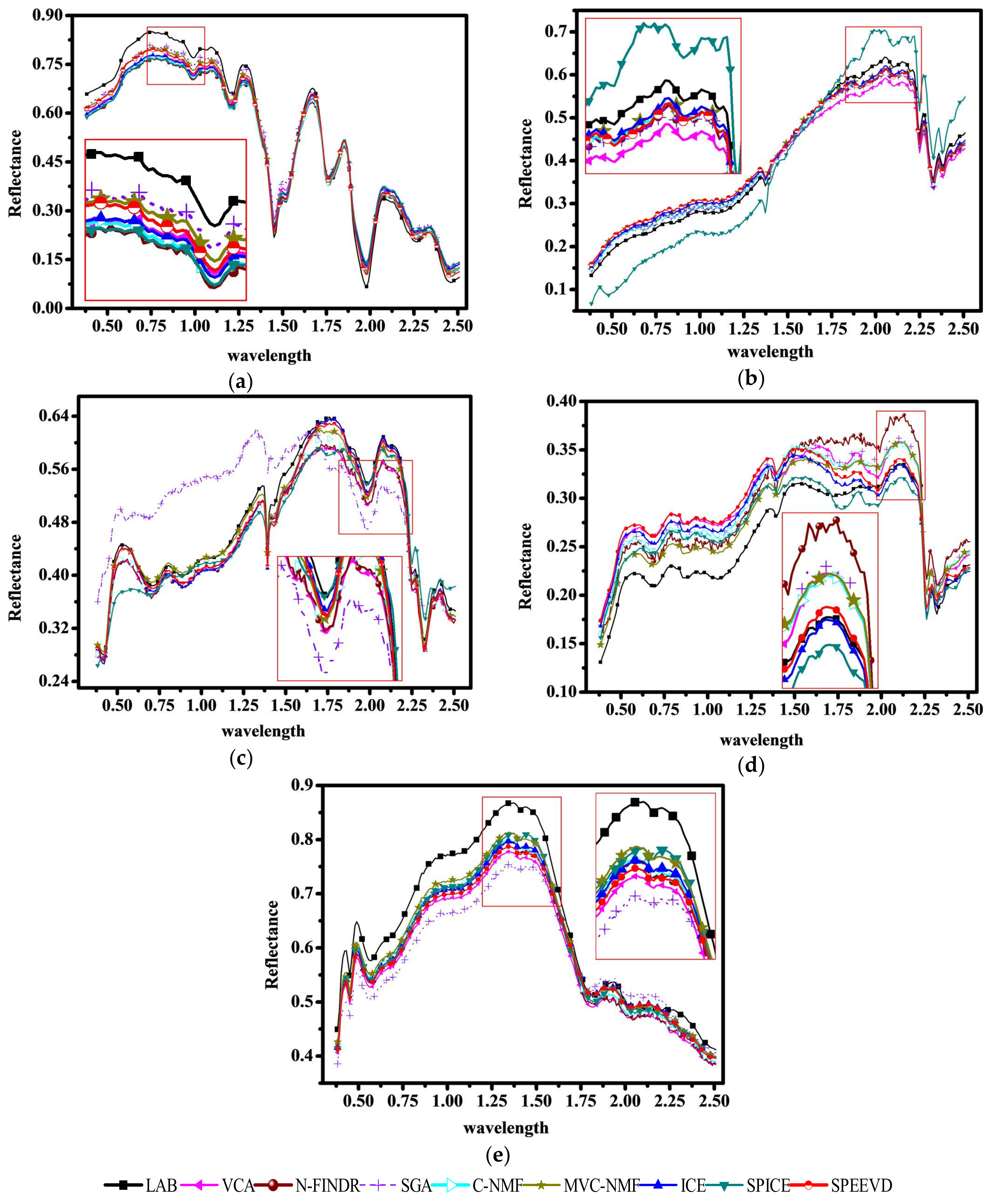
The spectra generated by the five endmember extraction methods are shown in Figure 4, where the spectra in the small red rectangle is enlarged separately for each figure. The correlation coefficient metric and spectral angle distance are used to compare the similarity between each extracted endmember spectra and the corresponding library reference spectra.
To quantitatively assess the performance of the different endmember extraction methods, we use the correlation coefficients, the cosine of the SAD metric, and the SID-SAD metric.
The classical correlation coefficient metric between pixel a and b is defined by:
where is the covariance matrix between and , and and are the deviations of and , respectively. The well-known SAD metric between pixel a and b is given by:
where and are the norms of and , respectively. The SID-SAD metric in [35] between pixel a and b is given by:
The correlation coefficients, cosine of the SAD metric, and the SID-SAD metric are used to compare the similarity between each extracted endmember spectra and the reference spectra. The correlation coefficients between the reference spectra and the extracted spectra with VCA, N-FINDR, SGA, C-NMF, MVC-NMF, ICE, SPICE, and SPEEVD are shown in Table 1. The more the similarity, the larger the correlation is. With the cosine of SAD in Table 2, a larger cosine of SAD suggests a larger similarity. Finally, in Table 3, the more the similarity is, the less SID-SAD (*10 − 5) is.
The correlation coefficients in Table 1, the cosine of SAD values in Table 2, and the SAD-SID metric values in Table 3 all show that the five endmembers’ spectra by SPEEVD are more similar to the library spectra, compared to VCA, N-FINDR, SGA, ICE, and SPICE. Once given an accurate initial number and proper parameters, C-NMF and MVC-NMF obtain a promising result; however, SPEEVD obtains satisfactory results even without initial values of numbers. Since there are no pure pixels in the simulated image, VCA, N-FINDR, and SGA, which are endmember search algorithms, obtain worse results than the other endmember generation algorithms. SPEEVD considers the volume by cross product and its deviation, rather than the volume, which ensures that the simplex is the minimum volume, and makes the points of the vertices closer in the scattered feature space.
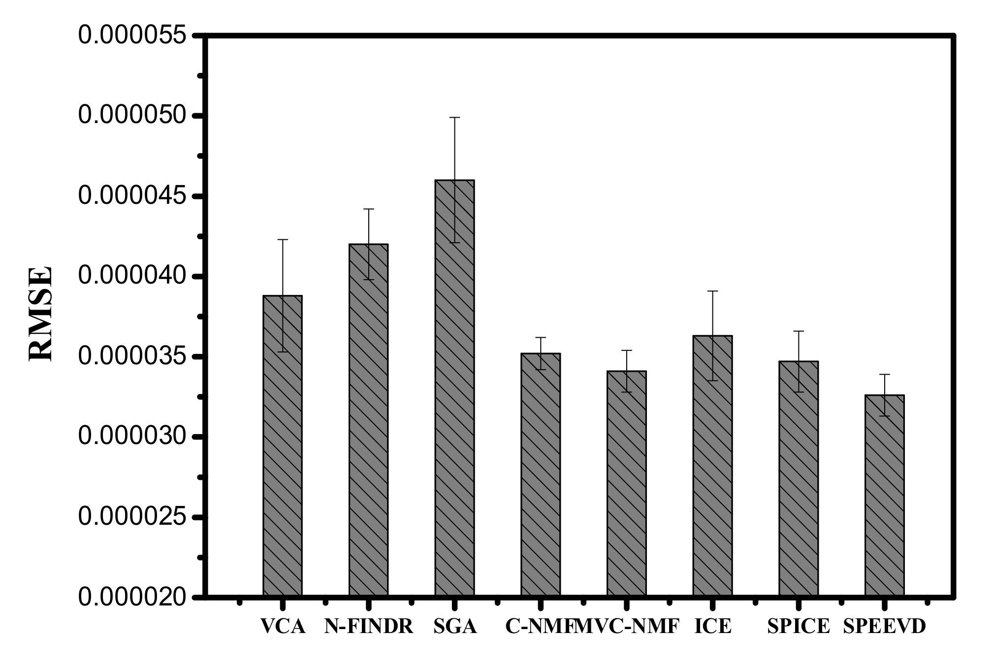
Figure 5 shows the RMSEs after reconstructing the simulated image using the endmembers extracted by the different methods. The RMSEs in Figure 5 show that SPEEVD gives better results than the other methods, because it can shrink to the proper endmember number, and keeps the accuracy of the extracted endmembers. The RMSEs of VCA, N-FINDR, and SGA are higher than the other methods, which verifies that the basic assumption of these methods fails in the simulated image. With proper parameters, MVC-NMF obtains better results than ICE and SPICE. However, SPEEVD is free from the initial value of endmember number restriction, whereas SPICE still needs a large, rough initial number.
4.1.2. Experiment 2
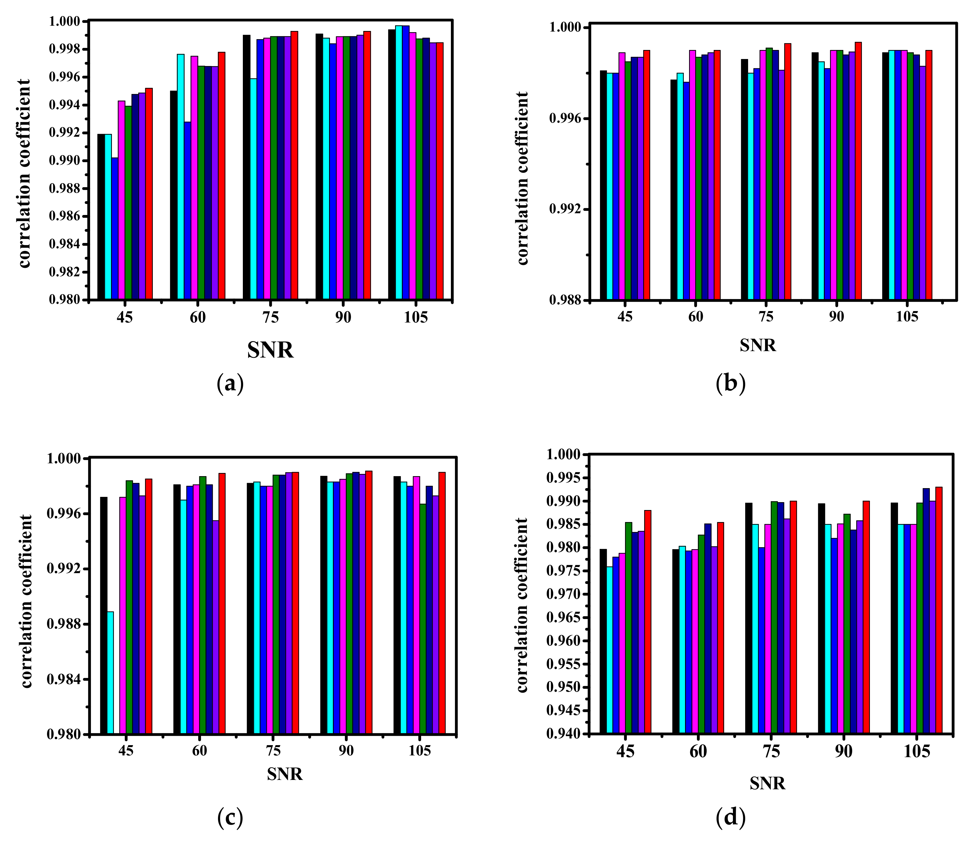
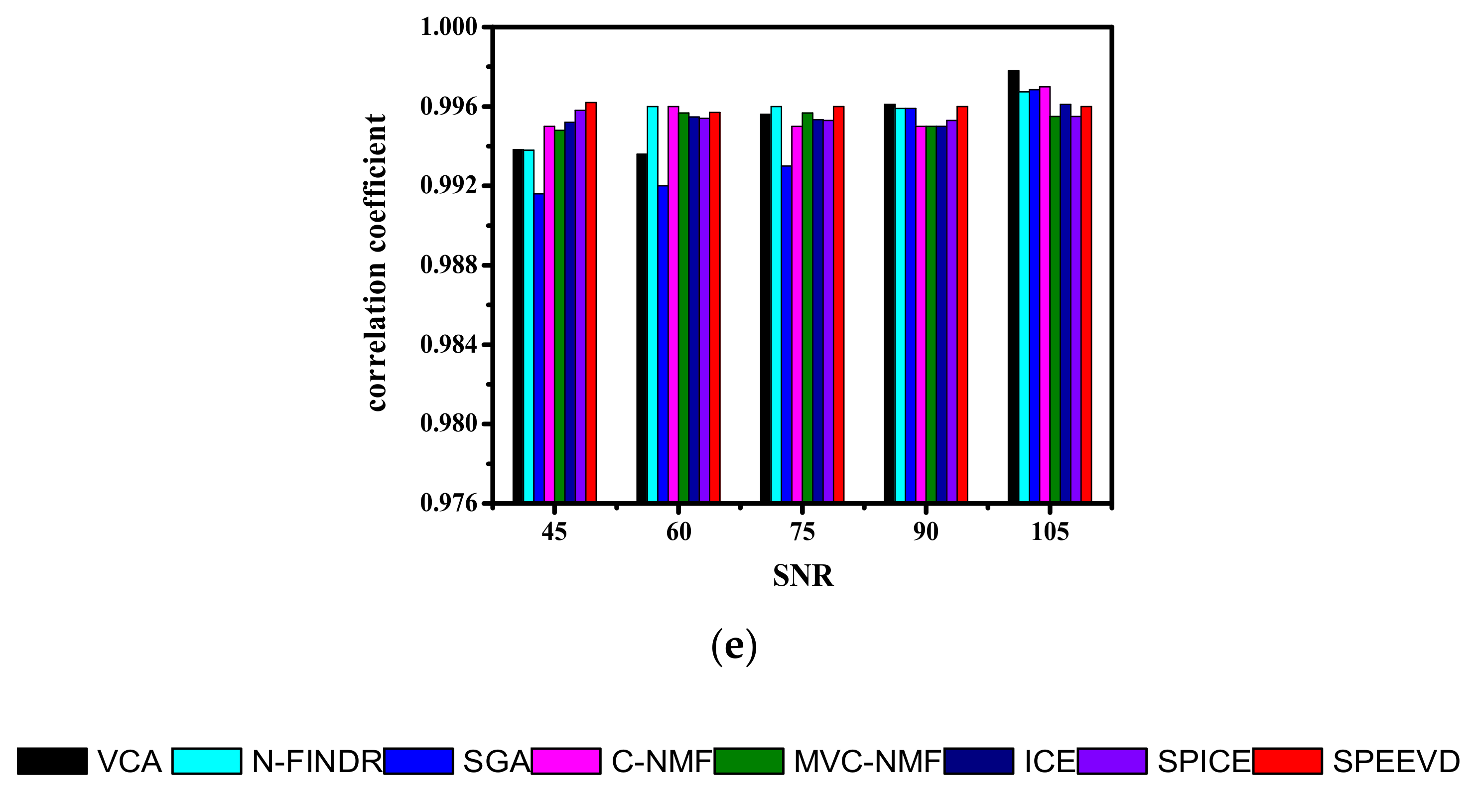
In this experiment, SNR is varied from 45 dB to 105 dB. The image size is 100 × 100 and the purity is fixed at 0.85. The experiment is intended to test the robustness of SPEEVD regarding noise interference.
As the SNR increases, the performances of the methods in Figure 6 are measured through the correlation coefficients between the methods and the library reference spectra. The higher the correlation coefficients value is, the more similar the extracted spectra and library spectra are. The experimental results show that their performance becomes better as SNR increases especially in Figure 6a,b. Overall, SPEEVD shows better results than the other methods. Four of the five endmembers with SPEEVD method present the largest values in Figure 6. However, even with lower SNR, MVC-NMF, ICE, SPICE, and SPEEVD still give reliable results.
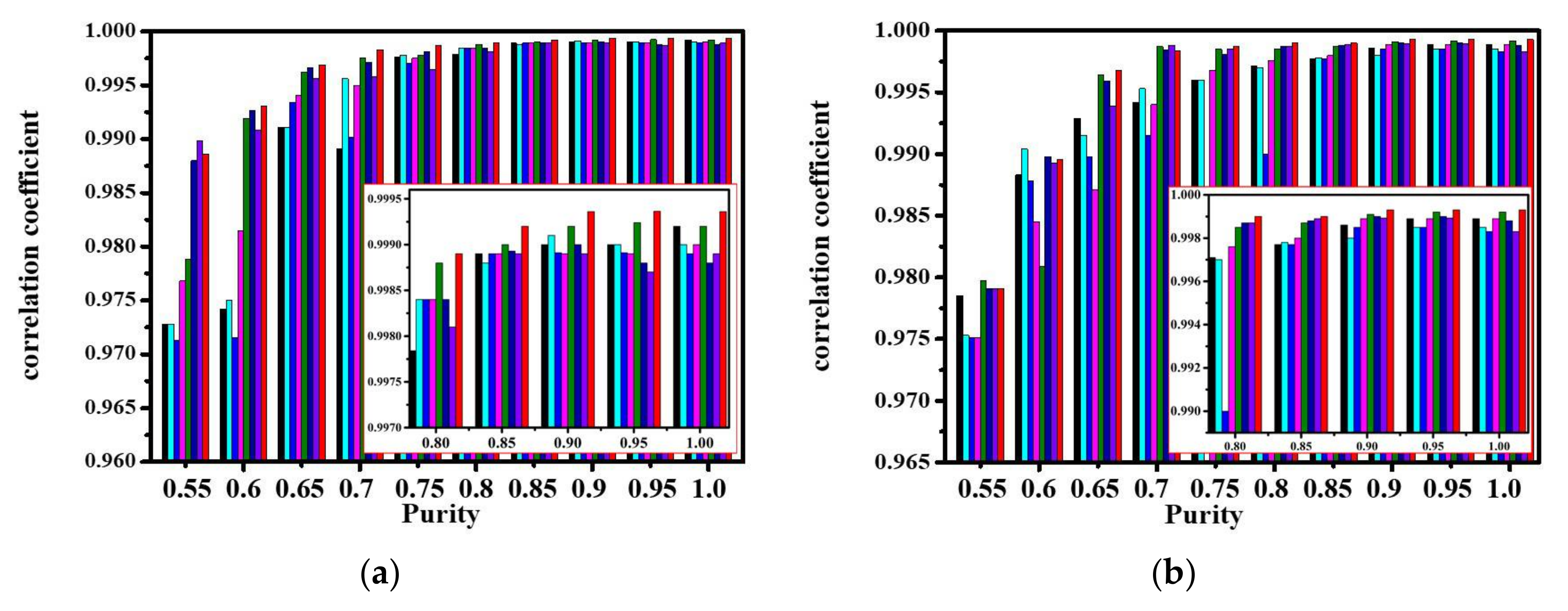
4.1.3. Experiment 3
In this experiment, the degree of mixing is denoted by purity, which equals the highest abundance value in the whole abundance matrix. The purity is varied from 0.5 to 1.0 in this experiment. The image size is 100 × 100 and the SNR level is fixed at 105 dB. The third experiment aims to compare the performance for data without pure pixels, with various degrees of mixing. To show clearly the differences between methods, the purity values from 0.8 to 1.0 are enlarged, as shown in the red rectangle of each figure.
As the purity increases, the performance of the methods is measured through the correlation coefficients between the methods and the library spectra, as presented in Figure 7. At lower purity, all the methods obtain poor results. However, as the purity increases, the performances improve; in particular, VCA increases relatively quickly. As the purity reaches 0.85, the performances reach convergence. However, at a purity of 0.65 in Figure 7d, each of the methods presents bad results. It is possible that the maximum purity of the whole image dataset is 0.65, while the maximum purity of Clintonite may be far below 0.65. If the maximum purity of Clintonite is far below 0.65, it suggests that the spectral contribution of the Clintonite endmember to the mixed pixel is concealed by the other four endmembers.
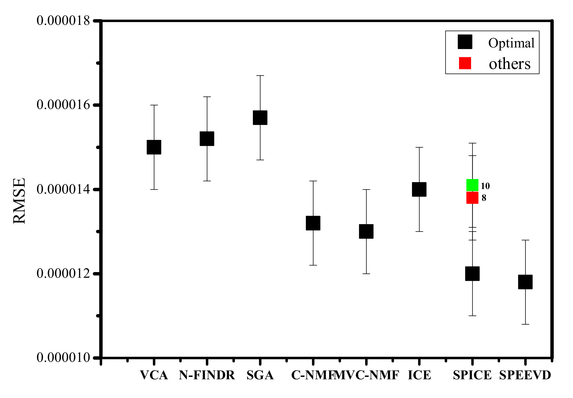
4.1.4. Experiment 4
In this experiment, the effect of the initial number of endmembers is investigated. VCA, N-FINDR, SGA, C-NMF, MVC-NMF, ICE, SPICE, and SPEEVD are compared. VCA, N-FINDR, SGA, C-NMF, MVC-NMF, and ICE need predetermined VD, the initial numbers of which are set to five, the real dimensionality. The initial number is not needed in SPEEVD, while it is required in SPICE. The initial values for SPICE are set to 10, 8 and 6 (in Figure 8 the result of 6 is black, 8 is red, 10 is green), respectively. With proper parameters, both the SPICE and SPEEVD results can prune to the true number of five.
Figure 8 shows that with a larger estimated number, SPICE and SPEEVD obtain a lower RMSE of unmixing. However, C-NMF, ICE, MVC-NMF, SPICE, and SPEEVD show better results than VCA, N-FINDR, and SGA.
Experiment 5: In this experiment, the effect of the parameters on the initial endmember number M in SPEEVD is investigated.
As µ and T are regularized parameters in the objective function (21), several pairs of parameters are used to execute the experiment, and the following representative results are shown in Table 4.
With all the above different parameters, the estimated number of endmembers is still five, which reveals that SPEEVD can prune to the true number with different parameters.
4.2. Experiments with Cuprite Image AVIRIS Data
A 190 × 250 sub-image of Airborne Visible/Infrared Imaging Spectrometer (AVIRIS) hyperspectral image data covering Cuprite, Nevada (Figure 9a), is tested with VCA, N-FINDR, SGA, C-NMF, MVC-NMF, ICE, SPICE, and the SPEEVD algorithm. The spatial and spectral resolutions of the images are 20 m and 10 nm, respectively, with 224 spectral bands between 0.4 and 2.4 μm. After water vapor absorption bands near 1.4 and 1.9 μm, and low-SNR bands are removed, 182 bands of the sub-image are used for the experiments.
In this part, we carry out the first experiment to study the performance of SPEEVD, compared to VCA, N-FINDR, SGA, C-NMF, MVC-NMF, ICE, and SPICE. VCA, N-FINDR, SGA, C-NMF, MVC-NMF, and ICE need an accurate estimated VD, while SPICE just needs an initial value, which does not need to be exact. The VD is estimated to be approximately 10 using the HySime test and NWHFC test with Pf = 10 − 5 and the reference map [58]. We infer that there are 10 minerals included in the sub-image; therefore, the initial number of endmembers for VCA, N-FINDR, SGA, C-NMF, MVC-NMF, and ICE is set to 10. For SPICE, the initial number of endmembers is set to 15. In the second experiment, the key parameter μ in SPEEVD is investigated.
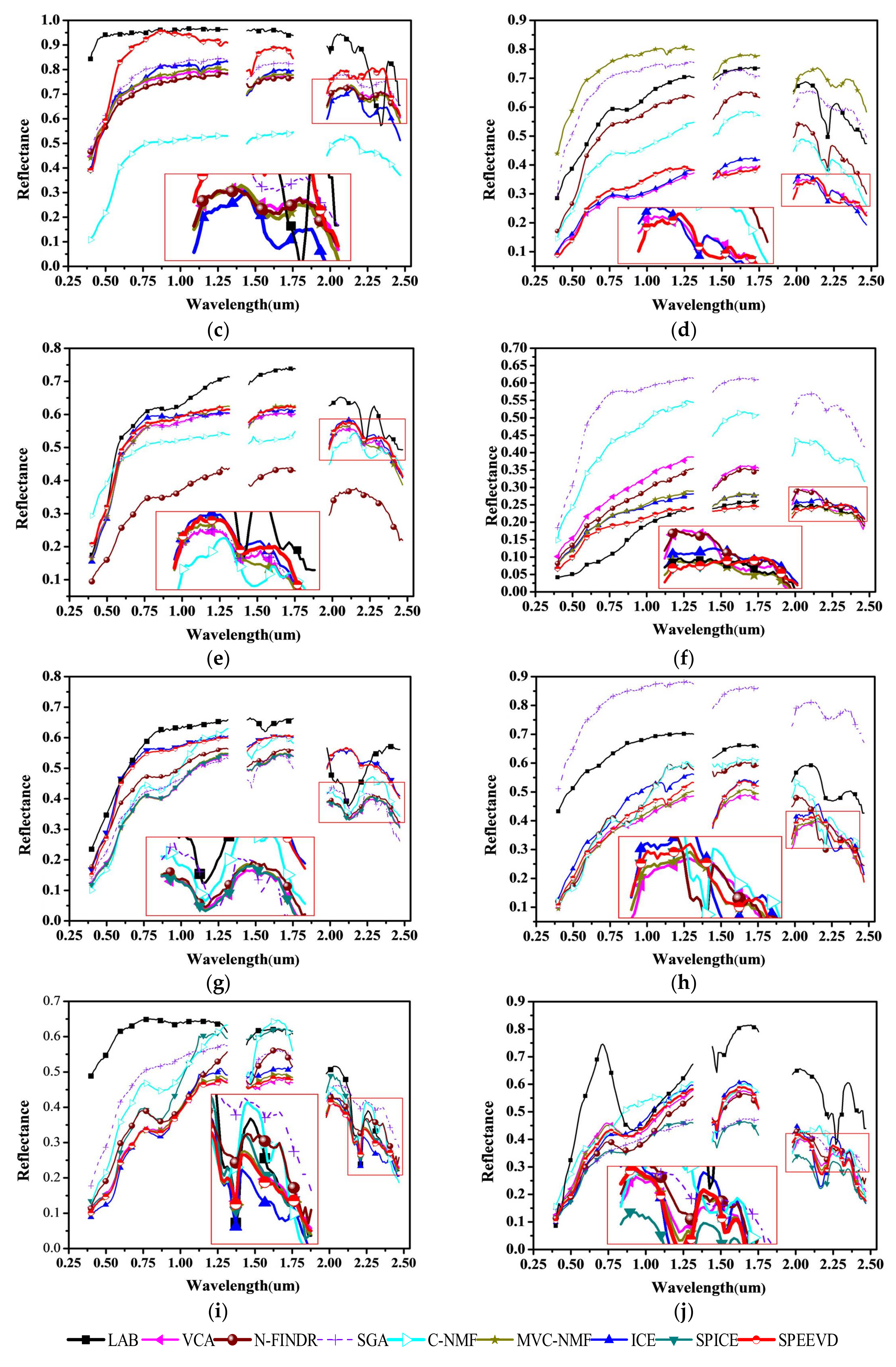
According to published papers, and the reference map [58], this well-known AVIRIS image contains minerals including calcite, alunite, sphene, kaolinite, montmorillonite, buddingtonite, chalcedony, muscovite, jarosite, and desert varnish. In [58], kaolinite, alunite, chalcedony, and desert vanish prevail in the sub-image. Since there are unknown true endmember spectra, the USGS library spectra are used as reference, as in many other published papers [24,25,59]. The extracted spectra of alunite, kaolinite, and montmorillonite, by the previously mentioned methods, are similar to the USGS library spectra. The extracted spectra of jarosite is, however, a little different from the USGS library spectra. The according abundance of jarosite is very low and is mixed with alunite, which may be one of the reasons for this phenomenon.
Given the proper parameters, SPICE and SPEEVD can adaptively obtain ten endmembers. Therefore, the results with ten endmembers are compared to the other previously mentioned methods. By a side-by-side visual comparison of the extracted endmember spectra with the various methods in Figure 10, where the endmember spectra in the small red rectangle is enlarged separately for each figure, we observe that they generally identify similar minerals. However, VCA and ICE show a difference in Figure 10g. As there are no pure pixels in the image of Figure 9, the assumption of VCA may not be satisfied; thus, the results with VCA are the worst. ICE does not consider the sparsity of abundances, so that the extracted chalcedony’s spectra by ICE is a little different from that of the others.
To quantitatively investigate the performances of the endmember extraction algorithms, the correlation coefficients, the cosine of the SAD metric, and the SID-SAD metric are used. The experimental results are listed in Table 5 (correlation coefficients), Table 6 (cosine of SAD), and Table 7 (SID-SAD), respectively.
In the above tables, SPEEVD shows better results than VCA, N-FINDR, and SGA. As no pure pixels exist in the sub-image, the basic assumption of VCA and SGA is not satisfied, so VCA and SGA get worse results. The SPEEVD algorithm is free from the constraint that pure pixels should exist in the sub-image, and it generates an endmember matrix instead of searching for endmembers within the sub-image. SPEEVD therefore gives better results than VCA. In Table 5, the average correlation coefficient for SPICE is better than for MVC-NMF, whereas in Table 6 the cosine of the average spectral angle distance for MVC-NMF is better than for SPICE. In Table 7, the SID-SAD metric values for C-NMF, MVC-NMF, ICE, SPICE, and SPEEVD are better than for VCA, N-FINDR, and SGA, with the SPEEVD results being the best among all the methods. The constraint of SPEEVD considers both the volume and its deviation, rather than only the volume of the simplex composed of endmembers. This ensures that the simplex is compact and makes the points of the vertices closer in the scattered space, eliminating some abnormal points.
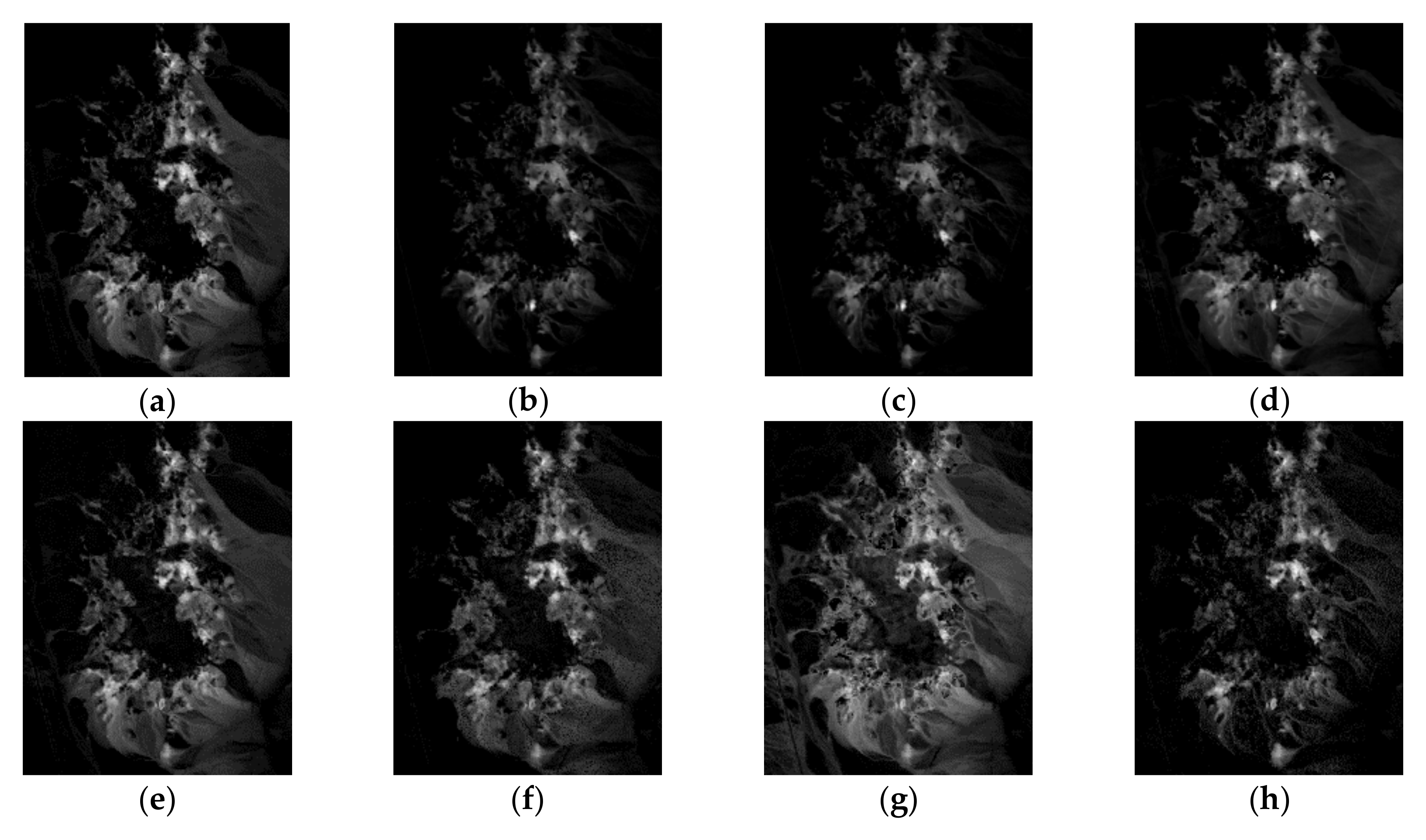
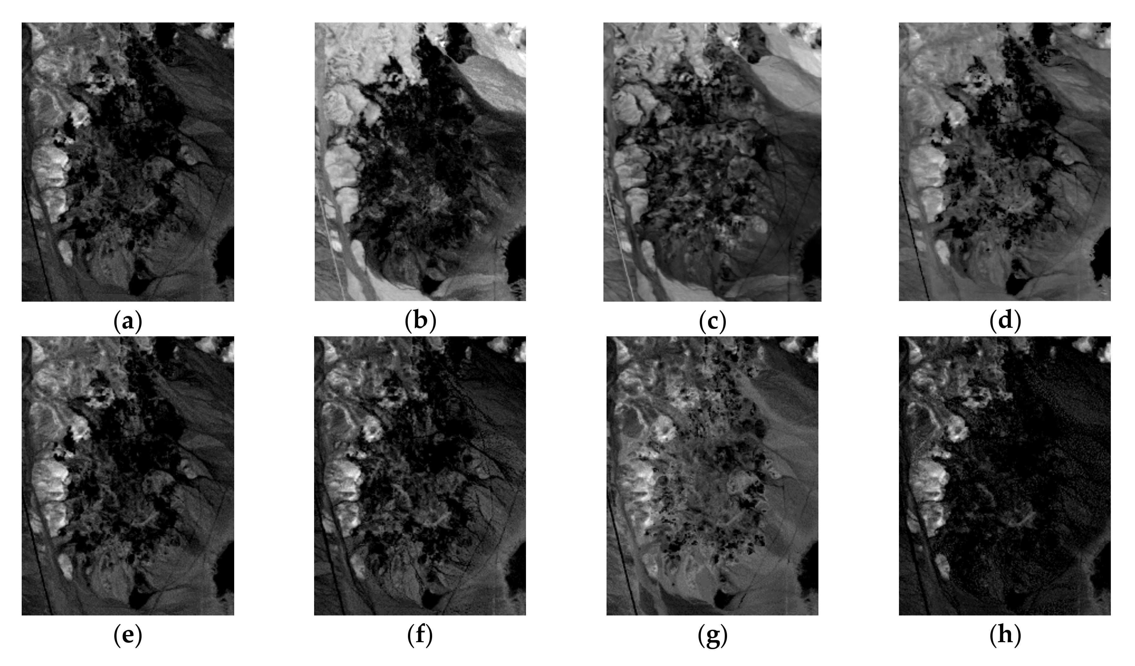
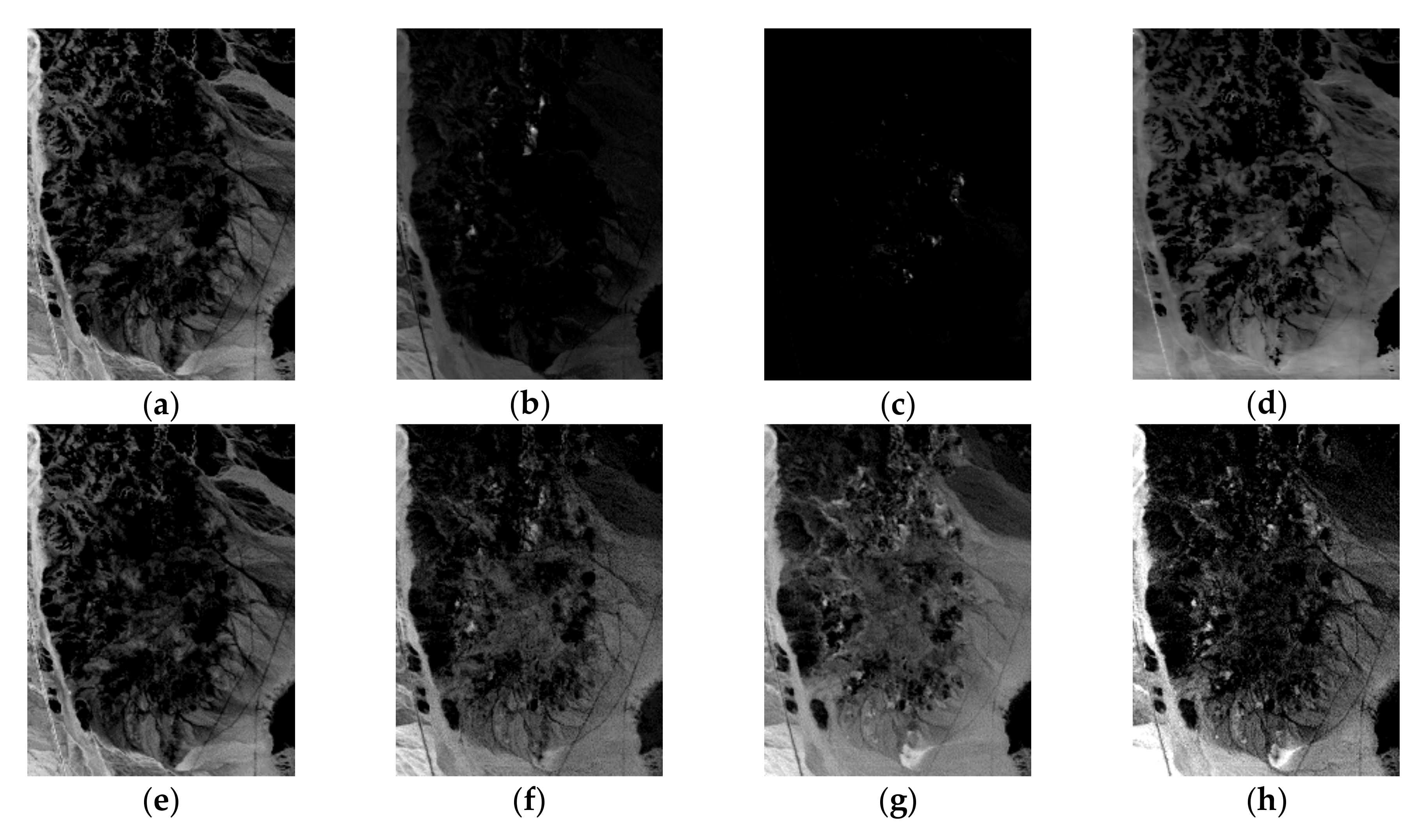
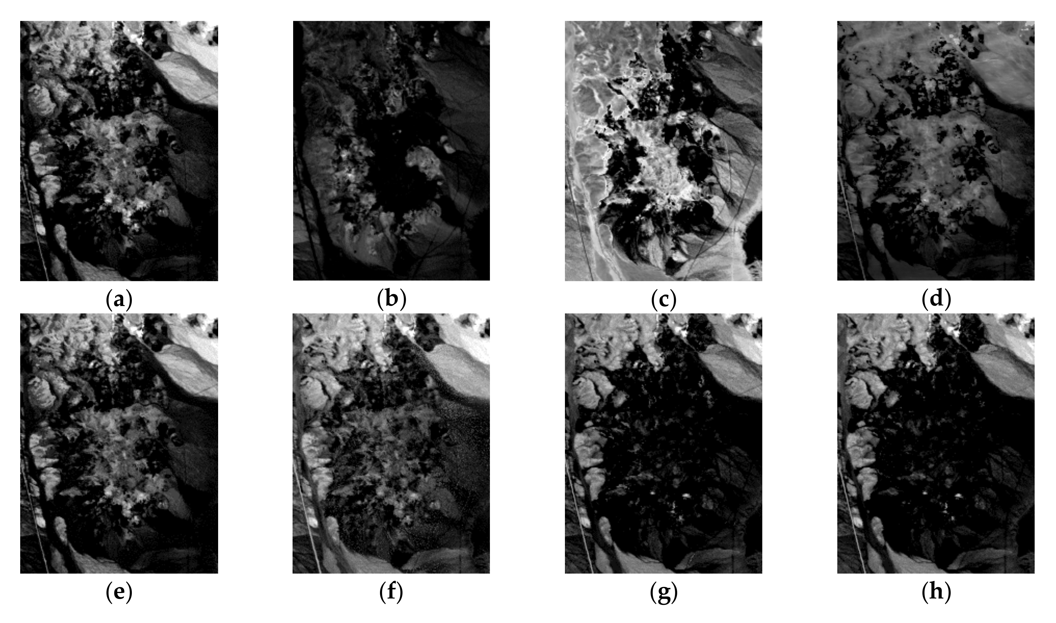
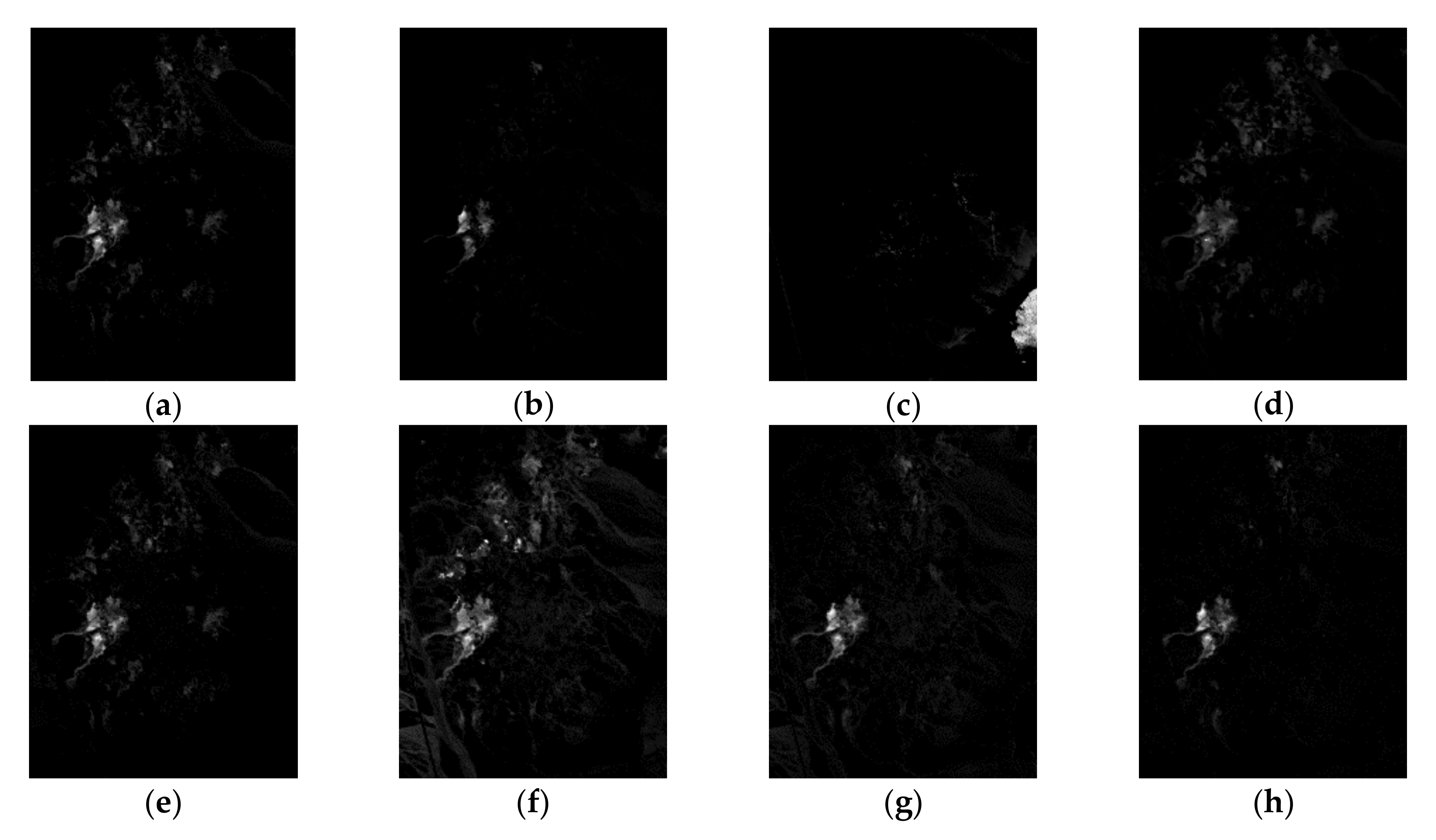
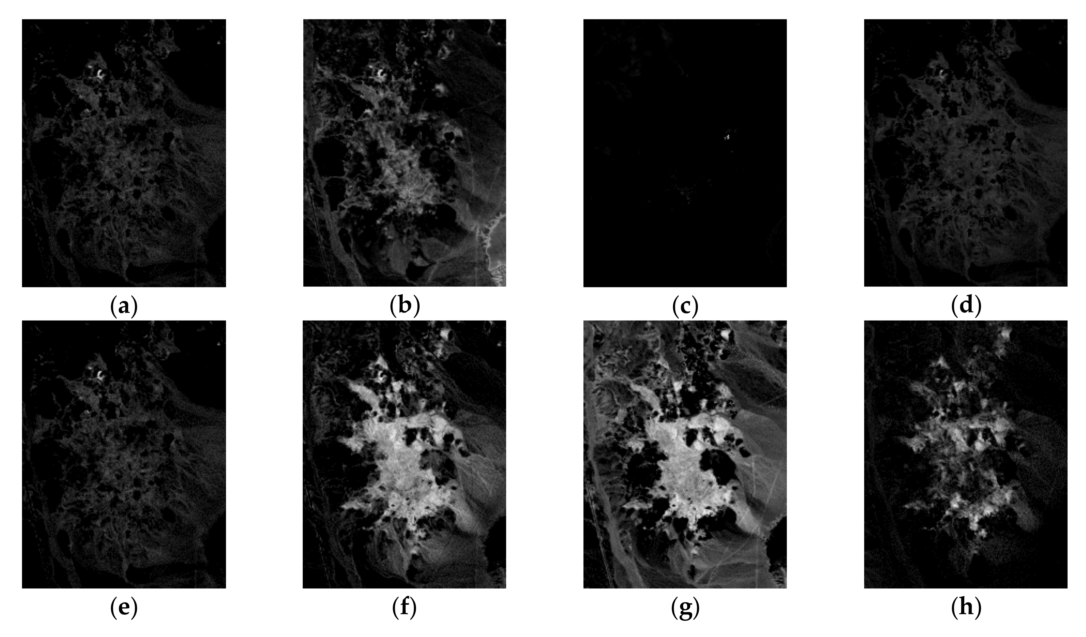
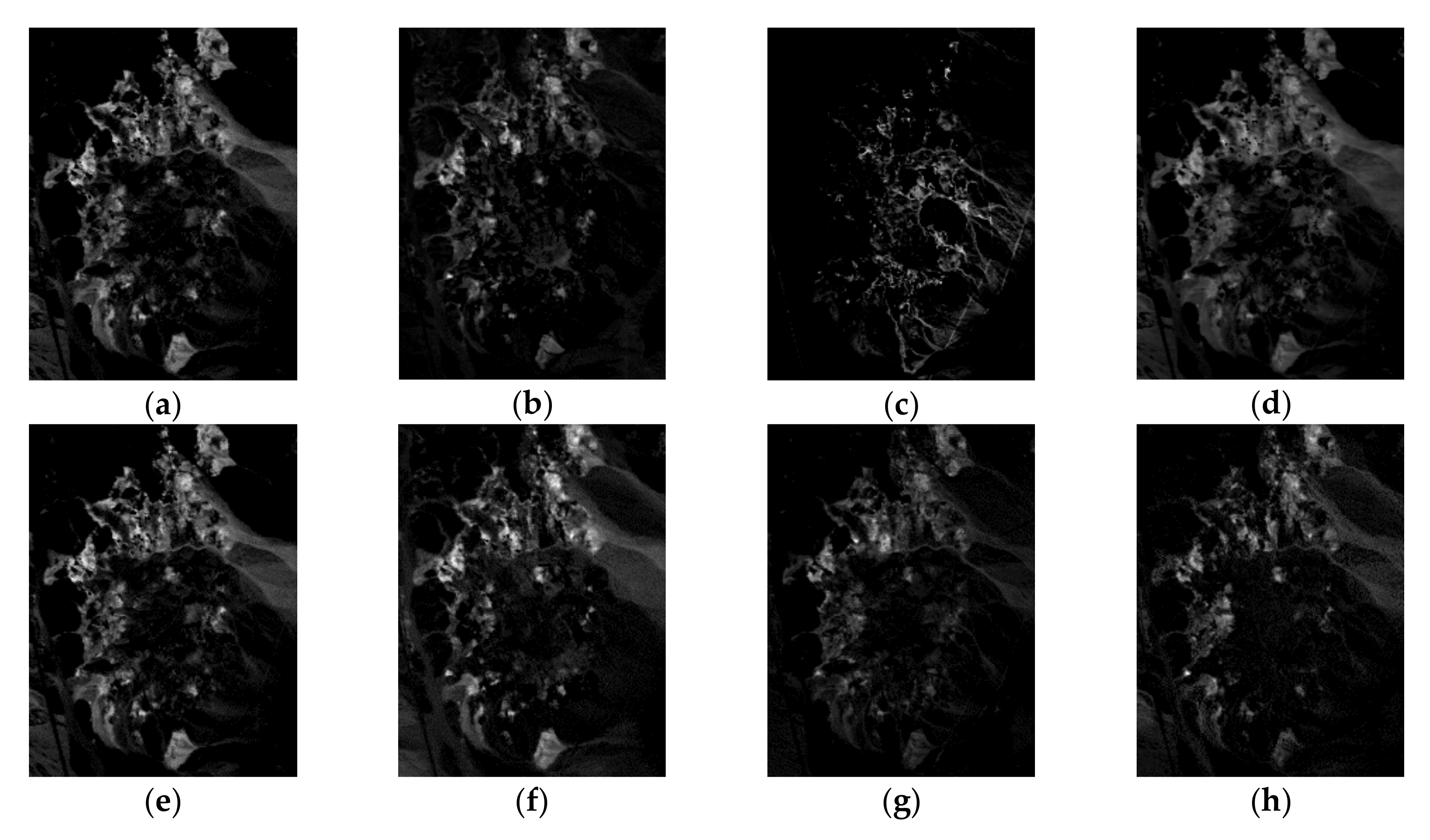
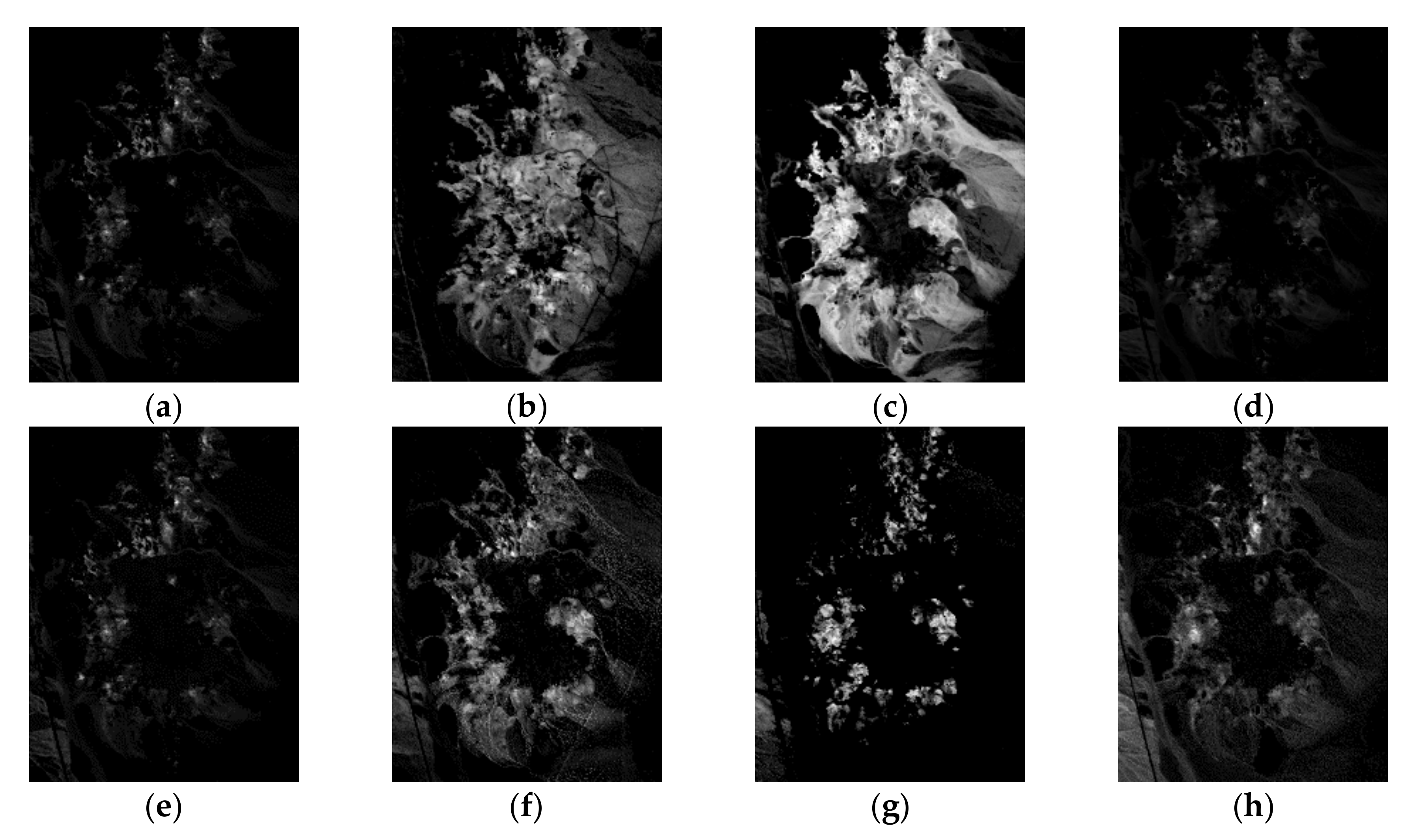
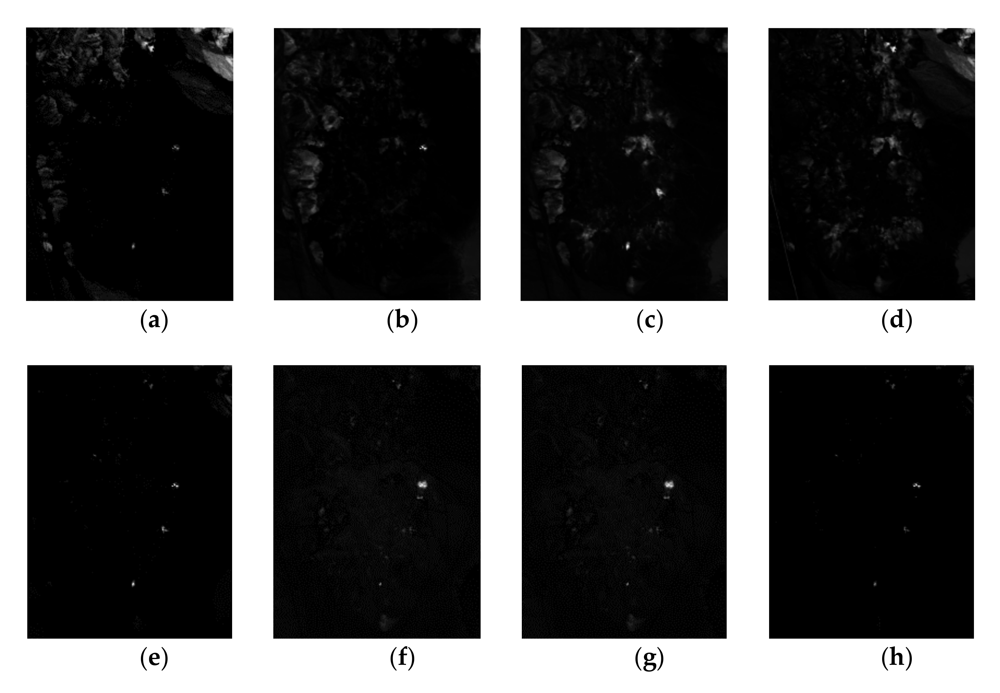
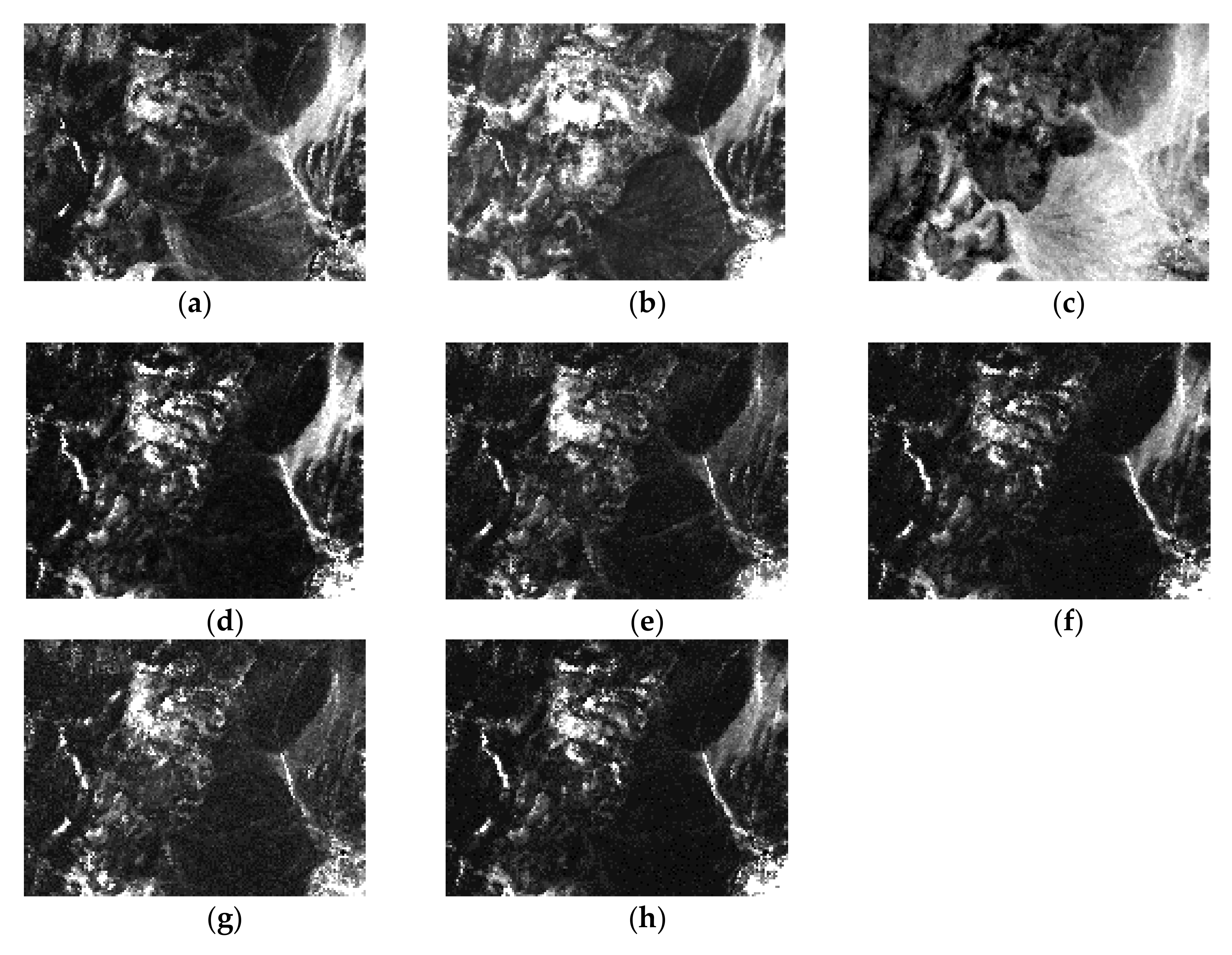
Even if the pixels are highly mixed, the SPEEVD algorithm can obtain reliable results, which is demonstrated not only by the similarity of the spectra, but also in the similarity of the abundance images with the real ground objects’ distribution. The abundance images are shown in Figure 11, Figure 12, Figure 13, Figure 14, Figure 15, Figure 16, Figure 17, Figure 18, Figure 19 and Figure 20. The abundances show good similarities, except for the slight decline in sphene and buddingtonite. All the methods show satisfactory results on kaolinite and alunite, because they are both the prevalent classes in the sub-image. Therefore, the data distribution of the sub-image is prone to these endmembers, which allows each method to distinguish these endmembers much more easily than for the other endmembers which are not prevalent in the sub-image. For the unmixing results, the abundance images in Figure 18 are different: some algorithms extracted chalcedony, while the others did not. The chalcedony, which prevails in the sub-image, is easily visible in ICE, SPICE, and SPEEVD. However, it is missed with the VCA and MVC-NMF methods. This is because VCA is an endmember identification algorithm which searches for pure pixels in the image, whereas the endmember generation methods based on ICE employ an error model with matrix factorization, which can extract endmembers without pure pixels. MVC-NMF performs well in identifying less-prevalent endmembers, but it misses the prevailing endmember, which leads to its relatively large unmixing error.
The RMSE images are shown in Figure 21. If there are some large residuals, especially if they are spatially clustered, this may be an indication that the model does not fit the data adequately. There are two probable causes for this poor fitting. Firstly, the value of μ may not be optimal. Secondly, only MNF transform data is used as the observation data.
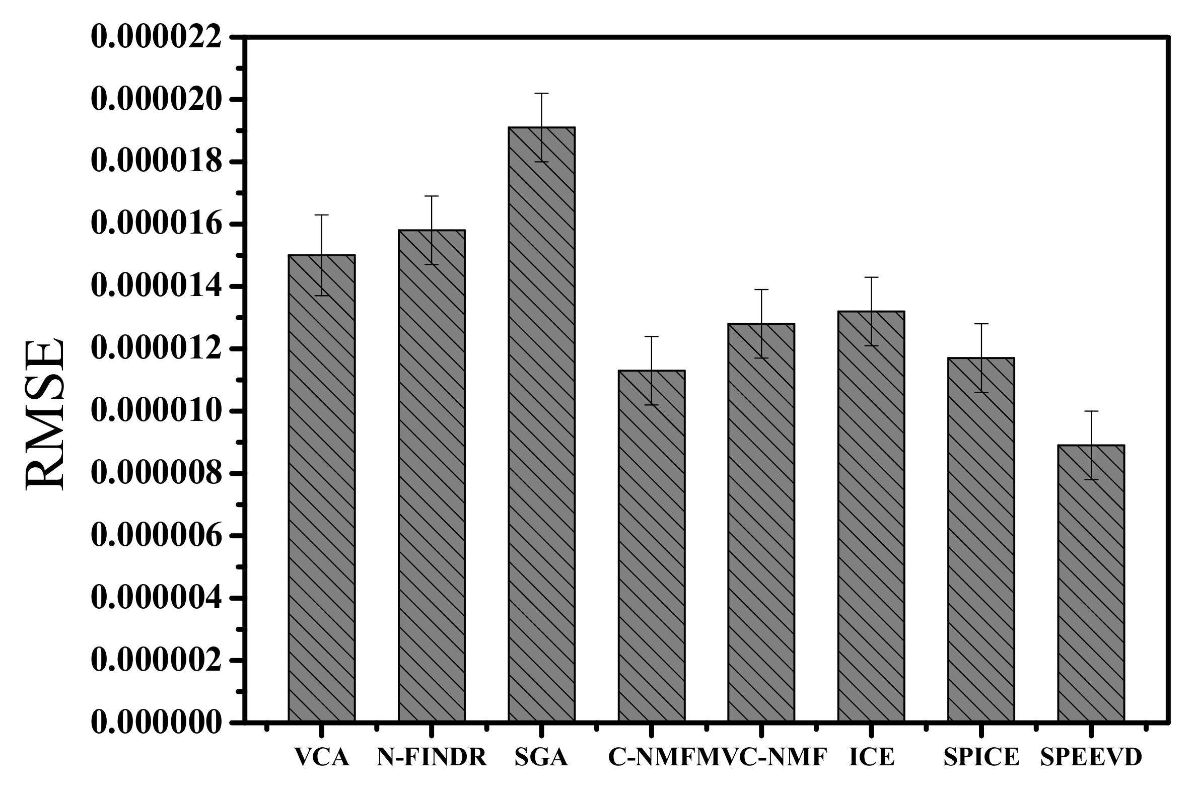
The RMSEs of the unmixing images are shown in Figure 22. Among the different methods, SPEEVD shows the minimum unmixing error, while VCA shows the maximum. The basic assumption of VCA is not satisfied, which leads to its maximum error. The disadvantages of ICE are that it may not find materials that are poorly represented in the scene’s statistics (i.e., outliers that should be identified beforehand), and its error of unmixing is also relatively large. In SPEEVD, although the shortcomings of ICE cannot be eliminated completely, they are suppressed by the volume and deviation constraint. Compared to ICE, which contains only the minimum volume constraint, SPEEVD considers both the volume and deviation constraint. This ensures that the vertices in the MNF transformed space are much closer and more compact and eliminates and excludes the outliers which are not so compact. Moreover, the sparsity constraint on abundances suppresses the distinct outliers which are far from the vertices, which should be considered as noise or abnormals in the MNF transformed space.
The RMSEs of unmixing rely on the fact that the larger the number of endmembers, the smaller the RMSE. However, a large endmember number may lead to a high correlation between the extracted endmembers. The proposed SPEEVD seems to balance the unmixing error and the endmembers’ redundancy, which can be seen in the previous experimental results. If the parameters are suitable, it shows its robustness and minimum error; otherwise, the SPEEVD results may terminate at a number which is larger or smaller than the true endmember number.
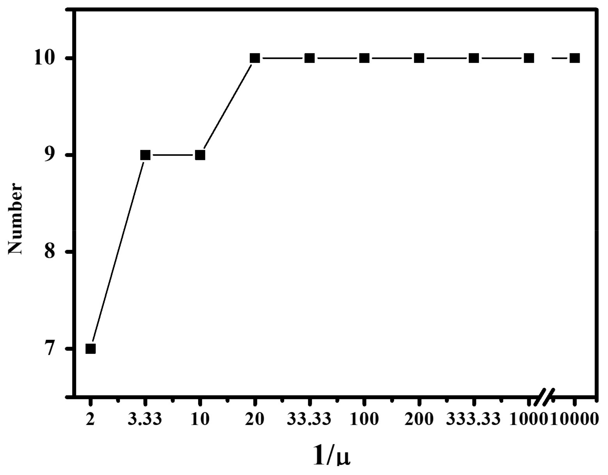
Since the parameters μ and T, which balance the volume constraint and the error model, play an important role in the experiments, we conduct several experiments to obtain the optimal parameter range. The parameter T is set as 0.0001, while the parameter μ is varied from 0.0001 to 0.5. Then, the number of the eventual pruned number is analyzed with the SPEEVD method. The relation between the parameter μ and the eventual number of endmembers is shown in Figure 23.
From the curve in Figure 23, as the parameter μ decreases, the number of the eventual pruned number increases. However, 1/μ = 20, that is μ = 0.05, is an important point, below which the number is stable at ten. Although the parameters μ and T are both related to the number of endmembers, the optimal T has to be decided by the experimental results and is set as 0.0001 in this experiment.
4.3. Experiments with AVIRIS Lunar Crater Volcanic Field Data
The second AVIRIS data set used in this experiment, shown in Figure 24, is from the Lunar Crater volcanic field in Northern Nye County, Nevada, with 120 × 160 pixels and 190 bands after low-SNR and water-absorption bands were removed. The spatial resolution is about 20 m, which means that many pixels are mixed ones. According to prior information in a published paper [49], there are six classes: cinders, playa, rhyolite, shade, dry vegetation, and an anomaly. The Lunar Crater volcanic field local sub-image is also tested with the previously mentioned algorithms.
Since there are no reference spectra in the sub-image, the RMSEs of unmixing in Figure 25 and Figure 26 are used for the assessment metric.
The RMSEs of unmixing in Figure 26 show that SPEEVD performs better than the other methods. Meanwhile, we have tested the time cost of all methods on simulation and real images under Matlab 2009, with windows 7 system, Intel(R) 7 Series Chipset Family SATA AHCI Controller, CPU i5-3210M at 2.5GHz, and DDR is 8G. The simulation image is 100 × 100 pixels with 224 bands, and the real images are the cuprite and lunar images in Section 4.2 and Section 4.3. The time cost of each method is the average of 10 times experiments on each image. The running time results are listed in the following Table 8, Table 9 and Table 10.
Since there is a pruning process, SPEEVD costs slightly more time than ICE. However, the advantage of SPEEVD is that it needs no initial endmember number, while ICE needs an exact endmember number, which is usually difficult to obtain. The time cost of SPEEVD is close to SPICE, due to the quadratic programming, which is a little time consuming. Our future work will focus on reducing the computational cost of SPEEVD.
5. Conclusions
In this paper, an endmember extraction algorithm (SPEEVD) is proposed as an effective automatic endmember extraction method that does not require a predetermined endmember number. Compared to the other state-of-the-art methods, some novel constraints are introduced, with promising experimental results. SPEEVD not only constructs a volume and a deviation constraint by the cross product between endmember vectors, but it also executes a sparse pruning method to adaptively determine the endmembers. A simplified interactive projection gradient method is proposed to solve E, which makes sure that the convergence is steady and saves on computation cost.
Experiments on simulated and real images, which were tested with the VCA, MVC-NMF, ICE, SPICE, and SPEEVD methods, suggest that SPEEVD is effective for automatic endmember extraction. The correlation coefficients and the spectral angle distance were used as similarity metrics for the assessment of the extracted endmember spectra. SPEEVD manifested encouraging results when compared with the other methods.
Several conclusions can be drawn with regard to SPEEVD: (1) the key feature of SPEEVD is that it can adaptively determine the endmember number by a sparse pruning method that drives the endmember number to an appropriate value, without an initial pre-estimated value; (2) the added combined volume and deviation constraint by the cross product between endmembers can weaken the noise interference; (3) the other important feature of SPEEVD is that it generates an RSS map, which is useful for finding outliers and also for estimating the number of endmembers in an image.
Although effective in endmember generation, the optimal parameters of SPEEVD, in this paper, were set by many experiments. How to determine these parameters automatically will be the subject of our further work.
Acknowledgments
This work is jointly supported by the National Natural Science Foundation of China (No. 61301255, 41271432, 41471340, 41301403), the National Key Research and Development Program of China (No. 2017YFB0504200), and the Basic Research Program of Shenzhen (No. JCYJ20150831194441446).
Author Contributions
All the authors made significant contributions to the work. Huali Li and Haicong Yu designed the research model, analyzed the results, and wrote the paper. Jun Liu contributed to the experimental tests, editing and review of the manuscript.
Conflicts of Interest
The authors declare no conflict of interest.
References
- Pan, L.; Li, H.C.; Deng, Y.J.; Zhang, F.; Chen, X.D.; Du, Q. Hyperspectral Dimensionality Reduction by Tensor Sparse and Low-Rank Graph-Based Discriminant Analysis. Remote Sens. 2017, 9, 452. [Google Scholar] [CrossRef]
- Feng, F.B.; Li, W.; Du, Q.; Zhang, B. Dimensionality Reduction of Hyperspectral Image with Graph-Based Discriminant Analysis Considering Spectral Similarity. Remote Sens. 2017, 9, 323. [Google Scholar] [CrossRef]
- Zare, A.; Gader, P. Hyperspectral Band Selection and Endmember Detection Using Sparsity Promoting Priors. IEEE Geosci. Remote Sens. Lett. 2008, 5, 256–260. [Google Scholar] [CrossRef]
- Renard, N.; Bourennane, S. Dimensionality Reduction Based on Tensor Modeling for Classification Methods. IEEE Trans. Geosci. Remote Sens. 2009, 47, 1123–1131. [Google Scholar] [CrossRef]
- Garcia, R.A.; Lee, Z.P.; Hochberg, E.J. Hyperspectral Shallow-Water Remote Sensing with an Enhanced Benthic Classifier. Remote Sens. 2018, 10, 147. [Google Scholar] [CrossRef]
- Du, B.; Zhang, L. Target detection based on a dynamic subspace. Pattern Recogn. 2014, 47, 344–358. [Google Scholar] [CrossRef]
- Du, B.; Zhang, L. Random Selection Based Anomaly Detector for Hyperspectral Imagery. IEEE Trans. Geosci. Remote Sens. 2011, 49, 1578–1589. [Google Scholar] [CrossRef]
- Du, B.; Zhang, L.P. A discriminative metric learning based anomaly detection method. IEEE Trans. Geosci. Remote Sens. 2014, 52, 6844–6857. [Google Scholar]
- Qian, S. Hyperspectral data compression using a fast vector quantization algorithm. IEEE Trans. Geosci. Remote Sens. 2004, 42, 1791–1798. [Google Scholar] [CrossRef]
- Du, Q.; Zhu, W.; Fowler, J.E. Anomaly-Based JPEG2000 Compression of Hyperspectral Imagery. IEEE Trans. Geosci. Remote Sens. 2008, 5, 696–700. [Google Scholar] [CrossRef]
- Lanaras, C.; Baltsavias, E.; Schindler, K. Hyperspectral Super-Resolution with Spectral Unmixing Constraints. Remote Sens. 2017, 9, 1196. [Google Scholar] [CrossRef]
- Rizkinia, M.; Okuda, M. Joint Local Abundance Sparse Unmixing for Hyperspectral Images. Remote Sens. 2017, 9, 1224. [Google Scholar] [CrossRef]
- Feng, R.Y.; Zhong, Y.F.; Wang, L.Z.; Lin, W.J. Rolling Guidance Based Scale-Aware Spatial Sparse Unmixing for Hyperspectral Remote Sensing Imagery. Remote Sens. 2017, 9, 1218. [Google Scholar] [CrossRef]
- Iordache, M.D.; Bioucas-Dias, J.M.; Plaza, A. Sparse Unmixing of Hyperspectral Data. IEEE Trans. Geosci. Remote Sens. 2011, 49, 2014–2039. [Google Scholar] [CrossRef]
- Greer, J.B. Sparse Demixing of Hyperspectral Images. IEEE Trans. Image Process. 2012, 21, 219–228. [Google Scholar] [CrossRef] [PubMed]
- Du, B.; Xiong, W.; Wu, J.; Zhang, L.; Zhang, L.; Tao, D. Stacked Convolutional Denoising Auto-Encoders for Feature Representation. IEEE Trans. Cybern. 2017, 47, 1017–1027. [Google Scholar] [CrossRef] [PubMed]
- Iordache, M.-D.; Bioucas-Dias, J.M.; Plaza, A. Total Variation Spatial Regularization for Sparse Hyperspectral Unmixing. IEEE Trans. Geosci. Remote Sens. 2012, 50, 4484–4502. [Google Scholar] [CrossRef]
- Themelis, K.E.; Rontogiannis, A.A.; Koutroumbas, K.D. A Novel Hierarchical Bayesian Approach for Sparse Semisupervised Hyperspectral Unmixing. IEEE Trans. Signal Process. 2012, 60, 585–599. [Google Scholar] [CrossRef]
- Chen, X.; Chen, J.; Jia, X.; Somers, B.; Wu, J.; Coppin, P. A Quantitative Analysis of Virtual Endmembers' Increased Impact on the Collinearity Effect in Spectral Unmixing. IEEE Trans. Geosci. Remote Sens. 2011, 49, 2945–2956. [Google Scholar] [CrossRef]
- Plaza, J.; Plaza, A.; Martinez, P.; Perez, R. H-COMP: A tool for quantitative and comparative analysis of endmember identification algorithms. Proc. Geosci. Remote Sens. Symp. 2003, 1, 291–293. [Google Scholar]
- Boardman, J.; Kruse, F.; Green, R. Mapping target signatures via partial unmixing of AVIRIS data. In Proceedings of the Summaries JPL Airborne Earth Science Workshop, Pasadena, CA, USA, 23–26 January 1995; pp. 23–26. [Google Scholar]
- Du, B.; Zhang, M.; Zhang, L.; Hu, R.; Tao, D. PLTD: Patch-Based Low-Rank Tensor Decomposition for Hyperspectral Images. IEEE Trans. Multimedia 2017, 19, 67–79. [Google Scholar] [CrossRef]
- Du, B.; Zhang, Y.; Zhang, L.; Tao, D. Beyond the Sparsity-Based Target Detector: A Hybrid Sparsity and Statistics Based Detector for Hyperspectral Images. IEEE Trans. Image Process. 2016, 25, 5345–5357. [Google Scholar] [CrossRef] [PubMed]
- Winter, M.E. N-finder: An algorithm for fast autonomous spectral endmember determination in hyperspectral data. Proc. SPIE 1999, 3753, 266–275. [Google Scholar]
- Nascimento, J.M.P.; Bioucas-Dias, J.M. Vertex component analysis: A fast algorithm to unmix hyperspectral data. IEEE Trans. Geosci. Remote Sens. 2005, 43, 898–910. [Google Scholar] [CrossRef]
- Chang, C.I.; Wu, C.C.; Liu, W.; Ouyang, Y.C. A New Growing Method for Simplex-Based Endmember Extraction Algorithm. IEEE Trans. Geosci. Remote Sens. 2006, 44, 2804–2819. [Google Scholar] [CrossRef]
- Wu, C.C.; Lo, C.S.; Chang, C.I. Improved Process for Use of a Simplex Growing Algorithm for Endmember Extraction. IEEE Geosci. Remote Sens. Lett. 2009, 6, 523–527. [Google Scholar]
- Plaza, A.; Martinez, P.; Perez, R.; Plaza, J. Spatial/Spectral Endmember Extraction by Multidimensional Morphological Operations. IEEE Trans. Geosci. Remote Sens. 2002, 40, 756–770. [Google Scholar] [CrossRef]
- Ifarraguerri, A.; Chang, C.I. Multispectral and hyperspectral image analysis with convex cones. IEEE Trans. Geosci. Remote Sens. 1999, 37, 756–770. [Google Scholar] [CrossRef]
- Craig, M. Minimum volume transforms for remotely sensed data. IEEE Trans. Geosci. Remote Sens. 1994, 32, 542–552. [Google Scholar] [CrossRef]
- Li, J.; Bioucas-Dias, J. Minimum volume simplex analysis: A fast algorithm to unmix hyperspectral data. In Proceedings of the IEEE International Geoscience and Remote Sensing Symposium, Boston, MA, USA, 7–11 July 2008; pp. 2369–2371. [Google Scholar]
- Chan, T.H.; Chi, C.Y.; Huang, Y.M.; Ma, W.K. A Convex Analysis-Based Minimum-Volume Enclosing Simplex Algorithm for Hyperspectral Unmixing. IEEE Trans. Signal Process. 2009, 57, 4418–4432. [Google Scholar] [CrossRef]
- Liu, X.; Xia, W.; Wang, B.; Zhang, L. An approach based on constrained nonnegative matrix factorization to unmix hyperspectral data. IEEE Trans. Geosci. Remote Sens. 2011, 49, 757–772. [Google Scholar] [CrossRef]
- Jia, S.; Qian, Y. Constrained nonnegative matrix factorization for hyperspectral unmixing. IEEE Trans. Geosci. Remote Sens. 2009, 47, 161–173. [Google Scholar] [CrossRef]
- Parra, L.C.; Sajda, P.; Du, S. Recovery of constituent spectra using non-negative matrix factorization. Proc. SPIE 2003, 1, 321–331. [Google Scholar]
- Miao, L.; Qi, H. Endmember extraction from highly mixed data using minimum volume constrained nonnegative matrix factorization. IEEE Trans. Geosci. Remote Sens. 2007, 45, 765–777. [Google Scholar] [CrossRef]
- Bioucas-Dias, M. A variable splitting augmented Lagrangian approach to linear spectral unmixing. In Proceedings of the First Workshop on Hyperspectral Image and Signal Processing: Evolution in Remote Sensing, Grenoble, France, 26–28 August 2009; pp. 1–4. [Google Scholar]
- Neville, R.A.; Staenz, K.; Szeredi, T.; Lefebvre, J.; Hauff, P. Automatic endmember extraction from hyperspectral data for mineral exploration. In Proceedings of the 21st Canadian Symposium Remote Sensing, Ottawa, ON, Canada, 21–24 June 1999; pp. 21–24. [Google Scholar]
- Li, H.; Zhang, L. A Hybrid Automatic Endmember Extraction Algorithm Based on a Local Window. IEEE Trans. Geosci. Remote Sens. 2011, 49, 4223–4238. [Google Scholar] [CrossRef]
- Berman, M.; Kiiveri, H.; Lagerstrom, R.; Ernst, A.; Dunne, R.; Huntington, J.F. ICE: A statistical approach to identifying endmembers in hyperspectral images. IEEE Trans. Geosci. Remote Sens. 2004, 42, 2085–2095. [Google Scholar] [CrossRef]
- Zare, A.; Gader, P. Sparsity Promoting Iterated Constrained Endmember Detection in Hyperspectral Imagery. IEEE Geosci. Remote Sens. Lett. 2007, 4, 446–450. [Google Scholar] [CrossRef]
- Yang, Z.; Zhou, G.; Xie, S.; Ding, S.; Yang, J.; Zhang, J. Blind Spectral Unmixing Based on Sparse Nonnegative Matrix Factorization. IEEE Trans. Image Process. 2011, 20, 1112–1125. [Google Scholar] [CrossRef] [PubMed]
- Lu, X.; Wu, H.; Yuan, Y.; Yan, P.; Li, X. Manifold Regularized Sparse NMF for Hyperspectral Unmixing. IEEE Trans. Geosci. Remote Sens. 2012, 99, 1–12. [Google Scholar] [CrossRef]
- Chang, C.I.; Du, Q. Estimation of Number of Spectrally Distinct Signal Sources in Hyperspectral Imagery. IEEE Trans. Geosci. Remote Sens. 2004, 42, 608–619. [Google Scholar] [CrossRef]
- Bajorski, P. Second Moment Linear Dimensionality as an Alternative to Virtual Dimensionality. IEEE Trans. Geosci. Remote Sens. 2011, 49, 672–678. [Google Scholar] [CrossRef]
- Luo, B.; Chanussot, J.; Douté, S. Unsupervised endmember extraction: Application to hyperspectral images from Mars. In Proceedings of the 2009 16th IEEE International Conference on Image Processing (ICIP), Cairo, Egypt, 7–10 November 2009. [Google Scholar]
- Bioucas-Dias, J.M.; Nascimento, J.M.P. Hyperspectral Subspace Identification. IEEE Trans. Geosci. Remote Sens. 2008, 46, 2435–2445. [Google Scholar] [CrossRef]
- Kuybeda, O.; Malah, D.; Barzohar, M. Rank estimation and redundancy reduction of high-dimensional noisy signals with preservation of rare vectors. IEEE Trans. Signal Process. 2007, 55, 5579–5592. [Google Scholar] [CrossRef]
- Acito, N.; Diani, M.; Corsini, G. Hyperspectral Signal Subspace Identification in the presence of rare signal components. IEEE Trans. Geosci. Remote Sens. 2010, 48, 1940–1954. [Google Scholar] [CrossRef]
- Fukunaga, K. Intrinsic dimensionality extraction. Classif. Pattern Recognit. Reduct. Dimens. 1982, 2, 347–360. [Google Scholar]
- Lee, D.; Seung, H.S. Algorithms for Non-Negative Matrix Factorization. Available online: https://papers.nips.cc/paper/1861-algorithms-for-non-negative-matrix-factorization.pdf (accessed on 1 March 2018).
- Hoyer, P.O. Non-negative Matrix Factorization with Sparseness Constraints. J. Mach. Learn. Res. 2004, 5, 1457–1469. [Google Scholar]
- Li, C.; Ma, Y.; Mei, X.G.; Fan, F.; Huang, J.; Ma, J.Y. Sparse Unmixing of Hyperspectral Data with Noise Level Estimation. Remote Sens. 2017, 9, 1166. [Google Scholar] [CrossRef]
- Leon, S.J. Linear Algebra with Applications, 7th ed.; China Machine Press: Beijing, China, 2009. [Google Scholar]
- Figueiredo, M.A.T. Adaptive sparseness for supervised learning. IEEE Trans. Pattern Anal. Mach. Intell. 2003, 25, 1150–1159. [Google Scholar] [CrossRef]
- Casazza, P.G.; Heinecke, A.; Krahmer, F.; Kutyniok, G. Optimally Sparse Frames. IEEE Trans. Inf. Theory 2011, 99, 1–16. [Google Scholar] [CrossRef]
- Williams, P. Bayesian regularization and pruning using a Laplace prior. Neural Comput. 1995, 7, 117–143. [Google Scholar] [CrossRef]
- USGS Spectroscopy Lab. Cuprite, Nevada, AVIRIS 1995 Data. Available online: http://speclab.cr.usgs.gov/cuprite95.1um_map.tgif.gif (accessed on 1 March 2018).
- Hendrix, E.M.T.; Garcia, I.; Plaza, J.; Martin, G.; Plaza, A. A New Minimum-Volume Enclosing Algorithm for Endmember Identification and Abundance Estimation in Hyperspectral Data. IEEE Trans. Geosci. Remote Sens. 2012, 50, 2744–2757. [Google Scholar] [CrossRef]
Figure 1.
An example of solution uncertainty.

Figure 2.
An example of solution uncertainty (with convex description).

Figure 3.
Obtaining the initial value of M with the SPEEVD method.

Figure 4.
Spectra of five minerals with the different methods: (a) Carnallite, (b) Chlorite, (c) Clinochlore, (d) Clintonite, (e) Corundum.
Figure 4.
Spectra of five minerals with the different methods: (a) Carnallite, (b) Chlorite, (c) Clinochlore, (d) Clintonite, (e) Corundum.

Figure 5.
The average RMSEs of unmixing.

Figure 6.
Correlation coefficients with different SNR levels. (a) Carnallite (b) Chlorite (c) Clinochlore (d) Clintonite (e) Corundum.
Figure 6.
Correlation coefficients with different SNR levels. (a) Carnallite (b) Chlorite (c) Clinochlore (d) Clintonite (e) Corundum.


Figure 7.
Correlation coefficients with different purities: (a) Carnallite, (b) Chlorite, (c) Clinochlore, (d) Clintonite, (e) Corundum.
Figure 7.
Correlation coefficients with different purities: (a) Carnallite, (b) Chlorite, (c) Clinochlore, (d) Clintonite, (e) Corundum.

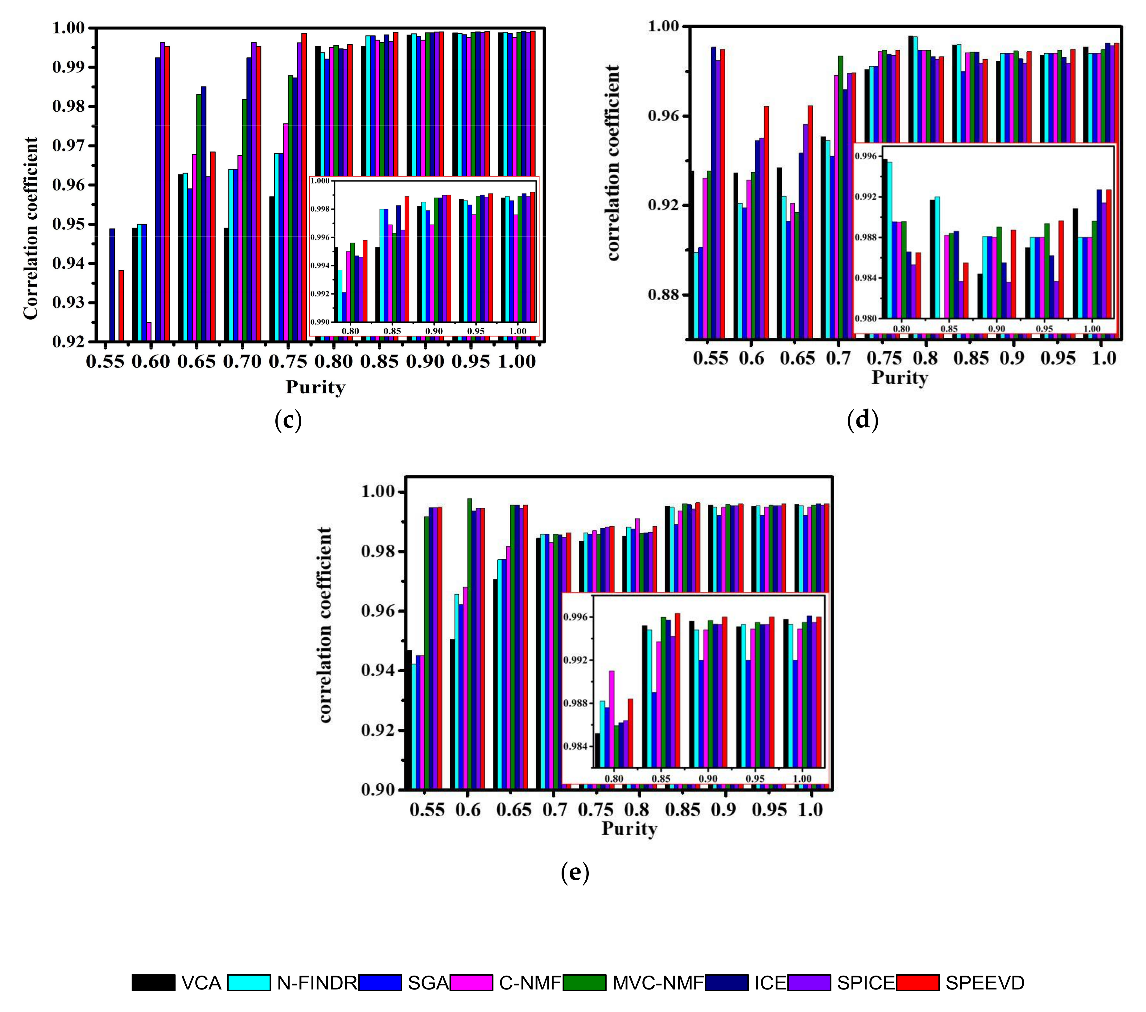
Figure 8.
The RMSE of unmixing.

Figure 9.
Sub-image of AVIRIS data. (a) Sub-image of AVIRIS data (R 2.10 µm, G 2.20µm, B 2.34 µm); (b) USGS 1995 Nevada Cuprite reference map.
Figure 9.
Sub-image of AVIRIS data. (a) Sub-image of AVIRIS data (R 2.10 µm, G 2.20µm, B 2.34 µm); (b) USGS 1995 Nevada Cuprite reference map.
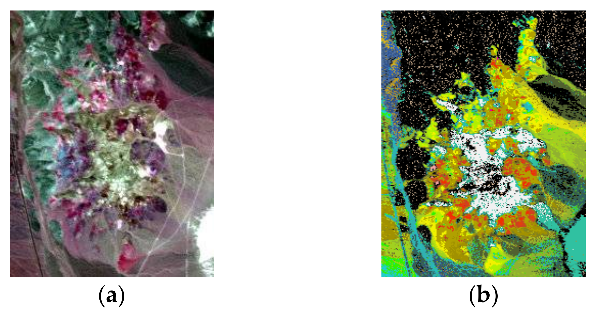
Figure 10.
Endmember spectra with the different methods. (a) alunite (b) sphene (c) calcite (d) muscovite (e) montmorillonite (f) desert vanish (g) buddingtonite (h) chalcedony (i) kaolinite KGA (j) jarosite.
Figure 10.
Endmember spectra with the different methods. (a) alunite (b) sphene (c) calcite (d) muscovite (e) montmorillonite (f) desert vanish (g) buddingtonite (h) chalcedony (i) kaolinite KGA (j) jarosite.
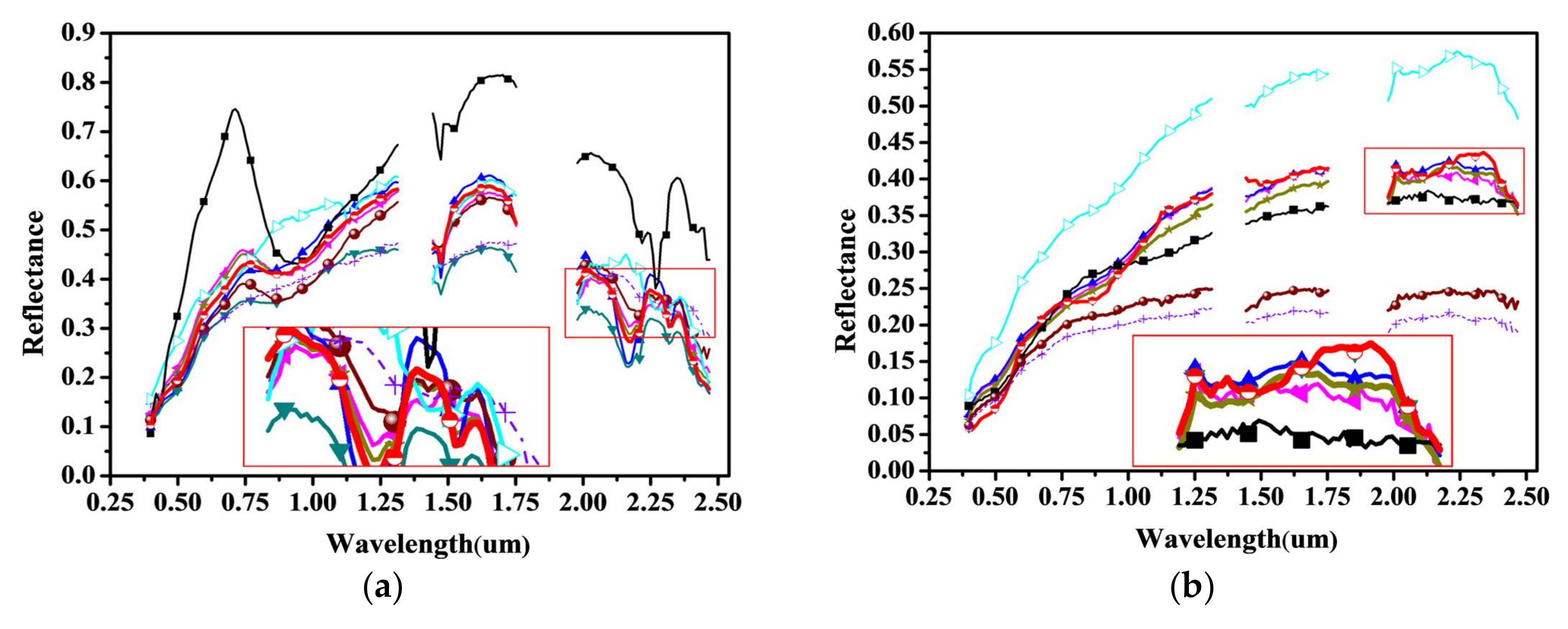

Figure 11.
Alunite: (a) VCA, (b) N-FINDR, (c) SGA, (d) C-NMF, (e) MVC-NMF, (f) ICE, (g) SPICE, (h) SPEEVD.
Figure 11.
Alunite: (a) VCA, (b) N-FINDR, (c) SGA, (d) C-NMF, (e) MVC-NMF, (f) ICE, (g) SPICE, (h) SPEEVD.

Figure 12.
Sphene: (a) VCA, (b) N-FINDR, (c)SGA, (d) C-NMF, (e) MVC-NMF, (f) ICE, (g) SPICE, (h) SPEEVD.
Figure 12.
Sphene: (a) VCA, (b) N-FINDR, (c)SGA, (d) C-NMF, (e) MVC-NMF, (f) ICE, (g) SPICE, (h) SPEEVD.

Figure 13.
Calcite: (a) VCA, (b) N-FINDR, (c) SGA, (d) C-NMF, (e) MVC-NMF, (f) ICE, (g) SPICE, (h) SPEEVD.
Figure 13.
Calcite: (a) VCA, (b) N-FINDR, (c) SGA, (d) C-NMF, (e) MVC-NMF, (f) ICE, (g) SPICE, (h) SPEEVD.
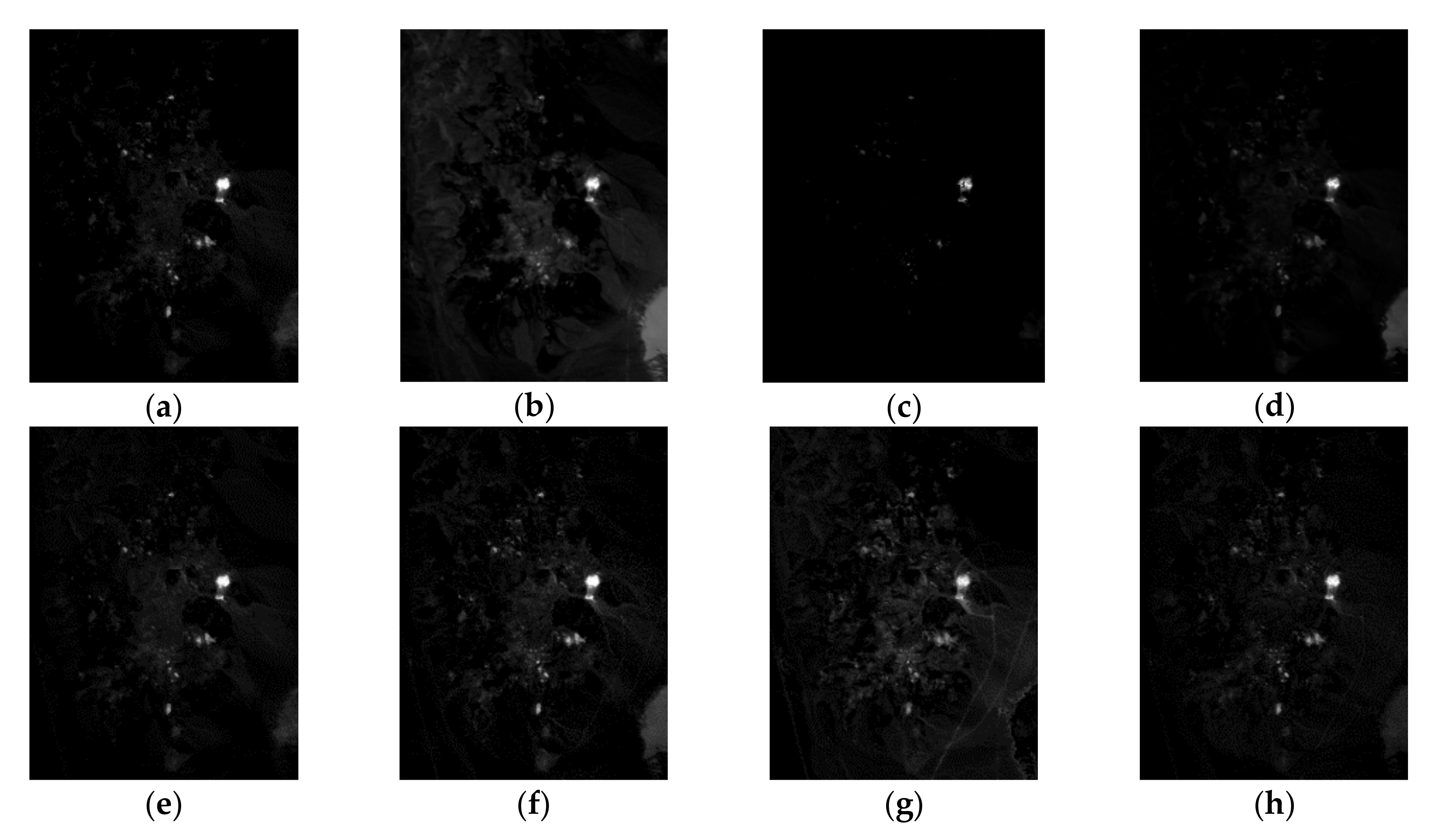
Figure 14.
Muscovite: (a) VCA, (b) N-FINDR, (c) SGA, (d) C-NMF, (e) MVC-NMF, (f) ICE, (g) SPICE, (h) SPEEVD.
Figure 14.
Muscovite: (a) VCA, (b) N-FINDR, (c) SGA, (d) C-NMF, (e) MVC-NMF, (f) ICE, (g) SPICE, (h) SPEEVD.

Figure 15.
Montmorillonite: (a) VCA, (b) N-FINDR, (c) SGA, (d) C-NMF, (e) MVC-NMF, (f) ICE, (g) SPICE, (h) SPEEVD.
Figure 15.
Montmorillonite: (a) VCA, (b) N-FINDR, (c) SGA, (d) C-NMF, (e) MVC-NMF, (f) ICE, (g) SPICE, (h) SPEEVD.
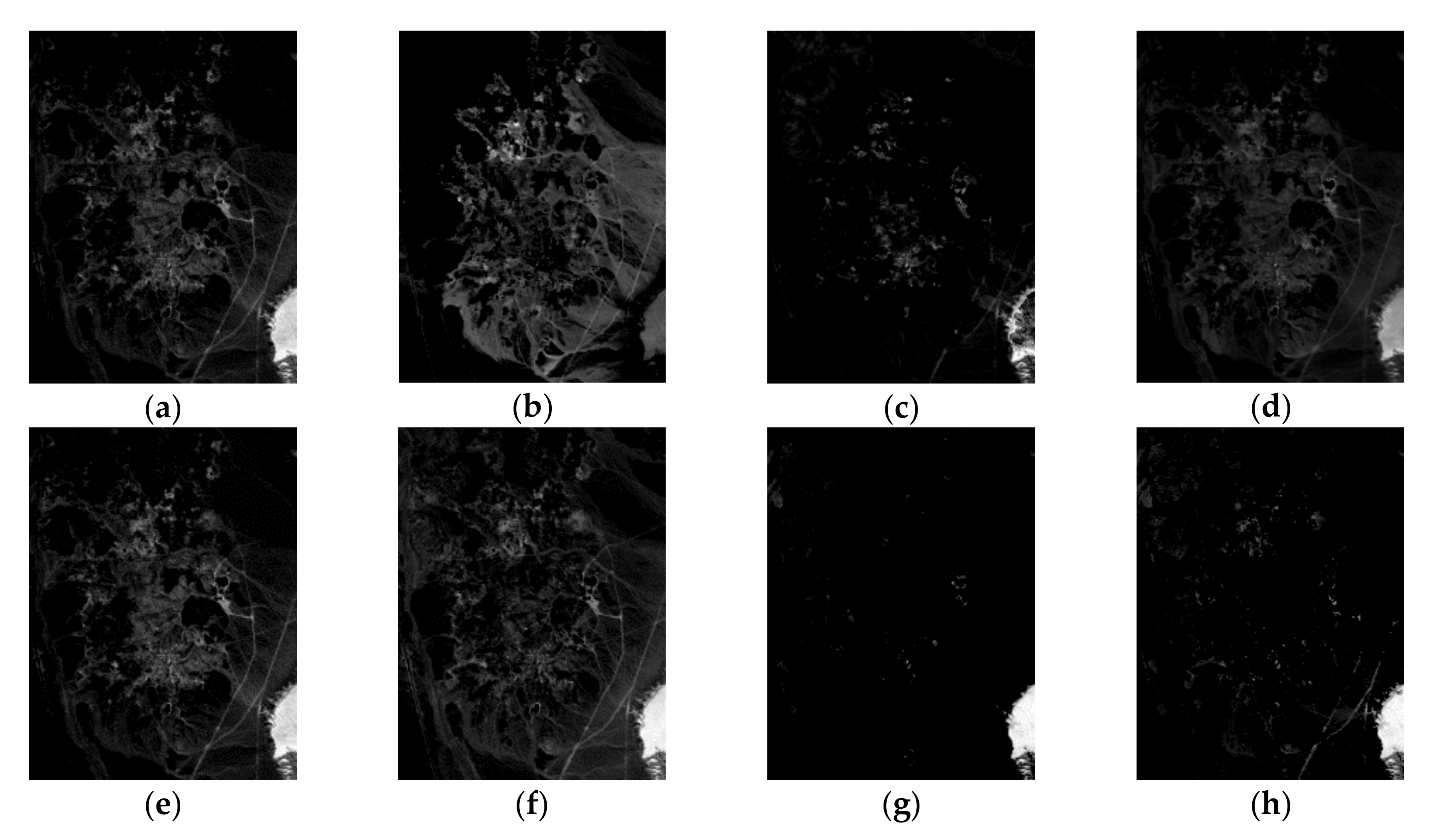
Figure 16.
Desert varnish: (a) VCA, (b) N-FINDR, (c) SGA, (d) C-NMF, (e) MVC-NMF, (f) ICE, (g) SPICE, (h) SPEEVD.
Figure 16.
Desert varnish: (a) VCA, (b) N-FINDR, (c) SGA, (d) C-NMF, (e) MVC-NMF, (f) ICE, (g) SPICE, (h) SPEEVD.

Figure 17.
Buddingtonite: (a) VCA, (b) N-FINDR, (c) SGA, (d) C-NMF, (e) MVC-NMF, (f) ICE, (g) SPICE, (h) SPEEVD.
Figure 17.
Buddingtonite: (a) VCA, (b) N-FINDR, (c) SGA, (d) C-NMF, (e) MVC-NMF, (f) ICE, (g) SPICE, (h) SPEEVD.

Figure 18.
Chalcedony: (a) VCA, (b) N-FINDR, (c) SGA, (d) C-NMF, (e) MVC-NMF, (f) ICE, (g) SPICE, (h) SPEEVD.
Figure 18.
Chalcedony: (a) VCA, (b) N-FINDR, (c) SGA, (d) C-NMF, (e) MVC-NMF, (f) ICE, (g) SPICE, (h) SPEEVD.

Figure 19.
Kaolinite KGA: (a) VCA, (b) N-FINDR, (c) SGA, (d) C-NMF, (e) MVC-NMF, (f) ICE, (g) SPICE, (h) SPEEVD.
Figure 19.
Kaolinite KGA: (a) VCA, (b) N-FINDR, (c) SGA, (d) C-NMF, (e) MVC-NMF, (f) ICE, (g) SPICE, (h) SPEEVD.

Figure 20.
Jarosite + alunite 4: (a) VCA, (b) N-FINDR, (c) SGA, (d) C-NMF, (e) MVC-NMF, (f) ICE, (g) SPICE, (h) SPEEVD.
Figure 20.
Jarosite + alunite 4: (a) VCA, (b) N-FINDR, (c) SGA, (d) C-NMF, (e) MVC-NMF, (f) ICE, (g) SPICE, (h) SPEEVD.

Figure 21.
RMSE images: (a) VCA, (b) N-FINDR, (c) SGA, (d) C-NMF, (e) MVC-NMF, (f) ICE, (g) SPICE, (h) SPEEVD.
Figure 21.
RMSE images: (a) VCA, (b) N-FINDR, (c) SGA, (d) C-NMF, (e) MVC-NMF, (f) ICE, (g) SPICE, (h) SPEEVD.

Figure 22.
The RMSEs of the unmixing results.
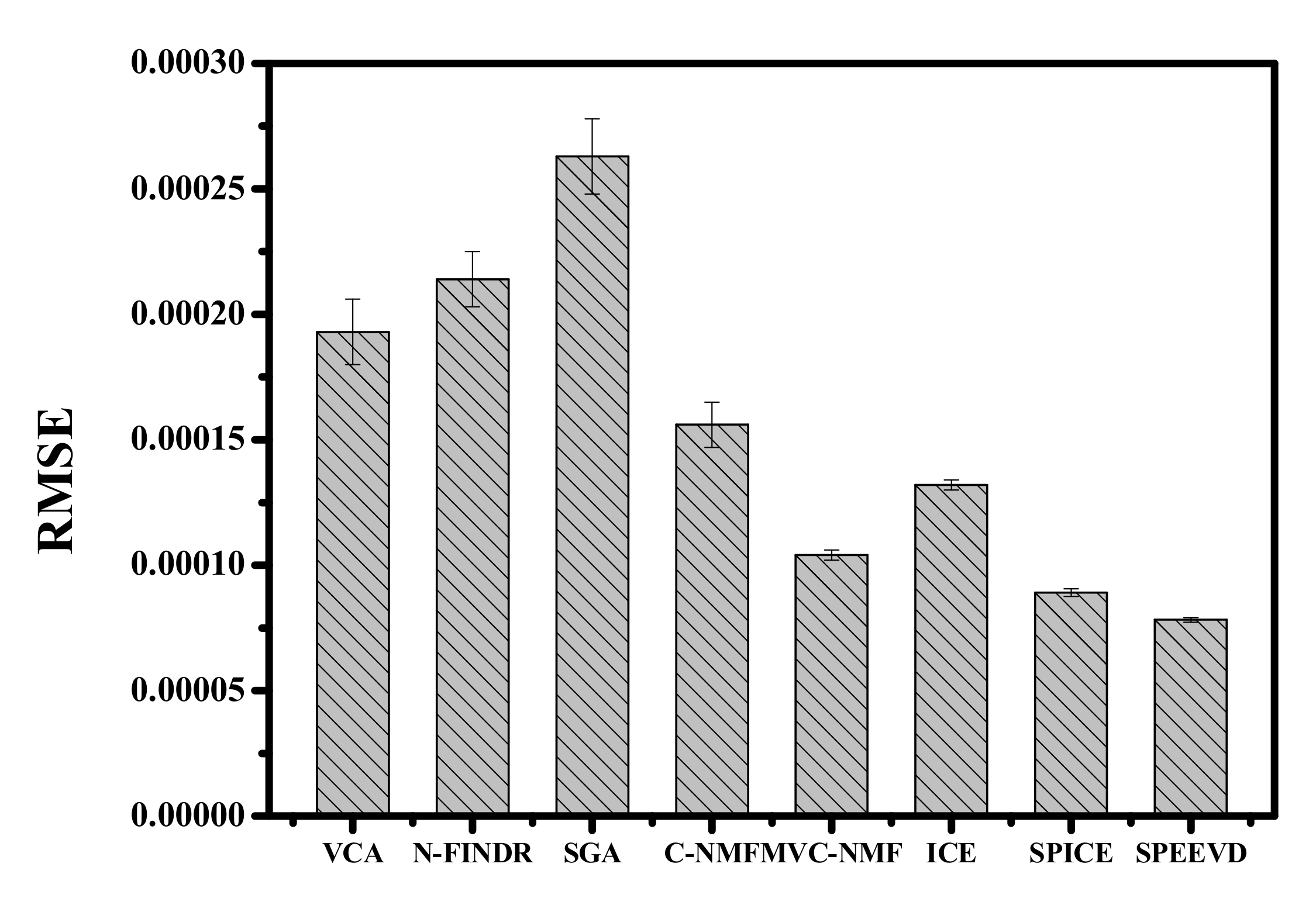
Figure 23.
The parameter μ and the number of endmembers.

Figure 24.
The sub-image of rotated LCVF (R 1453.49 nm, G 990.25 nm, B 547.20 nm).
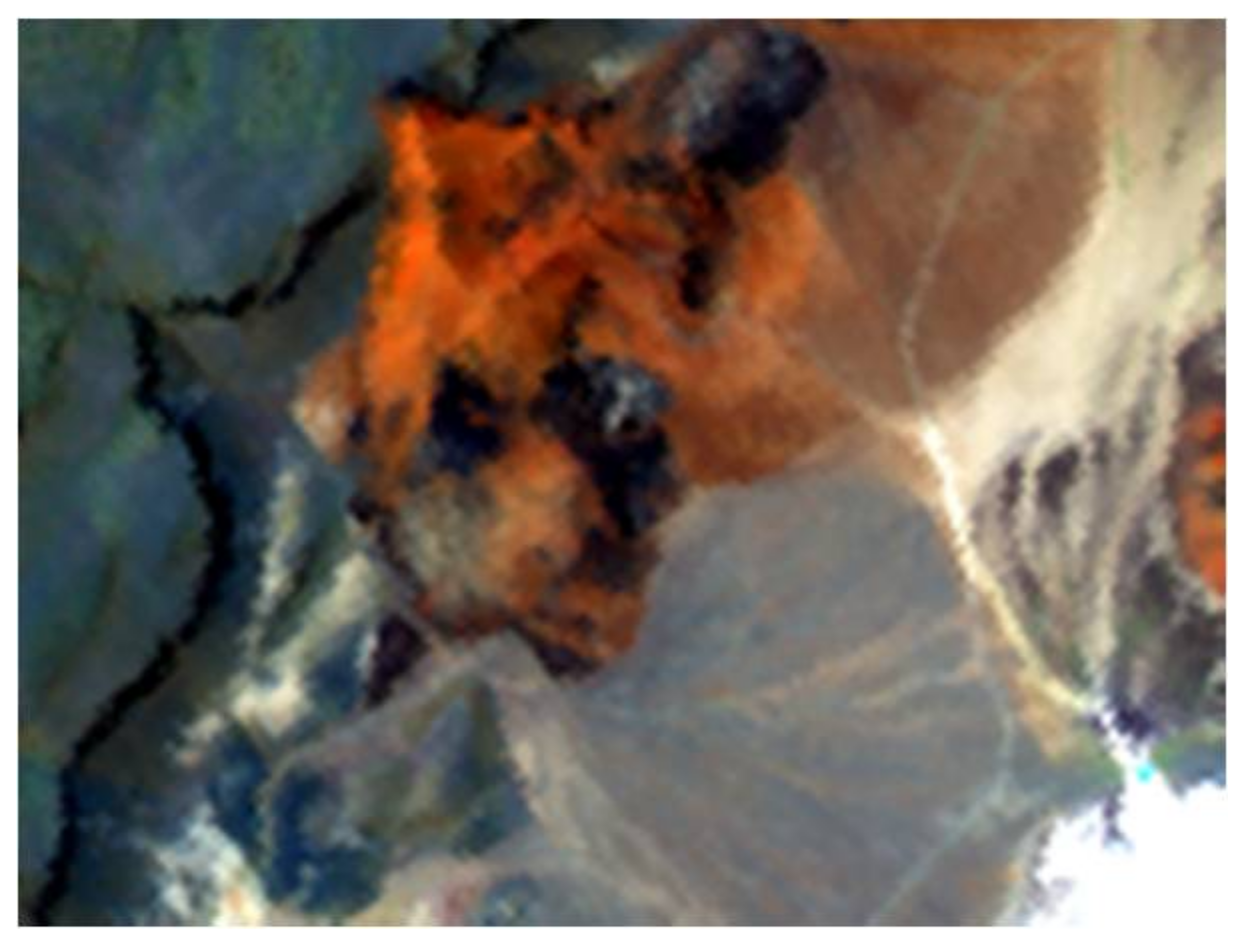
Figure 25.
The unmixing RMSEs: (a) VCA, (b) N-FINDR, (c) SGA, (d) C-NMF, (e) MVC-NMF, (f) ICE, (g) SPICE, (h) SPEEVD.
Figure 25.
The unmixing RMSEs: (a) VCA, (b) N-FINDR, (c) SGA, (d) C-NMF, (e) MVC-NMF, (f) ICE, (g) SPICE, (h) SPEEVD.

Figure 26.
The RMSEs of unmixing with the various methods.


Table 1.
The correlation coefficients between the extracted endmembers and the USGS library spectra.
Table 1.
The correlation coefficients between the extracted endmembers and the USGS library spectra.
| Correlation | VCA | N-FINDR | SGA | C-NMF | MVC-NMF | ICE | SPICE | SPEEVD |
|---|---|---|---|---|---|---|---|---|
| Coefficient | ||||||||
| Carnallite | 0.9987 | 0.9982 | 0.9972 | 0.9989 | 0.9989 | 0.9986 | 0.9988 | 0.9991 |
| Chlorite | 0.9979 | 0.9980 | 0.9980 | 0.9987 | 0.9983 | 0.9978 | 0.9992 | 0.9993 |
| Clinochlore | 0.9964 | 0.9889 | 0.9785 | 0.9970 | 0.9972 | 0.9970 | 0.9972 | 0.9974 |
| Clintonite | 0.9035 | 0.9045 | 0.9088 | 0.9840 | 0.9986 | 0.9269 | 0.9846 | 0.9981 |
| Corundum | 0.9971 | 0.9961 | 0.9689 | 0.9980 | 0.9978 | 0.9961 | 0.9970 | 0.9978 |
Table 2.
The cosine of SAD values between the extracted endmembers and the USGS library.
| Cos(SAD) | VCA | N-FINDR | SGA | C-NMF | MVC-NMF | ICE | SPICE | SPEEVD |
|---|---|---|---|---|---|---|---|---|
| Carnallite | 0.9984 | 0.9983 | 0.9980 | 0.9991 | 0.9991 | 0.9984 | 0.9987 | 0.9993 |
| Chlorite | 0.9988 | 0.9981 | 0.9981 | 0.9993 | 0.9989 | 0.9984 | 0.9982 | 0.9994 |
| Clinochlore | 0.9998 | 0.9989 | 0.9894 | 0.9999 | 0.9999 | 0.9998 | 0.9998 | 0.9999 |
| Clintonite | 0.9962 | 0.9937 | 0.9656 | 0.9992 | 0.9999 | 0.9963 | 0.9965 | 0.9989 |
| Corundum | 0.9997 | 0.9989 | 0.9979 | 0.9998 | 0.9998 | 0.9996 | 0.9998 | 0.9999 |
Table 3.
SID-SAD metric values between the extracted endmembers and the USGS library.
| SID-SAD | VCA | N-FINDR | SGA | C-NMF | MVC-NMF | ICE | SPICE | SPEEVD |
|---|---|---|---|---|---|---|---|---|
| Carnallite | 24.5356 | 24.5356 | 49.1908 | 22.0654 | 20.1549 | 46.6332 | 24.4198 | 22.8277 |
| Chlorite | 8.4406 | 8.6724 | 8.6744 | 5.6652 | 8.3581 | 8.3730 | 8.2069 | 5.4573 |
| Clinochlore | 0.1819 | 0.1994 | 1.3178 | 0.1540 | 0.1605 | 0.1701 | 0.1816 | 0.1514 |
| Clintonite | 26.0397 | 27.9036 | 19.5728 | 15.8640 | 14.7124 | 17.6472 | 16.2487 | 15.7286 |
| Corundum | 0.9892 | 2.3918 | 3.1188 | 0.5895 | 0.5878 | 0.5961 | 0.9701 | 0.5254 |
Table 4.
The results of estimated endmember number with different parameters.
| Three Group of Parameters | |||
|---|---|---|---|
| μ | 0.00005 | 0.0001 | 0.0002 |
| T | 0.0001 | 0.0001 | 0.0001 |
| Estimated number | 5 | 5 | 5 |
Table 5.
The average correlation coefficient between the extracted endmember and USGS library spectra.
Table 5.
The average correlation coefficient between the extracted endmember and USGS library spectra.
| Method | VCA | N-FINDR | SGA | C-NMF | MVC-NMF | ICE | SPICE | SPEEVD |
|---|---|---|---|---|---|---|---|---|
| Correlation | 0.8023 | 0.8157 | 0.7863 | 0.9682 | 0.9789 | 0.9436 | 0.9793 | 0.9813 |
| Coefficient |
Table 6.
The cosine of SAD values between the extracted endmember and the USGS library spectra.
| Method | VCA | N-FINDR | SGA | C-NMF | MVC-NMF | ICE | SPICE | SPEEVD |
|---|---|---|---|---|---|---|---|---|
| Cos(SAD) | 0.9073 | 0.8961 | 0.8174 | 0.9523 | 0.9915 | 0.9668 | 0.9877 | 0.9937 |
Table 7.
The average SID-SAD between the extracted endmember and the USGS library spectra.
| Method | VCA | N-FINDR | SGA | C-NMF | MVC-NMF | ICE | SPICE | SPEEVD |
|---|---|---|---|---|---|---|---|---|
| SID-SAD | 12.9073 | 14.8157 | 20.7863 | 10.9682 | 10.9519 | 10.9668 | 10.9707 | 10.9376 |
Table 8.
The average running time of all methods on simulation image.
| Time Cost | VCA | N-FINDR | SGA | C-NMF | MVC-NMF | ICE | SPICE | SPEEVD |
|---|---|---|---|---|---|---|---|---|
| seconds | 3.08 | 112.3 | 3.45 | 31.4 | 45.36 | 19.3 | 39.5 | 47.74 |
Table 9.
The average running time of all methods on Cuprite image.
| Time Cost | VCA | N-FINDR | SGA | C-NMF | MVC-NMF | ICE | SPICE | SPEEVD |
|---|---|---|---|---|---|---|---|---|
| seconds | 18.46 | 712.1 | 25.2 | 313.6 | 458.6 | 334.2 | 398.3 | 506.8 |
Table 10.
The average running time of all methods on Lunar image.
| Time Cost | VCA | N-FINDR | SGA | C-NMF | MVC-NMF | ICE | SPICE | SPEEVD |
|---|---|---|---|---|---|---|---|---|
| seconds | 4.198 | 217.3 | 7.16 | 161.83 | 152.6 | 79.3 | 113.3 | 174.26 |
© 2018 by the authors. Licensee MDPI, Basel, Switzerland. This article is an open access article distributed under the terms and conditions of the Creative Commons Attribution (CC BY) license (http://creativecommons.org/licenses/by/4.0/).
Share and Cite
MDPI and ACS Style
Li, H.; Liu, J.; Yu, H. An Automatic Sparse Pruning Endmember Extraction Algorithm with a Combined Minimum Volume and Deviation Constraint. Remote Sens. 2018, 10, 509. https://doi.org/10.3390/rs10040509
AMA Style
Li H, Liu J, Yu H. An Automatic Sparse Pruning Endmember Extraction Algorithm with a Combined Minimum Volume and Deviation Constraint. Remote Sensing. 2018; 10(4):509. https://doi.org/10.3390/rs10040509
Chicago/Turabian StyleLi, Huali, Jun Liu, and Haicong Yu. 2018. "An Automatic Sparse Pruning Endmember Extraction Algorithm with a Combined Minimum Volume and Deviation Constraint" Remote Sensing 10, no. 4: 509. https://doi.org/10.3390/rs10040509
Note that from the first issue of 2016, this journal uses article numbers instead of page numbers. See further details here.