A Unified Algorithm for Channel Imbalance and Antenna Phase Center Position Calibration of a Single-Pass Multi-Baseline TomoSAR System


Abstract
:
1. Introduction
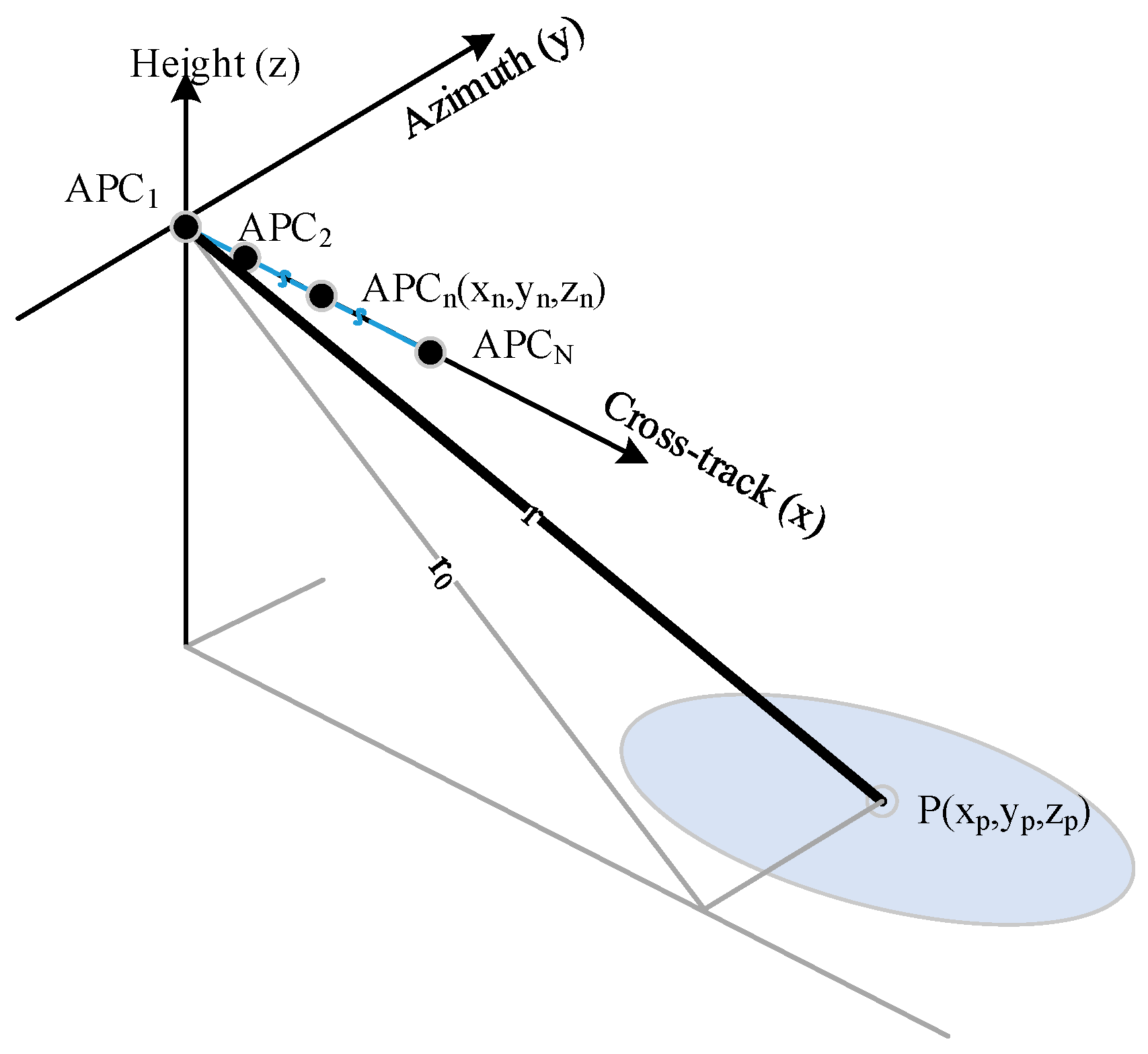
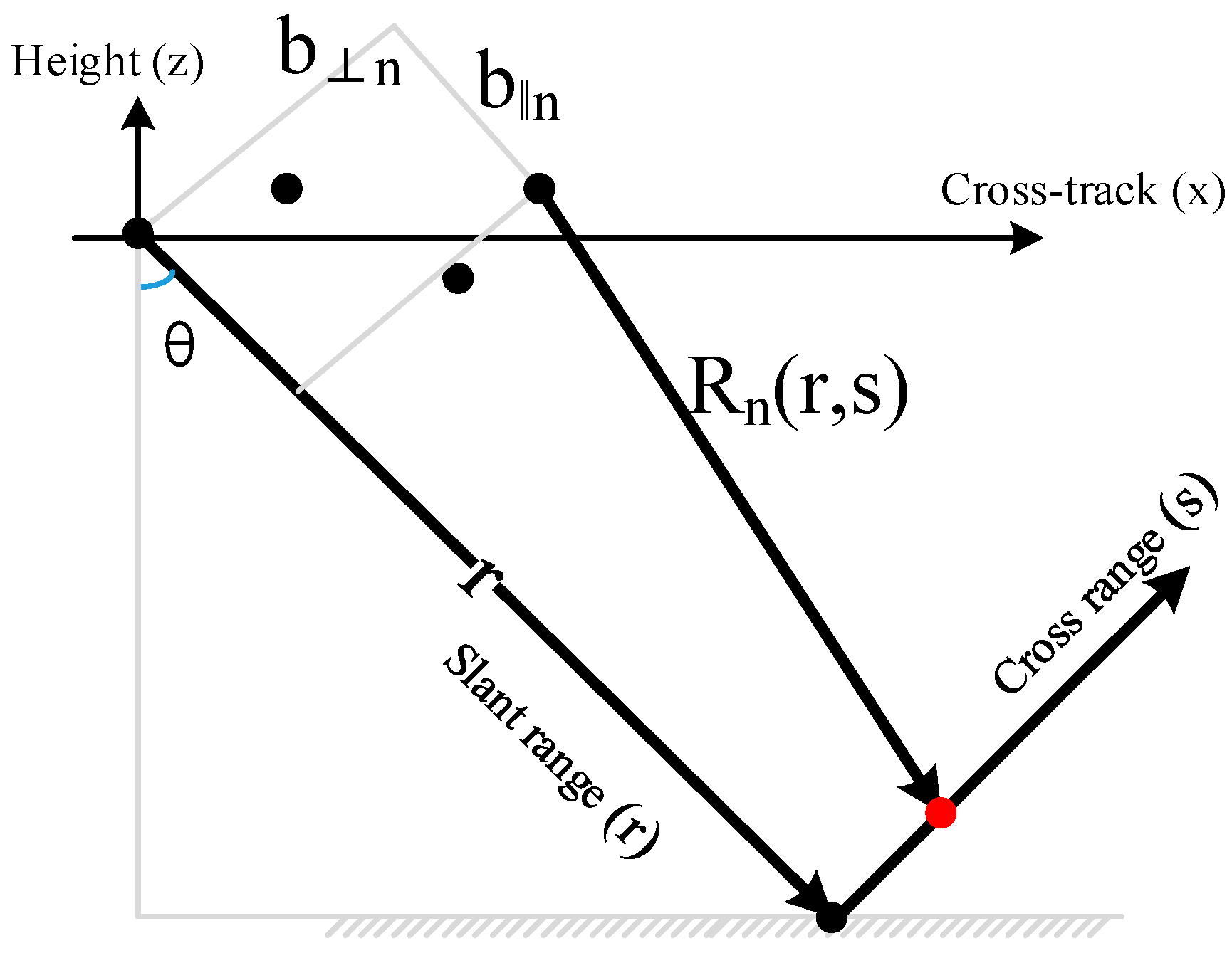
2. A Signal Model
3. The Calibration Algorithm
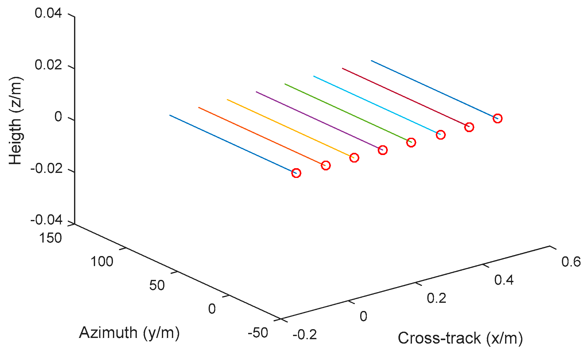
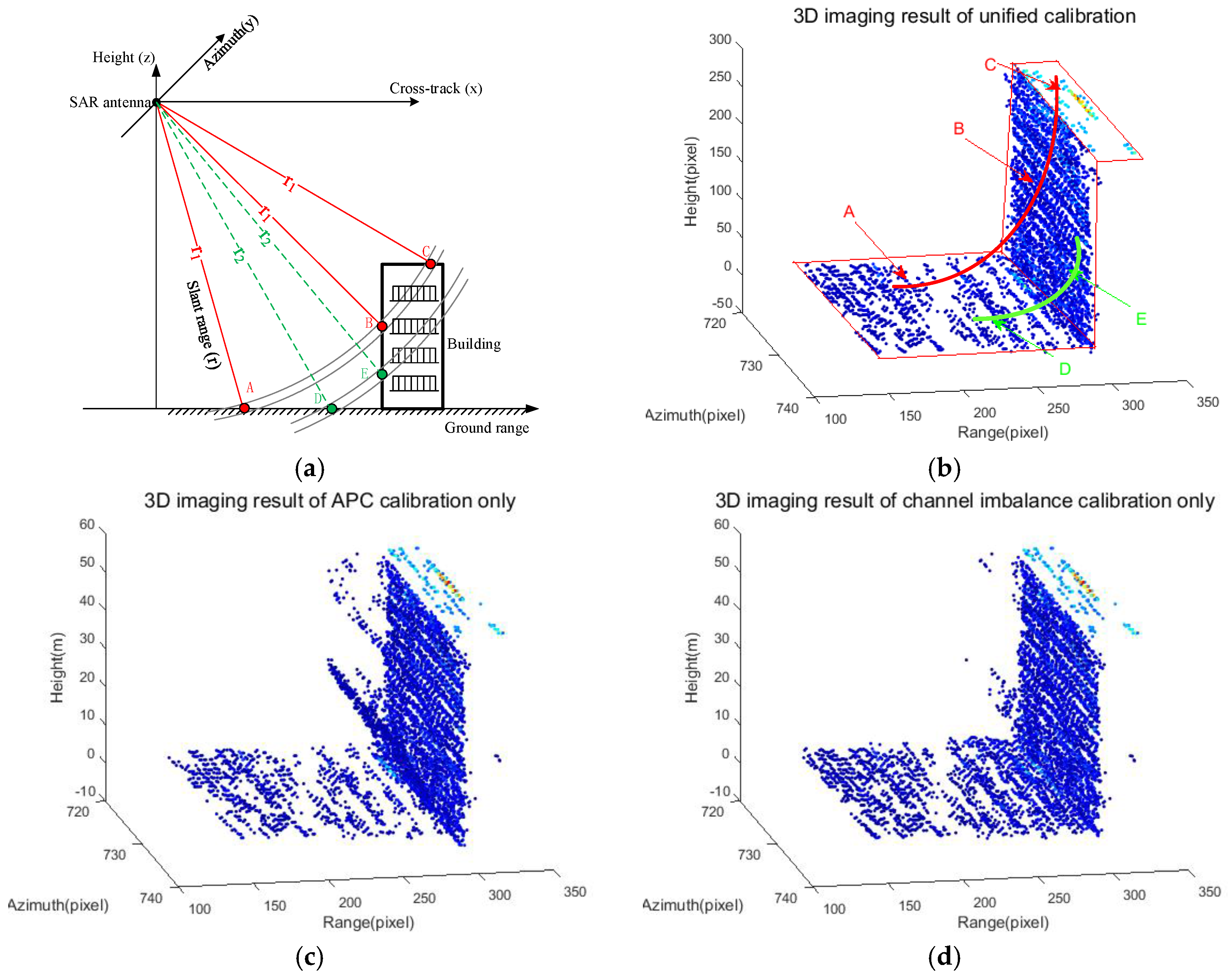
3.1. Step 1: APC Position Calibration
3.2. Step 2: Channel Imbalance Calibration
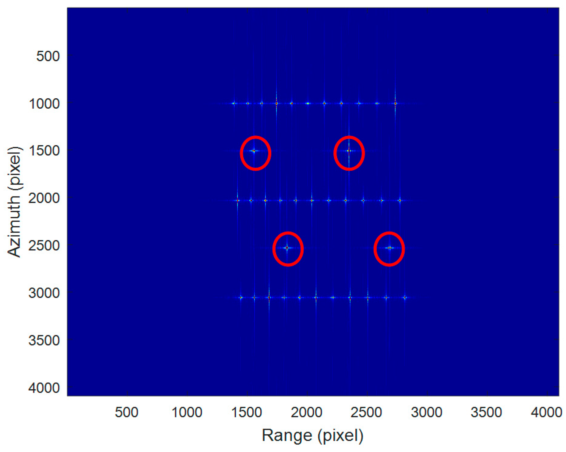
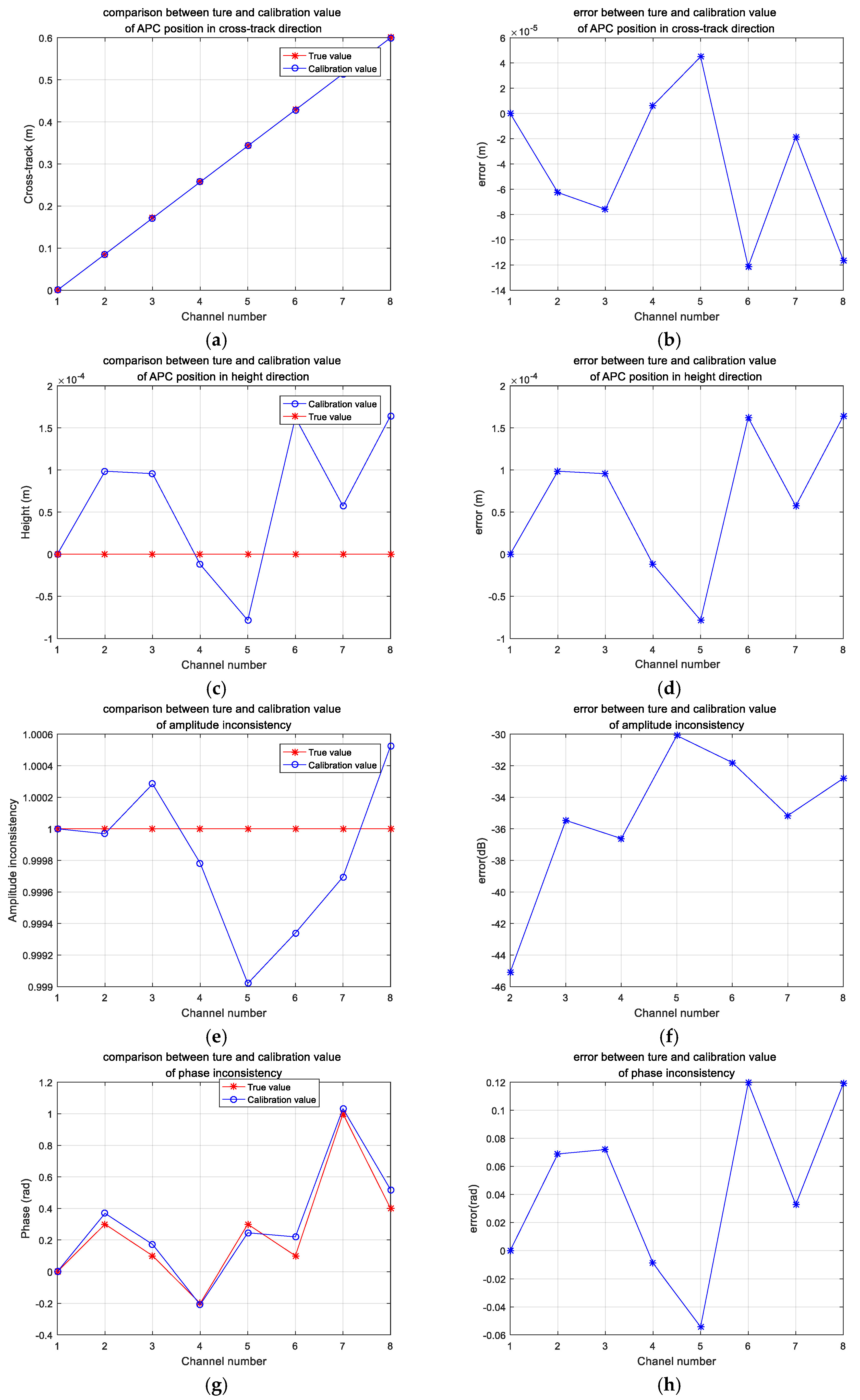
3.3. Validation with Simulation Data
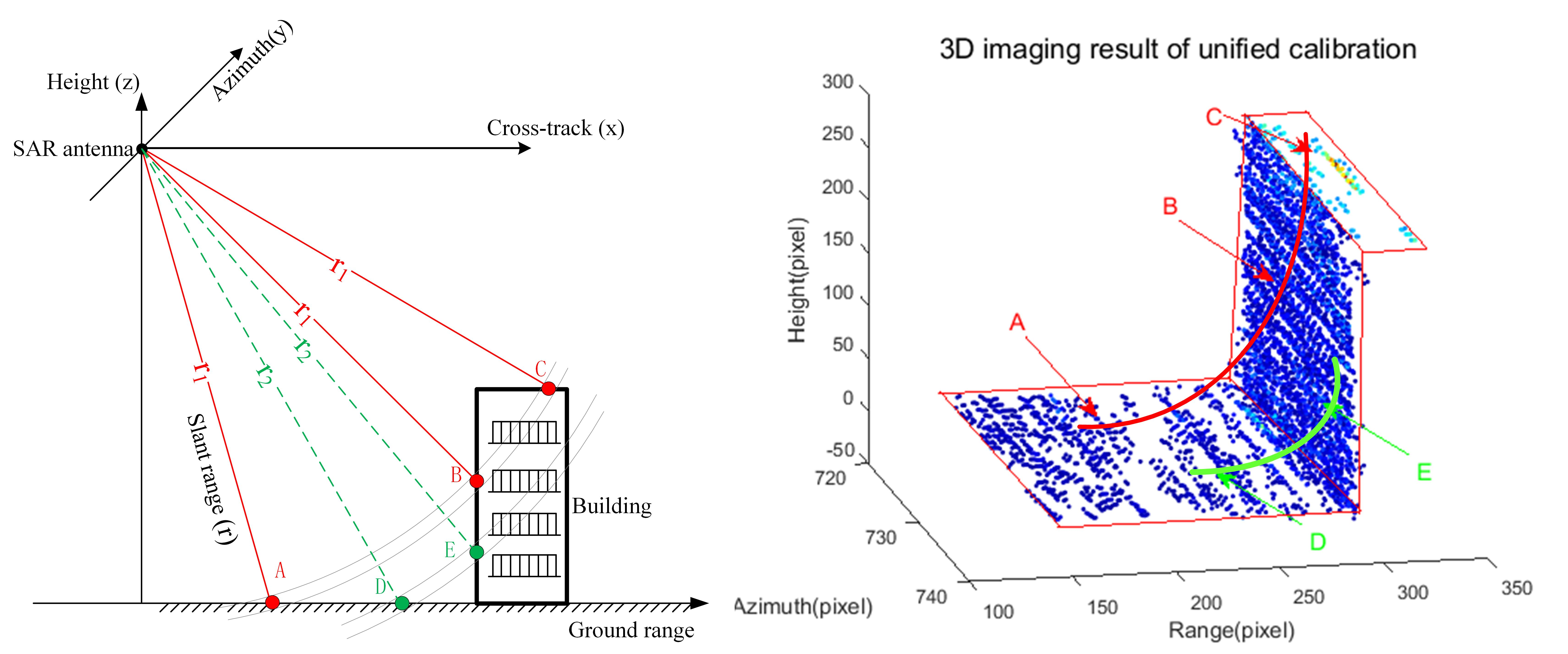
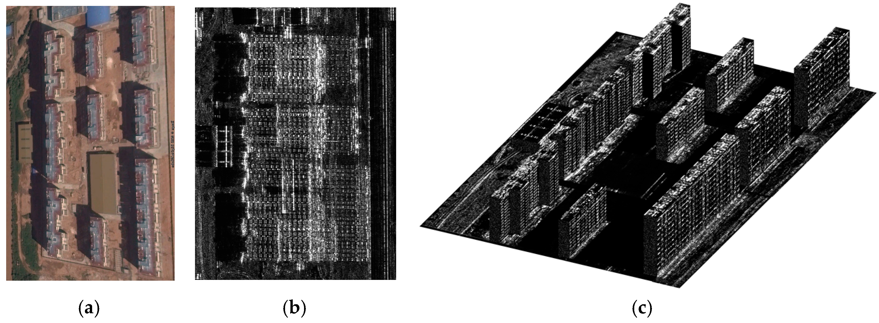
4. Experimental Results
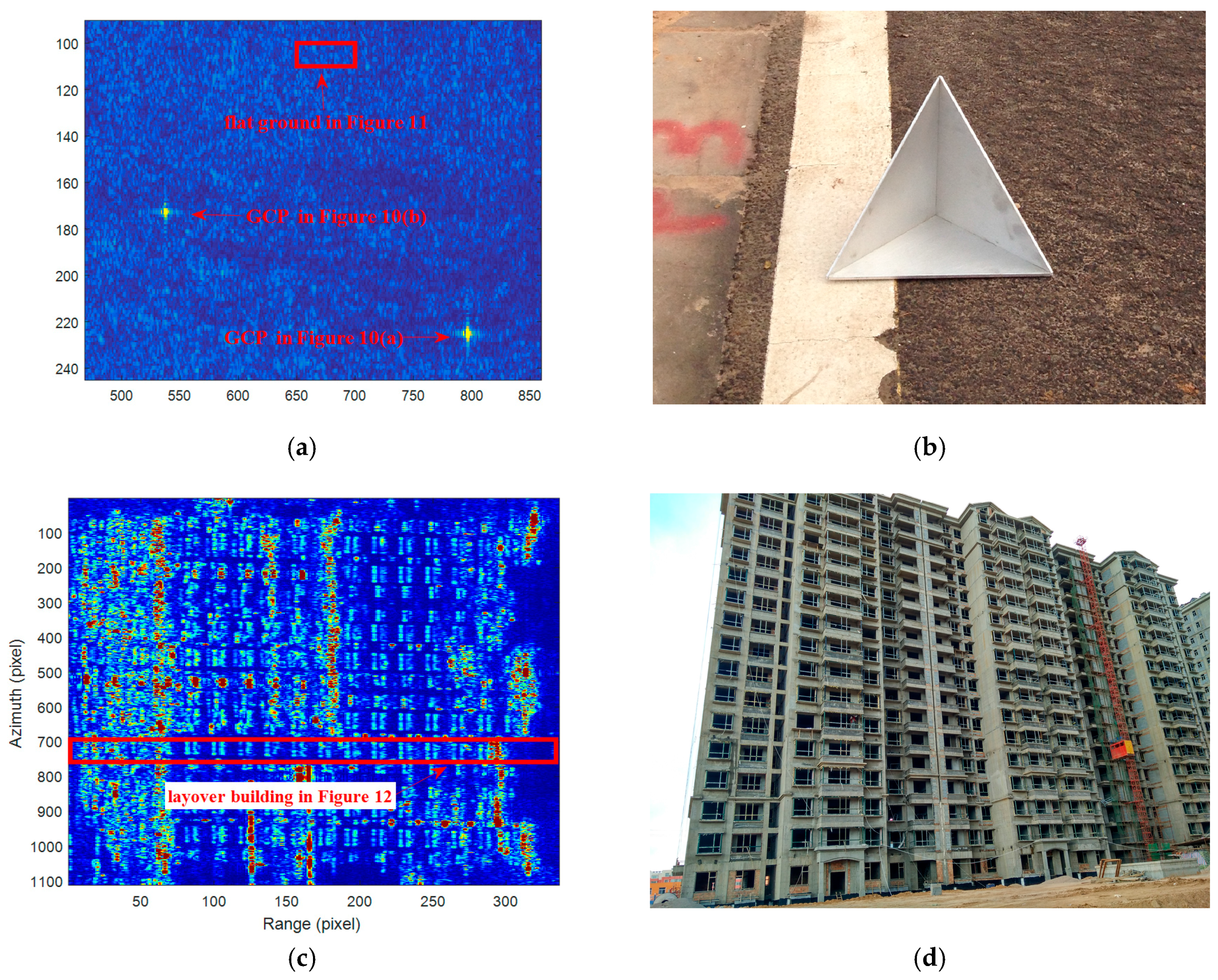
4.1. Data Acquisition
4.2. Validation Data Description
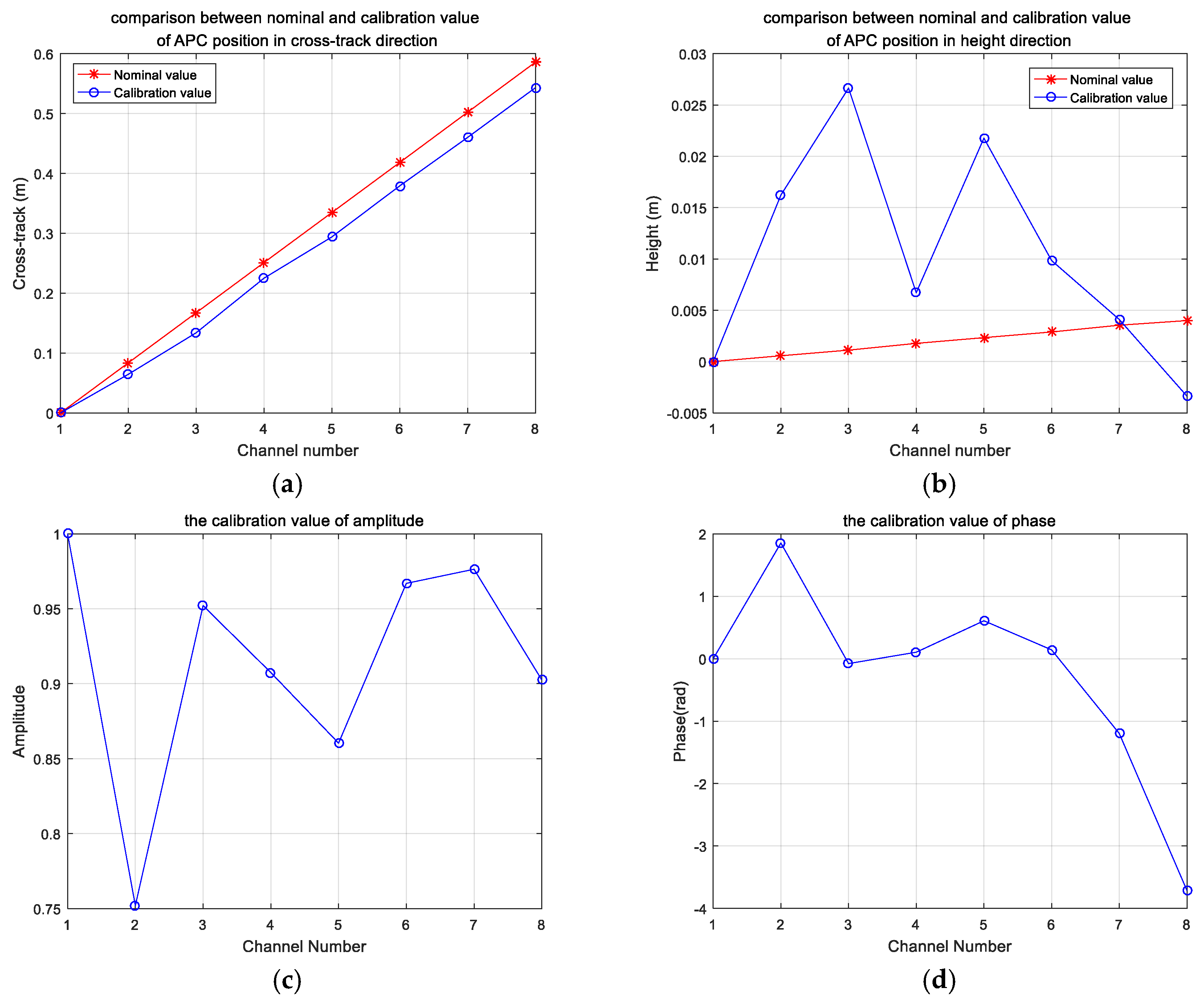
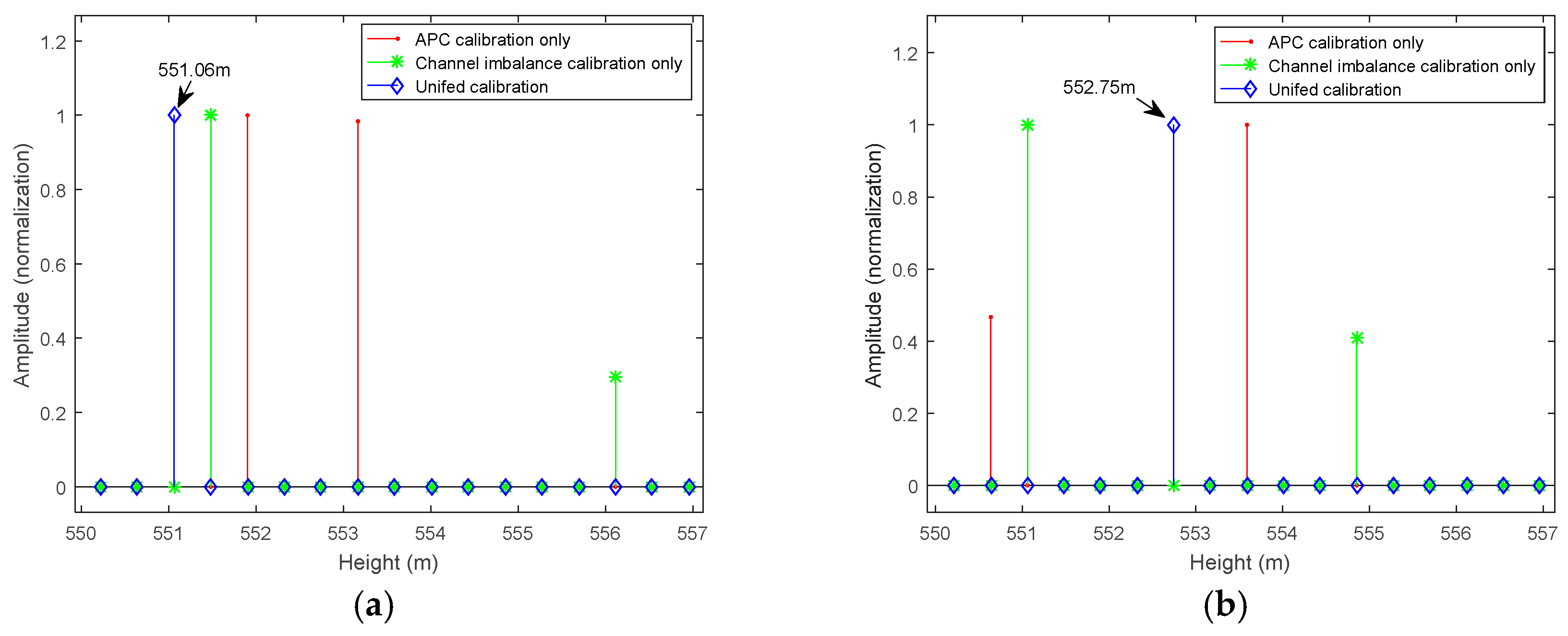
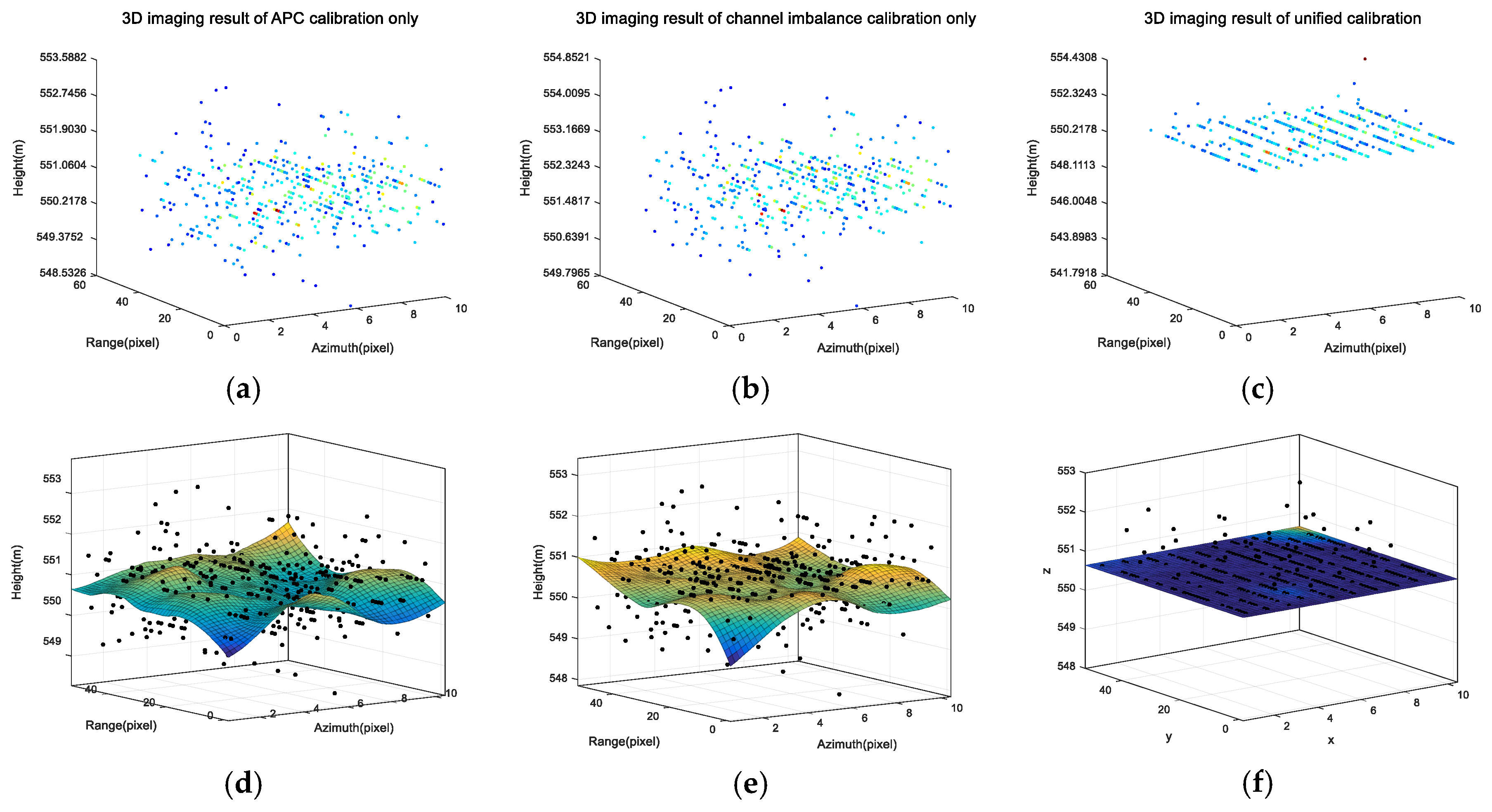
4.3. Calibration Algorithm Validation
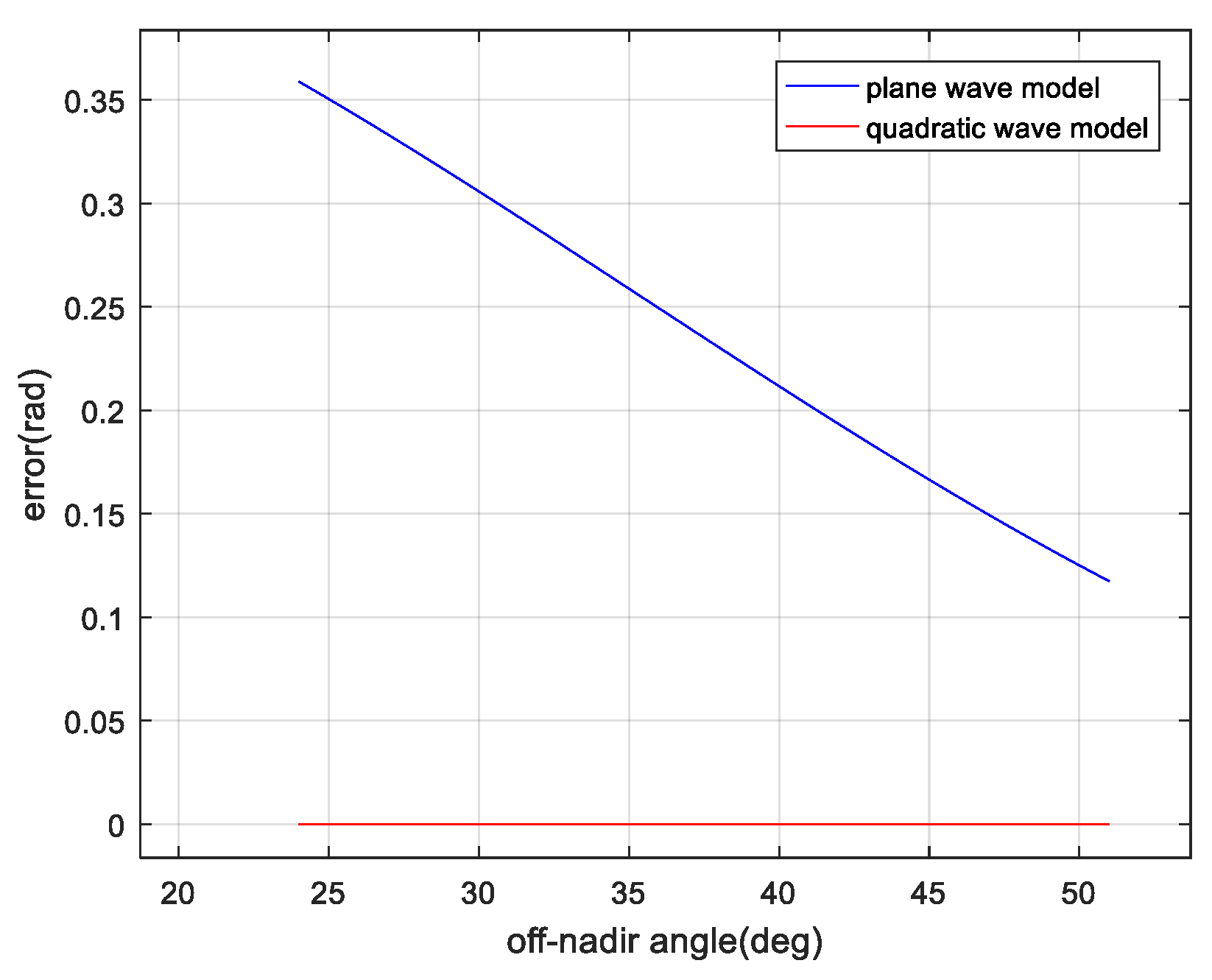
5. Discussion
6. Conclusions
Acknowledgments
Author Contributions
Conflicts of Interest
Appendix A
References
- Fornaro, G.; Lombardini, F.; Serafino, F. Three-dimensional multipass SAR focusing: Experiments with long-term spaceborne data. IEEE Trans. Geosci. Remote Sens. 2005, 43, 702–714. [Google Scholar] [CrossRef]
- Reigber, A.; Moreira, A. First demonstration of airborne SAR tomography using multibaseline L-band data. IEEE Trans. Geosci. Remote Sens. 2000, 38, 2142–2152. [Google Scholar] [CrossRef]
- Schmitt, M.; Stilla, U. Compressive sensing based layover separation in airborne single-pass multi-baseline InSAR data. IEEE Geosci. Remote Sens. Lett. 2013, 10, 313–317. [Google Scholar] [CrossRef]
- Zhu, X.X.; Bamler, R. Super-Resolution Power and Robustness of Compressive Sensing for Spectral Estimation With Application to Spaceborne Tomographic SAR. IEEE Trans. Geosci. Remote Sens. 2012, 50, 247–258. [Google Scholar] [CrossRef]
- Schmitt, M.; Stilla, U. Maximum-likelihood-based approach for single-pass synthetic aperture radar tomography over urban areas. IET Radar Sonar Navig. 2014, 8, 1145–1153. [Google Scholar] [CrossRef]
- Urasawa, F.; Yamada, H.; Yamaguchi, Y.; Sato, R. Fundamental study on multi-baseline SAR tomography by Pi-SAR-L2. In Proceedings of the URSI Asia-Pacific Radio Science Conference (URSI AP-RASC), Seoul, Korea, 21–25 August 2016; IEEE: Piscataway, NJ, USA, 2016; pp. 514–515. [Google Scholar]
- Frey, O.; Morsdorf, F.; Meier, E. Tomographic imaging of a forested area by airborne multi-baseline P-band SAR. Sensors 2008, 8, 5884–5896. [Google Scholar] [CrossRef] [PubMed] [Green Version]
- Schmitt, M.; Shahzad, M.; Zhu, X.X. Reconstruction of individual trees from multi-aspect TomoSAR data. Remote Sens. Environ. 2015, 165, 175–185. [Google Scholar] [CrossRef]
- Zhu, X.X.; Bamler, R. Superresolving SAR tomography for multidimensional imaging of urban areas: Compressive sensing-based TomoSAR inversion. IEEE Signal Process. Mag. 2014, 31, 51–58. [Google Scholar] [CrossRef]
- Zhu, X.X.; Bamler, R. Demonstration of Super-Resolution for Tomographic SAR Imaging in Urban Environment. IEEE Trans. Geosci. Remote Sens. 2012, 50, 3150–3157. [Google Scholar] [CrossRef] [Green Version]
- Tebaldini, S.; Rocca, F.; D’Alessandro, M.M.; Ferro-Famil, L. Phase Calibration of Airborne Tomographic SAR Data via Phase Center Double Localization. IEEE Trans. Geosci. Remote Sens. 2016, 54, 1775–1792. [Google Scholar] [CrossRef]
- Tebaldini, S.; Guarnieri, A.M. On the Role of Phase Stability in SAR Multibaseline Applications. IEEE Trans. Geosci. Remote Sens. 2010, 48, 2953–2966. [Google Scholar] [CrossRef]
- Pardini, M.; Papathanassiou, K.; Bianco, V.; Iodice, A. Phase calibration of multibaseline SAR data based on a minimum entropy criterion. In Proceedings of the Geoscience and Remote Sensing Symposium, Munich, Germany, 22–27 July 2012; pp. 1–4. [Google Scholar]
- Gocho, M.; Yamada, H.; Arii, M.; Sato, R.; Yamaguchi, Y.; Kojima, S. Verification of simple calibration method for multi-baseline SAR tomography. In Proceedings of the 2016 International Symposium on Antennas and Propagation (ISAP), Okinawa, Japan, 24–28 October 2016; IEEE: Piscataway, NJ, USA, 2016; pp. 312–313. [Google Scholar]
- Tebaldini, S.; Rocca, F.; D’Alessandro, M.M.; Ferro-Famil, L. Point-target free phase calibration of InSAR data stacks. In Proceedings of the 2016 IEEE International Geoscience and Remote Sensing Symposium, Beijing, China, 10–15 July 2016; pp. 1440–1443. [Google Scholar]
- Zhu, H. Study on Phase Center Calibration Methods of Linear Array Downward-Looking 3D-SAR. Master’s Thesis, University of Chinese Academy of Sciences, Beijing, China, 2012. [Google Scholar]
- Han, K. Study on Multi-Channel Amplitude-Phase Errors Calibration and Imaging Methods of Downward-Looking 3D-SAR Based on Array Antennas. Master’s Thesis, University of Chinese Academy of Sciences, Beijing, China, 2011. [Google Scholar]
- Yang, X.L.; Tan, W.X.; Qi, Y.L.; Wang, Y.P.; Hong, W. Amplitude and Phase Errors Correction for Array 3D SAR System Based on Single Prominent Point Like Target Echo Data. J. Radars 2014, 3, 409–418. [Google Scholar]
- Wang, Y. Studies on Calibration Model and Algorighm for Airborne Interferoemtric SAR. Ph.D. Thesis, University of Chinese Academy of Sciences, Beijing, China, 2003. [Google Scholar]
- Zhang, F. Research on Signal Processing of 3-D reconstruction in Linear Array Synthetic Aperture Radar Interferometry. Ph.D. Thesis, University of Chinese Academy of Sciences, Beijing, China, 2015. [Google Scholar]
- Li, H.; Ding, C.; Zhang, F.; Liang, X.; Wu, Y. A novel 3-D reconstruction approach based on group-sparsity of array InSAR. Sci. Sinica Inform. 2017. [Google Scholar] [CrossRef]
- Ng, B.C.; See, C.M.S. Sensor-array calibration using a maximum-likelihood approach. IEEE Trans. Antennas Propag. 1996, 44, 827–835. [Google Scholar]
- Rockah, Y.; Schultheiss, P.M. Array shape calibration using sources in unknown locations—Part I: Far-field sources. IEEE Trans. Acoust. Speech Signal Process. 1987, 35, 286–299. [Google Scholar] [CrossRef]
- Rockah, Y.; Schultheiss, P.M. Array shape calibration using sources in unknown locations—Part II: Near-field sources and estimator implementation. IEEE Trans. Acoust. Speech Signal Process. 1987, 35, 724–735. [Google Scholar] [CrossRef]


| Simulation Data Parameters | |
|---|---|
| Frequency | 15 GHz (Ku-Band) |
| Bandwidth | 500 MHz |
| PRF | 2000 Hz |
| Airplane altitude | 1000 m |
| Airplane Velocity | 60 m/s |
| Azimuth beam width | 2° |
| Depression angle | 25°–41° |
| Layover GCPs | Number of Targets | Height of Targets (m) | ||||
|---|---|---|---|---|---|---|
| True Value | Before Calibration | After Calibration | True Value | Before Calibration | After Calibration | |
| 1st pair | 2 | 3 | 2 | 0, 56.9 | 9.7, 138.2, 166.9 | 0, 56.9 |
| 2nd pair | 2 | 3 | 2 | 0, 32.7 | 0, 34, 143 | 0, 32.7 |
| 3rd pair | 2 | 3 | 2 | 0, 12.4 | 8.4, 34.9, 78.1 | 0, 12.4 |
| 4th pair | 2 | 4 | 2 | 0, 4.5 | 36, 126, 173.5, 176 | 0, 5.0 |
| Mean | Standard Deviation | |
|---|---|---|
| Amplitude (dB) | −35.10 | 4.15 |
| Phase (rad) | −0.0054 | 0.0577 |
© 2018 by the authors. Licensee MDPI, Basel, Switzerland. This article is an open access article distributed under the terms and conditions of the Creative Commons Attribution (CC BY) license (http://creativecommons.org/licenses/by/4.0/).
Share and Cite
Bu, Y.; Liang, X.; Wang, Y.; Zhang, F.; Li, Y. A Unified Algorithm for Channel Imbalance and Antenna Phase Center Position Calibration of a Single-Pass Multi-Baseline TomoSAR System. Remote Sens. 2018, 10, 456. https://doi.org/10.3390/rs10030456
Bu Y, Liang X, Wang Y, Zhang F, Li Y. A Unified Algorithm for Channel Imbalance and Antenna Phase Center Position Calibration of a Single-Pass Multi-Baseline TomoSAR System. Remote Sensing. 2018; 10(3):456. https://doi.org/10.3390/rs10030456
Chicago/Turabian StyleBu, Yuncheng, Xingdong Liang, Yu Wang, Fubo Zhang, and Yanlei Li. 2018. "A Unified Algorithm for Channel Imbalance and Antenna Phase Center Position Calibration of a Single-Pass Multi-Baseline TomoSAR System" Remote Sensing 10, no. 3: 456. https://doi.org/10.3390/rs10030456