Article

The Development of a Low-Cost, Near Infrared, High-Temperature Thermal Imaging System and Its Application to the Retrieval of Accurate Lava Lake Temperatures at Masaya Volcano, Nicaragua

by
Thomas Charles Wilkes
1,2,*,
Leigh Russell Stanger
2,
Jon Raffe Willmott
2,
Tom David Pering
1,
Andrew John Samuel McGonigle
1,3 and
Rebecca Anne England
1
1
Department of Geography, The University of Sheffield, Winter Street, Sheffield S10 2TN, UK
2
Department of Electronic and Electrical Engineering, The University of Sheffield, Portobello Centre, Pitt Street, Sheffield S1 4ET, UK
3
School of Geosciences, The University of Sydney, Sydney 2006, Australia
*
Author to whom correspondence should be addressed.
Remote Sens. 2018, 10(3), 450; https://doi.org/10.3390/rs10030450
Submission received: 29 January 2018 / Revised: 1 March 2018 / Accepted: 10 March 2018 / Published: 13 March 2018

Abstract

:
Near infrared thermal cameras can provide useful low-cost imaging systems for high temperature applications, as an alternative to ubiquitous mid-/long-wavelength infrared systems. Here, we present a new Raspberry Pi-based near infrared thermal camera for use at temperatures of ≈>500 °C. We discuss in detail the building of the optical system, calibration using a Sakuma-Hattori model and quantification of uncertainties in remote temperature retrievals. We then present results from the deployment of the system on Masaya Volcano, Nicaragua, where the active lava lake was imaged. Temperatures reached a maximum of 1104 ± 14 °C and the lake radiative power output was found to range between 30 and 45 MW. To the best of our knowledge, this is the first published ground-based data on the thermal characteristics of this relatively nascent lava lake, which became visible in late 2015.

Graphical Abstract

1. Introduction

Thermal imaging has applications across a wide range of fields, spanning a broad range of temperatures and thus, utilizing a number of different technologies and instruments. In volcanology, it can provide crucial information on the state of a volcanic system and can ultimately aid in monitoring efforts (e.g., [1,2]). Furthermore, thermal cameras are utilised by the scientific research community, to better understand a number of volcanic phenomena. For example, in some relatively early thermal imaging work, Oppenheimer and Yirgu [3] quantified the radiative power output from Erta ‘Ale’s lava lake, subsequently suggesting that crystallisation could be a significant driver of magma convection; in a multi-parametric study, including thermal and gas flux data, Peters et al. [4] found common cyclicities in a number of aspects of the behaviour of Erebus volcano and its active lava lake; on Stromboli, Delle Donne and Ripepe [5] used a relatively high frame-rate (50 Hz) thermal camera and differential pressure transducers to investigate Strombolian explosion dynamics and constrain their infrasonic source. More recently, with the increasing application of Unmanned Aerial Vehicles (UAVs) in volcanology (e.g., [6,7,8]), a lightweight thermal camera has been integrated into a UAV to map a geothermal field [9]. This allows relatively large areas (7000 m2 in this case) to be mapped, as well as enabling imaging to be performed over areas which are difficult or hazardous to access on the ground.
To date, volcanic applications have predominantly involved commercial thermal cameras [1]. These systems use sensors with good responsivity within one of two atmospheric windows, 3–5 μm (Mid-Wavelength InfraRed; MWIR) or 8–14 μm (Long-Wavelength InfraRed; LWIR) and are generally rather expensive ($1000 s–$10,000 s). They are commonly used in scientific, industrial and military applications and, unlike consumer electronics, have not been exposed to intense market competition; thus, costs remain high and product cycles are relatively long. Recently, however, a few studies have made use of consumer visible imaging systems to develop low-cost, portable thermal cameras for imaging relatively high temperature (>300 °C) objects [10,11,12]. Unlike the aforementioned scientific thermal cameras, these systems use silicon semiconductor detectors, which are sensitive to wavelengths ≈≤ 1.1 μm and, therefore, provide some sensitivity in the Near InfraRed (NIR).
Since this article focuses on the development of a NIR consumer electronics-based thermal camera, here, it is important to briefly discuss both the strengths and weaknesses of thermal cameras working at these shorter wavelengths. Firstly, according to Planck’s law, as temperature reduces, the peak of a radiating body’s radiant exitance moves toward longer wavelengths and the total energy emitted decreases; thus, thermal cameras that are sensitive only to shorter wavelengths will be limited solely to applications imaging hotter objects. Such cameras are, therefore, only suitable for volcanological applications involving temperatures some hundreds of degrees Celsius above ambient. Secondly, due to increasing solar irradiance, moving from LWIR to NIR wavelengths, daytime acquisitions will be more strongly affected by reflected sunlight when using short wavelength detectors. However, an advantage to imaging at shorter wavelengths is that there is significantly less absorption by atmospheric H2O and CO2 relative to the MWIR/LWIR (e.g., [11,12]), even within the two atmospheric windows mentioned above. This becomes increasingly important for temperature calibration when measuring through long atmospheric path lengths, or through potentially concentrated gases such as in volcanic plumes; however, the scattering from aerosols may be more significant at these shorter wavelengths. Dixon [13] used Planck’s equation to show that for a certain instrument precision, the measurement error decreases with decreasing wavelength and, thus, NIR detectors have the potential to provide more precise temperature measurements, if all else remains equal. MWIR/LWIR cameras also generally have quite low spatial resolutions, relative to visible-NIR detectors, which can lead to significant errors in accurate temperature determination (e.g., [14]). It should be noted, however, that these technologies are improving and reducing in cost, albeit at a slower pace than in the case of consumer electronics.
To date, previous uses of low-cost consumer imaging systems have had some drawbacks, predominantly due to the limited user control of the sensor, or due to the calibration procedures. For example, an early attempt at this work by Saito et al. [10] was limited by the camera’s automatic shutter speed and gain control, which resulted in small hot objects saturating the sensor if the rest of the scene was notably cooler. Also, automatic post-processing of image frames can introduce sensor non-linearity, with respect to incident radiation, which must then be corrected for; however, it is not clear the extent of error, if any, introduced during this correction. Furukawa [11] used a Canon EOS 300D camera, which gave much greater user control. Their calibration scheme of heating rock in a furnace may be quite accurate, however, if the experimental setup is not extremely rigorous, in order to ensure that the sample is a freely radiating surface, significant errors could be incorporated into this technique.
Most recently, a low-cost thermal imaging system has been proposed by Radebaugh et al. [12], using the Raspberry Pi camera module (referred to as PiCam hereafter) and an absolute photometric calibration scheme involving reflective card; however, notable limitations in the calibration procedure are highlighted therein. Although this may provide a relatively simple, inexpensive means of investigating temperature changes, the use of the PiCam’s video port, which prevents fixing of the sensor’s gains, may well introduce significant errors into the data, as acknowledged by the authors. Gain amplifies the sensor signal and, thus, the calibration (i.e., mapping of signal to temperature) becomes obsolete if the gain changes after calibration, unless a correction for this effect is applied (e.g., [10]). Furthermore, since the value of gamma was only estimated, reversing the gamma correction may also have incorporated errors. Conversely, in previous work, which is corroborated herein, we have shown the RAW sensor data extracted from the PiCam module to have a linear relationship to radiance, since it negates any post-processing effects present in the JPEG frames [15]. Furthermore, the RAW images provide 10-bit digitisation (1024 digital levels), whilst all other presented work with low-cost NIR thermal cameras have utilised 8-bit images (256 digital levels) which dramatically limits the temperature range and precision over which the instrument can measure. It should be noted that the instruments used in previous work have been capable of producing higher bit-depth images, however, this option was not exploited.
Finally, the quantum efficiency of visible imaging cameras in the NIR band can be somewhat limited due to the Bayer filter mosaic, which overlies the silicon focal plane array. If the RAW sensor data is extracted, this filter also produces a non-uniform pixel response, creating a mosaic pattern, which is undesirable in thermal imaging applications (e.g., [15,16]). Through removal of the Bayer filter, following [15], we eliminate the mosaicking complication whilst also producing a sensor with heightened sensitivity in the NIR.
In this article, we therefore present what we believe to be a more precise and accurate PiCam NIR thermal camera, which benefits from 10-bit RAW output, fixed analogue gain and a blackbody furnace calibration. The utility of this smartphone sensor-based camera board has already been highlighted in a number of studies (e.g., [12,15,17,18,19]), facilitating the development of low-cost alternatives to previously expensive technologies. We also quantify and discuss a number of uncertainties in this measurement technique, to emphasise the issues faced when attempting to retrieve absolute temperatures remotely. The system was deployed and tested on Masaya volcano, Nicaragua, where an active lava lake was imaged. A recent article by Aiuppa et al. [20] provides a detailed investigation into Masaya’s recent phase of activity (2015–2017), using ground-based gas data and satellite thermal data retrievals; however, the thermal data is limited by its relatively coarse resolution (1 km) and low temporal resolution (4 returns per day). Therefore, in addition to the aforementioned novelties of this study, to the best of our knowledge this article is also the first detailed report of ground-based temperatures from Masaya volcano since the new lake appeared in late 2015 [20,21].

2. Materials and Methods

2.1. Instrumental Design

The thermal imaging PiCam developed here is based on the Raspberry Pi camera module (v1.3), with the integrated Omnivision OV5467 sensor modified as described in Wilkes et al. [15]. As discussed in Section 1, this procedure, which involves removal of the Bayer filter, produces a uniform sensor with heightened sensitivity at both ultraviolet and near infrared wavelengths; the latter spectral band is pertinent to this work.
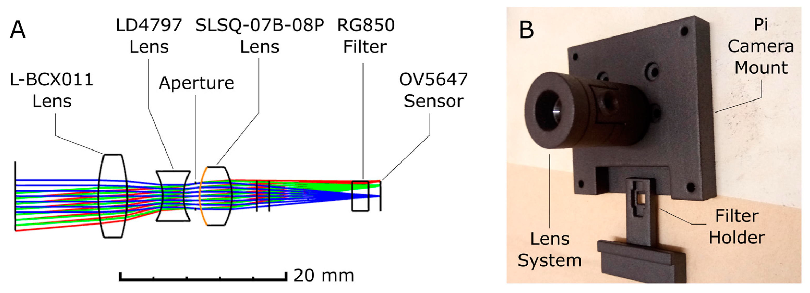
An optical system, shown in Figure 1A, was designed in OpticStudio (Zemax Ltd., Kirkland, WA, USA), to provide a 10° field of view (FOV) for the camera; this FOV had been determined to be appropriate based on estimates of the viewing geometry (Figure 2) and Masaya’s lava lake size provided by Instituto Nicaragüense de Estudios Territoriales (INETER; Personal Communication, 2017). The lens configuration was a triplet comprising off-the-shelf lenses (Ross Optical, L-BCX011; Thorlabs, LD4797; Optosigma, SLSQ-07B-08P), with a long-pass 850 nm filter (Thorlabs, RG850) positioned behind this lens system; a metal aperture of 3 mm diameter was located between the LD4797 and SLSQ-07B-08P lenses. A lens holder was then designed in SolidWorks and 3D printed with selective laser sintering (3dprintdirect.co.uk), to house the optical system and mount it to the camera board (Figure 1B).
The camera module was controlled by a Raspberry Pi 3 Model B computer (www.raspberrypi.org/), which in turn was controlled by a laptop connected wirelessly by the use of the Pi 3’s built in wireless hotspot capabilities. A Python3-based graphical user interface, developed in-house, was used to communicate with the Raspberry Pi and camera module and receive images from the Pi to be displayed on the laptop in real-time. For all work discussed herein, images were converted to temperatures post-acquisition and, thus, there was no real-time display of retrieved temperatures.
The Python package picamera allows relatively comprehensive control of the Pi Camera module. Analog gain was fixed at 1 and an optimal shutter speed, which gave a maximum pixel saturation in an image of approximately 80%, was then found experimentally; greater levels of saturation should be avoided, since sensors can begin to respond non-linearly as they approach saturation. These steps ensure a high signal-to-noise ratio (SNR) for each image. As discussed in Section 2.4, we find our calibration fits well to a square root dependence on signal. This indicates that the system is shot noise limited and, thus, SNR will increase proportionally to t1/2, where t is the integration time (i.e., shutter speed). Pixels were also software-binned from the full resolution 2592 × 1944 to 648 × 486, to further increase SNR, and saved in this smaller format. It could be argued here, however, that maintaining the high pixel resolution would be advantageous for retrieving accurate temperatures, especially when imaging small features which are sub-pixel scale in the 648 × 486 images. In such a scenario, the high resolution of this sensor (5 mega-pixels), relative to commercial MWIR/LWIR thermal cameras, could prove highly beneficial for accurate determination of small feature temperatures (e.g., [14]).

2.2. Calibration Procedure

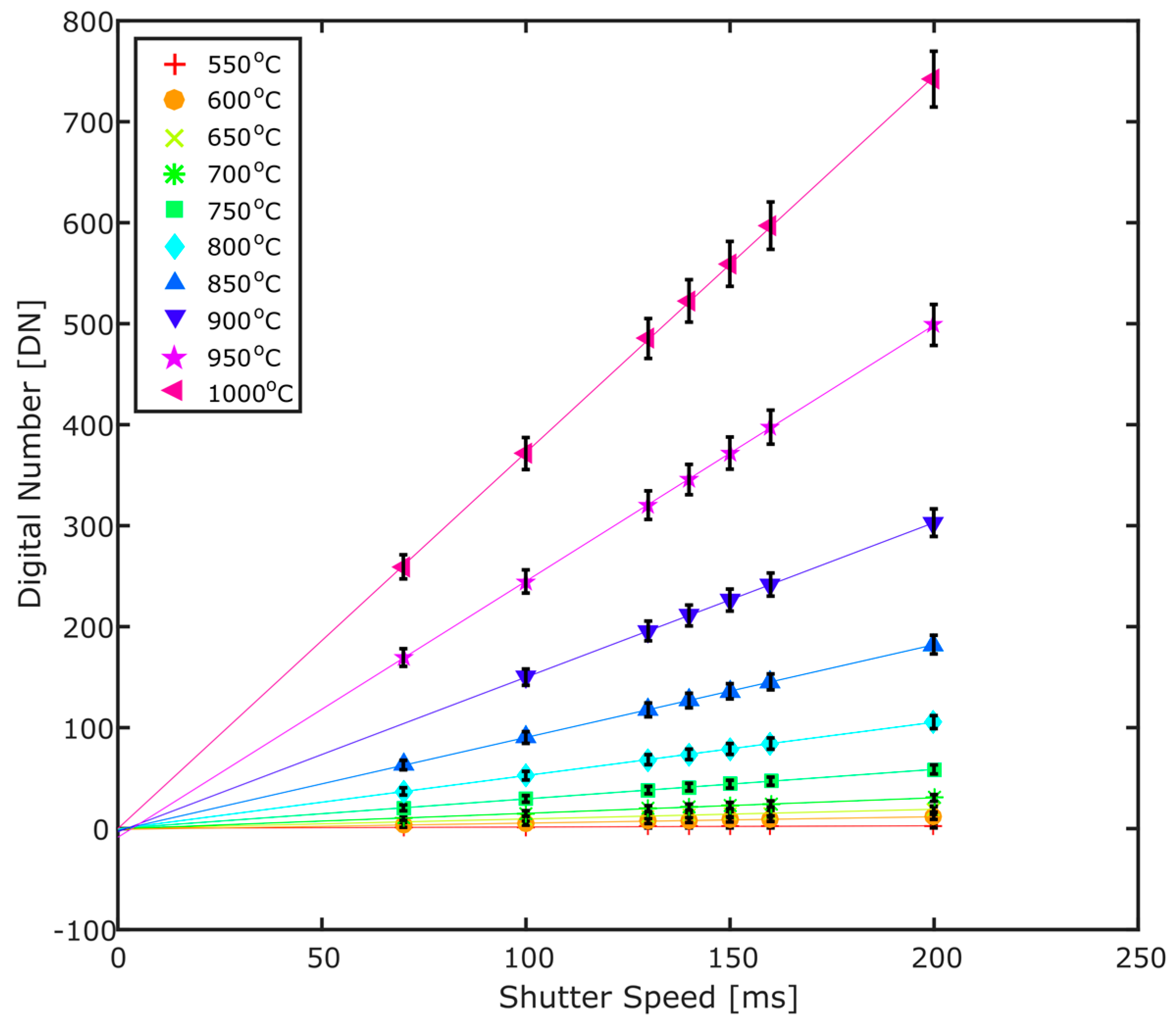
The camera was calibrated using a blackbody furnace (Landcal P1200B), with a thermocouple providing UKAS [www.ukas.com] certified temperature measurements of the source. The effective emissivity of the furnace is quoted as 0.998 if its cavity is isothermal. Images were then taken of the source at temperatures between 500 and 1000 °C, in 50 °C increments, and at a number of shutter speeds. For each temperature/shutter speed 30 images were taken and pixel Digital Numbers (DNs) were averaged in both the spatial and temporal domain, to provide a single DN representative of that temperature/shutter speed. To improve the calibration, the upper end of the temperature range could be increased, to extend the calibration beyond the maximum temperature expected from the lava lake. Issues with the furnace prevented capturing the whole range of lake temperatures (maximum of ≈1100 °C) in our calibration here; however, the calibration fit is extremely strong, with a standard error of 1.08 °C (see Table 1 and Table A1) and, thus, we are confident of the retrieved temperatures even when extrapolating beyond the 1000 °C. Although here we perform a single calibration to be applied to all pixels across an image, it is possible to perform the calibration for each pixel individually, which can account for non-uniform pixel sensitivity (e.g., [22]).
The recorded signals, S m e a s (discussed as the DN herein), at the given temperatures in Kelvin, T K , were fitted to the Planckian form of the Sakuma-Hattori equation (e.g., [23]) with 3 fitting coefficients, A0, A1, A2:
S m e a s ε β S S H = ε β A 0 exp ( c 2 A 1 T K + A 2 ) 1
where ε is the surface emissivity, β is the path transmission coefficient and c 2 is the second radiation constant (1.43877736 × 10⁻²). Results of this fit are displayed in Appendix B. Inversely, with known fitting parameters and for a given signal, temperature can be retrieved with:
T K c 2 A 1 l n ( ε β A 0 S m e a s + 1 ) A 2 A 1
Finally, we can differentiate Equation (1), producing a derivative which is utilised in the uncertainty analysis in Section 2.4.
S m e a s T = ε β S S H T = ε β [ S ( T K ) ] 2 A 1 c 2 A 0 ( A 1 T K + A 2 ) 2 e x p ( c 2 A 1 T K + A 2 )
In view of later discussion, we note here that since S m e a s ( T ) is monotonic, S m e a s T 1 = ( S m e a s T ) 1 .
Two methods of calibration were attempted. In the first, Sakuma-Hattori fit coefficients were determined individually for each shutter speed, i.e., calibration with the furnace was performed for a small set of known shutter speeds; thus, we generate fit coefficients A0, A1, A2 specific to a single shutter speed. Although the sensor response is linear with changing shutter speed, as demonstrated by Wilkes et al. [15] and confirmed here with the blackbody furnace (Appendix C), we performed a separate calibration for each specific shutter speed used throughout the campaign, to ensure integrity of results. This method can be time consuming, especially if a large number of different shutter speeds are used in field deployment. In the second method, the sensor response was assumed to be perfectly linear in DN vs. radiance and passing through the origin; thus, a single set of fit parameters were determined for a shutter speed of 1 μs and all signals were scaled to a 1 μs signal by dividing by the shutter speed of that acquisition. This technique depends on perfectly linear response of the sensor and an accurate dark current/offset correction; however, as can be seen from the calibration data (Appendix C), dark current subtractions do not always perfectly account for the offset in an image, for reasons which are unclear. Hence, although we see an extremely linear response of the sensor to incident radiation with increasing shutter speed, a perfect calibration, which covers all shutter speeds is difficult to establish. Furthermore, Lane and Whitenton [22] recommend cross-checking calibration points which have been scaled for varying integration times, acknowledging the difficulty of providing one calibration to fit all sensor integration times. The results presented here are therefore only based on the first method of calibration.

2.3. Extinction and Emissivity

From Equation (1), it can be seen that in order to retrieve accurate temperature measurements from our NIR thermal images, two final parameters need to be considered: the extinction of radiation between the object and the observer and the emissivity of the object. Both can have significant effects on the apparent temperatures observed by the instrument.
Atmospheric extinction comes in two forms, absorption and scattering of radiation by particles between the emitting object and the measuring instrument. Neglecting re-emission of radiation, extinction and transmission must sum to unity and, thus, understanding extinction can allow us to calculate β in Equation (2). Arguably, scattering due to aerosols is a significantly more complex radiative transfer problem than absorption. If imaging through an optically thick plume can be avoided this is preferential, otherwise, retrieving accurate temperatures would be extremely difficult and beyond the scope of this paper. If the aerosol loading is relatively stable with time, temperature measurements may still be able to provide useful insights into changing lake dynamics, without providing accurate absolute temperatures. Conditions where no plume condensation occurs are always preferable; nevertheless, in cases where aerosol is an issue, MWIR/LWIR cameras may perform better than a NIR alternative (e.g., [2]). Conversely, with regards to extinction through absorption, the NIR system is possibly less affected than a MWIR/LWIR system (e.g., [11,12]). Sawyer and Burton [24] addressed this issue well for MWIR/LWIR imaging, whilst Radebaugh et al. [12] give a good discussion for the NIR application. However, the latter only discuss this issue and do not correct their temperatures for absorption. Here, we estimate the amount of absorption across the viewing path and subsequently correct our temperatures for this effect.
Within the spectral sensitivity band of our instrument (≈850–1100 nm), only H2O exhibits significant absorption, therefore simplifying the absorption correction to this single gas species. Furthermore, attenuation due to absorption is relatively straightforward to quantify, since high resolution absorption/transmission spectra for most, if not all, common gaseous species are openly available via the High Resolution Transmission database (HITRAN; [25]). Using the bytran software [26], which utilises the HITRAN Application Programming Interface (HAPI; [27]) to extract and manipulate molecular line intensities, we generated data for transmission vs. wavelength. Relative humidity (RH) and temperature data, logged during the Masaya field campaign, and an estimated atmospheric pressure were then used to scale the transmission spectrum according to the column density of water in the instrument’s line-of-site. The two extremes of measured conditions, 26.5 °C and 82% RH and 31.9 °C and 60% RH, were used in these calculations, assuming that conditions do not change across the viewing path; in reality, this assumption will not be perfect, since conditions close to the lava lake surface are likely to be significantly different from our measurements made on the crater rim. Using these spectra, along with the spectral response of the PiCam with the long-pass filter in place (determined using a monochromator), we determined the effect on observed temperature by integrating Planck’s equation with these two filter spectra applied. The ratio of this calculated signal to the signal without the H2O spectrum filter provides a path transmission coefficient, β , which can be directly used in Equation (2) during temperature retrievals. If all atmospheric parameters remained constant, the path transmission coefficient would still be a non-constant scalar, since it is dependent on the temperature of the emitting body. This is because the shape of the blackbody curve varies with temperature and, therefore, the proportion of absorption from each H2O absorption line changes with this changing distribution of spectral radiance. Since the majority of, if not all, lava lake temperatures range between 800–1200 °C (see Section 3), we calculate the transmission coefficients between these temperatures, in 100 °C increments and take an average. We therefore have a single β , averaged across both temparature and atmospheric conditions, which can be used in temperature retrievals; for this work, β = 0.8789 . In Section 2.4 we quantify the uncertainty associated with using this single transmission coefficient for the Masaya lava lake dataset.
The water absorption effect could be almost entirely removed by using a second optical filter to attenuate radiation around the absorption peak at ≈940 nm. Rudimentary tests of this were attempted in the field using band-pass filters, centred at 850 and 1080 nm (10 nm full-width-at-half-maximum; Knight Optical), mounted to the fore of the lens system. Due to this optical setup, however, images appear to display some vignetting/aberrations. Furthermore, longer shutter speeds (100–200 ms) were required in order to obtain greater signal, due to the decrease in radiation incident upon the sensor caused by the filters. Since Masaya’s lava lake was moving extremely rapidly, this caused some blurring of the image scene. In cases of extremely humid conditions or long path lengths, or where the scene is relatively stationary, an additional filter could be advantageous. Here, however, we discuss only data acquired using the single long-pass 850 nm filter.
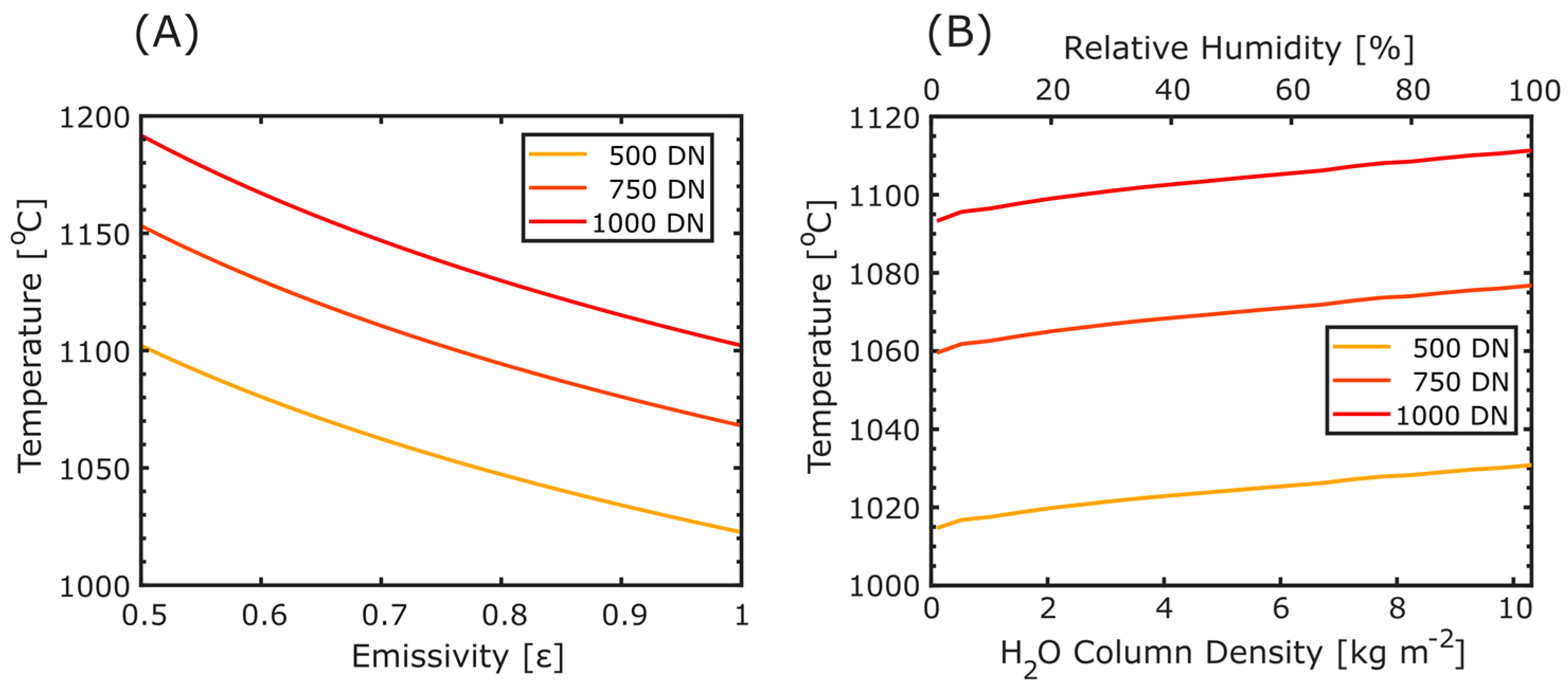
In the literature, hitherto, a range of emissivities (≈0.5–1.0) have been used for basalts within the wavelength range of 0.8–1.1 μm ([28] and references therein). Nevertheless, at a signal DN of 750, assuming an emissivity of 1 only underestimates the temperature by ≈12 °C if the actual emissivity were 0.9 (Figure 3A); this emissivity is also very much at the lower end of most estimates, if excluding the broad range (0.5–0.9) presented by Rothery et al. [29] where emissivity was not directly measured, rather, it was inferred from Kirchoff’s law and reflectance determined through satellite imagery. Ideally, for each application, a rock sample would be taken from the field and its emissivity measured; however, if this experiment is not conducted in a rigorous manner, to obtain a freely radiating surface, significant errors can be incorporated into this calculation. We therefore, somewhat arbitrarily, assume an emissivity of 0.95 and acknowledge that this will affect the absolute temperatures presented herein. Due to the paucity of emissivity data in the NIR, we then assume a bounding range of 0.9–1.0, with a uniform distribution, to calculate σ ε (Equation (10)) for the uncertainty analysis in Section 2.4.
The emissivity of an object is a function of a number of parameters, including: chemical composition, surface roughness, viewing angle and porosity. When the lava lake is in a relatively non-turbulent state, it may be reasonable to assume that the change in emissivity is relatively small. Under such conditions erroneous estimation of this parameter will only cause over- or under-estimation of the absolute temperature by a constant value during an acquisition sequence; however, between states of turbulence and relative stability, emissivity may vary, making such an assumption less valid. Similarly, atmospheric conditions, volcanic gas emissions and the mixing ratio of the two, can vary quite considerably over relatively short time periods and, thus, could result in a variable path transmission coefficient. Were this variation significant, it would not only affect the absolute calibration of the instrument but could also mask/influence any trends or periodicities in a temperature time series; this latter effect may be more problematic, since it is likely that volcanologists are more concerned with thermal signatures which can relate to changes in volcanic activity (e.g., [1,2,30]), rather than a perfect radiometric calibration of temperature. As part of the following section we show that, for conditions experienced on Masaya, the uncertainty caused by a variable path transmission coefficient is negligible for this PiCam instrument.

2.4. Uncertainty Analysis

A number of uncertainties can be quantified with respect to the final quoted temperatures. Quite often these are neglected or poorly constrained within the field of volcano remote sensing, however, it is important to understand these constraints when evaluating datasets. We therefore give a detailed discussion of our uncertainty analysis herein. We will discuss each uncertainty separately, as they are considered independent and can, therefore, be added in quadrature to provide a total uncertainty estimate of a retrieved temperature. Lane et al. [31] provide a comprehensive overview of much of the work presented in this section.
The calibration uncertainty consists of four sources (Table 1). These uncertainties are, again, assumed uncorrelated and, thus, added in quadrature to provide a total calibration uncertainty ( σ c a l ). In this case, we multiply the total by a factor of 2 to provide a 95% confidence interval:
Δ T c a l = 2 σ c a l = 2 σ T c B B 2 + σ T B B 2 + σ ε B B 2 + σ f i t 2
It can be seen that this uncertainty is temperature dependent due to the temperature dependence of the blackbody furnace’s emissivity uncertainty. Therefore, this standard uncertainty can be plotted against temperature and a linear regression is performed to estimate Δ T c a l given any temperature, T :
Δ T c a l ( T ) = B 0 + B 1 × T K
The measurement noise is specific to the camera sensor. In an optical system which is performing optimally this will be dominated by shot noise, which has a square root dependence on signal:
σ n o i s e = C 0 S m e a s + C 1
where, in this case, the fit coefficients C 0 and C 1 were empirically determined to be 0.109768 and 0.15447, respectively. This can be converted to a temperature uncertainty, again at 95% confidence level, using:
Δ T n o i s e = 2 σ n o i s e × S T 1
In this study, we do not employ any flat-field (i.e., uniform pixel illumination) correction, which can account for variation in pixel-to-pixel sensitivity, vignetting and other optical effects, and dust or scratches on the sensor. By imaging a homogenous surface, or clear sky at dusk or dawn, variations across the field of the camera can be accounted for; thus, it should be possible to totally remove, or at least make negligible, this uncertainty. Instead, here we quantify this uncertainty as another contributor to the overall uncertainty estimate. An image was taken of a flat reflecting object and the standard deviation of signal across the sensor was determined. The fraction of this standard deviation relative to the mean signal across the sensor can then be used to quantify the flat-field related temperature uncertainty, σ f l a t , as follows:
Δ T f l a t = 2 σ f l a t = 2 × S D f × S m e a s × S T 1
where Δ T f l a t is the temperature uncertainty at 95% confidence level and S D f = 0.03 is the empirically derived fractional standard deviation across the sensor. It should be noted that this flat-field image will also contain other associated sensor noise components, such as shot noise. To remove this uncertainty from the image we average a sequence of 30 images, on a pixel-by-pixel basis, making the contribution from this noise source negligible. The uncertainty associated with random sensor noise is equal to σ N where N is the sample size and σ is the standard deviation. Therefore, it is important to use enough images to make this uncertainty negligible; we found that 30 images were adequate here. The standard deviation of the resulting image is therefore almost entirely due to deviation from a perfect flat-field setup.
The total temperature uncertainty is now calculated by adding all considered uncertainties in quadrature:
Δ T t o t a l 2 = Δ T c a l 2 ( T ) + Δ T n o i s e 2 ( S m e a s ) + Δ T f l a t 2 ( S m e a s ) + Δ T x 2
where Δ T x 2 represents the sum of the squares of any further uncertainties which may not be directly associated with the PiCam instrument or calibration. In our case, we further estimate transmission coefficient and emissivity uncertainties, following from the discussion in Section 2.3.
There are two uncertainties associated with the transmission coefficient β . The first uncertainty pertains to atmospheric variability. For simplicity, we assume that the extreme values of atmospheric conditions stated in Section 2.3 provide the bounds for a uniform distribution function of the path transmission coefficient. The standard deviation, σ β , can then be calculated by the general equation:
σ x =   1 12 ( x m a x x m i n ) 2
where x m i n and x m a x are the lower and upper limits of a variable, x , respectively; in this case this is the path transmission coefficient β .
There is also a transmission coefficient uncertainty associated with object temperature (see Section 2.3). Using the extremes of temperatures to calculate two transmission coefficients, again we use Equation (10) to find the standard deviation of β with respect to temperature changes. The final transmission coefficient, therefore, incorporates uncertainties related to both atmospheric conditions and the temperature of the emitting object. These are independent of each other and are, therefore, added in quadrature to be incorporated into the final uncertainty. We do not include extinction through scattering in our quantification of uncertainties, since it is difficult to constrain; however, we acknowledge and later show (see Section 3), that it can have a significant impact on measurements.
The uncertainty of β can now be calculated using the general equation:
Δ T x = Δ x × Y × S S H × ( S m e a s T ) 1
where Δ x = 2 σ x for the uncertainty at 95% confidence level of variable x , which is in this case β ; Y is then the product of any further scaling factors from Equation (1), which in this case is simply the emissivity, ε .
As stated in the previous section, emissivity was also assumed to have a uniform distribution, between 0.9 and 1.0, due to the paucity of data on this parameter; furthermore, its high dependence on composition suggests that drawing values from articles at different volcanoes may be somewhat fallible. Again, the standard deviation, σ ε , is defined by Equation (10) and the standard uncertainty, Δ T ε , is calculated from Equation (11), where Y is now the path transmission coefficient β .
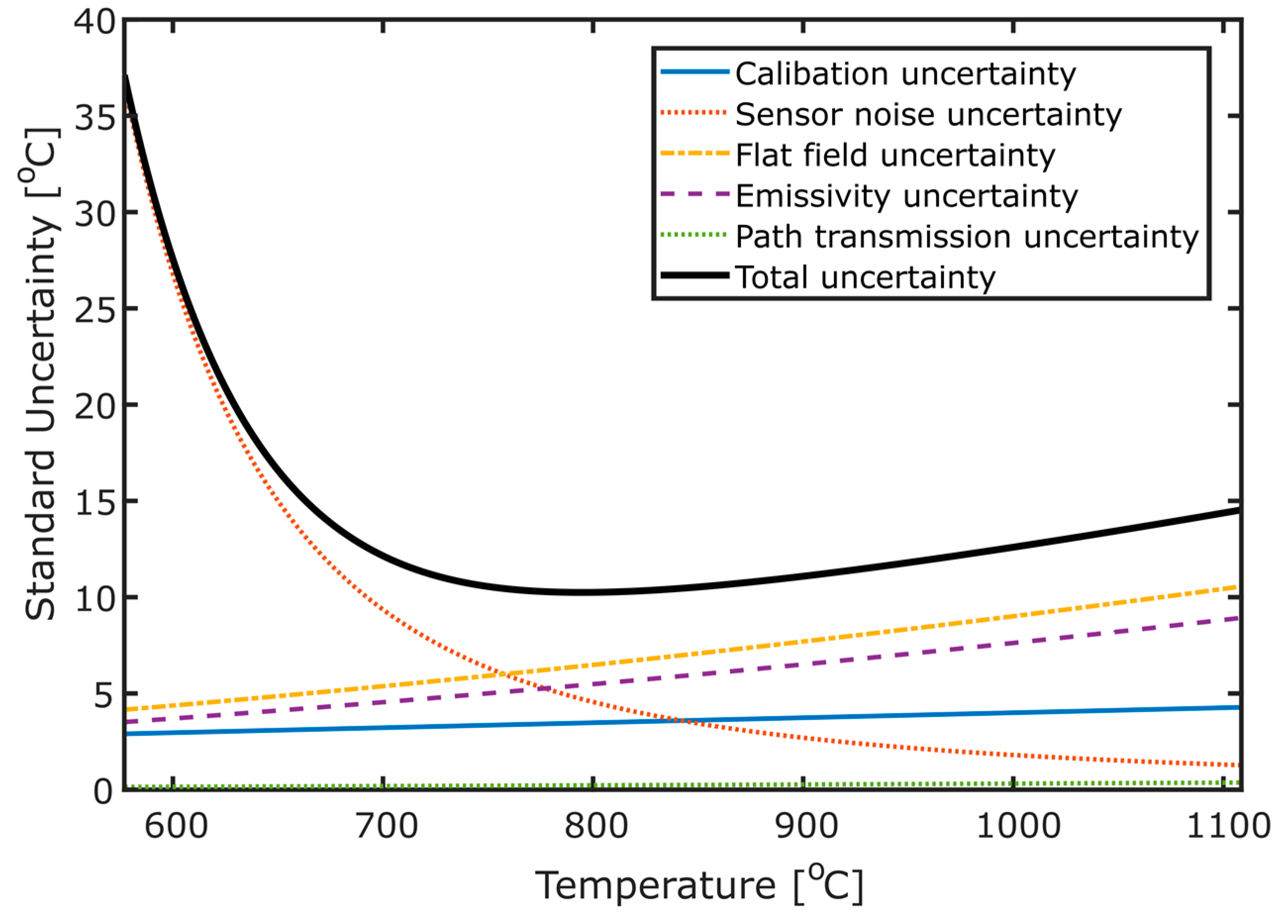
All uncertainties have a signal or temperature dependence, displayed in Figure 4 for a calibration at 1 ms shutter speed. Signal noise shows a very strong temperature dependence at lower temperatures, since this is approaching a signal of 0 and, thus, the SNR is extremely low. Neglecting these large low-temperature uncertainties, we find that the flat-field uncertainty contribution is the largest uncertainty in a measurement. This indicates that a flat-field correction would be highly advantageous and could markedly reduce the overall error. However, poor knowledge of the emissivity of the image object also limits the precision of the instrument; as discussed, accurately constraining this parameter can be difficult. Furthermore, it is likely that the total uncertainty quantified here somewhat underestimates the overall uncertainty of this instrument, due to other contributions which are more difficult to accurately quantify. For instance, we do not consider the point spread function herein (e.g., [31,32]), which introduces another uncertainty into temperature measurements. Due to pixel cross-talk and imperfections in the optical system, the signal of a pixel is a function of an area surrounding that pixel, not just the area imaged by the pixel itself. For example, this can lead to small hot objects appearing cooler than they are. Although it is important to be aware of this phenomenon, reconciling this error is a topic of current research in radiometry; therefore, it is beyond the scope of this article.
Notably, within the bounds of conditions measured at Masaya on this field campaign, the H2O uncertainty is negligible. Use of a single path transmission coefficient, rather than varying it with changing atmospheric conditions and source temperatures, is therefore adequate. However, Figure 3B shows that the lack of any water vapour correction may lead to a relatively significant underestimation of the object’s temperature. Overall, our results somewhat corroborate those of Furukawa [11] and Radebaugh et al. [12], who both identified that NIR silicon sensors show relatively low dependence on water vapour column in the observation path and suggest that thermal imaging at these wavelengths is less susceptible to instabilities in atmospheric conditions relative to at MWIR/LWIIR wavelengths. Nevertheless, we advise that some form of correction should still be applied if accurate temperature retrievals are required.
The lower limit of temperature that can be imaged by this instrument is not directly addressed in this study. Furukawa [11] suggest their system is imaging fumaroles of temperatures a little above 300 °C. Since our system is also based on a silicon focal plane array, a similar temperature sensitivity should be attainable; however, with the large sensor noise temperature uncertainty present in the 1 ms measurement at 600 °C (Figure 4), we more conservatively estimate that the system can work well for temperatures of ≥500 °C. This would require an increase in the exposure time, to increase the SNR and, therefore, reduce the associated temperature uncertainty. Furthermore, this would require more consideration of the effects of reflected solar radiation, which can become more of an issue when attempting to image lower temperature targets (see Appendix A).

2.5. Field Deployment

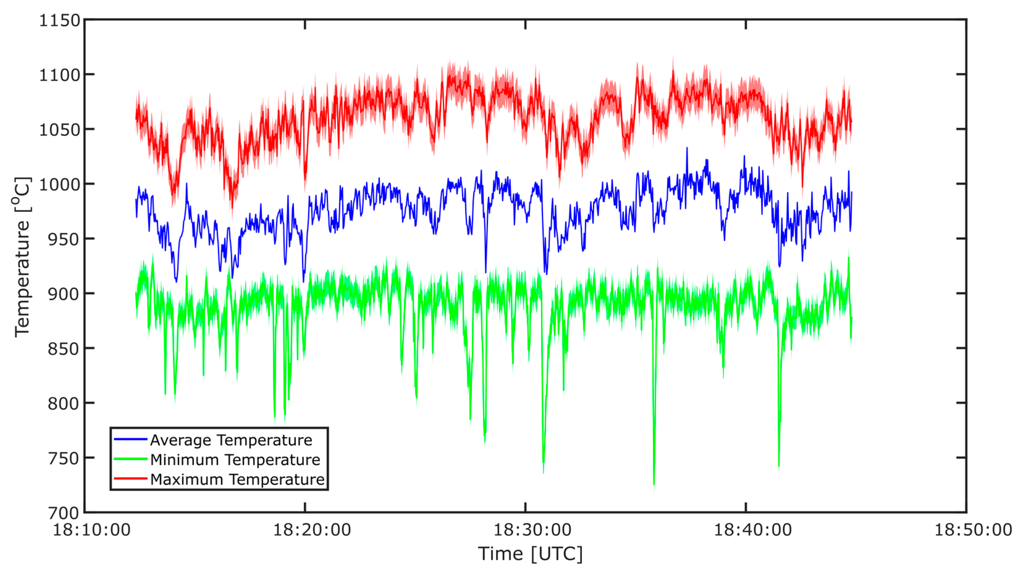
The camera system was deployed at Masaya Volcano, Nicaragua, where a lava lake has been visible in the Santiago crater since 2015. Masaya is a basaltic volcano which stands at an altitude of 635 m in the west of Nicaragua, approximately 20 km south-east of the capital Managua. The volcano is currently displaying a vigorously overturning lava lake, one of fewer than 10 known current lava lakes on Earth. Nevertheless, to the best of our knowledge there are currently no articles in the scientific literature which report ground-based data on the thermal characteristics of this most recent phase of Masaya’s activity.
Between 12 and 17 June 2017, a range of tests were performed with the thermal imaging PiCam. Here, we discuss a dataset from 12 June, acquired after sundown; therefore, any uncertainty due to reflected solar radiation was avoided. Images were acquired at a framerate 0.5 Hz. Due to extracting the RAW sensor data here, which is packed into the start of the standard JPEG files, this framerate is at the upper limit of what is currently achievable with our software. One significant advantage of previous PiCam work by Radebaugh et al. [12] is the high framerate afforded by use of the video port. Current work to directly access the RAW sensor data, bypassing image post-processing on the board itself, could open up much higher framerates for our system in the future.
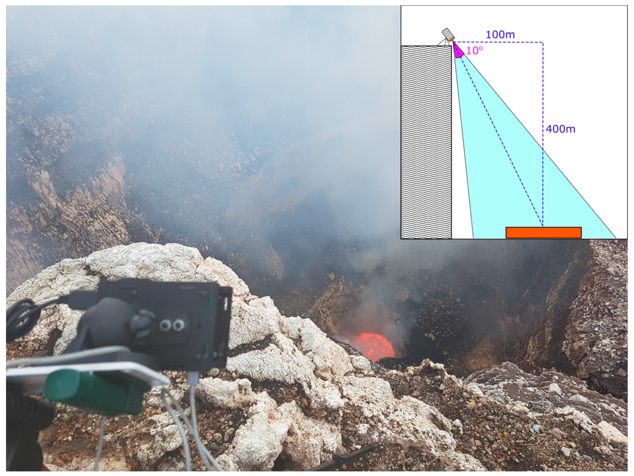
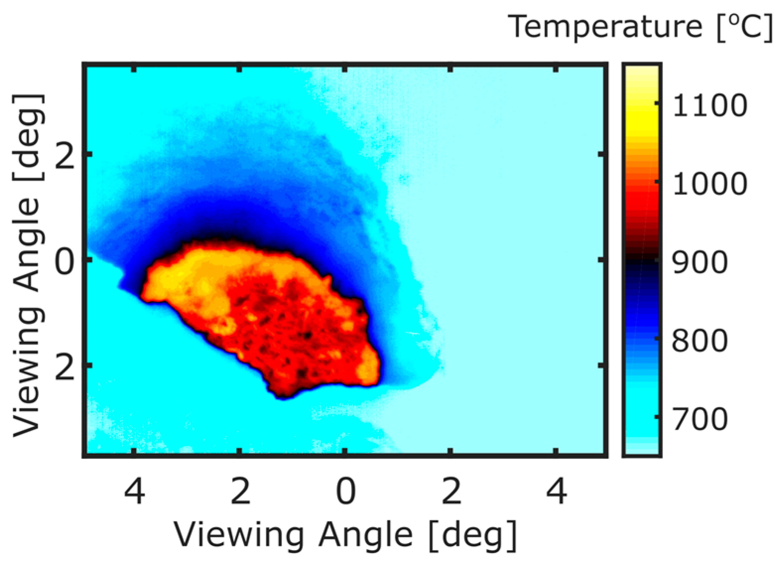
The viewing platform was located approximately 400 m above the lake; viewing geometry is displayed in Figure 2. From this position, a region of the lava lake is obscured by a crater terrace and, thus, it should be noted that work presented here does not represent measurements of the entire exposed lava lake surface.
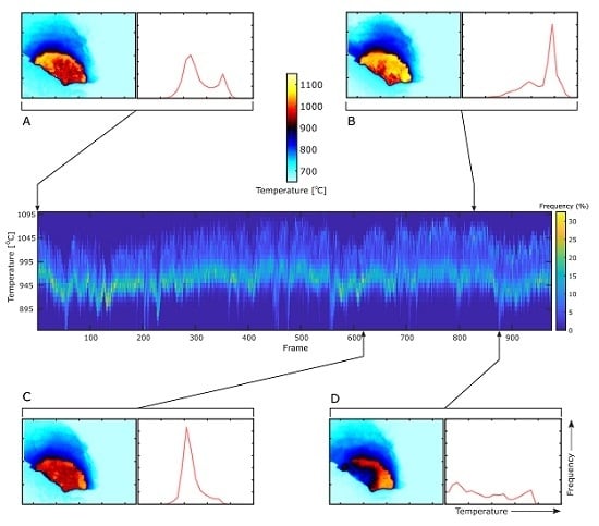
To accurately interrogate the lava lake and its thermal features it is important to isolate the lake from its surroundings; however, due to windy conditions, there is a relatively significant camera shake apparent in the image sequences (Video S1). Two methods were therefore tested for defining the lava lake region of interest (ROI) in each frame. Firstly, the image sequences were stabilised by utilising a Lucas-Kanade image registration [33] of each frame to the template of the first frame; this was implemented in Matlab using the Image Alignment Toolbox [34]. From here, a ROI, i.e., the lava lake, can be extracted by defining its extent with a polygon; for each subsequent frame the same polygon is then extracted. However, the image registration in most cases here was not perfect, possibly due to the fast-flowing lava lake and intermittent presence of aerosols, as well as the difficulty in finding optimal input parameters for this algorithm. Some camera shake is, therefore, still observable in a video stabilised in this manner (Video S2); although the larger image shifts have been removed, it appears that smaller shake has been exacerbated. We therefore attempted to define the lava lake in a separate manner, using a threshold of any temperature above 850 °C representing the lake. This temperature was determined first by a best estimate and refined by observing how the resultant threshold mask visibly compares to the lake surface. A video of this threshold mask shows that in places it can provide an accurate determination of the lava lake extent, where clearly defined edge features are tracked from frame to frame (Video S3); however, in regions where there is spattering at the lake edges, or intense scattering from aerosols, the lava lake can become over or under-defined; the former issue is also commented on in Radebaugh et al. [12]. For the data discussed in this article we apply the first method, image registration, since we believe this to be the most robust method in most cases; it also has the potential to be much improved relative to our example here. However, there are a number of studies in which thresholding could be extremely useful, for example, for calculating the extent of cooled plates within a lava lake, or where there is minimal aerosol and spattering such that the lava lake boundary can easily be defined by a temperature contrast with the surrounding crater wall.

3. Results and Discussion

An example thermal image of Masaya Lava Lake is shown in Figure 5. In general, the quality of image is high, with cooled plates and bubble bursts well defined/resolved. On parts of the crater walls, extremely high temperatures (750–850 °C) are retrieved. However, rather than being caused by high temperature emission, this signal comes from the scattering/reflection of radiation by the walls themselves or aerosols from the volcanic plume. The retrieved temperatures in this case are, therefore, erroneous.
General interrogation of the thermal imagery and associated ROI time series, taken on 12 June from 18:12:20 to 18:44:48 UTC, indicates a mean lava lake temperature, averaged over both space and time, of ≈970 °C (Figure 6). The uncertainty associated with a single pixel at this temperature is ±12 °C; however, since here a mean temperature is quoted, this uncertainty is not directly applicable. Freshly exposed magma, from bubble bursting events or collision of the lake with the crater wall, reaches temperatures of up to ≈1104 ± 14 °C, which is relatively consistent with temperatures recorded for molten basalts at other lava lakes (e.g., [3,12,35,36]).
Periods of time which are heavily affected by aerosol display a significant decrease in minimum temperature within the ROI (Figure 6). It may, therefore, be possible to set a minimum temperature threshold, whereby any frame where a pixel within the ROI drops below this threshold is flagged and can be discarded from further analysis. Here, however, since we do not perform any detailed lake dynamics analyses, we do not perform this procedure. Unless the aerosols are causing dramatic changes to the temperature time series, as discussed above, it is difficult to determine when aerosols are having an effect on retrievals. Interrogating the thermal imagery as well as temperature histograms (presented later) may also provide insights into periods where aerosols are interfering with retrievals. In general, however, we must assume that for times other than those mentioned above aerosol effects are not significant. Although this issue is possibly less significant at MWIR/LWIR wavelengths, such assumptions must still be made when using these longer wavelength instruments and are unavoidable without more detailed knowledge of the conditions along the instrument’s viewing path.
The lava lake area is estimated from the viewing geometry and, thus, radiative power output, Q (W), is calculated using the Stefan-Boltzmann law:
Q =   ε σ i = 0 n A i T i 4
where A i and T i are the area (m2) and temperature (K) of the ith pixel, σ is the Stefan-Boltzmann constant and ε is the emissivity. We calculate Masaya lava lake to have an average radiative power output of 37 MW (Figure 7), a value which is on the order of 1–10% of common power station outputs. Aiuppa et al. [20] used the Moderate Resolution Imaging Spectroradiometer (MODIS), evaluated by Middle Infrared Observation of Volcanic Activity (MIROVA), to quantify Masaya’s radiative power output between May 2016 and March 2017, quoting an average of 60.8 MW. Our measurements, made just 3 months later, are comparable to this, somewhat corroborating our findings. These results are comparable to a number of other lava lake radiative fluxes, which have been quantified previously using both ground-based and satellite imagery (Table 2), although a large range is present. In particular, Masaya has quite similar radiative power output to past measurements of both Erebus and Erta ‘Ale; this results from Masaya’s significantly higher average lake surface temperature but much smaller surface area (≈280 m2 visible in images presented herein). The fluxes are considerably smaller than those of Nyiragongo, which has an extremely large radiating surface area (31,400 m2; [35]). There are, however, large uncertainties in our measurement, relating to the dimensions of the lava lake which were calculated from the roughly estimate viewing geometry. Accurate path length measurements, using LiDAR for example, would be needed to give a more robust estimation of the lake’s radiative power output. Furthermore, it should be noted that the lake was quite turbulent and, therefore, at times it is not accurately represented by a flat surface assumption. In addition, the entire lake surface is not visible in the images presented herein, since a proportion is obscured by crater walls. The radiating surface area is, therefore, likely to be significantly larger than estimated here; thus, estimations of radiative power likely serve as only lower limits to the true values.
Similar to the RadTherm plots of Coppola et al. [44], we display a temperature histogram time series, with a colour scale Z-axis displaying the frequency of pixels in each temperature bin (Figure 8); essentially, temperature histograms (Figure 9) have been assimilated such that their variation through time can be assessed. This can be an extremely useful way of displaying and interrogating thermal datasets, since it is relatively easy to identify significant changes in the volcanic system, or specific images which may be of particular interest.
During periods of high activity, from either a cluster of bubble burst events or increased turbulence at the wall edges, both of which expose fresh molten lava, a significant increase in the modal temperature is displayed in Figure 8B and the higher temperature bins become more populated. Slightly more stable periods in the lake are characterized by a bimodal temperature distribution where parts of the lake have cooled to form plates whilst other regions have freshly exposed molten lava from turbulence and bubble bursts; the top left panel (Figure 8A) presents an exemplary image of this state. Images which are affected by significant extinction from aerosols can also often be identified through significantly lower temperatures. Such dips are present in a few places in the time series presented here and Figure 8D shows an example of this behaviour. Figure 9 shows that the general lava lake state is a weak positive skew, an example of which is shown in Figure 8C. This suggests that the majority of the time the lava lake is in a relatively stable state, with a gradually cooling crust disrupted by a few bubble bursts; these bursts provide the higher temperatures which positively skew an otherwise Gaussian cooling surface.

4. Concluding Remarks

We have presented and discussed the development of a new low-cost, NIR thermal camera based on a modified Raspberry Pi camera module. This work builds upon previous articles which have utilised consumer electronics silicon sensors, primarily designed for visible imagery, as high temperature thermal cameras. The modified sensor has heightened NIR sensitivity, is free from the mosaic response caused by the presence of a Bayer Filter in standard visible imaging cameras and provides 10-bit images. Furthermore, our rigorous calibration, using a blackbody furnace and a Sakuma-Hattori model fit, should provide accurate temperature retrievals. We suggest that the presented system will work well for high temperature applications (≥500 °C) and, thus, could provide a good low-cost alternative to commercial thermal imaging cameras for many aspects of volcanology as well as a range of other fields. It is important to note that for temperatures close to 500 °C solar reflections may become significant; therefore, imaging at night or applying a solar correction could be necessary for accurate retrievals.
We have discussed and quantified a number of uncertainties, caused by both the calibration procedure and the sensor itself, as well as considering emissivity and path transmission issues. In our case, the flat-field uncertainty is most significant at higher temperatures; we therefore suggest that a flat-field correction would be desirable. Due to the spectral range of the camera (≈850–1100 nm), uncertainties associated with atmospheric absorption are shown to be relatively small under the conditions experienced on Masaya during this campaign; however, we still suggest that a single correction for this factor is applied. In general, it is likely that path lengths and atmospheric/plume conditions are much less of a concern than when trying to retrieve accurate temperatures with mid-/long-wavelength infrared systems, where CO2 and H2O have relatively large absorption features. Difficulties were, however, encountered when the volcanic plume was highly condensed; therefore, this must be considered when determining appropriate sites for deployment of this instrument.
We tested the system on Masaya volcano, Nicaragua, where an active lava lake has been present since 2015. The mean surface temperature of the lake was determined to be ≈970 °C, with a maximum temperature of 1104 ± 14 °C being retrieved. The radiative power output of the lake ranged from 30 to 45 MW, with an estimated area of 280 m2. To the best of our knowledge, this report is the first published ground-based thermal data on Masaya’s lava lake, since it emerged in late 2015.

Supplementary Materials

The following are available online at https://www.mdpi.com/2072-4292/10/3/450/s1, Video S1: A video of temperatures from the lava lake, acquired on 12 June 2017, between 17:44 and 18:11 UTC. Significant camera shake is evident; Video S2: A stabilised version of Video S1. The video has been stabilised with the Lukas-Kanade method discussed in Section 2.5. Although small scale shake can still be seen, this represents a notable improvement on the larger frame shifts present in the raw video frame; Video S3: A threshold video produced from the data in Video S1. A temperature threshold of 850 °C is used, such that all pixels above this value are displayed in red and all below are displayed as blue. It is evident that in places this thresholding tracks the shake of the camera, defining the edge of the lava lake well; this is particularly good on the right-hand side. However, in regions where aerosols are abundant, or there is significant spattering and heating of the crater wall, this threshold does not accurately define the lake outline.

Acknowledgments

We greatly acknowledge the sponsors of this work. We thank INETER for their help with access to Masaya volcano and in particular Wilfried Strauch for logistical assistance. T.C.W. acknowledges a Department of Geography, University of Sheffield, studentship. J.R.W. acknowledges the support of an Engineering and Physical Sciences Research Council grant (EP/M009106/1). AMcG acknowledges a Leverhulme Research Fellowship (RF-2016-580) and the Rolex Institute. T.D.P. acknowledges the support of the Royal Society (RG170226).

Author Contributions

A.J.S.M., J.R.W. and T.C.W. conceived the idea. J.R.W. and T.C.W. designed and built the instrument. L.R.S. performed the calibration and uncertainty analysis. T.D.P. led the field campaign; T.C.W. and R.A.E. aided in fieldwork. Data analyses were predominantly performed by T.C.W. T.C.W. wrote the paper, with valuable contributions from all authors.

Conflicts of Interest

The authors declare no conflict of interest.

Appendix A

In this section, we quantify the effects of solar radiation on measurements made using our NIR system. We model the reflected solar radiance from the lake, thereby calculating the proportion of sensor signal originating from reflections rather than the lake’s emitted radiation. We use the reference air mass 1.5 solar spectral irradiance data provided by the American Society for Testing and Materials (ASTM) retrieved from http://rredc.nrel.gov/solar/spectra/am1.5/. This models the spectra using the Simple Model for Atmospheric Transmission of Sunshine (SMARTS2 v 2.9.2) developed by Gueymard [45]. The model provides the spectral irradiance at the earth’s surface assuming a cloudless sky; hence, solar influences presented here will be worst-case scenarios of atmospheric conditions. The irradiance is calculated for a plane inclined towards the sun at 37° towards the equator, at a solar zenith angle of 48.19°; this will cause an over estimation of the solar irradiance on a surface parallel to the ground.
Assuming direct sunlight is incident on the lava lake, under the assumption of Lambertian reflectance, the reflected spectral radiance is calculated by:
L R ( λ ) =   α I S ( λ ) π
where α is the surface reflectance ( 1   ε ), I S ( λ ) is the solar spectral irradiance incident on the lake and L R ( λ ) is the reflected spectral radiance. The emitted spectral irradiance L E ( λ ) , at a given temperature is then calculated using Planck’s law for black body emission and scaled by the emissivity ε .
Both the reflected and emitted spectral radiances are then filtered by the normalized responsivity of our PiCam instrument (as in Section 2.3). The total radiances of each contribution, calculated by integrating the spectral radiances over the instrument’s response band (0.85–1.15 μm), can then be used to determine the relative contribution of reflected solar radiation P R , to the signal measured by the PiCam:
P R =   L R L R +   L E
where L R and L E are the reflected and emitted radiances, respectively.
For a range of pertinent temperatures, we use Equation (1) to find the associated measured signal, then use P to determine the signal associated with both emitted and reflected radiation from the lake. We are thus able to calculate the temperature of the lake itself or, similarly, determine the temperature error caused by reflected solar radiation (Figure A1). All calculations assumed a path transmission coefficient of β = 0.8789 , as in Section 2.3.
Figure A1. (A) Temperature errors associated with solar reflection vs. emissivity, for a range of temperatures. (B) As in (A) but for a much lower temperature of 500 °C. For lava lake temperatures presented in this article (predominantly 900–1100 °C) errors caused by solar reflections are minimal (all < 6 °C) for emissivities > 0.9. At much lower temperatures (500 °C) the solar effect is much more significant, even at emissivities approaching 1; therefore, it is likely that applications imaging such temperatures would need to be either away from direct sunlight, at night, or possibly with a sophisticated correction for solar radiance.
Remotesensing 10 00450 g0a1
It can be seen that the error caused by solar reflections is relatively small (<6 °C) for lava lake temperatures presented herein, assuming an emissivity of greater than 0.9. Moreover, in scenarios where the emissivity is considerably lower the temperature, error remains less than 10 °C at high temperatures (≈>1100 °C). It is also important to reiterate that this model assumes a cloudless sky and that the imaged object (i.e., the lake in this case) is directly illuminated by the sun on an inclined plane. The majority of the time, therefore, solar contributions will be considerably less than those presented here.
For lower temperature applications (≈500 °C), Figure A1B highlights that the solar contribution is significantly greater, causing errors of >100 °C for emissivities less than 0.95; the error remains high for emissivities greater than 0.95 until it reduces to 0 at ε = 1 , as required by Kirchoff’s Law. This result suggests that lower temperature applications would benefit significantly from being performed at night, or they may still be feasible in daytime if direct sunlight is avoided. This model does not consider the effects of diffuse sky radiation on temperature retrievals and, thus, it is difficult to provide detailed comments on imaging under such conditions. Alternatively, it may be possible to develop a sunlight correction scheme, which would enable imaging of relatively low temperature targets even in direct sunlight. A more sophisticated time of year and time of day dependent model can be made, which would give a representative contribution to the measured radiance of a reflecting pool. Or more precisely, the spectral irradiance close to a target could be directly measured by another instrument, making a correction relatively straightforward.

Appendix B

In Table A1 we present the calibration and uncertainty fit parameters for the PiCam discussed in this paper, using a shutter speed of 1 ms; these values apply to the system with the 850 nm long-pass filter mounted in place and no band-pass filters included. It should be noted that these values were empirically determined and are specific to the instrument and calibration performed herein. Therefore, any subsequent work will need to calculate these parameters independently and it should be expected that they may differ considerably.
Table A1. Table of calibration and uncertainty fit parameters for 1 ms shutter speed.
ParameterValueUsed in Equation
A01.35 × 10−81–3
A18.6697 × 10−71–3
A23.90586 × 10−51–3
σ f i t [°C]1.084
B00.69665
B10.0025945
C00.10986
C10.15456
The standard error, σ f i t , is given by the standard deviation of the Sakuma-Hattori fit residuals.

Appendix C

Although already examined in Wilkes et al. [15], here we again had an opportunity to evaluate the linearity of the sensor’s response with respect to incident radiation. Furthermore, the test here is more robust than the clear-sky imaging in the former paper, since the radiance from the black-body furnace is likely to be much more stable than that from the clear-sky, the latter of which is highly dependent on atmospheric conditions. It would be expected that the sensor responds linearly and this characteristic is a necessity for accurate radiometric applications. Since a wide range of shutter speeds were used in the field with the 1080 nm band-pass filter mounted to the fore of the optical system (as mentioned in Section 2.3), our linearity tests utilise the calibrations from this optical setup, rather than the single 850 nm long-pass filter setup, which is the arrangement used to gather the majority of the data discussed in this article. Although the filter arrangements are slightly different, this should not affect the linearity tests presented here; therefore, it is reasonable to assume that the results also relate to the 850 nm long-pass filter setup.
Figure A2 displays the results of imaging a blackbody furnace at a range of shutter speeds and for a number of temperatures. Each data point represents an average Digital Number (DN) from 30 images taken at that shutter speed and temperature. The values are therefore averaged in both the spatial and temporal domains. The lines represent a best fit from a linear regression, which all have extremely high r2 values (r2 > 0.99) but do not all intersect close to the origin; in particular, at 950 °C, for an unknown reason the dark current subtraction has shifted the regression to intersect well below the origin, at a DN of ≈ −8.6. By forcing the regression through the origin, we degrade the quality of the fit. We believe it is this error which affects the quality of the second calibration method discussed in Section 2.2.
Figure A2. A plot of Digital Number (DN) vs. Shutter Speed (ms), where the DN is found from an average of 30 images taken imaging the blackbody furnace at the specified temperature. Error bars represent the associated uncertainty of this 30-member mean. The optical system used for this test had the 1080 nm band-pass filter mounted to the fore of the system, as well as the 850 nm long pass filter mounted behind the lens triplet.
Remotesensing 10 00450 g0a2

References

  1. Spampinato, L.; Calvari, S.; Oppenheimer, C.; Boschi, E. Volcano surveillance using infrared cameras. Earth Sci. Rev. 2011, 106, 63–91. [Google Scholar] [CrossRef]
  2. Patrick, M.R.; Orr, T.; Antolik, L.; Lee, L.; Kamibayashi, K. Continuous monitoring of Hawaiian volcanoes with thermal cameras. J. Appl. Volcanol. 2014, 3, 1. [Google Scholar] [CrossRef]
  3. Oppenheimer, C.; Yirgu, G. Thermal imaging of an active lava lake: Erta ‘Ale volcano, Ethiopia. Int. J. Remote Sens. 2002, 23, 4777–4782. [Google Scholar] [CrossRef]
  4. Peters, N.; Oppenheimer, C.; Killingsworth, D.R.; Frechette, J.; Kyle, P. Correlation of cycles in Lava Lake motion and degassing at Erebus Volcano, Antarctica. Geochem. Geophys. Geosyst. 2014, 15, 3244–3257. [Google Scholar] [CrossRef]
  5. Delle Donne, D.; Ripepe, M. High-frame rate thermal imagery of strombolian explosions: Implications for explosive and infrasonic source dynamics. J. Geophys. Res. Solid Earth 2012, 117, B09206. [Google Scholar] [CrossRef]
  6. McGonigle, A.J.S.; Aiuppa, A.; Giudice, G.; Tamburello, G.; Hodson, A.J.; Gurrieri, S. Unmanned aerial vehicle measurements of volcanic carbon dioxide fluxes. Geophys. Res. Lett. 2008, 35, 3–6. [Google Scholar] [CrossRef]
  7. Amici, S.; Turci, M.; Giulietti, F.; Giammanco, S.; Buongiorno, M.F.; La Spina, A.; Spampinato, L. Volcanic environments monitoring by drones, Mud Volcano case Study. Int. Arch. Photogramm. Remote Sens. Spat. Inf. Sci. 2013, XL-1/W2, 5–10. [Google Scholar] [CrossRef]
  8. Mori, T.; Hashimoto, T.; Terada, A.; Yoshimoto, M.; Kazahaya, R.; Shinohara, H.; Tanaka, R. Volcanic plume measurements using a UAV for the 2014 Mt. Ontake eruption. Earth Planets Space 2016, 68, 49. [Google Scholar] [CrossRef]
  9. Chio, S.H.; Lin, C.H. Preliminary study of UAS equipped with thermal camera for volcanic geothermal monitoring in Taiwan. Sensors 2017, 17, 1649. [Google Scholar] [CrossRef] [PubMed]
  10. Saito, T.; Sakai, S.; Iizawa, I.; Suda, E.; Umetani, K.; Kaneko, K.; Furukawa, Y.; Ohkura, T. A new technique of radiation thermometry using a consumer digital camcorder: Observations of red glow at Aso volcano, Japan. Earth Planets Space 2005, 57, 5–8. [Google Scholar] [CrossRef]
  11. Furukawa, Y. Infrared thermography of the fumarole area in the active crater of the Aso volcano, Japan, using a consumer digital camera. J. Asian Earth Sci. 2010, 38, 283–288. [Google Scholar] [CrossRef] [Green Version]
  12. Radebaugh, J.; Lopes, R.M.; Howell, R.R.; Lorenz, R.D.; Turtle, E.P. Eruptive behavior of the Marum/Mbwelesu lava lake, Vanuatu and comparisons with lava lakes on Earth and Io. J. Volcanol. Geotherm. Res. 2016, 322, 105–118. [Google Scholar] [CrossRef]
  13. Dixon, J. Radiation Thermometry; John Wiley & Sons: Hoboken, NJ, USA, 1988. [Google Scholar]
  14. Ball, M.; Pinkerton, H. Factors affecting the accuracy of thermal imaging cameras in volcanology. J. Geophys. Res. Solid Earth 2006, 111, B11203. [Google Scholar] [CrossRef]
  15. Wilkes, T.C.; McGonigle, A.J.S.; Pering, T.D.; Taggart, A.; White, B.; Bryant, R.; Willmott, J.R. Ultraviolet Imaging with Low Cost Smartphone Sensors: Development and Application of a Raspberry Pi-Based UV Camera. Sensors 2016, 16, 1649. [Google Scholar] [CrossRef] [PubMed]
  16. Gunturk, B.K.; Glotzbach, J.; Altunbasak, Y.; Schafer, R.W.; Mersereau, R.M. Demosaicking: Color filter array interpolation. IEEE Signal Process. Mag. 2005, 22, 44–54. [Google Scholar] [CrossRef]
  17. Patrick, M.R.; Orr, T.; Lee, L.; Moniz, C.J. A Multipurpose Camera System for Monitoring Kilauea Volcano, Hawai’i; U.S. Geological Survey: Reston, VA, USA, 2015.
  18. Wilkes, T.C.; Pering, T.D.; McGonigle, A.J.S.; Tamburello, G.; Willmott, J.R. A Low-Cost Smartphone Sensor-Based UV Camera for Volcanic SO2 Emission Measurements. Remote Sens. 2017, 9, 27. [Google Scholar] [CrossRef]
  19. Wilkes, T.C.; McGonigle, A.J.S.; Willmott, J.R.; Pering, T.D.; Cook, J.M. Low-cost 3D printed 1  nm resolution smartphone sensor-based spectrometer: Instrument design and application in ultraviolet spectroscopy. Opt. Lett. 2017, 42, 4323. [Google Scholar] [CrossRef] [PubMed]
  20. Aiuppa, A.; de Moor, J.M.; Arellano, S.; Coppola, D.; Francofonte, V.; Galle, B.; Giudice, G.; Liuzzo, M.; Mendoza, E.; Saballos, A.; et al. Tracking Formation of a Lava Lake From Ground and Space: Masaya Volcano (Nicaragua), 2014–2017. Geochem. Geophys. Geosyst. 2018, 2014–2017. [Google Scholar] [CrossRef]
  21. Report on Masaya (Nicaragua). In Bulletin of the Global Volcanism Network; Venzke, E. (Ed.) Smithsonian Institution: Washington, DC, USA, 2017; Volume 42. [Google Scholar]
  22. Lane, B.; Whitenton, E.P. Calibration and Measurement Procedures for a High Magnification Thermal Camera; National Institute of Standards and Technology: Gaithersburg, MD, USA, 2015. [CrossRef]
  23. Saunders, P.; White, D.R. Physical basis of interpolation equations for radiation thermometry. Metrologia 2003, 40, 195–203. [Google Scholar] [CrossRef]
  24. Sawyer, G.M.; Burton, M.R. Effects of a volcanic plume on thermal imaging data. Geophys. Res. Lett. 2006, 33, L14311. [Google Scholar] [CrossRef]
  25. Gordon, I.E.; Rothman, L.S.; Hill, C.; Kochanov, R.V.; Tan, Y.; Bernath, P.F.; Birk, M.; Boudon, V.; Campargue, A.; Chance, K.V.; et al. The HITRAN2016 molecular spectroscopic database. J. Quant. Spectrosc. Radiat. Transf. 2017, 203, 3–69. [Google Scholar] [CrossRef]
  26. Pliutau, D.; Roslyakov, K. Bytran -|- spectral calculations for portable devices using the HITRAN database. Earth Sci. Inform. 2017, 10, 395–404. [Google Scholar] [CrossRef]
  27. Kochanov, R.V.; Gordon, I.E.; Rothman, L.S.; Wcisło, P.; Hill, C.; Wilzewski, J.S. HITRAN Application Programming Interface (HAPI): A comprehensive approach to working with spectroscopic data. J. Quant. Spectrosc. Radiat. Transf. 2016, 177, 15–30. [Google Scholar] [CrossRef]
  28. Pinkerton, H.; James, M.; Jones, A. Surface temperature measurements of active lava flows on Kilauea volcano, Hawai’i. J. Volcanol. Geotherm. Res. 2002, 113, 159–176. [Google Scholar] [CrossRef]
  29. Rothery, D.A.; Francis, P.W.; Wood, C.A. Volcano Monitoring Using Short Wavelength Infrared Data from Satellites. J. Geophys. Res. 1988, 93, 7993–8008. [Google Scholar] [CrossRef]
  30. Ripepe, M.; Harris, A.J.L.; Marchetti, E. Coupled thermal oscillations in explosive activity at different craters of Stromboli volcano. Geophys. Res. Lett. 2005, 32, L17302. [Google Scholar] [CrossRef]
  31. Lane, B.; Whitenton, E.; Madhavan, V.; Donmez, A. Uncertainty of temperature measurements by infrared thermography for metal cutting applications. Metrologia 2013, 50, 637–653. [Google Scholar] [CrossRef]
  32. Du, H.; Voss, K.J. Effects of Point-Spread Function on Calibration and Radiometric Accuracy of CCD Camera. Appl. Opt. 2004, 43, 665. [Google Scholar] [CrossRef] [PubMed]
  33. Baker, S.; Matthews, I. Lucas-Kanade 20 years on: A unifying framework. Int. J. Comput. Vis. 2004, 56, 221–255. [Google Scholar] [CrossRef]
  34. Evangelidis, G. IAT: A Matlab Toolbox for Image Alignment. Available online: https://sites.google.com/site/imagealignment/ (accessed on 10 November 2017).
  35. Spampinato, L.; Ganci, G.; Hernández, P.A.; Calvo, D.; Tedesco, D.; Pérez, N.M.; Calvari, S.; Del Negro, C.; Yalire, M.M. Thermal insights into the dynamics of Nyiragongo lava lake from ground and satellite measurements. J. Geophys. Res. Solid Earth 2013, 118, 5771–5784. [Google Scholar] [CrossRef]
  36. Carling, G.T.; Radebaugh, J.; Saito, T.; Lorenz, R.D.; Dangerfield, A.; Tingey, D.G.; Keith, J.D.; South, J.V.; Lopes, R.M.; Diniega, S. Temperatures, thermal structure, and behavior of eruptions at Kilauea and Erta Ale volcanoes using a consumer digital camcorder. GeoResJ 2015, 5, 47–56. [Google Scholar] [CrossRef]
  37. Harris, A.J.L.; Flynn, L.P.; Rothery, D.A.; Oppenheimer, C.; Sherman, S.B. Mass flux measurements at active lava lakes: Implications for magma recycling. J. Geophys. Res. 1999, 104, 7117–7136. [Google Scholar] [CrossRef]
  38. Calkins, J.; Oppenheimer, C.; Kyle, P.R. Ground-based thermal imaging of lava lakes at Erebus volcano, Antarctica. J. Volcanol. Geotherm. Res. 2008, 177, 695–704. [Google Scholar] [CrossRef]
  39. Le Guern, F.; Carbonnelle, J.; Tazieff, H. Erta’Ale lava lake: Heat and gas transfer to the atmosphere. J. Volcanol. Geotherm. Res. 1979, 6, 27–48. [Google Scholar] [CrossRef]
  40. Oppenheimer, C.; McGonigle, A.J.S.; Allard, P.; Wooster, M.J.; Tsanev, V. Sulfur, heat, and magma budget of Erta ’Ale lava lake, Ethiopia. Geology 2004, 32, 509–512. [Google Scholar] [CrossRef]
  41. Spampinato, L.; Oppenheimer, C.; Calvari, S.; Cannata, A.; Montalto, P. Lava lake surface characterization by thermal imaging: Erta ’Ale volcano (Ethiopia). Geochem. Geophys. Geosyst. 2008, 9, Q12008. [Google Scholar] [CrossRef]
  42. Cipar, J.J.; Anderson, G.P.; Cooley, T.W. Temperature and power output of the lava lake in Halema’uma’u crater, Hawaii, using a space-based hyperspectral imager. IEEE J. Sel. Top. Appl. Earth Obs. Remote Sens. 2012, 5, 617–624. [Google Scholar] [CrossRef]
  43. Le Guern, F. Mechanism of Energy Transfer in the Lava Lake of Niragongo (Zaire), 1959–1977. J. Volcanol. Geotherm. Res. 1987, 31, 17–31. [Google Scholar] [CrossRef]
  44. Coppola, D.; Staudacher, T.; Cigolini, C. Field thermal monitoring during the August 2003 eruption at Piton de la Fournaise (La Réunion). J. Geophys. Res. Solid Earth 2007, 112, B05215. [Google Scholar] [CrossRef]
  45. Gueymard, C.A. Parameterized transmittance model for direct beam and circumsolar spectral irradiance. Sol. Energy 2001, 71, 325–346. [Google Scholar] [CrossRef]
Figure 1. (A) Lens design in OpticStudio (Zemax Ltd.) showing the position of each lens in the triplet, the aperture, filter and sensor from the PiCam. Colours represent light rays terminating at different field heights on the focal plane array; red displays the rays at the edge of the camera field of view (5° from the optical axis), whilst blue represents rays parallel to the optical axis. (B) Image of the 3D printed lens holder and camera mount. The filter holder slides into the camera mount during operation. The triplet lens holder is threaded and thus can be focused (at infinity) in the field.
Remotesensing 10 00450 g001
Figure 2. Main image: Photograph of the PiCam capturing images of the lava lake at Masaya volcano on 12 June 2017. The plume aerosols are quite clearly visible, as are bubble bursts in the lake itself. Inset: A schematic of the estimated viewing geometry provided by Instituto Nicaragüense de Estudios Territoriales (INETER; Personal Communication, 2017); figure not to scale.
Remotesensing 10 00450 g002
Figure 3. (A) A plot showing how retrieved temperature varies with emissivity of the object. Displayed at 3 different Digital Numbers (DNs), for a shutter speed of 1 ms and with a path transmission coefficient of 0.8789. (B) As (A) but displaying the effect of a water vapour correction on the retrieved temperature, i.e., larger estimated water vapour loadings in the path cause higher temperatures to be retrieved since there is more absorption of radiation across the path. For each data point the transmission coefficient was calculated as the mean between 800–1200 °C (see Section 2.3 for further explanation). Data is plotted for an emissivity of 0.95, with atmospheric temperature and pressure of 26.5 °C and 94,300 Pa, respectively; relative humidity is quoted using a path length of 412 m, used in the field tests on Masaya volcano (see Section 2.5).
Remotesensing 10 00450 g003
Figure 4. Calculated measurement uncertainties vs measured temperature for 1 ms exposure time on the PiCam. As in the discussion of Section 2.4, all uncertainties are for a 95% confidence interval. For the majority of uncertainties, a larger temperature is concomitant with larger measurement uncertainty, apart from the sensor noise uncertainty, since the signal-to-noise ratio increases with increasing signal/temperature; longer exposure times will decrease the sensor noise uncertainty for a given temperature and, thus, somewhat extend the use of this system to lower temperatures. Since flat-field uncertainty could be corrected for and emissivity could possibly be more accurately constrained than in this study, the minimum uncertainties of this technique are likely constrained by the sensor noise and calibration uncertainties.
Remotesensing 10 00450 g004
Figure 5. A PiCam image of the Masaya lava lake, taken on 12 June 2017 at 18:12:20 UTC. Lake temperatures of up to 1059 ± 14 °C are observed here. Temperatures are highest towards the edges where collisions with the crater wall appear to occur and elsewhere in the lake when bubble bursts expose fresh magma. The high apparent temperature of the crater wall is due to reflection of the lake’s radiation, either by aerosols or by the wall itself; these temperatures are, therefore, inaccurate.
Remotesensing 10 00450 g005
Figure 6. Temperature time series from 18:12:20 to 18:44:48 UTC on 12 June 2017, taken with a 1 ms shutter speed at a framerate of 0.5 Hz. Maximum, minimum and average temperatures of the lava lake region of interest (ROI) and displayed. Maximum and minimum temperatures have associated total uncertainties displayed as a shaded region.
Remotesensing 10 00450 g006
Figure 7. Radiant flux time series from 18:12:20 to 18:44:48 UTC on 12 June 2017. The flux ranges from 30 to 45 MW, with an average of 37 MW. The lake area, used in this calculation (Equation (11)), was estimated to be 280 m2.
Remotesensing 10 00450 g007
Figure 8. A stack of lava lake temperature histograms (central pane), similar to the RadTherm plots of Coppola et al. [44]. Surrounding subplots display lava lake thermal images and the associated temperature histograms; for ease of comparison, all histograms are plotted on the same axis scale, as in Figure 9. Subplots show examples of: (A) bimodal temperature distribution due to a relatively large amount of spattering at the lake edge and the cooler crust surface; (B) extremely hot temperatures due to high levels of edge spattering and large bubble bursts exposing fresh hot lava; (C) weak-positively skewed distribution of temperatures due to a relatively undisturbed cooled crust, along with small bubble bursts; (D) aerosol extinction obscuring the view of the lava lake and, thus, causing significantly lower retrieved temperatures. Note that the frequency colour scale relates to the central stacked histogram figure, whilst the temperature colour scale relates to the lava images.
Remotesensing 10 00450 g008
Figure 9. Histograms of temperature distributions, in 10 °C bins, across the lava lake from 18:12:20 to 18:44:48 UTC on 12 June 2017. The lava lake area was defined by a user-defined region of interest. For clarity, histograms are coloured by the frame time they represent; earlier frames are more blue and later frames are more red. The bold yellow line represents the mean distribution, which is a slight positive skew. This is likely due to bubble bursts and lake turbulence which introduce hotter lava into what otherwise would be a steadily cooling crust which you may expect to display a Gaussian temperature distribution.
Remotesensing 10 00450 g009
Table 1. Calibration Uncertainties.
UncertaintySymbolQuantification
Thermocouple uncertainty σ T c B B 0.4 °C
Blackbody cavity temperature uncertainty σ T B B 1 °C
Blackbody emissivity uncertainty σ ε B B 0.04   × S m e a s × S m e a s T 1 *
Fit uncertainty σ f i t Standard error of Sakuma-Hattori fit (see Table A1 for value at 1 ms shutter speed)
* See Equation (3) for calculation of S m e a s T 1 .
Table 2. Assimilation of lava lake radiant power data, associated lake areas and the instrument used for the retrieval. Only relatively high-resolution instruments are included here, such that studies which calculate radiant power from sub-pixel scale lava lakes are omitted.
Volcano YearInstrumentArea (m2)Radiant Power (MW)Reference
Masaya
2017GB NIR camera28030–45This article
Erebus
1985Landsat TM18012–18[37]
1989Landsat TM3008–15[37]
2004 (Ray Lake)GB MWIR Camera140020–40[38]
2004 (Werner Lake)GB MWIR Camera1000–120020[38]
2004 (Total)GB MWIR Camera2400–260040–60[38]
Erta ‘Ale
1973Landsat TM38003546[39], [37]
1986Landsat TM296011–22[37]
2001GB MWIR Camera620070–150[3]
2003GB MWIR Camera9105–30[40]
2006GB LWIR Camera250045–76[41]
Kilauea
1991 (Pu’u ‘O’o)Landsat TM4000322–327[37]
2009 (Halema’uma’u)ARTEMISNot quoted15–24[42]
Nyiragongo
1959Landsat TMUnclear540[43], [37]
1972Landsat TM45,2001220[43], [37]
1987Landsat TM250.1–0.3[37]
2012GB LWIR Camera31,400600–1200[35]
GB—Ground-based.

