A Sliding Window-Based Joint Sparse Representation (SWJSR) Method for Hyperspectral Anomaly Detection


1
Faculty of Geodesy and Geomatics, K. N. Toosi University of Technology, Tehran 19667-15433, Iran
2
Department of Geomatics Engineering, School of Civil Engineering, Iran University of Science and Technology, Tehran 16846-13114, Iran
*
Author to whom correspondence should be addressed.
Remote Sens. 2018, 10(3), 434; https://doi.org/10.3390/rs10030434
Submission received: 8 December 2017
/
Revised: 26 February 2018
/
Accepted: 3 March 2018
/
Published: 10 March 2018
(This article belongs to the Special Issue Hyperspectral Imaging and Applications)
Abstract
:In this paper, a new sliding window-based joint sparse representation (SWJSR) anomaly detector for hyperspectral data is proposed. The main contribution of this paper is to improve the judgments about the probability of anomaly presence in signals using the integration of information gathered during transition of sliding window for each pixel. In this method, each pixel experiences different spatial positions with respect to the spatial neighbors through the transition of this sliding window. In each position, an optimized local background dictionary is formed using a K-Singular Value Decomposition (K-SVD) algorithm and the recovery error of sparse estimation for each pixel is calculated using a simultaneous orthogonal matching pursuit algorithm (SOMP). Thus, the votes of each signal in terms of the anomaly presence in each spatial neighborhood are calculated and the variance of these recovery errors is considered as the detection criterion. The experimental results of the proposed SWJSR method on both synthetic and real datasets proved its higher performance compared to the Global RX (GRX), Local RX (LRX), Collaborative Representation Detector (CRD), Background Joint Sparse Representation (BJSR), Causal RX Detector (CR-RXD, CK-RXD), and Sliding Local RX(SLRX) detectors with an average efficiency improvement of about 7.5%, 14.25%, 8.2%, 8.25%, 6.45%, 6.5%, and 3.6%, respectively, in comparison to the mentioned algorithms.

1. Introduction
Today, hyperspectral imaging has become a powerful tool in the field of remote sensing applications. It provides valuable data acquired from hundreds of narrow spectral bands across the reflective electromagnetic spectrum to distinguish different materials based on their unique spectral responses [1]. Target detection and classification could be considered as the most important information extraction approaches in hyperspectral data interpretations [2,3,4]. The target detection algorithms could be utilized in supervised and unsupervised categories [4]. In the former case, the spectral signatures of the targets are used in detection algorithms whereas, in the latter, no prior knowledge is available regarding the spectral characteristics of targets, and just the detection of the spectral anomalies would be on the agenda [5]. In fact, anomaly detection algorithms could be considered as an unsupervised classification with two classes (anomaly and background) [6]. Thus, the anomalies are unknown targets that are significantly different from their neighbor samples and their probabilities of occurrence are low. Detection of these differences would be independent of the spectral signature of the targets and thus, their effective parameters, including the environmental and atmospheric conditions [7]. Remote sensing application, such as search and rescue [8], detection of military vehicles and objects [9], detection of rare minerals in geology, recognition of vegetation stress [10], toxic wastes in environmental monitoring, and tumors in medical imaging could be considered as spectral anomalies that can be detected via hyperspectral anomaly detection algorithms.
All of the developed methods in the field of anomaly detection could be classified into two broad categories. Local and global methods include the first category in this area. In the global methods, the judgment criterion of each pixel in terms of anomaly presence is the generation of indicators that use all the signals recorded in the hyperspectral image [11]. In local methods, only the spatial neighbors of each signal are used for this purpose. When considering the compliance or non-compliance of hyperspectral data to the normal distribution assumption in the feature space leads to another categorization of anomaly detection algorithms. Parametric methods, such as considering the covariance/correlation matrix, assume that the background data follow a normal distribution. In contrast, methods that are based on linear un-mixing or sparse representations do not make any assumption on the statistical distribution of the hyperspectral data.
The Reed-Xiaoli (RX) method [12] is known as a traditional benchmark of hyperspectral anomaly detection algorithms. The idea of this traditional algorithm has been used as the basis of development of other similar methods which have been used in both local and global strategies, such as normalized RX, modified RX, causal RX [13,14], weighted RX [15], RX-UTD, and Adaptive Causal Anomaly Detector (ACAD) [16]. The main assumption of these algorithms is that the hyperspectral data follows the multivariate normal distribution. Thus, it is assumed that the anomalous signals would be placed in a larger Mahalanobis distance compared to the centroid of the data. Although it seems reasonable in the homogeneous regions, it is not, however, convenient to represent the background signals when the data do not follow the Gaussian distribution. In this regard, some modified version of RX, such as the Kernel-RX algorithm [17] was proposed to overcome the flaws of the mentioned RX assumption for the background. This method attempts to increase the tendency of the data in the feature space to the Gaussian distribution by mapping the signals into a higher dimensional space using non-linear kernels. When considering the use of the covariance/correlation matrix of the sampled data in RX-based methods, these methods are categorized as parametric algorithms.
Another developed algorithm to detect anomalies in hyperspectral data is the Dual Window-based Eigen Separation Transform (DWEST) algorithm [18]. Based on the linear transformation of EST, this algorithm has been designed to maximize the separation between two classes in the low-dimensional subspaces by using local windows [19]. The Nested Spatial Window-based Target Detector (NSWTD) algorithm is also another anomaly detection algorithm [20]. In this algorithm, similar to DWEST, the nested spatial windows with a pre-defined size are used as inner, middle, and outer windows. The evaluation criterion of the spectral features differences of these windows is also Orthogonal Projection Divergence (OPD). Liu and co-workers extends the concept of DWEST to propose a new approach, called multiple-window anomaly detection (MWAD), using multiple windows to perform anomaly detection adaptively. This method is able to detect anomalies of various sizes using multiple windows so that local spectral variations can be characterized and extracted by different window sizes [21]. Chang and co-workers proposed an anomaly detection method using causal sliding windows, which has the real-time capability. They suggested three types of causal windows, using causal sliding square matrix windows, causal sliding rectangular matrix windows, and causal sliding array windows. In this method a causal sample covariance/correlation matrix can be derived for causal anomaly detection. In the case of using covariance matrix and correlation matrix, they are called CK_RXD and CR-RXD, respectively. They also proposed a recursive update equation to speed up the real-time processing [22]. Moreover, Li and co-workers introduced another method, named the CRD algorithm [23]. The main assumption in this method is the possibility of precise background estimation using the neighboring pixels. Thus, it is not true for the anomaly signals and a high residual occurs. Therefore, in this method the l2-norm of residuals of the estimated signals have been considered as an anomaly detection map. In other words, this detector locally estimates the backgrounds using a dynamic dual-window structure, and, subsequently, estimating the error vector of the signals located at the center of the window is considered as the criterion of probability of anomaly presence for each signal. The idea of background signals recovery using bases of the background subspace and utilizing these bases to recover the anomalous signals is considered as the most important innovative aspect of this detector. Yuan and co-workers proposed a novel method for fast and accurate hyperspectral anomaly detection, which is called 2DCAD [24]. In this method a high-order two-dimensional (2-D) crossing approach is proposed to find the regions of rapid change in the spectrum, which runs without any a priori assumption. This method has a low-complexity discrimination framework which can be implemented by a series of filtering operators with linear time cost. Also it has the ability to detect the true pixel-level for real-time application. Also, Yuan and co-workers proposed a graph-based method for anomaly detection without any assumptions of background distribution statistics [25]. In this method, after the construction of a vertex- and edge-weighted graph, a pixel selection process is utilized to locate the anomalies. The philosophy behind this method is that the anomalies tend to be picked out more easily than the background pixels in the constructed graph. Because an anomaly pixel generally deviates from the background, and its distinctiveness makes its connections with other background pixels vulnerable. This method has good robustness to noise and adaptability to window sizes, which makes it more applicable in the real situations.
Recently, another method by applying sparse representation theory has been introduced and successfully accepted as a strong tool for anomaly/target detection [26]. The main objective of these techniques are the recovery of the majority of high-dimensional signals via a low-dimensional subspace through a dictionary of normalized signals (atoms). In the process of sparse estimation of each signal, a limited number of atoms of a dictionary are active and a majority of coefficients related to dictionary atoms are zero [27]. In other words, signals are recovered via a linear mixing of atoms in the dictionary through the sparse coefficients.
When considering the sparse representation techniques, targets and anomalies could be detected using two different approaches. In the target detection approach, the creation of a dictionary containing background and target spectra are the main steps of sparse representation. In other words, a proper background modeling would result in the efficient presence estimation of spectral targets [5]. In this regard, Chen and co-workers [28] defined a dictionary including interested targets using their spectral signatures, at the same time another dictionary was including the local background signals. Subsequently, these two dictionaries are used to make a decision on a pixel being a target or a background. This decision can be made through sparse estimation of each pixel using two target and background dictionaries while considering the recovery error differences. Furthermore, Du and co-workers [29] presented a target detection algorithm through integration of statistical methods and sparse representation by the Hybrid Sparsity and Statistic Detector (HSSD) algorithm. The primary assumption in this method is that the pixel of interest follows the Gaussian normal distribution with the same covariance and different variance in two statistical hypotheses of being or not being a target. To achieve the efficient detection, the probable target pixels are removed from the dictionary related to the background through utilizing the SAM algorithm based on the initial target spectral signatures. Then, in an iterative process, the sparse estimation is performed by the Orthogonal Matching Pursuit (OMP) method in two stages: (1) the dictionary including only the background data; and, (2) the integrated dictionary of target and background data. Finally, the recovery error difference of the pixel in these two stages in comparison to a pre-determined threshold will yield the decision as to whether the pixel is a target or a background.
In anomaly detection methods, considering no prior knowledge about the spectral targets, the plan is to build a dictionary of atoms that can exclusively model the background elements [30]. In other words, having a dictionary that is composed of bases denoting the background subspace enables the precise recovery of background signals. Additionally, the presence of anomaly signals, assuming their deviation from the background subspace, will not have a precise estimation by the background dictionary. The main idea of anomaly detection methods based on sparse representation of signals is focused on evaluating recovery errors of signals by a dictionary that describes the background subspace. The effort of removing atoms that describe the anomaly in the background dictionary can be considered as one of the essential actions in this procedure [31]. In this field, Yuan and co-workers [32] presented a new method for anomaly detection in hyperspectral images by introducing a spatial-spectral evaluation index, which is called the Local Sparsity Divergence (LSD), where the estimation of sparse matrix elements is locally performed by the determination of the search window dimensions. Lee et al. [33] also suggested Background Joint Sparse Representation (BJSR) for anomaly detection by estimating the background locally using a limited number of subspaces extracted from the hyperspectral data through sparse coding. Zhao and co-workers [34] presented the Sparsity Score Estimation Anomaly Detector (SSEAD) algorithm for the same reason. In this method, an index is used to detect anomalies based on the frequency of the participating atoms in the dictionary learning process to estimate the background atoms. In this way, through an iterative process, the estimation of the background is optimized. Moreover, through optimization of the weighting of the forming atoms of the background, each pixel in the hyperspectral data is scored and the decision is made for being an anomaly or background. Zhang and co-workers [35] also introduced the LLTSA-SSBJSR method as an extension to the BJSR method. This method first uses the spectral space to identify anomalies, and then spatial analysis is performed on the dimensionally reduced data by the LLTSA method. Also Ma and co-workers proposed a novel anomaly detection method based on sparse dictionary learning with capped norm constraint using the sliding dual window, which is named SDLCN [36]. In this method, a number of patches with same size from the entire image are randomly selected and stacked as training data to construct the background dictionary. After that the capped l1 norm based loss function is used to suppress the effects of anomalies in the training set, which will learn a better dictionary resistant to anomalies. After learning an optimized background dictionary, through computing the sparse representation coefficient matrix, the reconstruction errors are calculated, which can be regarded as the corresponding anomaly probability values.
By focusing on local anomaly detection algorithms, in all of these methods, the assumption of the spatial symmetry of background elements is considered to judge a signal. Thus, each pixel of the hyperspectral image is tested only once in terms of anomaly presence. In such situations, if the anomalous pixels are near the edges of the image, the probability of false detection will be increased and the background signals might be considered as anomalies. Due to the lack of prior knowledge about the spatial distribution of similar signals in a geographic area, providing a voting-based approach in the definition of a diverse neighborhood could be a good solution. Accordingly, in this research, creating diversity in the definition of spatial neighborhoods of spectral signals, as well as voting-based judgment in different situations, of the spatial distribution are proposed as two approaches to confront this challenge. In other words, the most important aspect of this study is to improve the judgments about the probability of anomaly presence in signals by diversifying the definition of spatial neighborhood of their surrounding area. Since, by designing an optimized local dictionary, which is based on a sliding window with a new structure, the votes of each signal in terms of anomaly presence in each spatial neighborhood are calculated with the aim of achieving better judgment.
2. Dictionary Learning and Joint Sparse Coding
In the sparse coding techniques, the b-dimensional signals ([s]b×1) are mapped to a low-dimensional subspace through a dictionary of atoms [37]. When considering [D]b×n = [, , …, ] as a dictionary of unit length atoms ([]b×1, i = 1, 2, …, n and ‖‖2 = 1) where b << n, the aim of the sparse estimation of a signal is to find the sparse vector [α]n×1 through solving an under-determined system of equations presented in Equation (1) [38]:
where ‖.‖0 indicates the L0-norm, which is equivalent to the number of non-zero elements of . Since there is no explicit method to solve this equation systems, greedy algorithms [39] are used as the general approach to estimate . OMP [40] and Simultaneous Orthogonal Matching Pursuit (SOMP) [41] techniques are two common approaches for greedy and sparse estimation of signals using dictionaries. In the OMP algorithm, the sparse vector is estimated individually based on a signal, while in the SOMP algorithm, it is estimated simultaneously based on several signals. Both of these algorithms try to find atoms that describe signals iteratively to satisfy the conditions mentioned in Equation (1) [42]. In these two techniques, in each iteration, an atom from the dictionary, which has the minimum spectral angle in the estimation error of a signal/signals is added as a new atom to a set of previously-selected atoms (activate atoms). In this trend, the similarity of the residual vector/vectors related to estimated signals using previous spanned subspace is considered as the criterion for choosing new atoms. In other words, when considering R as the vector/matrix of the estimation error obtained from previously activated atoms (Equation (2)), in each iteration the atom which maximizes ‖[di]T × [R]‖2 (i = 1, 2, …, n) would be added as the new active atom to the set of previously-activated atoms in dictionary (D):
[R] = [S] − D × [A]
Here, when the OMP technique is used the S is exclusively a vector including a single signal S = [s]b×1 and also when SOMP technique is used a matrix including all of the signals (S = [, , …, ]) that tend to be estimated simultaneously. In the same way, it is obvious that the dimension of A will be [α]n×1 in the OMP technique and [, , …, ] in the SOMP technique, as they share the same zero rows. Notably in the first iteration R is considered S (S = R) to select the first atom.
In sparse coding procedures, by creating a redundant dictionary from probable endmembers in the feature space, sparse recovery of signals is performed. Effective performance of a dictionary depends on the correct orientation of its atoms in the feature space, and also the lack of these bases in input data through the absence of end-members in the imaging process is possible. The direct use of sampled signals or learning of dictionary atoms are two main approaches of dictionary generation. In the first approach, if all sampled signals are chosen, the sparse estimation of each signal is merely converted to a minimum distance classification process and the L0-norm of the sparse estimation vector () of each signal will be one. Choosing a part of the sampling signals faces probable problems, such as (1) the occurrence of a minimum distance classification phenomena (‖‖0 = 1) for chosen signals, and (2) the probability of the impossibility of the signal subspace spanning using dictionary atoms.
In the anomaly detection applications using sparse coding methods, having a dictionary where their atoms are capable of spanning the formed space by background signals is critical. In other words, because the sparse estimating error of signals by the background dictionary is considered to be a measure of being or not being an anomaly for each signal, correct extraction of the background bases subspace and their presence in the dictionary is necessary. Due to the limitations of using randomly selected signals in the formation of the background dictionary (according to the designed structure of the proposed anomaly detection algorithm) learning of dictionary atoms to match with bases that can correctly recover the space of the background signals is used in this research.
The K-SVD technique [43], as one of the dictionary learning methods, by choosing a percentage of sampled signals, randomly creates the initial dictionary and during the iterative process converges its atoms to the spanning bases of the subspace of all input signals. In each iteration of the K-SVD algorithm after the sparse estimation of all signals with the OMP technique, the effect of loss of each atom in the estimation error vector of the signals is affected by that atom is evaluated. The main idea of this technique is to correct the base of the specified atom toward the dominating base of the estimating error vectors of signals. To this aim, specific vectors corresponding to the maximum singular value that is obtained from singular value decomposition of residual matrices is chosen as the substituted base of the specified atom. This iterative procedure is continued to stabilize the base of all atoms of the dictionary.
3. Methodology
In general, as mentioned before, there are two main strategies of global and local in the field of anomaly detection for hyperspectral images where all of the so-far developed methods can be placed in one of these categories. Our proposed method is among the local strategies that evaluate the probability of anomalies’ existence using various spatial neighbor conditions around each pixel of interest (PoI). This is performed through a transition of a sliding window with a pre-defined size around the PoI. In other words, when considering the location of each PoI in the input image, e.g., Figure 1, the PoI experiences different spatial positions with respect to the spatial neighbors through the transition of the sliding window. In each position, the PoI is investigated for the presence and absence of the anomaly. Finally, the fusion of the results obtained for each PoI during its presence in the sliding window will generate the anomaly detection criteria.
According to the Figure 1, m is the number of elements of sliding window. Thus, each PoI has the possibility of placement in m different positions with respect to the sliding window where, in each location, the consequent fi, I = 1, 2, …, m index will be calculated, as described in Equation (3). In other words, through a complete transition of the sliding window on each PoI, m different positions of the PoI would occur in the sliding window (wi, I = 1, 2, 3, …, m). Finally, for each PoI, the feature vector composed of m members (FPoI) will be calculated where the variance of its elements is used as the index of the anomaly detector. The main reason of proposing such an idea is the spatial asymmetry assumption of background elements around the probable spectral anomalies. Prior to this idea, all local anomaly detection methods have assumed the spatial symmetry of background elements around pixels of interest in the detection process. Furthermore, each pixel of the image is evaluated in terms of the presence of the anomaly only one time in its symmetric neighboring region. Accordingly, the proposed solution includes two main contributions: (1) the ability of judgment for each PoI with the variety of the spatial neighborhood; and, (2) the capability of the synergy of the obtained knowledge through the transition of the sliding window for each PoI.
The presentation strategy of the proposed algorithm is focused on the estimation of the fi indices for each PoI in the wi’s location of the sliding window. It is obvious that generalization of this process to other wi positions of each PoI will yield the generation of its m-dimensional FPOI vector.
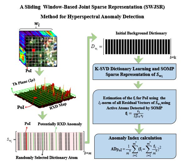
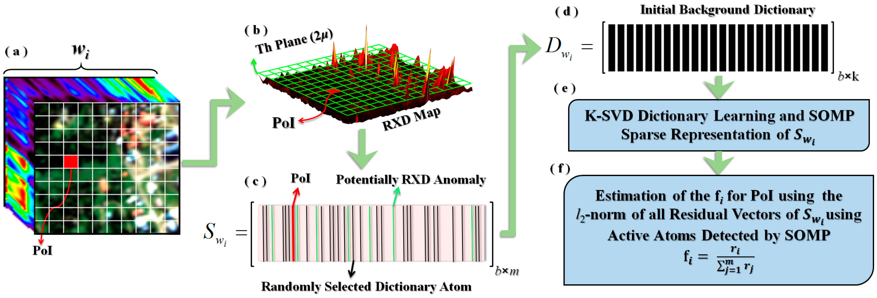
Simultaneous sparse representation of all pixels occurring in each wi using a unique set of local background atoms from a learned dictionary is the main idea of the proposed method in the field of anomaly index generation. Through this process, it is expected that simultaneous estimation of all the available signals in wi leads to imposing the selection of the descriptive background atoms. Consequently, the increase in the l2-norm of the estimated residuals for each signal could be interpreted as the level of anomaly. In this procedure, using the traditional RXD anomaly, the randomly selected signals used in dictionary learning are initially refined by exclusion of highly-probable anomaly signals. Figure 2 illustrates the process of fi estimation in a wi occurrence.
Here, a spatial subset of a hyperspectral image that coincided with the position of wi is depicted where the PoI inside the wi is shown as a red pixel (parts a, b, and c). Obviously the transition of wi will change the location of the PoI in it.
According to Figure 2, and as the first step, using the traditional RXD, the potentially anomalous signals were removed by applying a proper threshold (Th-Plane). This threshold is set to twice of the average (2μ) of RXD map. In continue, the signals having higher values than Th-Plane were omitted from randomly selection process of dictionary learning (parts c and d). The aim of this process is to perform initial refinement of dictionary atoms. Thus, the initial dictionary atoms (Dwi) would be more descriptive to model the background signals.
In Figure 2, the matrix [Swi]b×m (b is the number of hyperspectral image bands) contains the constructive signals of wi where the green columns are indications of possible anomaly signals that are detected using RXD. The black columns are randomly-chosen candidates as initial atoms in the process of dictionary learning (Dwi). The number of signals used in dictionary learning (K) is equivalent to the ‘q’ percentage of the Swi signals in the case of the omitted probably-anomalous signals. As a result, the matrix Dwi would be constructed from matrix Swi as the initial dictionary in the dictionary learning process (part d).
To optimize the initial atoms of Dwi, the K-SVD method [43] has been utilized where the OMP algorithm [41] is used for the sparse coding process of each signal (part e). In this method, the direction of each dictionary atom is updated in an iterative process. This method is composed of two main steps. In the first step, sparse coding of all input signals (Swi) is performed, and, in the second step, for each selected atom, a new direction is calculated using the signals coded by the selected atom. This new direction is estimated through the Singular Value Decomposition (SVD) method of a matrix composed of columnar vectors, indicating the residual of the affected signals. In the other words, the estimated residual vector of the signals is calculated by only the signals affected by that selected atom. In this process, while the selected atom is absent, through elimination of the effect of the selected atom, the residual vector of the estimated signals will be calculated. Finally, the b-dimensional eigenvector corresponds to the largest singular value will be chosen as the substitute direction of each selected atom. As can be seen in [43], dictionary learning is an iterative procedure, which includes two steps (1) sparse coding of the Swi signals, and (2) optimization of the direction of Dwi atoms.
After the Dwi was learned via K-SVD, finding a common subspace for all Swi signals is performed through the SOMP algorithm (part e). In this algorithm, the sparse coding of a set of signals is simultaneously carried out. This means that all of the Swi signals will be simultaneously estimated through the same subspace spanned by the atoms in the learned dictionary with the minimum dimension. Furthermore, the minimization of the l2-norm of estimated residuals should be satisfied. The aim of this process is choosing the background descriptive atoms to reconstruct the Swi signals. As discussed before, it is expected that, during this process, the background signals are estimated to be more precise than the rare and anomalous signals. When considering this expectation, after the estimation of the Swi residual vectors using SOMP, their l2-norm for all wi signals would be calculated as rj, j = 1, 2, …, m. To continue, the index fi for the PoI will be estimated by normalizing the ri corresponding the location of PoI in wi through the Equation (3):
Through the transition of wi (i = 1, 2, …, m) on PoI, a m-dimensional vector FPoI will be generated. Finally, its variance would be selected as the criterion of anomaly detector after the 3σ statistical test (Equation (4). In this equation, m* is the number of fi for each PoI after the blunder separation procedure by the 3σ test. The well-known 3σ test is a standard statistical test to remove blunders from the random variable sets (fi). In this procedure, by assuming the normal distribution of the random variables, using mean (μ) and the standard deviation (σ) of the fi elements, those samples that are located within the range of μ − 3σ < fi < μ + 3σ are known as inliers and the other samples outside this interval are considered to be outliers. Finally, the outlier samples are removed from the data set and the anomaly index (Equation (4)) is calculated for the remaining samples [44]:
The following pseudo-code represents the general process of the proposed algorithm (Algorithm 1).
| Algorithm 1. SWJSR Anomaly Detector Algorithm. |
| Input: HyperCube Size of wi (m) Output: Anomaly Map
|
4. Datasets and Pre-Processing
Three real and two synthetic datasets were used in this research. The first real dataset contains an urban and forestry region of Cook city in Minnesota, USA acquired by a Hymap hyperspectral sensor with 126 spectral bands ranging from 370–512 μm in 2006. This data is freely available to the public through the Rochester Institute of Technology (RIT) and includes several targets with known spatial and spectral characteristics. This data is considered as a reference for the evaluation of target and anomaly detection methods. Figure 3 shows this reference data and the location of spectral targets. The details of the spectral targets and their behavior can be studied in [45].
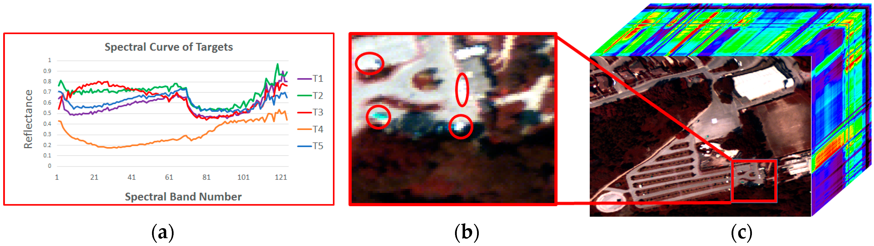
A subset of 80 × 100 pixels from the first real data containing six spectral targets was selected for analysis in this study. The second real data is from an airport zone of San Diego that has been collected by the AVIRIS sensor with 224 spectral bands ranging from 350–2510 nm. This has been converted to a 100 × 100 × 189 hypercube after removal of the water absorption and noisy bands. In this data, three spectral targets (airplanes) with extents of more than a couple of pixels exist and were used to apply the anomaly detection algorithms. Figure 4 displays the original data, the selected subset, and the spectral curve of the targets.
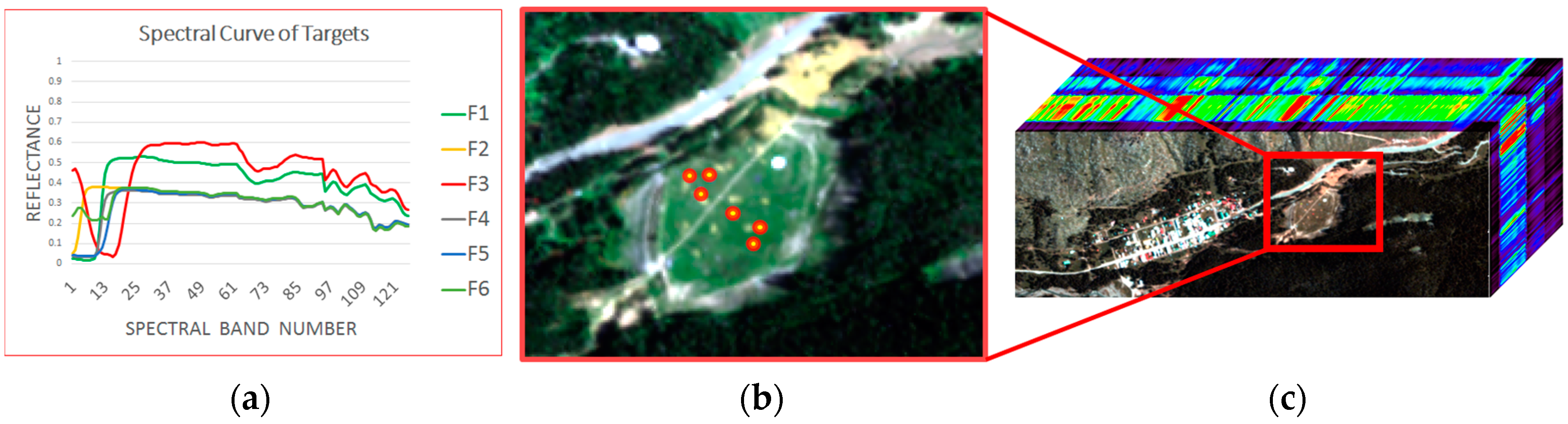
The third real data has been acquired from a region in Viareggio city in Italy collected by the SIM.GA airborne sensor [46]. Although this original dataset has 512 spectral bands, ranging from 388–994 nm, after removal of the low Signal to Noise Ratio (SNR) bands, by applying a spectral resampling process with a 4 nm interval, it has been converted to a 100 × 100 × 123 hypercube. In the area of interest on this image, five spectral targets with extents of more than a few pixels were chosen to apply anomaly detection algorithms. Figure 5 shows the original data, the area of interest, and the spectral curve of targets.
On the other hand, in the majority of previous works, the efficiency of the developed methods for target and anomaly detection has also been evaluated using synthetic data. In this research, two synthetic datasets were also created when considering two different strategies. As the first strategy, some sub-pixel targets were implanted in a region near to the location of the original targets from the Rochester Institute of Technology (RIT) data. Figure 6 shows the implantation targets and their spectral curves. Thus, this way, the number of spectral targets will be increased and a higher number of probable spectral anomalies should be identified. According to Figure 6, seven spectral targets with 50–80% of similarity to the original spectrum were linearly added to the hyperspectral image and a total of 13 potential anomaly pixels were constructed. Then, with the aim of simulating PSF effects, a Gaussian weighted averaging process using a 3 × 3 window around the location of the implanted target was applied.
As the second strategy of synthetic data generation, spectral destruction of original signals in the real RIT dataset was performed. In this strategy, a variation between ±5 to ±20% with respect to the original signals was applied to a randomly selected number of spectral bands (ranging from 5–10% of the total image bands) for six candidate pixels and a total of 12 potential anomaly pixels were constructed. The location of candidate pixels in this strategy were also locally chosen similar to the first strategy in the relatively homogeneous regions. The position of the destructed signals, a sample of the destructed spectral curve, and its related original data are displayed in Figure 7.
5. Results and Discussion
As mentioned before, to evaluate the results and efficiency of the proposed algorithm, five types of different data consisting of three real and two synthetic datasets were used.
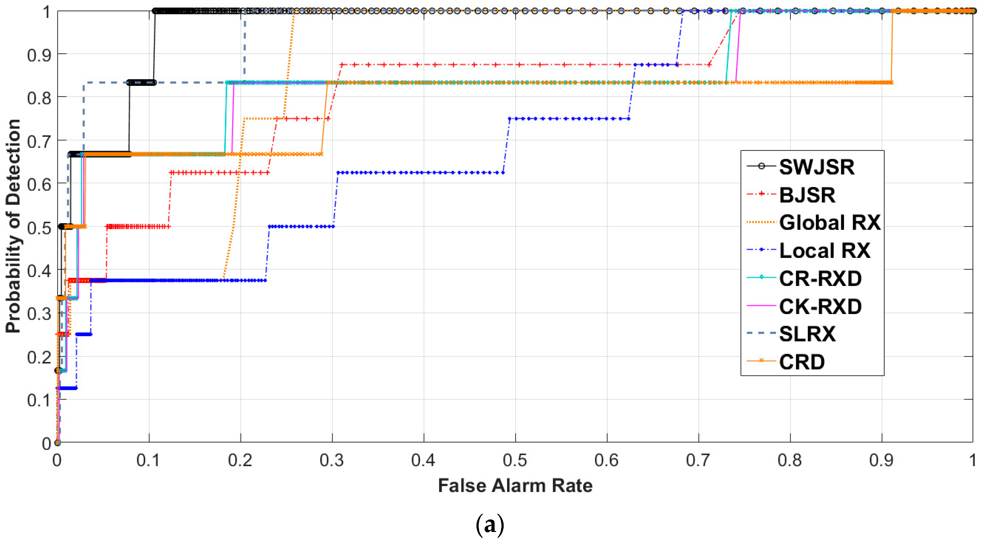
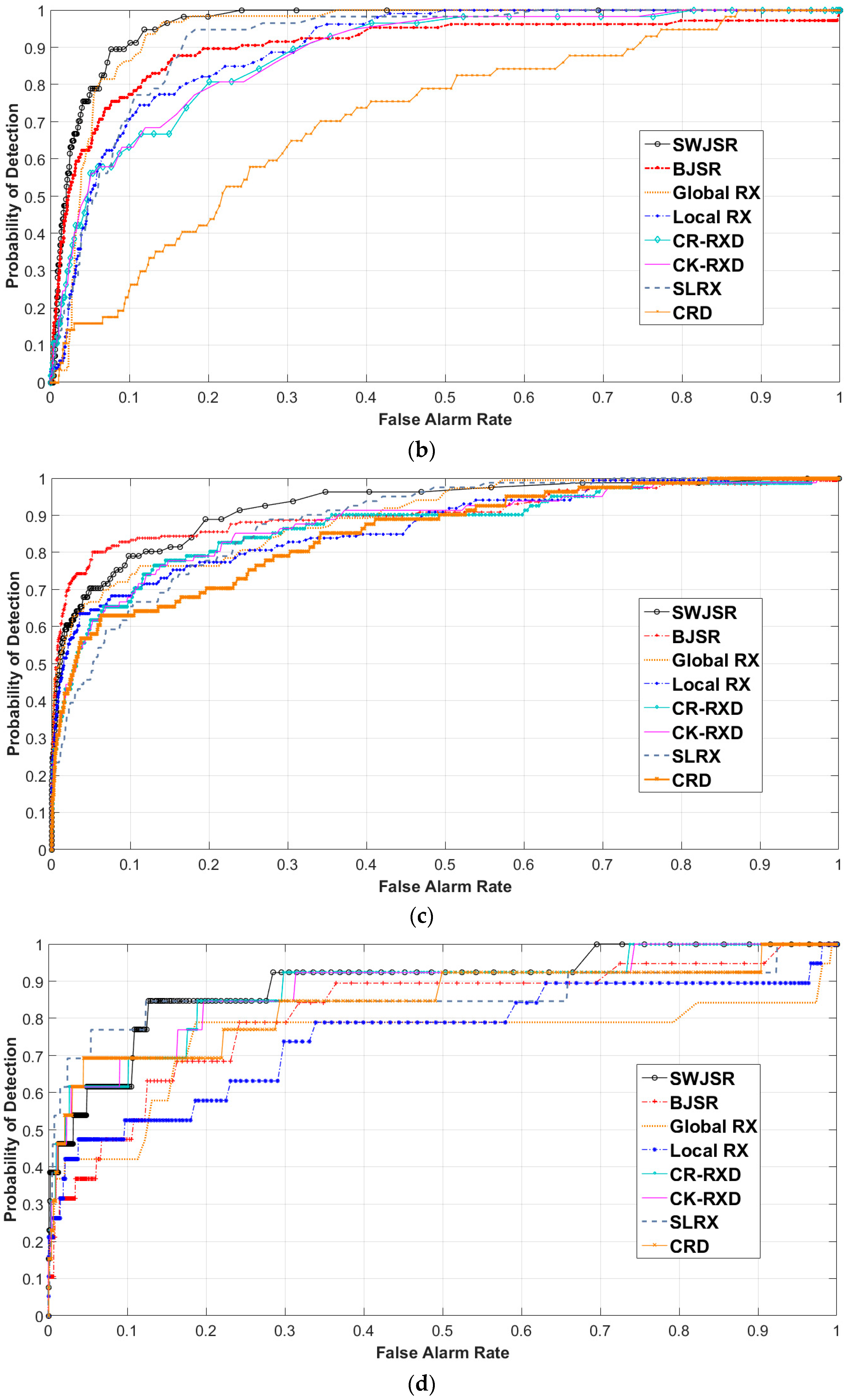
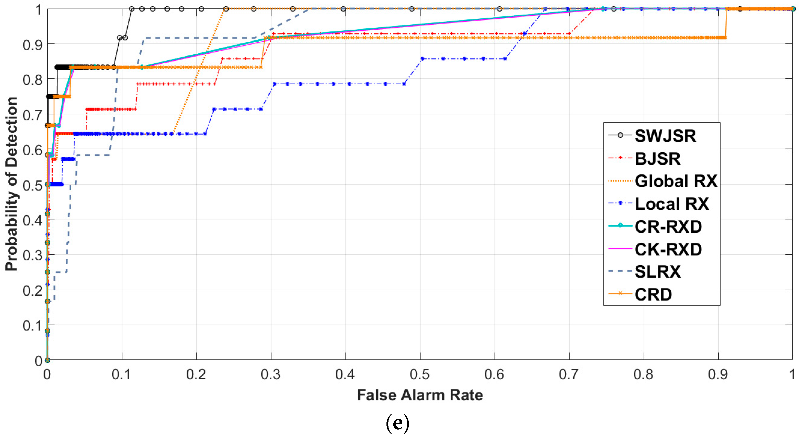
In this study, the functionality of the proposed method was assessed by performing the three-dimensional (3D)-ROC analysis [10,14] (Figure 8), evaluating the area under curves (Figure 9 and Table 1), background suppression criteria (Figure 10 and Table 1) and the generation of a target-background separation diagram [5] (Figure 11).
The traditional ROC curve is obtained by plotting of the false alarm rate (PFA (versus the correct probability of detection (PD (for different thresholds through Equation (5):
Since the output of anomaly detection algorithms is an image with two anomaly and background classes, by calculating the ratio of the number of correctly-detected anomaly pixels (NSignal detected) to the total anomaly pixels (Nt )for each threshold, the probability of correct detection is calculated. Additionally, with the calculation of the ratio of number of background pixels wrongly placed in the anomaly class (NFalse Alarm) to the all pixels of the image (N), the probability of wrong detection (known as the false alarm rate) for each threshold will be obtained.
Recently, the 3-D ROC analysis with some advantages respect to 2-D one was developed to evaluate anomaly detection algorithms [44]. In this case, varying the value of threshold (Th) enables the users to observe progressive changes in PD and PFA independently. A 3-D ROC curve can be generated when considering PD, PFA, and threshold (Th) as three components of a 3D point in the Cartesian coordinate system. In other words, it is a three-dimensional curve of (PD, PFA, Th), in which three different 2-D ROC curves could be also generated from each aspect. The 2-D ROC that was obtained from (PD, PFA) is the traditional one and the 2-D ROC obtained from (PFA, Th) or (PD, Th) are the new ones.
The 2-D ROC of (PD, Th) could be represented as the progressive detection power versus the changes of threshold and the 2-D ROC of (PFA, Th) provides important information of progressive background suppression as the threshold varies, especially in the case of visual interpretation with no availability of ground truth data.
Having obtained the detection maps of each method in different situations, the plot of this 3D curve for 5000 numbers of different thresholds with the minimum and maximum limit of the map of detection was performed and the area under curves were considered as a scale of the evaluation of the efficiency.
The separability diagram is also one of the indices of efficiency evaluation of two-class classification algorithms that shows the statistical separation of anomaly and background data. This diagram is generated with the help of the ground truth map and shows the range of the recorded values in the anomaly and background locations in the detection map. The level of separation or a presence of overlap among the domains of anomaly and background values indicate the level of success of the anomaly detection algorithm. In plotting this diagram, the following steps are considered: (1) generating anomaly detection maps for all of the compared methods; (2) normalization of detection maps considering the minimum and maximum of all anomaly detection maps simultaneously; (3) identification of anomaly and background signals through a ground truth reference map; and, (4) estimation of the minimum and maximum anomaly and background values for each detection map in two ways:
- (A)
- without removing any of the signals that lead to the drawing of the bars in the graphs; and,
- (B)
- removing 10% of the minimum and maximum values of background and anomaly signals and mapping down the dropped domain into colored boxes.
To compare the results obtained from the proposed algorithm, seven other anomaly detection algorithms were also implemented. The traditional Global and Local RX algorithms [12], Causal R-RX, and K-RX [22], as well as the recently-developed CRD [23] and BJSR [33] algorithms in the field of anomaly detection were chosen for this evaluations. Except the Global RX which has not any setting parameters, other six algorithms have several setting parameters. Generally, default setting parameters proposed by the developers were used in our comparisons. Window size is the only setting parameter in Local RX method. Generally, the best result obtained from windows of 11 × 11, 13 × 13 and 15 × 15 pixels were used in the comparisons. In Causal R-RX and K-RX, the window width of sliding array is the main setting parameter which set to CW = 900, according the best result obtained in [22]. The CRD setting are inner and outer windows as well as the regularization parameters. Here, a 7 × 7 inner and a 15 × 15 outer window size as well as 10−6 were set as the regularization parameter [23]. In continue, the BJSR setting parameters are background and guard window size, search window and level of sparsity. Window sizes (background and guard) were selected based on the optimum setting reported in [33]. So, a 17 × 17 background window, 5 × 5 guard window, and 19 × 19 search window were the spatial setting and the sparsity level was set to 3 in SOMP method [33]. However, among the detection algorithms used in this paper, the Local RX algorithm (LRX) was easily adapted to the proposed sliding window. Thus, a new version of Local RX called the Sliding-window Local RX anomaly detector (SLRX) is also used in the evaluations. In this version, the generation of FPOI for each PoI is based on the Mahalanobis distance calculated by the Local RX of samples in the wi windows. Again, and similar to the method of SWJSR, the variance of FPoI has been used as the measure of this detector for each PoI.
Table 1 presents the results of AUC index (PD, PFA, and PFA, Th) for the abovementioned algorithms and the best results by the proposed algorithm (SWJSR) implemented on the five types of real and synthetic data (implanted and destructed data).
When considering the traditional AUC (PD, PFA) that is provided in Table 1, in the similar conditions the higher efficiency of the proposed algorithm is observed. Thus, an average 2% improvement when compared to the best results obtained from the other methods is noticeable. On the other hand, the AUC (PFA, Th) values of the proposed method are rather lower than the other algorithms. It should be noted that the AUC of PFA vs. Th represents the level of background suppression and their lower values indicate the better performance of the algorithms [47]. In order to compare the anomaly detection algorithms, the 3D-ROC curves, 2-D ROCs of (PD, PFA), 2-D ROCs of (PFA, Th), and the target-background separation diagrams that are related to each dataset (Table 1) are shown in the following figures (Figure 8, Figure 9, Figure 10 and Figure 11).
Again, higher efficiency of the SWJSR algorithm can be seen from the formation mechanism of 3-D ROC curves and separability diagrams. These diagrams, except for the implanted synthetic data, also reveal the desirable separation between the anomaly and background elements in the proposed method, which is a verification of better functionality when compared to the other methods.
In the case of synthetic data, all of the compared methods yield similar results. In the case of ROC (PD, PF) curves, mainly for all of the applied examinations, the relevant curve of the SWJSR is closer to the upper-left of the diagram and this factor has yielded the increase of the AUC (PD, PF) value.
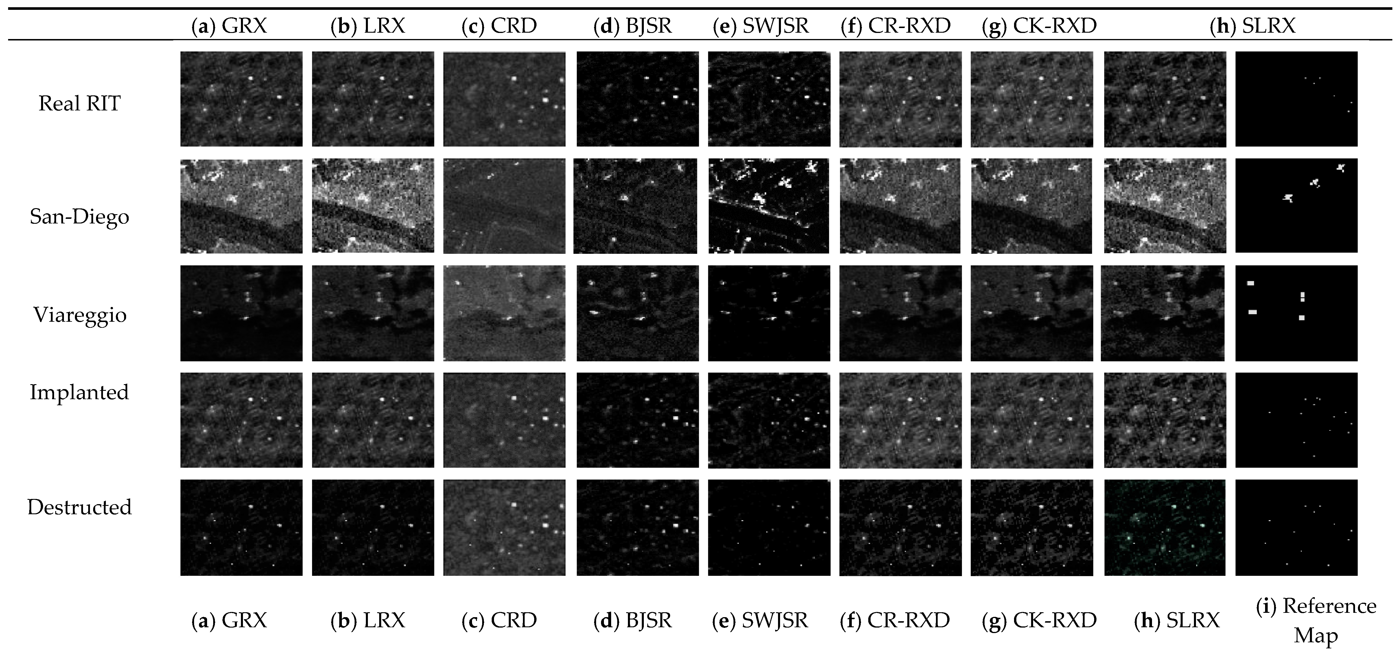
Figure 12 shows the obtained detection maps by the GRX, LRX, CRD, BJSR, CR-RXD, CK-RXD, SLRX, and the proposed algorithms (SWJSR) for the reference ground truth map and for all of the used data in this research.
According to the best obtained results from the suggested SWJSR algorithm, the sensitivity analysis of this algorithm with respect to its tuning parameters was also implemented. These parameters, including: (1) the dimensions of the sliding window; and, (2) the level of sparsity, were used in simultaneous reconstruction of the background signals by SOMP algorithm. As the first investigation, the results of changing the sliding window dimensions in the AUC index for all of the used data are presented in Table 2.
As shown in Table 2, the obtained results depend on the correct definition of the dimensions of the sliding window. In this regard, according to part b of Figure 2, using the traditional RXD, to remove potentially anomalous signals by applying a proper threshold (Th-Plane), the covariance matrix that was estimated from a small number of data samples, could involve rank-deficient (non-invertible) matrices. To overcome numerical instabilities in case of smaller sliding windows, the pseudo inverse based on the Moore-Penrose method was used. To this aim when the number of samples (sliding window elements) was less than the number of spectral bands, the “pinv” function was used as an alternative of common inversion function (inv) in MATLAB. In the case of spectral anomalies with large spatial extension, it is necessary to use large sliding windows to achieve better results. For example, since the multi-pixel anomaly regions for the San Diego airport zone and Viareggio city in Italy are more extended than one-pixel anomalies in the RIT data, the optimum sliding window is also larger. The same rule also applies to the San Diego data compared with the Viareggio data, and the larger sliding window dimensions are convenient. Thus, keeping this rule in mind and while considering the spatial resolution of the sensor, obtaining primary knowledge about the extension of probable anomalies could be effective in tuning the sliding window size, reaching reliable results faster. This knowledge is less important when dealing with anomalies in the range of one pixel or less.
One of the most important tuning parameters of the suggested algorithm is a determination of the level of simultaneous sparse estimation of the background elements, which is called level of sparsity. In other words, the maximum number of atoms used from the learned dictionary for simultaneous estimation of all signals located in the sliding window is another tuning parameter. It is obvious that the value of this parameter depends on the variety of the occurrence of endmembers in the window. Since this value is indicative of the maximum use of the dictionary atoms, it is obvious that a lower, or the same, number of dictionary atoms that are proportional to this tuning parameter are selected in the recovery of all sliding window positions. Assigning a low number for this parameter yields an incomplete modeling of the background, and, when considering a higher number than necessary, results in the possibility of cooperation of unrelated atoms in decreasing the recovery residuals during the anomaly occurrence. Accordingly, the optimum value of this parameter was selected in a way that provided a balance between the two mentioned boundaries of the consequences of the incorrect selection of this parameter.
In Table 3, by assigning the identified optimum value for each dataset to the dimension of the sliding window, the effect of changing the level of sparsity in the AUC index has also been studied for all the datasets.
As observed from the results of Table 3, an optimized selection of this parameter has a significant role in the efficiency of the proposed algorithm. Indeed, considering the variety of the input data, choosing values of 5, 6, or 7 for this parameter will mainly yield desirable results, although in the ranges close to the optimum value this parameter did not reveal a significant change in results. Incorrect determination of this will considerably influence the results.
Since the proposed method involves considerably high processing when compared to other methods, it could not be compared from the computational cost and running time point of view. For example, the running time for RIT data in MATLAB software using a computer having an Intel Core i7 2.6 GHz processor and 16 GB of RAM under the Windows 10 64-bit operating system was 129 s, which is longer than the other methods. Nevertheless, the average running time of the proposed method in comparison with other methods are tabulated in Table 4. These times are the average value of running times of all datasets in each anomaly detection algorithm.
Finally, it seems that utilizing and developing parallel processing systems will increase the speed of running the proposed algorithm that is the focus of future studies of the authors.
6. Conclusions
Since the development of anomaly detection algorithms for hyperspectral images includes a large number of applications, many researchers are motivated to develop efficient methods in this area. In this paper, a new method based on simultaneous sparse representation of local background signals using a sliding window was proposed to detect spectral anomalies. In this method, all of the signals located in the sliding window are voted through examining the estimated error of each signal to determine if there is any anomaly or not. As the precision of recovery for each pixel of the hyperspectral image is evaluated several times during the transition of the sliding window, this potential provides better conditions for evaluation of each signal from being an anomaly or background. The learned dictionary in each position of the sliding window is affected by the signals that are located in that window, and, practically, each pixel is being recovered many times with the help of a set of different background dictionaries.
The results of implementation of the proposed SWJSR method in five used datasets in this research proved its higher functionality when compared to the GRX, LRX, CRD, BJSR, CR-RXD, CK-RXD, and SLRX detectors. According to the obtained AUC, the results show the average improvement of efficiency (AUC) of about 7.5%, 14.25%, 8.2%, 8.25%, 6.45%, 6.5%, and 3.6%, respectively, in comparison to the mentioned algorithms. The implementation of this idea and its success showed that development of voting algorithms and the combination of the results could be considered as an effective approach to detect anomalies in hyperspectral signals. This idea could also be utilized in other hyperspectral image processing algorithms to evaluate the results by comparing prior methods. The results of SLRX, which show the average improvement of efficiency (AUC) of about 10% in comparison with traditional local RX, confirms this idea.
Automatic tuning of the proposed SWJSR algorithm parameters and developing parallel processing techniques to improve the running time of this algorithm are the focus of future research of the authors. Moreover, detecting spatial anomalies by the proposed approach and using spatial-spectral features in this field include other interested future works of the authors.
Acknowledgments
The authors would like to thank the Center for Imaging Science, Rochester Institute of Technology for the “HyMap” data set and also the Remote Sensing & Image Processing Group of University of Pisa for the “Viareggio 2013 Trial” data set used in our experiments to evaluate the proposed anomaly detection algorithm.
Author Contributions
All the authors listed contributed equally to the work presented in this paper.
Conflicts of Interest
The authors declare no conflict of interest.
References
- Landgrebe, D. On Information Extraction Principles for Hyperspectral Data; School of Electrical and Computer Engineering, Purdue University: West Lafayette, IN, USA, 1997; pp. 168–173. [Google Scholar]
- Shaw, G.; Manolakis, D. Signal Processing for Hyperspectral Image Exploitation. IEEE Signal Process. Mag. 2002, 19, 12–16. [Google Scholar] [CrossRef]
- Chang, C.-I. Hyperspectral Imaging: Techniques for Spectral Detection and Classification; Kluwer Academic/Plenum Publishers: New York, NY, USA, 2003; ISBN 0-306-47483-2. [Google Scholar]
- Matteoli, S.; Diani, M.; Corsini, G. A tutorial overview of anomaly detection in hyperspectral images. IEEE Aerosp. Electron. Syst. Mag. 2010, 25, 5–28. [Google Scholar] [CrossRef]
- Nasrabadi, N.M. Hyperspectral Target Detection: An overview of current and future challenges. IEEE Signal Process. Mag. 2014, 31, 34–44. [Google Scholar] [CrossRef]
- Sodemann, A.A.; Ross, M.P.; Borghetti, B.J. A Review of Anomaly Detection in Automated Surveillance. IEEE Trans. Syst. Man Cybern. Part C Appl. Rev. 2012, 42, 1257–1272. [Google Scholar] [CrossRef]
- Acito, N.; Diani, M.; Corsini, G. Gaussian mixture model based approach to anomaly detection in multi/hyperspectral images. In Proceedings of the SPIE Remote Sensing, Bruges, Belgium, 19–22 September 2005; Volume 5982, pp. 209–217. [Google Scholar]
- Eismann, M.T.; Stocker, A.D.; Nasrabadi, N.M. Automated hyperspectral cueing for civilian search and rescue. Proc. IEEE 2009, 97, 1031–1055. [Google Scholar] [CrossRef]
- Yuen, P.W.T.; Bishop, G. Hyperspectral Algorithm Development for Military Applications: A Multiple Fusion Approach. In Proceedings of the 3rd EMRS DTC Technical Conference, Edinburgh, UK, 13–14 July 2006. [Google Scholar]
- Chang, C.-I. Hyperspectral Data Processing: Algorithm Design and Analysis; Wiley: Hoboken, NJ, USA, 2013. [Google Scholar]
- Zhao, C.; Wang, Y.; Qi, B.; Wang, J. Global and local real-time anomaly detectors for hyperspectral remote sensing imagery. Remote Sens. 2015, 7, 3966–3985. [Google Scholar] [CrossRef]
- Reed, I.S.; Yu, X. Adaptive multiple-band CFAR detection of an optical pattern with unknown spectral distribution. IEEE Trans. Acoust. Speech Signal Process. 1990, 38, 1760–1770. [Google Scholar] [CrossRef]
- Chang, C.-I.; Chiang, S.-S. Anomaly Detection and Classification for Hyperspectral Imagery. IEEE Trans. Geosci. Remote Sens. 2002, 40, 1314–1325. [Google Scholar] [CrossRef]
- Chang, C.-I. Multiple-parameter receiver operating characteristic analysis for signal detection and classification. IEEE Sens. J. 2010, 10, 423–442. [Google Scholar] [CrossRef]
- Ren, H.; Chen, C.-W.; Chen, H.-T. Weighted anomaly detection for hyperspectral remotely sensed images. Proc. SPIE 2005, 5995, 63–68. [Google Scholar]
- Chang, C.-I.; Hsueh, M. Characterization of anomaly detection in hyperspectral imagery. Sens. Rev. 2006, 26, 137–146. [Google Scholar] [CrossRef]
- Kwon, H.; Nasrabadi, N.M. Kernel RX-Algorithm: A Nonlinear Anomaly Detector for Hyperspectral Imagery. IEEE Trans. Geosci. Remote Sens. 2005, 43, 388–397. [Google Scholar] [CrossRef]
- Kwon, H.; Der, S.Z.; Nasrabadi, N.M. Dual-window-based anomaly detection for hyperspectral imagery. Proc. SPIE 2003, 5094, 148–158. [Google Scholar]
- Kwon, H.; Der, S.Z.; Nasrabadi, N.M. Projection-Based Adaptive Anomaly Detection for Hyperspectral Imagery. In Proceedings of the 2003 International Conference on Image Processing (ICIP 2003), Barcelona, Spain, 14–17 September 2003; Volume 1. [Google Scholar]
- Liu, W.; Chang, C.I. A nested spatial window-based approach to target detection for hyperspectral imagery. In Proceedings of the IEEE International Geoscience and Remote Sensing Symposium (IGARSS), Anchorage, AK, USA, 20–24 September 2004; Volume 1, pp. 20–24. [Google Scholar]
- Liu, W.; Chang, C.-I. Multiple window anomaly detection for hyperspectral imagery. IEEE J. Sel. Top. Appl. Earth Obs. Remote Sens. 2013, 6, 644–658. [Google Scholar] [CrossRef]
- Chang, C.-I.; Wang, Y.; Chen, S.Y. Anomaly detection using causal sliding windows. IEEE J. Sel. Top. Appl. Earth Obs. Remote Sens. 2015, 8, 3260–3270. [Google Scholar] [CrossRef]
- Li, W.; Du, Q. Collaborative Representation for Hyperspectral Anomaly Detection. IEEE Trans. Geosci. Remote Sens. 2015, 53, 1463–1474. [Google Scholar] [CrossRef]
- Yuan, Y.; Wang, Q.; Zhu, G. Fast Hyperspectral Anomaly Detection via High-Order 2D Crossing Filter. IEEE Trans. Geosci. Remote Sens. 2015, 53, 620–630. [Google Scholar] [CrossRef]
- Yuan, Y.; Ma, D.; Wang, Q. Hyperspectral Anomaly Detection by Graph Pixel Selection. IEEE Trans. Cybern. 2016, 46, 3123–3134. [Google Scholar] [CrossRef] [PubMed]
- Bruckstein, A.M.; Donoho, D.L.; Elad, A. From sparse solutions of systems of equations to sparse modeling of signals and images. SIAM Rev. 2009, 51, 34–81. [Google Scholar] [CrossRef]
- Willett, R.M.; Duarte, M.F.; Davenport, M.A.; Baraniuk, R.G. Sparsity and Structure in Hyperspectral Imaging. IEEE Signal Process. Mag. 2014, 31, 116–126. [Google Scholar] [CrossRef]
- Chen, Y.; Nasrabadi, N.M.; Tran, T.D. Simultaneous joint sparsity model for target detection in hyperspectral imagery. IEEE Geosci. Remote Sens. Lett. 2011, 8, 676–680. [Google Scholar] [CrossRef]
- Du, B.; Zhang, Y.; Zhang, L.; Tao, D. Beyond the Sparsity-Based Target Detector: A Hybrid Sparsity and Statistics-Based Detector for Hyperspectral Images. IEEE Trans. Image Process. 2016, 25, 5345–5357. [Google Scholar] [CrossRef] [PubMed]
- Zhang, Y.; Du, B.; Zhang, L. A sparse representation-based binary hypothesis model for target detection in hyperspectral images. IEEE Trans. Geosci. Remote Sens. 2015, 53, 1346–1354. [Google Scholar] [CrossRef]
- Li, F.; Zhang, Y.; Zhang, L.; Zhang, X.; Jiang, D. Hyperspectral anomaly detection using background learning and structured sparse representation. In Proceedings of the IEEE International Geoscience and Remote Sensing Symposium (IGARSS), Beijing, China, 10–15 July 2016. [Google Scholar]
- Yuan, Z.; Sun, H.; Ji, K.; Li, Z.; Zou, H. Local sparsity divergence for hyperspectral anomaly detection. IEEE Geosci. Remote Sens. Lett. 2014, 11, 1697–1701. [Google Scholar] [CrossRef]
- Li, J.; Zhang, H.; Zhang, L.; Ma, L. Hyperspectral anomaly detection by the use of background joint sparse representation. IEEE J. Sel. Top. Appl. Earth Obs. Remote Sens. 2015, 8, 2523–2533. [Google Scholar] [CrossRef]
- Zhao, R.; Du, B.; Zhang, L. Hyperspectral Anomaly Detection via a Sparsity Score Estimation Framework. IEEE Trans. Geosci. Remote Sens. 2017, 55, 3208–3222. [Google Scholar] [CrossRef]
- Zhang, L.; Zhao, C. Hyperspectral anomaly detection based on spectral-spatial background joint sparse representation. Eur. J. Remote Sens. 2017, 50, 362–376. [Google Scholar] [CrossRef]
- Ma, D.; Yuan, Y.; Wang, Q. A Sparse Dictionary learning method for Hyperspectral Anomaly Detection with Capped Norm. In Proceeding of the IEEE International Geoscience and Remote Sensing Symposium (IGARSS), Fort Worth, TX, USA, 23–28 July 2017; pp. 648–651. [Google Scholar]
- Chen, Y.; Nasrabadi, N.M.; Tran, T.D. Sparse representation for target detection in hyperspectral imagery. IEEE J. Sel. Top. Signal Process. 2011, 5, 629–640. [Google Scholar] [CrossRef]
- Tropp, J.A.; Wright, S.J. Computational methods for sparse solution of linear inverse problems. Proceed. IEEE 2010, 98, 948–958. [Google Scholar] [CrossRef]
- Cotter, S.F.; Rao, B.D.; Engan, K.; Kreutz-Delgado, K. Sparse solutions to linear inverse problems with multiple measurement vectors. IEEE Trans. Signal Process. 2005, 53, 2477–2488. [Google Scholar] [CrossRef]
- Tropp, J.; Gilbert, A. Signal recovery from random measurements via orthogonal matching pursuit. IEEE Trans. Inf. Theory 2007, 53, 4655–4666. [Google Scholar] [CrossRef]
- Tropp, J.A.; Gilbert, A.C.; Strauss, M.J. Algorithms for simultaneous sparse approximation. Part I: Greedy pursuit. Signal Process. 2006, 86, 572–588. [Google Scholar] [CrossRef]
- Aravind, N.V.; Abhinandan, K.; Acharya, V.V.; Sumam, D.S. Comparison of OMP and SOMP in the reconstruction of compressively sensed hyperspectral images. In Proceedings of the International Conference on Communications and Signal Processing (ICCSP), Calicut, India, 10–12 February 2011; pp. 188–192. [Google Scholar]
- Aharon, M.; Elad, M.; Bruckstein, A. K-SVD: An algorithm for designing over-complete dictionaries for sparse representation. IEEE Trans. Signal Process. 2006, 54, 4311–4322. [Google Scholar] [CrossRef]
- Mikhail, E.M.; Ackermann, F. Observations and Least Squares; IEP: New York, NY, USA, 1976. [Google Scholar]
- Target Detection Blind Test. Available online: http://dirsapps.cis.rit.edu/blindtest/ (accessed on 26 February 2018).
- Acito, N.; Matteoli, S.; Rossi, A.; Diani, M.; Corsini, G. Hyperspectral Airborne “Viareggio 2013 Trial” Data Collection for Detection Algorithm Assessment. IEEE J. Sel. Top. Appl. Earth Obs. Remote Sens. 2016, 9, 2365–2376. [Google Scholar] [CrossRef]
- Chang, C.-I. Real-Time Progressive Hyperspectral Image Processing: Endmember Finding and Anomaly Detection; Springer: Berlin, Germany, 2016; Part II, Chapters 5; pp. 14–18. [Google Scholar]
Figure 1.
Structure of moving the sliding window around the PoI.

Figure 2.
The process of the proposed anomaly detection algorithm.

Figure 3.
Rochester Institute of Technology (RIT) real dataset: (a) the spectral curve of targets; (b) the location of targets in selected subset; and, (c) original data.
Figure 3.
Rochester Institute of Technology (RIT) real dataset: (a) the spectral curve of targets; (b) the location of targets in selected subset; and, (c) original data.

Figure 4.
San Diego real dataset: (a) the spectral curve of targets; (b) the location of targets in selected subset; and, (c) the original data.
Figure 4.
San Diego real dataset: (a) the spectral curve of targets; (b) the location of targets in selected subset; and, (c) the original data.

Figure 5.
Viareggio real dataset: (a) the spectral curve of targets; (b) The location of targets in selected subset; and, (c) the original data.
Figure 5.
Viareggio real dataset: (a) the spectral curve of targets; (b) The location of targets in selected subset; and, (c) the original data.

Figure 6.
Implanted RIT dataset: (a) the spectral curve of implanted targets; (b) the location of implanted targets in selected subset; and, (c) the original data.
Figure 6.
Implanted RIT dataset: (a) the spectral curve of implanted targets; (b) the location of implanted targets in selected subset; and, (c) the original data.

Figure 7.
Destructed RIT dataset: (a) the spectral curve of destructed targets; (b) the location of destructed targets in the selected subset; and, (c) the original data.
Figure 7.
Destructed RIT dataset: (a) the spectral curve of destructed targets; (b) the location of destructed targets in the selected subset; and, (c) the original data.

Figure 8.
3D ROC curves of the anomaly detection algorithms: (a) Real RIT dataset; (b) Real San Diego dataset; (c) Real Viareggio dataset; (d) Implanted RIT dataset; and, (e) Destructed RIT dataset.
Figure 8.
3D ROC curves of the anomaly detection algorithms: (a) Real RIT dataset; (b) Real San Diego dataset; (c) Real Viareggio dataset; (d) Implanted RIT dataset; and, (e) Destructed RIT dataset.


Figure 9.
2-D ROC (PD, PF) of the anomaly detection algorithms: (a) Real RIT dataset; (b) Real San Diego dataset; (c) Real Viareggio dataset; (d) Implanted RIT dataset; and, (e) Destructed RIT dataset.
Figure 9.
2-D ROC (PD, PF) of the anomaly detection algorithms: (a) Real RIT dataset; (b) Real San Diego dataset; (c) Real Viareggio dataset; (d) Implanted RIT dataset; and, (e) Destructed RIT dataset.


Figure 10.
2-D ROC (PF,Th) of the anomaly detection algorithms: (a) real RIT dataset; (b) real San Diego dataset; (c) real Viareggio dataset; (d) implanted RIT dataset; and, (e) destructed RIT dataset.
Figure 10.
2-D ROC (PF,Th) of the anomaly detection algorithms: (a) real RIT dataset; (b) real San Diego dataset; (c) real Viareggio dataset; (d) implanted RIT dataset; and, (e) destructed RIT dataset.


Figure 11.
Target-background separation diagram of the anomaly detection algorithms (the green box shows the target and the red box shows background statistics): (a) real RIT dataset; (b) real San Diego dataset; (c) real Viareggio dataset; (d) implanted RIT dataset; and, (e) destructed RIT dataset.
Figure 11.
Target-background separation diagram of the anomaly detection algorithms (the green box shows the target and the red box shows background statistics): (a) real RIT dataset; (b) real San Diego dataset; (c) real Viareggio dataset; (d) implanted RIT dataset; and, (e) destructed RIT dataset.


Figure 12.
Detection maps of compared algorithms for all datasets: (a) GRX detection map; (b) LRX detection map; (c) CRD detection map; (d) Background Joint Sparse Representation (BJSR) detection map; (e) SWJSR detection map; (f) CR-RXD detection map; (g) CK-RXD detection map. (h) SLRX detection map; and, (i) Reference anomaly map.


Table 1.
Average improvement of efficiency (AUC) of the GRX, local RX algorithm (LRX), CRD, BJSR, CR-RXD, CK-RXD, sliding-window Local RX anomaly detector (SLRX), and SWJSR for all the datasets. (The bold one is higher in case of AUC(PD, PFA) and it is lower in case of AUC(PFA, Th)).
Table 1.
Average improvement of efficiency (AUC) of the GRX, local RX algorithm (LRX), CRD, BJSR, CR-RXD, CK-RXD, sliding-window Local RX anomaly detector (SLRX), and SWJSR for all the datasets. (The bold one is higher in case of AUC(PD, PFA) and it is lower in case of AUC(PFA, Th)).
| Algorithm | GRX | LRX | CRD | BJSR | CR-RXD | CK-RXD | SLRX | SWJSR | |
|---|---|---|---|---|---|---|---|---|---|
| Dataset | |||||||||
| Real RIT | AUC(PD, PFA) | 0.8619 | 0.7014 | 0.7935 | 0.8179 | 0.8372 | 0.8334 | 0.9563 | 0.9668 |
| AUC(PFA, Th) | 0.0357 | 0.1524 | 0.0487 | 0.0082 | 0.0355 | 0.0363 | 0.1988 | 0.0137 | |
| Real San Diego | AUC(PD, PFA) | 0.9471 | 0.8984 | 0.7078 | 0.9050 | 0.8822 | 0.8832 | 0.9165 | 0.9638 |
| AUC(PFA, Th) | 0.0417 | 0.0585 | 0.0544 | 0.0133 | 0.0038 | 0.0037 | 0.0039 | 0.0017 | |
| Real Viareggio | AUC(PD, PFA) | 0.8774 | 0.8433 | 0.8521 | 0.9128 | 0.8732 | 0.8773 | 0.8849 | 0.9242 |
| AUC(PFA, Th) | 0.1189 | 0.0590 | 0.0755 | 0.0227 | 0.0482 | 0.0440 | 0.0159 | 0.0022 | |
| Implanted RIT | AUC(PD, PFA) | 0.7425 | 0.7404 | 0.8433 | 0.7834 | 0.8792 | 0.8783 | 0.8598 | 0.8922 |
| AUC(PFA, Th) | 0.0323 | 0.0887 | 0.0486 | 0.0179 | 0.0354 | 0.0362 | 0.0782 | 0.0084 | |
| Destructed RIT | AUC(PD, PFA) | 0.9264 | 0.8326 | 0.8961 | 0.8968 | 0.9340 | 0.9320 | 0.9294 | 0.9818 |
| AUC(PFA, Th) | 0.0075 | 0.0426 | 0.0431 | 0.0180 | 0.0010 | 0.0011 | 0.0021 | 0.0015 |
Table 2.
Effect of size of sliding window in the Sliding Window-Based Joint Sparse Representation (SWJSR) detector for all datasets. (The bold one is the higher).
Table 2.
Effect of size of sliding window in the Sliding Window-Based Joint Sparse Representation (SWJSR) detector for all datasets. (The bold one is the higher).
| Size of Window | SW = 8 | SW = 9 | SW = 10 | SW = 11 | SW = 12 | SW = 13 | SW = 14 | SW = 15 | SW = 17 | SW = 20 | Average | Standard Deviation | |
|---|---|---|---|---|---|---|---|---|---|---|---|---|---|
| Dataset | |||||||||||||
| Real RIT | AUC | 0.9216 | 0.8937 | 0.9668 | 0.9603 | 0.9459 | 0.9273 | 0.9182 | 0.8839 | 0.878 | 0.8435 | 0.9139 | 0.0391 |
| Real San Diego | AUC | 0.8743 | 0.8912 | 0.9125 | 0.9420 | 0.9470 | 0.9570 | 0.9548 | 0.9638 | 0.9614 | 0.9690 | 0.937 | 0.0330 |
| Real Viareggio | AUC | 0.8736 | 0.8749 | 0.8775 | 0.8780 | 0.8832 | 0.8739 | 0.9099 | 0.9127 | 0.9242 | 0.911 | 0.8919 | 0.0199 |
| Implanted RIT | AUC | 0.8849 | 0.8740 | 0.8922 | 0.8829 | 0.8641 | 0.8625 | 0.8390 | 0.8376 | 0.8189 | 0.7996 | 0.8556 | 0.0307 |
| Destructed RIT | AUC | 0.9639 | 0.9475 | 0.9818 | 0.9784 | 0.9767 | 0.9629 | 0.9604 | 0.9501 | 0.9369 | 0.9140 | 0.9573 | 0.0198 |
Table 3.
Effect of the level of sparsity in the SWJSR detector for all datasets. (The bold one is the higher).
Table 3.
Effect of the level of sparsity in the SWJSR detector for all datasets. (The bold one is the higher).
| Level of Sparsity | 2 | 3 | 4 | 5 | 6 | 7 | 8 | Average | Standard Deviation | |
|---|---|---|---|---|---|---|---|---|---|---|
| Dataset | ||||||||||
| Real RIT | AUC | 0.6352 | 0.8226 | 0.8993 | 0.9434 | 0.9673 | 0.9668 | 0.9607 | 0.8850 | 0.1219 |
| Real San Diego | AUC | 0.9196 | 0.9303 | 0.9499 | 0.9615 | 0.9638 | 0.9602 | 0.9620 | 0.9496 | 0.0177 |
| Real Viareggio | AUC | 0.8467 | 0.9126 | 0.9265 | 0.9307 | 0.9127 | 0.9115 | 0.9060 | 0.9066 | 0.0279 |
| Implanted RIT | AUC | 0.5796 | 0.7382 | 0.8414 | 0.8668 | 0.8922 | 0.9115 | 0.9103 | 0.82 | 0.1217 |
| Destructed RIT | AUC | 0.7500 | 0.8947 | 0.9442 | 0.9733 | 0.9818 | 0.9802 | 0.9811 | 0.9293 | 0.0852 |
Table 4.
Average running time of the compared algorithms using all datasets.
| Algorithm | GRX | LRX | CRD | BJSR | CR-RXD | CK-RXD | SLRX | SWJSR |
|---|---|---|---|---|---|---|---|---|
| Running Time (s) | 2.05 | 22.74 | 33.28 | 51.48 | 8.27 | 9.62 | 102.51 | 193.14 |
© 2018 by the authors. Licensee MDPI, Basel, Switzerland. This article is an open access article distributed under the terms and conditions of the Creative Commons Attribution (CC BY) license (http://creativecommons.org/licenses/by/4.0/).
Share and Cite
MDPI and ACS Style
Soofbaf, S.R.; Sahebi, M.R.; Mojaradi, B. A Sliding Window-Based Joint Sparse Representation (SWJSR) Method for Hyperspectral Anomaly Detection. Remote Sens. 2018, 10, 434. https://doi.org/10.3390/rs10030434
AMA Style
Soofbaf SR, Sahebi MR, Mojaradi B. A Sliding Window-Based Joint Sparse Representation (SWJSR) Method for Hyperspectral Anomaly Detection. Remote Sensing. 2018; 10(3):434. https://doi.org/10.3390/rs10030434
Chicago/Turabian StyleSoofbaf, Seyyed Reza, Mahmod Reza Sahebi, and Barat Mojaradi. 2018. "A Sliding Window-Based Joint Sparse Representation (SWJSR) Method for Hyperspectral Anomaly Detection" Remote Sensing 10, no. 3: 434. https://doi.org/10.3390/rs10030434
Note that from the first issue of 2016, this journal uses article numbers instead of page numbers. See further details here.