A Topography-Informed Morphology Approach for Automatic Identification of Forest Gaps Critical to the Release of Avalanches

Department of Environmental Systems Science, ETH Zurich, 8092 Zurich, Switzerland
*
Author to whom correspondence should be addressed.
Remote Sens. 2018, 10(3), 433; https://doi.org/10.3390/rs10030433
Submission received: 19 December 2017
/
Revised: 2 March 2018
/
Accepted: 4 March 2018
/
Published: 10 March 2018
(This article belongs to the Special Issue Lidar for Forest Science and Management)
Abstract
:Human assets in Alpine regions are prone to gravitational natural hazards such as rock fall, shallow landslides and avalanches. Forests make up a substantial share in that landscape and can mitigate those hazards. Management of avalanche protection forests must cope with avalanches potentially released in forest gaps, which can damage downslope forests. The Swiss guidelines “Sustainability and success monitoring in protection forests” prescribe forest-gap extents in slope-line direction critical to the release of avalanches in forested areas. This article proposes a topography-informed morphology approach (TIMA) to automate the detection of critical gaps based on a digital terrain model and a canopy height model (CHM) derived from airborne LiDAR-data. TIMA uses complementary information about topography to probe forest gaps computed from the CHM with templates meeting critical-gap extents adjusted to local topography. The method was applied to a test site in Klosters-Serneus (Switzerland). The comparison of a critical-gap map with the results of a field assessment at 19 sample locations resulted in 84% overall accuracy. Moreover, plausibility of gap detection could be improved by including linear features forest roads and torrent channels in TIMA to account for decoupled snow layer resulting from abrupt breaks on the hillslope. If the TIMA concept can be successfully applied to the case of avalanches, this would encourage its use in assessing other gravitational natural hazard processes.
1. Introduction
1.1. Context and Problem
Densely populated Alpine regions as encountered in Austria, France, Italy and Switzerland are prone to gravitational natural hazard processes such as rockfall, shallow landslides and avalanches as the consequence of the steep topographical relief. Often forming a substantial share in these landscapes, forests play an important role in making these regions habitable. Forests interact with these processes and mitigate their occurrence, magnitude or reach [1]. Around 5860 km of the Swiss forest (or 49% of the Swiss forest cover) have been identified as protection forests, i.e., forests mitigating processes on sites where human assets are at risk [2]. One-fifth (or, 1230 km) of all protection forests mitigate the occurrence of snow avalanches. The release of avalanches usually occurs on steep hillslopes ranging from 25 to 55° [3] because shear stress is too low for avalanches to occur on shallower hillslopes, and the snow layer constantly skids down on steeper hillslopes. Forests can effectively reduce the release of avalanches on these hillslopes when site conditions allow for growth of a sufficient forest canopy [3,4]. Forest-snow interactions are manifold: interception with tree crowns reduces the amount of snow deposed on forest floors, snow falling from the branches disturbs the formation of homogenous snow layers prone to releasement, and tree stems support the fixation of the snowpack [5].
Protection forests are a cheap and effective measure to protect against avalanches [6] and are managed to create and maintain a forest pattern which sustainably prevents the release of avalanches. Management guidelines have been developed in various countries to manage forests in potential avalanche release areas. Guidelines developed in Europe focus on the forest’s protection service [5,7,8,9,10] whereas a Canadian guideline focuses on reducing negative effects from clearcuts in forests used for wood production [11]. Gravity being the driving force behind avalanche hazard, all the guidelines put emphasis on the assessment of forest gaps in the slope-line, often relating critical-gap lengths to hillslope steepness [5,8,9,10,11]. These gaps can become release areas of avalanches, which can destroy the downslope forest. Moreover, the guidelines make specifications about forest structure (e.g., tree size, canopy coverage, basal area) presumed to be effective against the release of avalanches. The guidelines “Sustainability and success monitoring in protection forests” [5] are the Swiss quality standard for the management of forests protecting communities from gravity-driven natural hazards. Table 1 depicts critical-gap lengths in slope-line direction for the release of avalanches as proposed by the guidelines. The critical-gap length shrinks with increasing steepness. The critical-gap width (measured from tree crown to tree crown) depends on the predominant avalanche type occurring in a vegetation zone. Gap width should be smaller than 15 m in subalpine and upper montane coniferous forests where slab avalanches predominate. Gap width shrinks to 5 m in upper and lower montane mixed forests where wet snow avalanches predominate. This corresponds to results of earlier analyses where gap widths wider than 10–15 m were observed to be release areas of avalanches [4]. Although friction is not explicitly accounted for in the guidelines, results of tests with an analytical model confirmed a reasonable implicitly assumed friction value [12].
The gap-identification requires the prior identification of forest structures presumed to be effective against the release of avalanches. The guidelines foresee the concurrent assessment of effectiveness for (1) single trees and (2) the tree collective. Trees must meet a minimum diameter at breast height (DBH) of 8 cm to be termed effective [5]. Other guidelines for assessment of forest effectiveness against the release of avalanches propose effective trees to be at least twice the extreme snow height [7,8,9]. The latter represents a height linked to a long recurrence period because forests should provide long-term protection for the future. This is analogous to the dimensioning of avalanche protection barriers, where the extreme snow height of a 100-year recurrence period is a dimensioning value to specify barrier height [13]. Moreover, the tree collective must result in a canopy coverage >50% in evergreen coniferous forests to be effective according to the guidelines.
The current implementation of the Swiss guidelines is to manually (1) assess forest structure to identify gaps, (2) to measure hillslope steepness and gap extent in slope-line direction and (3) to apply the guideline-rules to decide on criticality. Carrying out measurements and ocular estimations in the field is a laborious task, and applying the guideline-rules can lead to biased results. The increasing availability of high-resolution digital terrain- and canopy height models (DTM, CHM), such as those processed from airborne LiDAR data, facilitates the digital characterization of topography and forest structure. This allows for the automation of the critical-gap identification-task. Topographical parameters such as slope and aspect characterize the hillslope steepness and slope-line direction. Standard operations exist to compute them from the DTM (see e.g., Moore et al. [14]). Properties of forest structure can be computed from a CHM, being a 3-D representation of canopy height above the terrain surface (see e.g., Maltamo et al. [15]). Geodata has been used before to identify potential release zones situated mainly above the treeline [16,17,18] based on aggregation of raster cells of similar geomorphic and land cover properties, occasionally using flow direction information [16]. Flow direction indicates the direction to the neighbor of steepest descent for each cell on a raster [19]. Those studies focused on the aggregation of distinct potential avalanche release zones on sites prone to avalanches in general. However, identifying critical forest gaps is about detecting shapes of minimum extent rather than aggregation into distinct release areas. To our knowledge, no approach tailored to this problem exists.
In this article, we propose a mathematical morphology approach to automate the detection of critical gaps in an avalanche protection forest based on a high-resolution DTM and CHM. Mathematical morphology is a theory that aims at analyzing the shape and form of objects in spatial structures. Here, the basic idea is to probe forest gaps (=spatial structure) with a template at the minimum extent of a critical gap (=shape) to map critical gaps. This template must change its length and orientation depending on local topography to produce plausible results. Mathematical morphology provides directional filters that rotate templates [20], which are used to characterize textured structures. Here, we are interested to orient the template into a plausible direction subject to local topography rather than just rotating it. This requires complementary information about local topography in addition to the forest gaps to select locally adjusted templates. This makes the morphology approach a topography-informed one. We will use the term topography-informed morphology approach (TIMA) from now on to characterize that linkage between mathematical morphology and complementary information. The approach presented here is mainly tailored to the specifications for (1) critical-gap extents in function of hillslope steepness and (2) effective forest structure prescribed in the Swiss guidelines [5]. To be in line with other guidelines [7,9,10], some of these specifications would be subject to change. We will put particular emphasis on the computation of forest gaps. Therefore, the guideline prescriptions for effective forests are applied to single tree crowns detected on the CHM. Contrary to setting an arbitrary height threshold to identify forest canopy (see e.g., [21,22]), this is a more plausible alternative to identify the share of forest canopy effective against the release of avalanches. As opposed to the directly measured terrain via the DTM, we assume the indirectly measured forest structure being the major source of sensitivities in the detection of critical gaps. Since the application of TIMA requires a fair generalization of topography, abrupt breaks on the hillslope decoupling the snow layer may not be adequately represented. Therefore, TIMA is expanded to include linear features indicating abrupt breaks such as forest roads and torrent channels. Gaps on decoupled hillslopes may then become too short to be critical. The application of TIMA to a test area in Klosters-Serneus (Switzerland) aims at (1) exploring the sensitivity of detected critical gaps on the parameters that specify forest gaps, (2) assessing the critical-gap map accuracy based on a sample set of locations assessed in the field according to the Swiss guidelines, and (3) exploring the plausibility of critical-gap maps after adding linear features decoupling snow layers on hillslopes. We will provide background information on the use of airborne LiDAR-data to represent forests and basics of mathematical morphology to understand the notation and techniques used in the subsequent model development section. The application section documents the results obtained in Klosters-Serneus for the objectives mentioned above. Finally, we will discuss the results and present our conclusions in the corresponding sections.
1.2. Airborne LiDAR-Based Forest Characterization
Light detection and ranging or airborne LiDAR is a remote sensing technology that produces a georeferenced 3-D point cloud from the sensed surface [23]. These points must be classified into ground and non-ground points prior to the extraction of canopy information. A canopy height model (CHM) or a normalized point cloud (NPC) can then be computed from those classified points. The CHM is a raster-representation of canopy height above the terrain surface which commonly results from subtracting the digital terrain model (DTM) from the digital surface model (DSM). The DTM-raster is computed based on the ground points whereas the highest points serve to compute the DSM-raster. However, more sophisticated methods to create CHMs optimized for forestry purposes have recently become available [24,25]. The normalized point cloud (NPC) is an alternative representation of the canopy where the points represent absolute object heights [26]. Maltamo et al. [15] provide a comprehensive overview on forest applications of these two 3-D canopy representations. The prediction of forest parameters such as timber volume and object recognition such as single trees were focal aspects studied in the past. We subsequently focus on parameters and objects relevant for the method. These are the parameters canopy coverage and tree height, and the single tree object.
Canopy coverage can be predicted using airborne LiDAR, as comparisons with results from field measurements [27] or manual interpretation based on remote sensing data [28] have shown. Moreover, the results of airborne LiDAR-based tree height measurements compared with precise measurements using the total station are promising [29,30], whereas treetops missed by the laser beams and imprecisions in the mapping of terrain have been identified as potential sources of errors [29].
A single tree identification can either be applied to a NPC or CHM. Recent research focuses on the use of the NPC (e.g., [26,31,32]) among others because it preserves information about the canopy understory. The identification of the canopy effective against the release of avalanches bases on the characterization of the overstory which can be sufficiently represented with a CHM. In any case, the identification method requires some sort of seed to start the tree delineation process. Local maxima (LM) are the seeds commonly used to start a single tree identification on a CHM. The LM is an indicator for a form (i.e., a 3-D object) that corresponds to a treetop. LMs are maximum heights within a specified neighborhood, e.g., a 3 × 3 raster ([33,34,35] to mention some early applications). The CHM is smoothed prior to detection, to avoid over-detection resulting from artificial spikes on the CHM. A Gaussian filter [34,36] is a convenient smoothing-operator whereas standard deviation controls smoothing-intensity. Despite its simplicity, the LM-method has been proved well-performing in comparison to more sophisticated approaches, and it is assumed to outperform manual delineation based on remote sensing data [37]. Forest properties such as stem density (trees per ha) and clustering degree (Clark-Evans index) have been identified to impact detection performance [38]. The LM-method can be combined with the watershed algorithm to identify tree crowns. The watershed algorithm is used for greyscale image segmentation [39]. Its concept stems from hydrology where upslope contributing areas (=watersheds) draining through pour points of interest are computed based on the flow paths extracted from a digital terrain model (=greyscale image). When applied to the tree crown detection problem on a CHM, the LM-locations represent the pour points and crown areas their contributing areas. The algorithm has been expanded with rules such as a lower cutoff vegetation height [40] or a maximum distance from the LM-cell [36,41] to produce plausible tree crown extents and -shapes.
1.3. Mathematical Morphology and Its Basic Operations
Mathematical morphology is a theory on the analysis of spatial patterns which evolved in the last 50 years from the initial works of Matheron and Serra [20]. Basically, it is about the characterization of how a structuring element () fits into an image [42]. A is a shape in the 2-D space or a form in the 3-D space which is tailored to a specific problem. Given a simple 2-D binary image where set X represents polygon-objects and a discoidal , one can then analyze how fits into the objects when applying the basic operations erosion and its dual dilation . The erosion operation removes those locations r in X where the does not fit (Equation (1)), i.e., objects smaller than will be absent in the eroded image . The dilation operation adds locations r to X if intersects with X (Equation (2)), i.e., nearby objects will be merged in the resulting dilated image . The two operations are very powerful when applied in a series. Morphological opening (Equation (3)) is an erosion followed by a dilation. It is used to remove objects not meeting the extent of (=erosion) and to reconstruct the remaining objects (=dilation). The elimination of salt-and-pepper noise on an image is an application example for morphological opening [42]. The order of the operations is switched when applying a morphological closing (Equation (4)). It aims at closing holes in an image (=dilation) and reconstructing the remaining objects (=erosion).
The computation of erosion and dilation on a raster image X is implemented as minimum and maximum filters applied to the set of cells being the neighbors of raster cell r (Equations (5) and (6), see [20]). These formulas also apply to greyscale images.
The applications of mathematical morphology to geodata are manifold. For example, it has been applied to improve drainage network extraction when filling erroneous small depressions on a DTM [43], or to identify houses on a DSM [44]. Forestry applications to airborne LiDAR-data aimed at (1) producing a canopy map [27], (2) probing the data with tree crown-shaped of varying extent to delineate tree crown contours [26], (3) identifying single trees on a CHM using the tophat algorithm to identify forms associated with treetops [45], or (4) identifying forest gaps when comparing the CHM with a generalized CHM where holes corresponding to gaps were filled [46].
2. Model Development
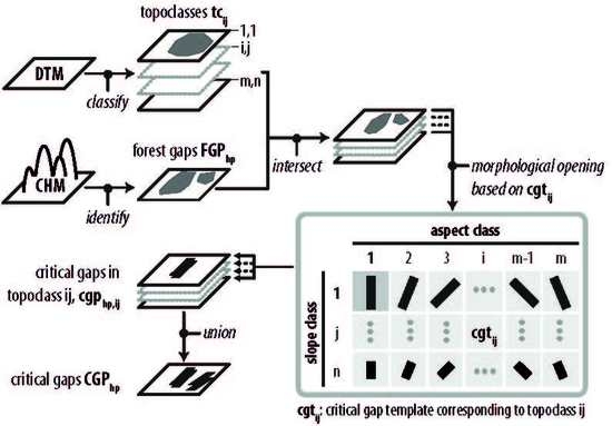
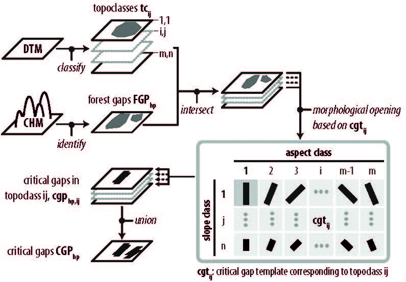
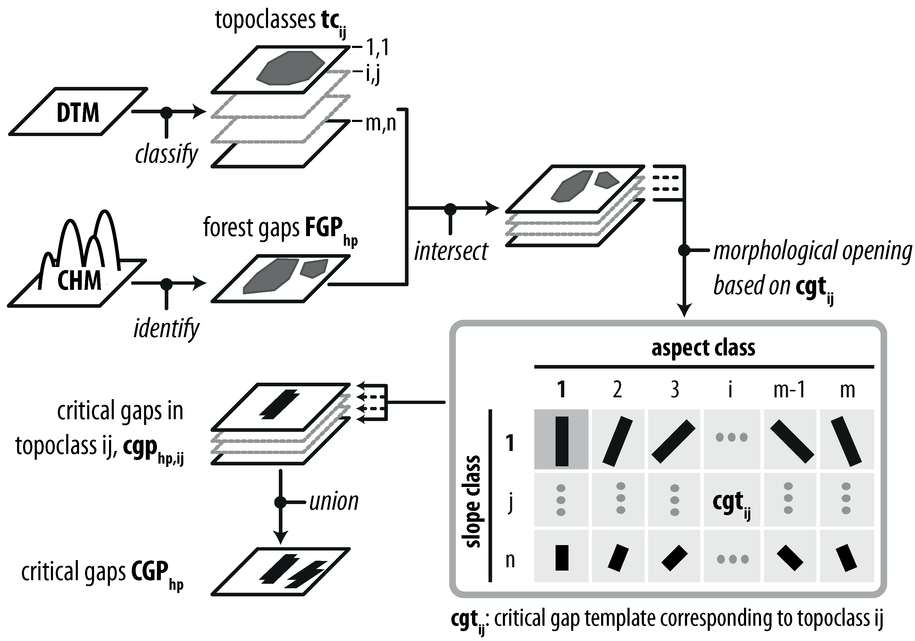
The identification of forest gaps critical to the release of avalanches compares forest-gap extents with critical-gap extents prescribed by the Swiss guidelines [5]. This comparison can be automated with a morphological opening operation () where a binary raster indicating forest gaps (=1) and forests effective against the release of avalanches (=0) is probed with a structuring element scaled to the critical-gap extent. From now on, we will use the more visual term “critical-gap template” instead of structuring element. The opening operation starts with a morphological erosion () that discards gaps which do not meet the critical-gap extent, and ends with a morphological dilation () that reconstructs the gaps at locations meeting the critical-gap extent. The slope-line direction and the length of a critical gap depend on local topography, i.e., the critical-gap template must change its extent and direction according to topography to produce plausible results. The representation of topography as a set of topographic classes with corresponding critical-gap templates makes it possible to include topography in the detection process. Figure 1 assembles these basic ideas into a workflow which we will subsequently explain.
The topography is represented as a set of topographical classes (topoclasses) . A topoclass maps locations within a specified range of hillslope steepness and slope-line directions. It results from intersecting the areas of predefined aspect classes i and slope classes j. In total, topoclasses result when computing m aspect- and n slope classes on a DTM. Forest gaps characterize the area complementary to the one sufficiently forested to be effective against the release of avalanches. The height factor h and the minimum forest coverage p define the extent of effective forests. The height factor stems from the requirement trees to be twice (i.e., ) the extreme snow height, as stated in other guidelines [7,8,9]. On the contrary to DBH ≥8 cm proposed by the Swiss guidelines [5], this tree parameter is directly measurable from a CHM. Moreover, trees meeting the expected tree height threshold values in subalpine forests are very likely to also meet the DBH-threshold. The parameters h and p control the computation of forest gaps on a CHM. Height factor h controls the selection of the tree crowns which constitute the effective forest canopy. This information is then used to calculate forest coverage. Finally, minimum forest coverage p restricts the effective forest areas to the sufficiently covered portion. The forest gaps (i.e., the complement of the effective forest area) are then intersected with each topoclass , and probed with the corresponding critical-gap template . Probing is formulated as a morphological opening as stated in Equation (7). The resulting critical gaps in all topoclasses are finally unioned to create the critical-gap map (Equation (8)). Equation (9) describes how the set notation is transferred into a binary raster where values “1” at locations r indicate critical-gap areas.
The following sub-sections explain (1) the workflows to compute topoclasses and forest gaps, (2) the approach to validate the model and (3) the model implementation.
2.1. Computation of Topographic Classes
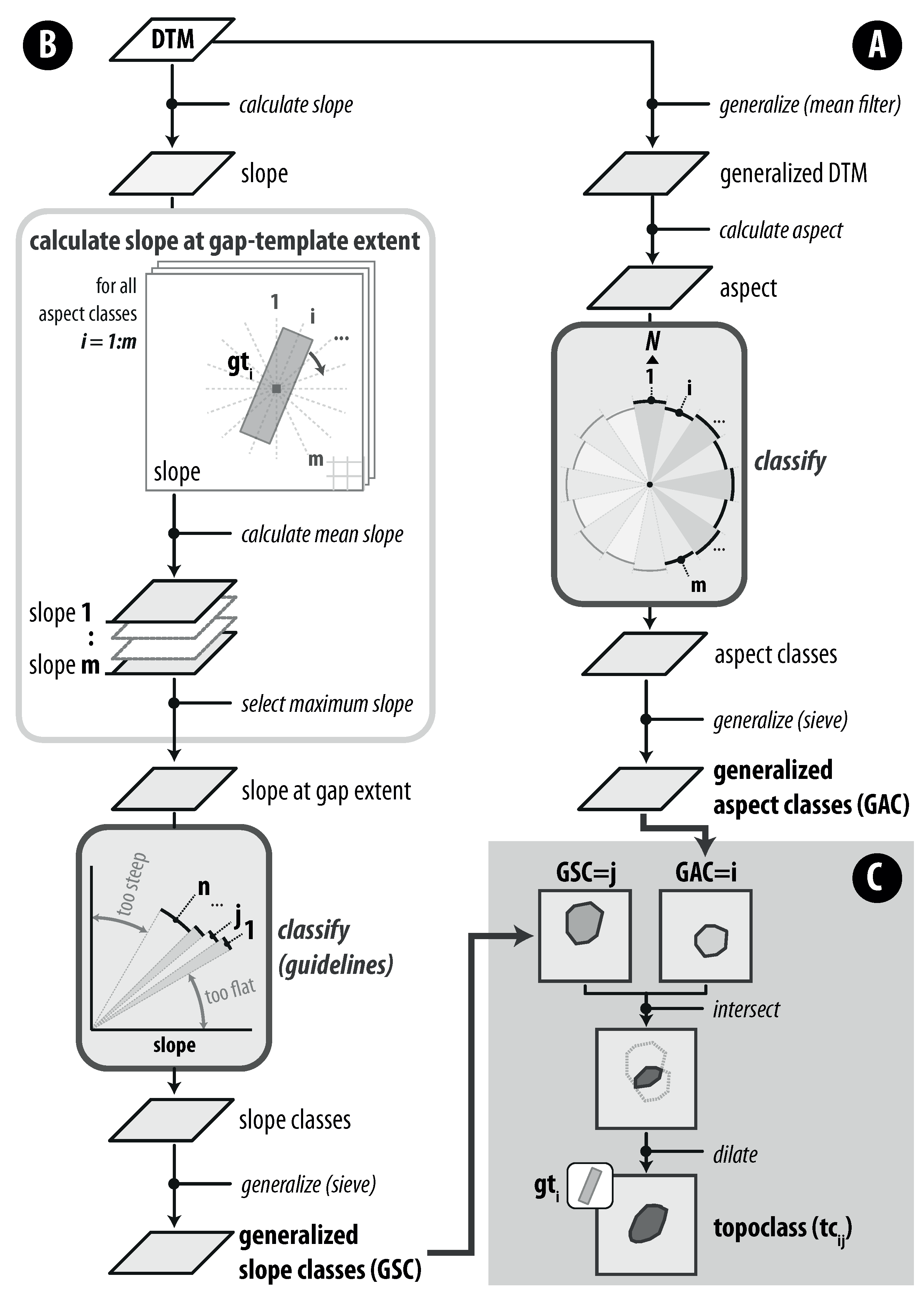
The discretization of the topography into topoclasses creates many artificial boundaries between different topoclass-patches. This may result in an underdetection of critical gaps along those boundaries. The creation of overlapping topographical classes at the appropriate scale of a critical-gap template is a means to overcome those likely limitations resulting from artificial boundaries. Figure 2C illustrates the basic principle. First, a generalized slope class j () is intersected with a generalized aspect class i (). The gap-template aligned with is then applied to the intersection to create the enlarged topoclass , which is a morphological dilation operation (Equation (10)). We will subsequently explain the detailed workflows to create and .
The generalized aspect class () raster is merely the product of classification- and generalization operations (see Figure 2B). In order to obtain contiguous aspect-class patches of sufficient extent, the aspect raster is calculated on a DTM generalized using a discoidal mean filter to obtain aspect values gradually changing in space. The raster is then classified into m aspect classes according a scheme whereby each aspect class is a merger of two ranges of degrees in opposite direction. For example, the same critical-gap template applies to North- and South-facing hillslopes. Aspect class-patches not meeting the gap template size may still exist after these operations. Therefore, those patches are finally divided-up to sufficiently large adjacent patches when applying the sieve method. The sieve method (1) identifies patches not meeting an area threshold and (2) replaces their raster values with those of the nearest raster cells belonging to valid patches.
The field evaluation of slope in a forest gap happens at the scale of a critical gap. Consequently, a slope raster must reflect the slope conditions at a similar extent. The workflow to compute generalized slope classes (, Figure 2A) adopts this conception when applying a mean filter at gap template extent () to the slope raster computed from the DTM. The maximum slope value obtained when calculating mean slope in all aspect class-directions i becomes the slope at gap extent. The values suggested by the guidelines (i.e., Table 1) serve to classify n slope classes. Finally, the sieve method is applied to divide-up patches not meeting the gap-template size.
2.2. Computation of Forest Gaps
Identification of forest gaps starts with the characterization of its complement, the forests effective against the release of avalanches. Those “effective forests” () consist of sufficiently high trees which sufficiently cover the ground. The parameters height factor h and minimum forest coverage p specify the minimum properties of effective forests , whereas multiplying h with extreme snow height gives the minimum tree height. Given set A representing the project perimeter area, the complementary set of forest gaps of is computed as follows:
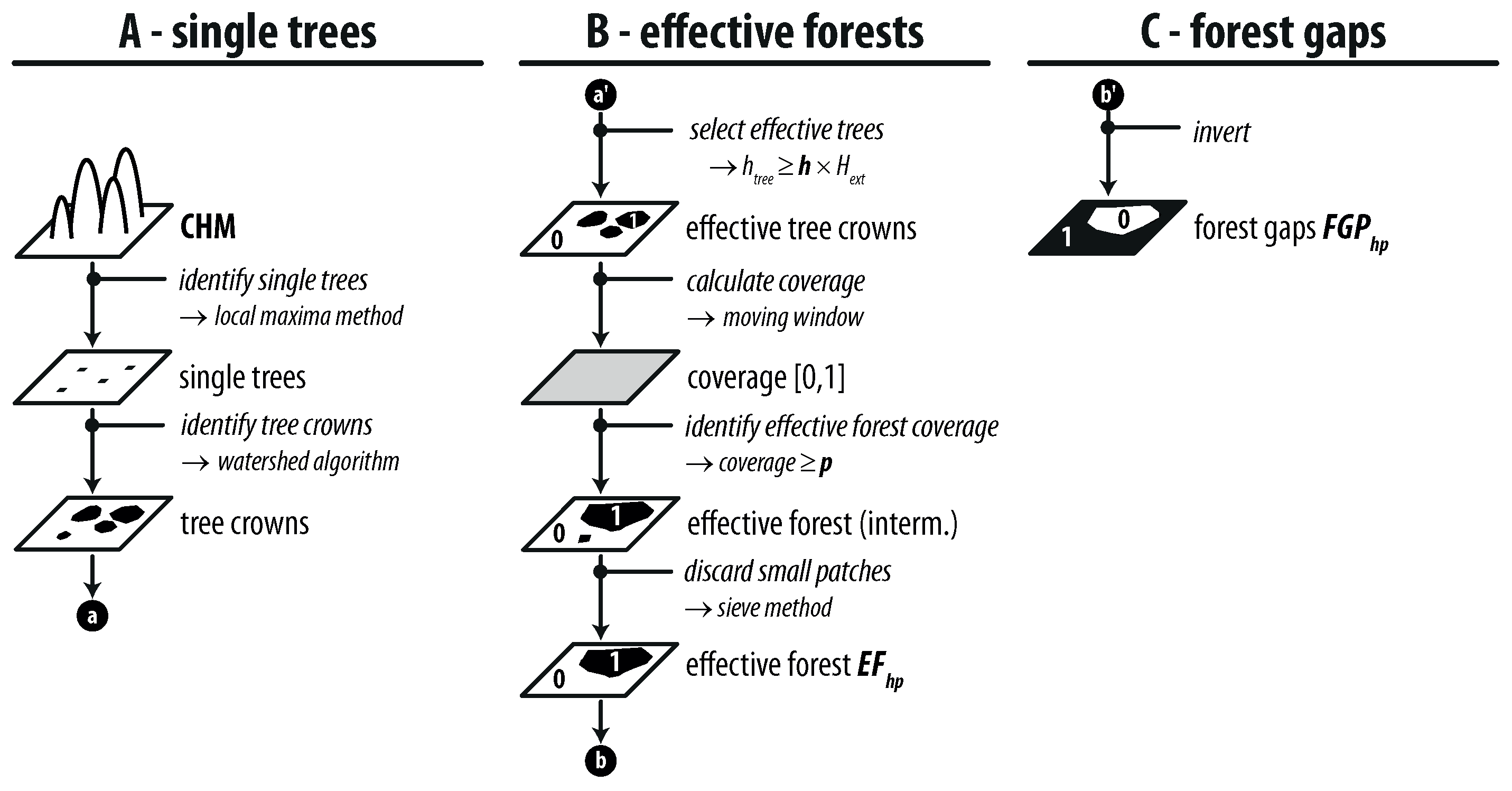
Figure 3 depicts the workflow to compute forest gaps using a canopy height model (CHM). Its principal steps are (A) the detection and characterization of single trees using the CHM, (B) the identification of effective forests using the single tree-information and (C) the identification of forest gaps as the complement of effective forests. Single trees are detected by applying a local maxima method to identify treetops and the watershed algorithm to delineate the corresponding tree crown extents on the CHM (Figure 3A). Therefore, the CHM is smoothed using a Gaussian filter (3 × 3, ) to prevent the local maxima method from overdetection, and applying a 2 m-lower height cutoff prevents the watershed algorithm from delineation of implausibly large tree crowns. The tree height [m] and the corresponding crown extent finally characterize each single tree. Effective forests are identified when selecting sufficiently high single trees, computing forest coverage for that selection and discarding effective forest patches too small to be termed “effective” (Figure 3B). Only trees equal or higher than the product of extreme snow height and height factor h are selected (Equation (12)). Here, the extreme snow height equation applied for dimensioning avalanche protection barriers (Equation (13), [13]) is adopted, which calculates [m] as a function of a region parameter [scalar] and altitude Z [m a.s.l.].
A binary raster capturing the crown extents of effective trees (=1) then serves to calculate forest coverage and to identify effective forests. Forest coverage is calculated as the share covered by effective trees within a discoidal moving window at the scale of critical-gap width. The binary effective forest raster then results from classifying forest coverage into effective forests (=1) for values ≥p and into ineffective ones for values <p. Patches not meeting a minimum extent are treated as ineffective and are discarded in the final effective forest raster by applying the sieve method. Finally, the forest gap raster results from inverting the effective forest raster (Figure 3C).
2.3. Model Validation
The TIMA-based detection of critical gaps will produce a critical-gap map. That map is interpreted as a binary classification of critical-gap presence, either being YES or NO. This enables the validation via a map accuracy assessment as proposed by Congalton and Green [47], given a set of locations where gap criticality has been assessed in the field. Here, we explain the set-up of the field survey. It aims at (1) randomly drawing sample locations supporting the explanatory power of the assessment and (2) allowing for an analytic and fast manual field assessment.
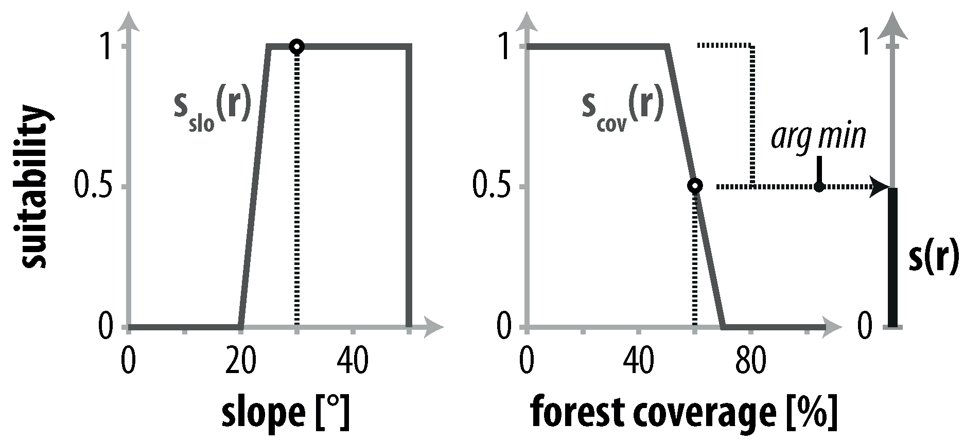
Critical gaps are assumed sparsely distributed in space because site properties are often not suited to the occurrence of critical gaps at all when hillslopes are too shallow or forests are stocked too densely. I.e., the area where critical-gap presence will be classified NO will outnumber the YES-area by far. For example, given that critical gaps make up 5% of the overall area, the chance of picking at least 5 critical-gap locations out of 50 samples is 10%, assuming a Bernoulli process. That sample dataset would support the accuracy assessment for the absence rather than for the presence of critical gaps. Instead, the principles of the Poisson sampling method [48] are adopted to produce a better balanced sample set. The method assigns potential samples an inclusion probability. That probability characterizes the sample’s suitability to support a global prediction and is scaled with the expected number n of samples to be drawn from a set N. In the context of this study, inclusion probability characterizes a location r’s suitability for critical gaps scaled with the expected number of samples n (Equation (14)). Therefore, the test area is discretized into a 25 × 25 m raster to create the set of potential sample locations N. Suitability is assessed to the same extent based on the weighting functions and that capture the suitability of local mean slope and forest coverage to encounter critical gaps. Suitability is specified by expert’s opinion on the range [0, 1] for both suitability functions (Figure 4).
The function formulation aims at obtaining a balanced sample set consisting of sample locations both with and without critical gaps. Since suitability is the product of steep slopes and sparse forest coverage, the logical AND-operation used in Fuzzy Logic [49] is adopted to compute (Equation (15)).
The field assessment is set up as a questionnaire consisting a sequence of dichotomous questions (Table 2). The assessment stops when a response to a question is negative. I.e., all responses must be positive at a sample location to become a critical gap. A differential GPS (TopCon HiPer Pro) serves to navigate to sample locations, and gap-slopes and -extents are measured using the Haglöf Vertex IV.
2.4. Model Implementation
The model was implemented using ArcGIS and MATLAB whereas the latter served to tackle processing steps for which no standard tools in ArcGIS existed. Single trees were delineated in MATLAB and topoclasses were computed in ArcGIS (ESRI, version 10.4.1), using the sieve method provided in the Geomorphometry & Gradient Metrics Toolbox [50]. The detection of critical gaps was finally implemented using the morphology operators provided in MATLAB’s Image Processing Toolbox™(The Mathworks Inc., Release 2014b).
3. Application to a Subalpine Study Area
The topography-informed morphology approach (TIMA) was tested for a subalpine study area in Klosters-Serneus (Switzerland) at the extent of 30 hectares. The forest predominantly composed of Norway spruce (Picea abies) stretches on a North-Eastern facing hillslope at elevations ranging from 1500–1700 m a.s.l.. Consequently, the specification of TIMA followed the Swiss guideline-specifications for evergreen subalpine coniferous forests. The study area was part of an airborne LiDAR acquisition in 2010 (see Table 3 for specifications). TopoSys used its own software TopPit to compute the DSM and DTM at 0.5 × 0.5 m raster resolution. The CHM resulted when subtracting the DTM from the DSM. The following sub-sections (1) explain the set-up of topography in TIMA, (2) explain the set-up of forest gaps in TIMA and investigate the sensitivity of critical-gap detection on the parameters defining effective forests, (3) investigate critical-gap map accuracy when comparing with a sample set assessed in the field, and (4) document the effect of adding linear features (i.e., forest roads and river channels) decoupling the snow layer to TIMA.
3.1. Set-Up of Topography in TIMA
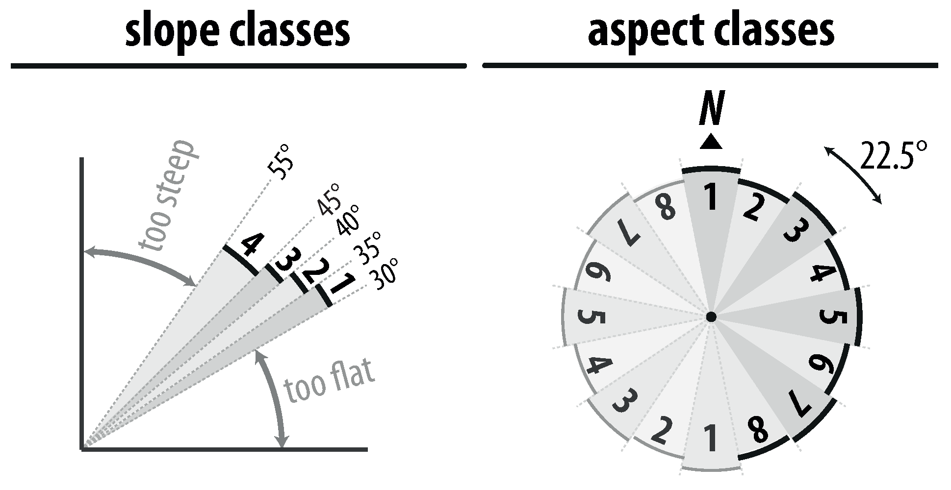
32 topoclasses captured the topography in the study area, four slope- and eight aspect classes (Figure 5). Hillslope directions were discretized using aspect classes covering 22.5°-ranges of directions to produce plausibly facing critical gaps. The aspect classes were calculated on a generalized DTM (discoidal mean filter, radius: 20 m) whereas patches not meeting an area of a representative critical gap (400 m) were modified using the sieve method explained above. The slope classification adopted the slope thresholds prescribed in the Swiss guidelines (Table 1, [5]) and restricted the steepest slope class to 55°. Slopes outside the slope class-ranges were either considered too flat or too steep for avalanche release (Figure 5). A gap template () of 10 × 30 m extent served to calculate slopes at gap extent from the slope raster that was computed on the DTM. Again, the sieve method was then applied to update patches not meeting 400 m. The resulting generalized aspect- and slope rasters (, ) were then intersected, and dilated using . The creation of the 32 critical-gap templates () corresponding to the topoclasses required the specification of gap direction, critical length and critical width. The aspect class center-values defined the direction, the critical length corresponded to the planar length of the gap length in slope line-direction (Table 1), and the gap width was set to 10 m.
3.2. Sensitivity of Critical-Gap Detection on Effective-Forest Specification
The forest gaps were first computed based on the specifications for height factor h = 2 and minimum forest coverage p = 50% as prescribed by the Swiss guidelines [5,8]. The computation followed the workflow depicted in Figure 1. This resulted in effective tree heights ranging from 6.8 to 7.8 m when parametrizing Equation (13) for Klosters-Serneus (). Effective trees were selected according to Equation (12) from the single trees delineated on the CHM. The corresponding effective tree crowns were used to estimate forest coverage at the extent of a 15 m-diameter disc (area = 180 m). The effective forest raster resulting for p = 50% was finally generalized when discarding forest compartments ≤100 m. This value corresponds to the extent of 2–3 mature trees which was assumed ineffective to prevent avalanche releases. That effective forest raster was termed the BASE raster, which was used as the starting point for the following sensitivity analysis.
The sensitivity analysis focused on how the area (1) of effective forests and (2) critical gaps changed as a result of varying tree height factor h and forest coverage p by ±20%. For example an increase of minimum forest coverage (p = 50%) by 20% resulted in p = 60%. Figure 6 shows the percental change in effective forest area related to the BASE raster (marked with a “*”). It shows that the delineation of effective forests was much more sensitive to changes in forest coverage (∼15%) than to those in the height factor (∼3%). A change in forest coverage affected the entire area whereas changes in the height factor only affected areas at the thicket stage. The latter usually forms a small portion in Swiss subalpine forests, which are managed according to long rotation periods. A maximum change of 18% resulted when both parameters were varied simultaneously.
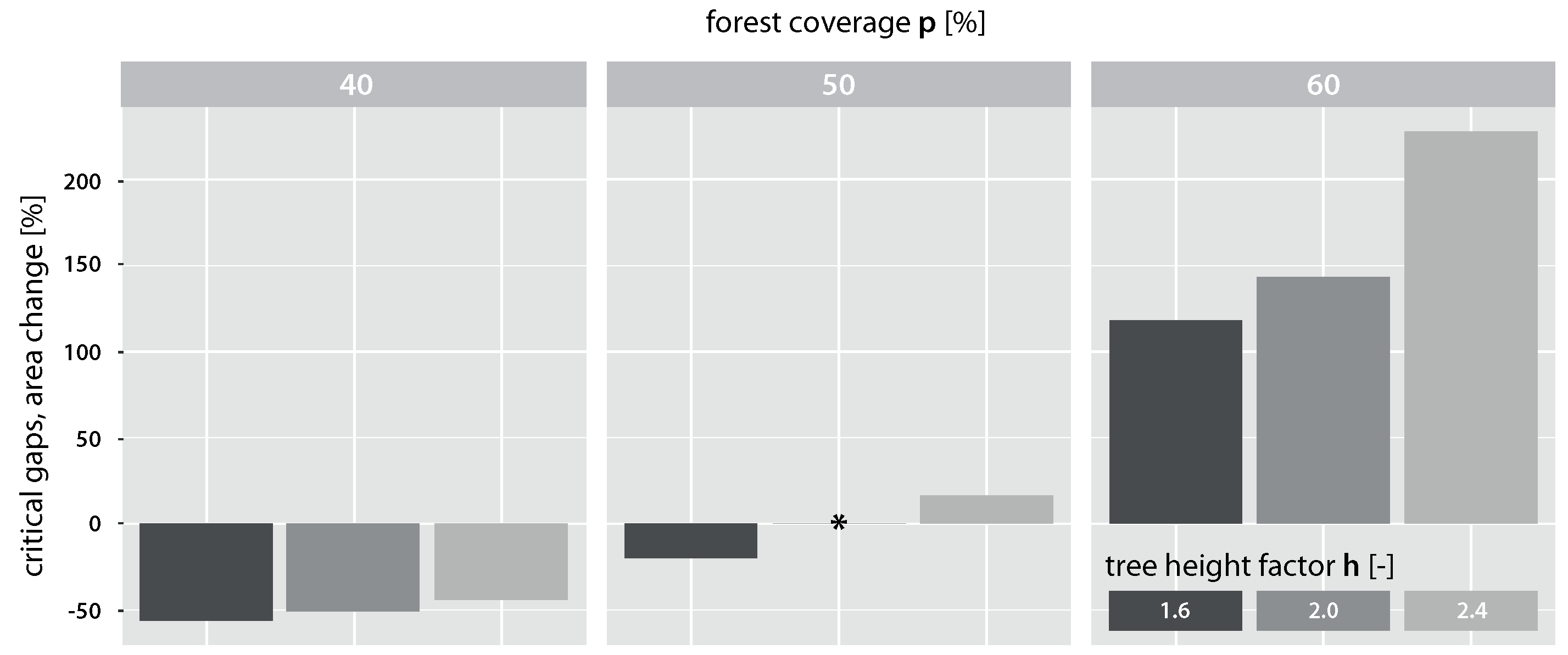
Figure 7 shows the percental change in critical-gap area related to the BASE raster (*). It indicates that the detection of critical gaps was much more sensitive to changes in forest coverage than to changes in the tree height factor. For example, the critical-gap area increased by 143% when increasing p by 20%, whereas increasing h by 20% resulted only in a 16% increment. The simultaneous variation of both parameters resulted in area changes ranging from −56% up to +228%.
The high sensitivity of critical-gap detection on the parameters specifying effective forests has led us to the conclusion that mapping of critical gaps must also communicate their sensitivity to effective forest-specification. A “gap detection rate” was identified a convenient metric to map both the location and sensitivity of critical gaps. It explains which share of alternative effective forest-specifications resulted in a critical gap on each raster cell. Detection rates close to 1 characterize gaps insensitive to the parametrization whereas detection rates close to 0 indicate the opposite. Given parameter sets H and P for the tree height factor and forest coverage used for the sensitivity analysis, the detection rate raster GAP was specified as follows:
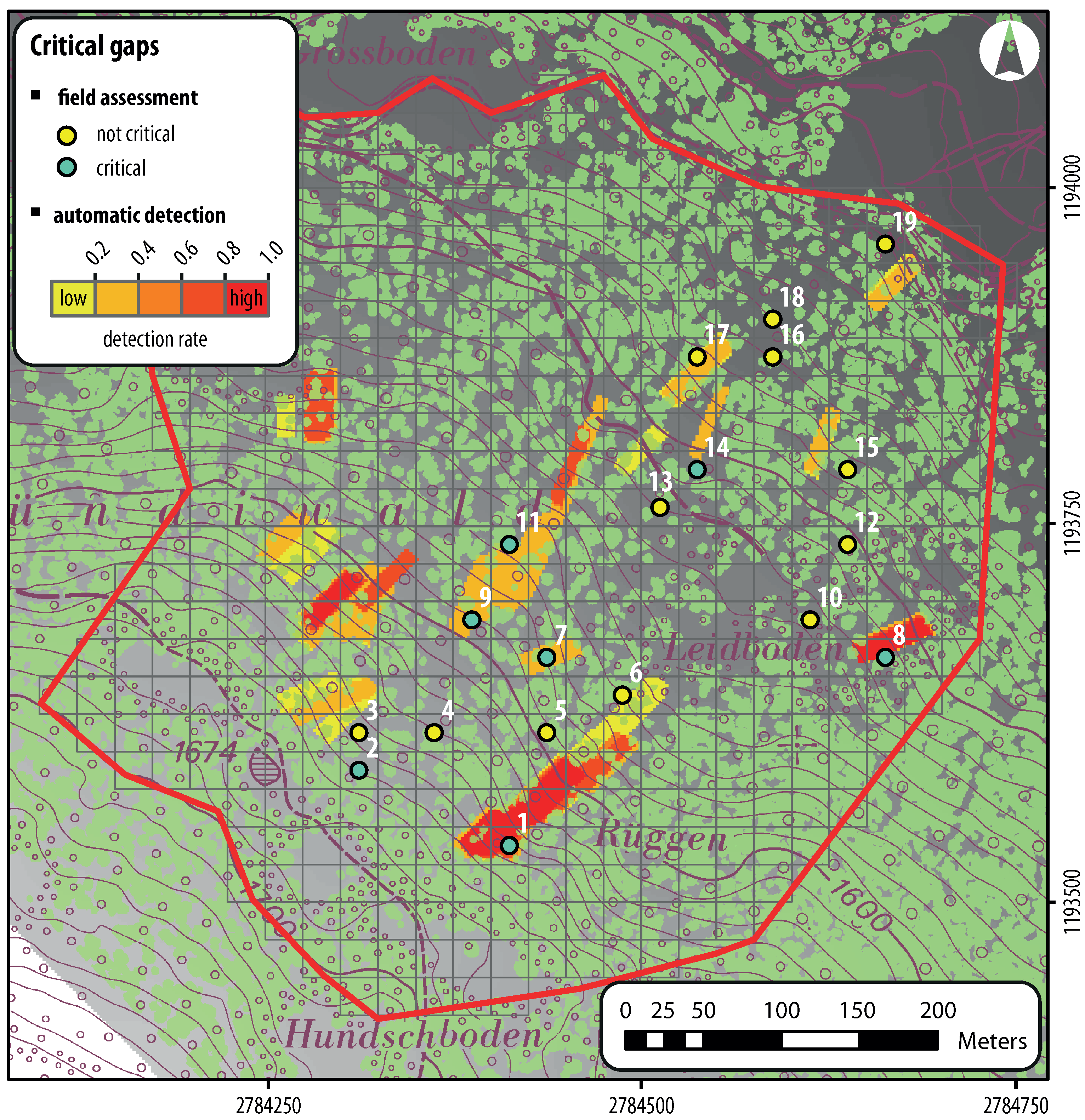
This required us to compute the binary critical-gap rasters for all -combinations where 1 indicates critical and 0 not critical in the resulting rasters. The gap detection rates were computed for the sets and . Figure 8 depicts the resulting critical-gap map which was subject to the following investigations. It displays the critical gaps overlaid with a topographic map, which allowed for a visual plausibility check.
3.3. Map Validation
The critical-gap map in Figure 8 was subject to validation using a sample set assessed in the field. The field survey was set-up according to the method explained in Section 2.3 for n = 40 sample locations. Therefore, the Poisson sampling was set-up for n = 40 locations. The application to the test area resulted in 39 samples of which a subsample of 19 in the eastern part of the study area was finally selected because of their proximity. These sample locations were visited in the field to manually assess the criticality of gaps (either being YES or NO) when applying the questionnaire (Table 2). Table A1 in the appendix shows the decision on criticality as well as the step in the questionnaire determining non-criticality for each sample.
The map in Figure 8 shows the results of the field assessment and the automatic detection (critical-gap map). Table 4 puts the comparison of the two results into an error-matrix and provides the corresponding accuracy metrics. Overall, the accuracy of detecting the presence or absence of a critical gap was 84%. The user’s accuracies, i.e., the accuracy of encountering the map prediction in the field, were 75% for the presence and 91% for the absence of critical gaps. Finally, a Kappa-value = 0.67 indicated a substantial agreement between field observation and detection according to Landis and Koch [51]. Three out of the 19 samples were misclassified, namely samples 2, 6 and 17. The reasons were manifold. The gap length and slope values in sample 2 only marginally fulfilled the criteria for a critical gap in the field. Sample 6 was not termed a critical gap in the field because of the presence of a dense forest at the thicket stage. Finally, sample 17 was not termed a critical gap because the break in the hillslope created by a wooden hillslope stabilization structure was assumed to decouple the snow layer.
3.4. Linear Features Decoupling the Snow Layer
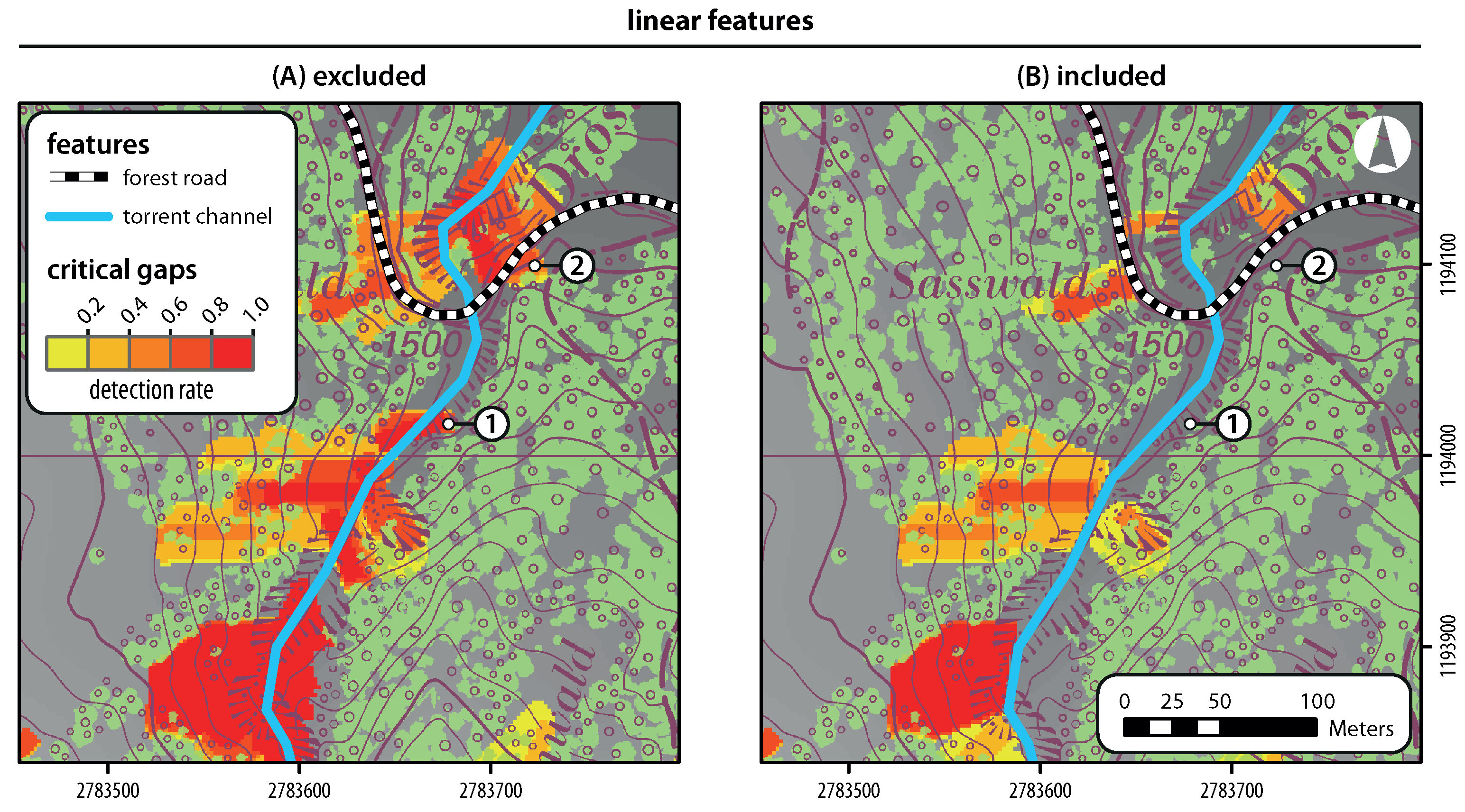
TIMA currently represented the topography at critical-gap scale, i.e., TIMA interpreted it as inclined planes at the 10 × 30 m-extent. This representation could not capture abrupt breaks on the hillslope, which can decouple the snow layer. Linear features such as torrent channels or forest roads can indicate such abrupt breaks. Earth works required when constructing forest roads result in considerable breaks on the hillslope. Moreover, a torrent channel on steep sites even indicates the conjunction of two hillslopes facing into different directions. Thus, TIMA must include those linear features to reduce overprediction resulting from generalization of topography. Features indicating abrupt breaks on the hillslope B were implemented in TIMA when added to the set of effective forests (Equation (17)). This made it impossible to detect critical gaps across these features.
An extent containing a forest road and a torrent channel was selected in the study area to test the modified model. Both, the 3.50 m wide forest road and the deep channel of the Drosbach torrent, were previously identified as abrupt breaks on the hillslope in the field, i.e., critical gaps crossing those features were implausible. The forest roads and the torrent channels were available in vector format. The cantonal forest agency of Grisons provided the forest road layer. For the sake of simplicity, the torrent channel was digitized from the topographical map in Figure 9 for the extent displayed. They were transferred into rasters to perform the computation. To perform this task, the line features were previously transferred to polygons of 3 m width. Figure 9 illustrates the resulting maps when (A) excluding and (B) including these line features. Critical gaps disappeared where the hillslopes became too short to fit a critical-gap template after adding the line features. Implausible critical gaps such as the ones at locations 1 and 2 could be erased.
4. Discussion
We have learned the following when applying the topography-informed morphology approach (TIMA) to the 30 hectare study area in Klosters-Serneus (Switzerland):
- Single trees delineated on the CHM are a convenient means to identify forests effective against the release of snow avalanches based on forest parameter thresholds. The detection of critical gaps turned out to be very sensitive to the thresholds for forest parameters that specify effective forests. For example, raising the minimum required forest coverage from 50 to 60% resulted in a 130%-increment of critical-gap area. Therefore, mapping critical gaps using detection rates appropriately communicates both the locations of critical gaps and their sensitivity to effective forest parametrization.
- The critical-gap map identifies areas with and without critical gaps at an 84% overall accuracy when compared with the results of a field assessment (n = 19). The Kappa value = 0.67 indicates substantial agreement between detection and field observation.
- TIMA can include linear features (forest roads and torrent channels) that decouple the snow layer when updating the forest gap raster with their locations. Thus, the generalized topography-characterization based on topoclasses can be improved with local topography information decisive to critical-gap detection.
These findings have important implications not only for future research but also for practitioners. Based on our experience gained from the application of TIMA to the Kloster-Serneus study area, we also identified aspects in forest- and topography characterization for an elaborate discussion. We will subsequently address these items in detail.
4.1. Implications for Practitioners and Research
A practitioner can make use of a critical-gap map colored by detection rate to identify potential critical gaps as well as their sensitivity. The latter information particularly supports the prioritization of field surveys and eventually the application of measures. However, this prioritization should also take into account other factors triggering the release of avalanches besides gap sizes and -shapes, such as hillslope aspect, surface roughness and the redistribution of snow by wind [3]. Moreover, applications to deciduous forests would require the modification of critical-gap extents and parametrization of effective forests in the context of the Swiss guidelines [5]. A potential large-scale application would require the division into sub-areas to facilitate computation. Watersheds would be suitable sub-areas because their boundaries also apply to snow processes. Moreover, a large-scale application would require automated assessment of linear features indicating abrupt breaks on the hillslope.
The main implication for research is that a topography-informed morphology approach (TIMA) has proved to plausibly detect objects (i.e., critical forest gaps) in the landscape that change their extent and orientation with local topography. The inclusion of landscape features inhibiting those objects (i.e., effective forests and line features) restricts the detection to plausible locations. In the context of forest management in potential avalanche release zones, TIMA can be adapted to the specifications of guidelines outside Switzerland [7,9,10] because all of them base their assessment on specifications for effective forests and critical-gap extents. Moreover, the method could be of use to evaluate small avalanche release areas above the treeline where critical extent matters. The minor implication for research is that the sampling scheme inspired by Poisson sampling has been proven to select suitable samples for a binary classification when the occurrence of the classes greatly differs (i.e., locations with or without critical gaps).
In general, TIMA could be a valuable tool to identify objects where topography matters. There are three aspects to consider when setting up TIMA. First, a raster is required that allows adequate representation of the template subject to probing. As morphological operations are a time-consuming task one should prefer the satisfying raster resolution to the best available one. Second, potential underdetection should be reduced via specification of sufficient large overlapping topoclasses. Eliminating topoclass-areas not meeting the template extent and morphologically dilating topoclasses at the template-extent are means to reduce potential underdection resulting from artificial boundaries created by topoclass-patches. Third, potential overdetection introduced with the generalization of topography in the previous step must be compensated with features at the sub-scale of the template that inhibit detection. Finally, the workflow for topoclass computation (Figure 2) may be adapted for other applications depending on DTM-resolution and template size.
Concrete further applications of TIMA could address other gravitational processes such as rockfall and erosion. For example, the Swiss guidelines [5] also foresee the identification of critical objects in forests protecting against rockfall. Again, one should avoid long forest gaps in slope-line direction to reduce the acceleration of rocks due to the absence of obstacles, i.e., trees. In that case, stem locations rather than crown extents matter for characterizing the forest’s effectiveness against rockfall. Finally, the Universal Soil Loss Equation (USLE, [52]) could be a starting point to identify hillslopes critical to soil conservation goals. Slope steepness and slope length are variables of that equation, which could support the determination of critical hillslope extents.
4.2. Aspects of Forest Characterization
The assignment of the parameter value for effective forest coverage has demonstrated a strong impact on the detection of critical gaps. Traditionally, practitioners have visually assessed forest coverage at the scale of forest stands, i.e., areas of homogeneous forest structure. Since critical gaps are objects at the sub-scale of stands, forest coverage assessed at the stand-scale would have lacked the necessary spatial detail. Instead, a 180 m discoidal moving window served to compute a continuous forest coverage information from CHM-derived single trees. This also facilitated capturing the gradual changes in space of subalpine forest structure. However, the aggregation via a moving window may not reflect what we encounter at a specific location. For example, a forest gap-location on the single tree map may still have a high forest coverage because of dense forest covering half of the window. Given the highly detailed CHM-based single tree characterization, one should consider identifying effective forests directly on the tree-network resulting when linking trees to their next neighbors. For example favorable tree-to-tree distances derived from stem density (in stems per hectare) requirements [4] could be a starting point for network analysis.
There is a chance that dense forests in the late thicket stage are treated as “ineffective” when many trees do not meet the tree height requirement (as we encountered at sample site 6, see Figure 8). This requirement may be sufficient for a practitioner who may skip the rule when appropriate. Providing a map indicating single trees’ sensitivity to being termed “effective” could support the interpretation of critical gaps located in forests at the thicket stage.
4.3. Aspects of Topography Characterization
The application to the test area focused on forest characterization and the comparison of detected gaps with results from field assessment. The results provide a qualitative indication of how well 32 overlapping topoclasses represented topography. The high map accuracy indicates that topoclasses plausibly mapped slope-line directions and hillslope steepness. Moreover, the accuracy metrics also indicate that critical gaps were not systematically underpredicted, which may be the result of using overlapping topoclasses. While slope classes were prescribed by the guidelines, tuning the number of aspect classes was about identifying a good trade-off between accurateness of slope-line directions and computational time. However, future research should analytically explore how well topoclasses represent real topography and how topoclass specification impacts critical-gap detection.
TIMA also accounts for features at the sub-scale of topoclasses. Besides digitally available features used in this study (i.e., forest roads and torrent channels), more features relevant to critical-gap detection could be delineated on the DTM directly. For example, methods based on steepest ascent [53] or maximum plan curvature [54] exist to identify ridgelines. The consideration of any line feature requires prior assessment of whether it results into an abrupt break on the hillslope. Here, we visually assessed the relevant linear features in the field. Future investigations should target automation of the assessment.
5. Conclusions
The article presented a topography-informed morphology approach (TIMA) for automatic identification of forest gaps critical to the release of snow avalanches using airborne LiDAR-data. TIMA uses morphological opening to probe forest gaps with a template (i.e., structuring element) representing a critical-gap extent. Since this template must adapt to the local topography to produce plausible results, space was discretized into a set of topography classes (topoclasses) and corresponding critical-gap templates. These topoclasses covered slope- and aspect-ranges to account both for critical-gap length thresholds provided by the Swiss guidelines [5] and the gap’s orientation in slope-line direction. Topoclasses were computed on a DTM (0.5 × 0.5 m) and they spatially overlapped to facilitate seamless detection of critical gaps. Forest gaps were defined as the complement of forests effective against the release of avalanches. Effective forest-areas were computed based on single trees delineated on a CHM (0.5 × 0.5 m). Therefore, thresholds for effective tree height (being the product of extreme snow height and a height factor [8]) and forest coverage were applied to the single trees to identify effective forested areas. The critical-gap map resulted from union of all critical gaps detected on the single topoclasses. Moreover, including linear features (forest road and torrent channel) decoupling the snow layer on the hillslope in TIMA enhanced map plausibility near those features.
The approach presented here is an example of automation of rules and information acquisition originally designed for manual assessment by experts. Its application to a study area in Switzerland revealed the sensitivity of critical gap detection to the parameters specifying effective forests. Contrary to the hidden ambiguity tied to an expert’s judgement on criticality, automation facilitates mapping of sensitivities as the result of model runs based on varying specifications. The promising classification accuracy of the critical-gap map indicates TIMA’s ability to capture relevant landscape features at the critical-gap scale. This encourages its use in assessing other gravitational natural hazard processes. However, future work must further investigate topoclasses’ suitability to capture the relevant topographic properties. Moreover, linear features limiting detection of critical extents such as gaps should be included whenever available to compensate for the generalization induced by topoclasses. To perform large-scale applications, future work should also address automatic delineation and assessment of those features.
Acknowledgments
We thank the Remote Sensing Laboratory at the University of Zurich and the forest agency of the Canton of Grisons for providing the geodata. We also thank Andreas Hill for valuable discussions on sampling design and Rebekka Wittwer for her help in carrying out field work.
Author Contributions
J.B. and A.G. developed the model, J.B. conducted the field work and wrote the article, M.F. supervised the forest characterization in the model and edited the manuscript prior to submission.
Conflicts of Interest
The authors declare no conflict of interest.
Appendix A

Table A1.
Characterization of the 19 field samples including the steps determining non-criticality according to Table 2.
Table A1.
Characterization of the 19 field samples including the steps determining non-criticality according to Table 2.
| ID | Step Determining Non-Criticality | Critical Gap: Field | Critical Gap: Map |
|---|---|---|---|
| 1 | none | yes | yes |
| 2 | none | yes | no |
| 3 | step 3: gap too short | no | no |
| 4 | step 2: not steep enough | no | no |
| 5 | step 1: no gap | no | no |
| 6 | step 1: no gap | no | yes |
| 7 | none, trees in gap neglectable | yes | yes |
| 8 | none | yes | yes |
| 9 | none, trees in gap neglectable | yes | yes |
| 10 | step 2: not steep enough | no | no |
| 11 | none, trees in gap neglectable | yes | yes |
| 12 | step 1: no gap | no | no |
| 13 | step 2: not steep enough | no | no |
| 14 | none, trees in gap neglectable | yes | yes |
| 15 | step 3: gap too short | no | no |
| 16 | step 2: not steep enough | no | no |
| 17 | step 3: gap too short, wooden hillslope stabilization structure | no | yes |
| 18 | step 2: not steep enough | no | no |
| 19 | step 3: gap too short | no | no |
References
- Brang, P.; Schönenberger, W.; Frehner, M.; Schwitter, R.; Thormann, J.J.; Wasser, B. Management of protection forests in the European Alps: An overview. For. Snow Landsc. Res. 2006, 80, 23–44. [Google Scholar]
- Losey, S.; Wehrli, A. Schutzwald in Der Schweiz. Vom Projekt SilvaProtect-CH Zum Harmonisierten Schutzwald; Federal Office of the Environment FOEN: Berne, Switzerland, 2013; p. 29. [Google Scholar]
- McClung, D.; Schaerer, P. The Avalanche Handbook; The Mountaineers: Seattle, WA, USA, 1993; p. 271. [Google Scholar]
- Meyer-Grass, M.; Schneebeli, M. Die Abhängigkeit der Waldlawinen von Standorts-, Bestandes-und Schneeverhältnissen. In Interpraevent 1992—Conference Proceedings. Berne, Switzerland; pp. 443–454. Available online: http://www.interpraevent.at/palm-cms/upload_files/Publikationen/Tagungsbeitraege/1992_2_443.pdf (accessed on 4 March 2018).
- Frehner, M.; Wasser, B.; Schwitter, R. Sustainability and Success Monitoring in Protection Forests—Appendix 1: Natural Hazards; Federal Office for the Environment FOEN: Berne, Switzerland, 2007; p. 26. [Google Scholar]
- Margreth, S. Die Wirkung des Waldes bei Lawinen. In Proceedings of the Forum für Wissen “Schutzwald und Naturgefahren”, Birmensdorf, Switzerland, 28–29 October 2008; pp. 21–26. Available online: https://www.waldwissen.net/wald/schutzfunktion/schnee/wsl_wald_lawinen/wsl_wald_lawinen_originalartikel.pdf (accessed on 4 March 2018).
- Courbaud, B.; Gauquelin, X. Guide des Sylvicultures de Montagne-Alpes du Nord Françaises; Office National des Forêts: Grenoble, France, 2006; p. 289. [Google Scholar]
- Margreth, S.; Burkard, A.; Burri, H. Beurteilung der Wirkung von Schutzmassnahmen gegen Naturgefahren als Grundlage für ihre Berücksichtigung in der Raumplanung; National Platform for Natural Hazards (PLANAT): Berne, Switzerland, 2008; p. 51. [Google Scholar]
- Vacik, H.; de Jel, S.; Ruprecht, H.; Gruber, G. Waldtypisierung Südtirol; Autonome Provinz Bozen-Südtirol: Bozen, Italy, 2010. [Google Scholar]
- Hotter, M.; Simon, A.; Vacik, H. Waldtypisierung Tirol; Amt der Tiroler Landesregierung: Innsbruck, Austria, 2013.
- Weir, P. Snow Avalanche Management in Forested Terrain; Number 55 in Land Management Handbook, BC Ministry of Forests: Victoria, BC, USA, 2002; p. 190.
- Feistl, T.; Bebi, P.; Dreier, L.; Hanewinkel, M.; Bartelt, P. Quantification of basal friction for technical and silvicultural glide-snow avalanche mitigation measures. Nat. Hazards Earth Syst. Sci. 2014, 14, 2921. [Google Scholar] [CrossRef]
- Margreth, S. Lawinenverbau im Anbruchgebiet; Federal Office for the Environment: Berne, Switzerland, 2007; p. 136. [Google Scholar]
- Moore, I.D.; Grayson, R.B.; Ladson, A.R. Digital Terrain Modeling—A Review of Hydrological, Geomorphological, and Biological Applications. Hydrol. Process. 1991, 5, 3–30. [Google Scholar] [CrossRef]
- Maltamo, M.; Naesset, E.; Vauhkonen, J. Forestry Applications of Airborne Laser Scanning: Concepts and Case Studies Preface; Springer: Dordrecht, The Netherlands, 2014; p. 464. [Google Scholar]
- Buhler, Y.; Kumar, S.; Veitinger, J.; Christen, M.; Stoffel, A.; Snehmani. Automated identification of potential snow avalanche release areas based on digital elevation models. Nat. Hazards Earth Syst. Sci. 2013, 13, 1321–1335. [Google Scholar] [CrossRef]
- Ghinoi, A.; Chung, C.J. STARTER: A statistical GIS-based model for the prediction of snow avalanche susceptibility using terrain features—Application to Alta Val Badia, Italian Dolomites. Geomorphology 2005, 66, 305–325. [Google Scholar] [CrossRef]
- Maggioni, M. Avalanche Release Areas and Their Influence on Uncertainty In Avalanche Hazard Mapping. Ph.D. Thesis, University of Zurich, Zurich, Switzerland, 2005. [Google Scholar]
- O’Callaghan, J.F.; Mark, D.M. The extraction of drainage networks from digital elevation data. Comput. Vis. Gr. Image Process. 1984, 28, 323–344. [Google Scholar] [CrossRef]
- Soille, P. Morphological Image Analysis Principles and Applications, 2nd ed.; Springer: Berlin, Germany, 2003; p. 391. [Google Scholar]
- Koukoulas, S.; Blackburn, G.A. Quantifying the spatial properties of forest canopy gaps using LiDAR imagery and GIS. Int. J. Remote Sens. 2004, 25, 3049–3072. [Google Scholar] [CrossRef]
- Hediger, M.; Ginzler, C.; Köchli, D. Erkennung von Waldstrukturen aus flugzeuggestützten Fernerkundungsdaten—Vergleich von Airborne Laserscanning und digitaler Photogrammetrie. In Angewandte Geoinformatik 2012: Beiträge zum 24. AGIT-Symposium Salzburg; Strobl, J., Blaschke, T., Griesebner, G., Eds.; Wichmann Verlag: Berlin, Germany, 2012; pp. 62–71. [Google Scholar]
- Flood, M. Laser altimetry: From science to commercial lidar mapping. Photogramm. Eng. Remote Sens. 2001, 67, 1209–1217. [Google Scholar]
- Khosravipour, A.; Skidmore, A.K.; Isenburg, M.; Wang, T.J.; Hussin, Y.A. Generating pit-free canopy height models from airborne lidar. Photogramm. Eng. Remote Sens. 2014, 80, 863–872. [Google Scholar] [CrossRef]
- Khosravipour, A.; Skidmore, A.K.; Isenburg, M. Generating spike-free digital surface models using lidar raw point clouds: A new approach for forestry applications. Int. J. Appl. Earth Obs. Geoinf. 2016, 52, 104–114. [Google Scholar] [CrossRef]
- Wang, Y.; Weinacker, H.; Koch, B.; Sterenczak, K. Lidar point cloud based fully automatic 3D single tree modelling in forest and evaluations of the procedure. Int. Arch. Photogramm. Remote Sens. Spatial Inform. Sci. 2008, 37, 45–51. [Google Scholar]
- Korhonen, L.; Korpela, I.; Heiskanen, J.; Maltamo, M. Airborne discrete-return LIDAR data in the estimation of vertical canopy cover, angular canopy closure and leaf area index. Remote Sens. Environ. 2011, 115, 1065–1080. [Google Scholar] [CrossRef]
- Holmgren, J.; Johansson, F.; Olofsson, K.; Olsson, H.; Glimskär, A. Estimation of crown coverage using airborne laser scanning. In Proceedings of the SilviLaser, Edinburgh, UK, 17–19 September 2008; pp. 50–57. [Google Scholar]
- Andersen, H.E.; Reutebuch, S.E.; McGaughey, R.J. A rigorous assessment of tree height measurements obtained using airborne lidar and conventional field methods. Can. J. Remote Sens. 2006, 32, 355–366. [Google Scholar] [CrossRef]
- Gaveau, D.L.A.; Hill, R.A. Quantifying canopy height underestimation by laser pulse penetration in small-footprint airborne laser scanning data. Can. J. Remote Sens. 2003, 29, 650–657. [Google Scholar] [CrossRef]
- Sačkov, I.; Hlasny, T.; Bucha, T.; Juriš, M. Integration of tree allometry rules to treetops detection and tree crowns delineation using airborne lidar data. iFor. Biogeosci. For. 2017, 10, 459–467. [Google Scholar] [CrossRef]
- Lamprecht, S.; Stoffels, J.; Dotzler, S.; Haß, E.; Udelhoven, T. aTrunk—An ALS-based trunk detection algorithm. Remote Sens. 2015, 7, 9975–9997. [Google Scholar] [CrossRef]
- Hyyppa, J.; Kelle, O.; Lehikoinen, M.; Inkinen, M. A segmentation-based method to retrieve stem volume estimates from 3-D tree height models produced by laser scanners. IEEE Trans. Geosci. Remote Sens. 2001, 39, 969–975. [Google Scholar] [CrossRef]
- Persson, A.; Holmgren, J.; Soderman, U. Detecting and measuring individual trees using an airborne laser scanner. Photogramm. Eng. Remote Sens. 2002, 68, 925–932. [Google Scholar]
- Popescu, S.C.; Wynne, R.H.; Nelson, R.F. Estimating plot-level tree heights with lidar: Local filtering with a canopy-height based variable window size. Comput. Electron. Agric. 2002, 37, 71–95. [Google Scholar] [CrossRef]
- Koch, B.; Heyder, U.; Weinacker, H. Detection of individual tree crowns in airborne lidar data. Photogramm. Eng. Remote Sens. 2006, 72, 357–363. [Google Scholar] [CrossRef]
- Kaartinen, H.; Hyyppa, J.; Yu, X.W.; Vastaranta, M.; Hyyppa, H.; Kukko, A.; Holopainen, M.; Heipke, C.; Hirschmugl, M.; Morsdorf, F.; et al. An International Comparison of Individual Tree Detection and Extraction Using Airborne Laser Scanning. Remote Sens. 2012, 4, 950–974. [Google Scholar] [CrossRef] [Green Version]
- Vauhkonen, J.; Ene, L.; Gupta, S.; Heinzel, J.; Holmgren, J.; Pitkanen, J.; Solberg, S.; Wang, Y.S.; Weinacker, H.; Hauglin, K.M.; et al. Comparative testing of single-tree detection algorithms under different types of forest. Forestry 2012, 85, 27–40. [Google Scholar] [CrossRef]
- Vincent, L.; Soille, P. Watersheds in Digital Spaces—An Efficient Algorithm Based on Immersion Simulations. IEEE Trans. Pattern Anal. Mach. Intell. 1991, 13, 583–598. [Google Scholar] [CrossRef]
- Duncanson, L.I.; Cook, B.D.; Hurtt, G.C.; Dubayah, R.O. An efficient, multi-layered crown delineation algorithm for mapping individual tree structure across multiple ecosystems. Remote Sens. Environ. 2014, 154, 378–386. [Google Scholar] [CrossRef]
- Schardt, M.; Ziegler, M.; Wimmer, A.; Wack, R.; Hyyppa, J. Assessment of forest parameters by means of laser scanning. Int. Arch. Photogramm. Remote Sens. Spatial Inform. Sci. 2002, 34, 302–309. [Google Scholar]
- Dougherty, E.R.; Lotufo, R.A. Hands-on Morphological Image Processing; SPIE Press: Bellingham, WA, USA, 2003; p. 272. [Google Scholar]
- Soille, P.; Gratin, C. An efficient algorithm for drainage network extraction on DEMs. J. Vis. Commun. Image Represent. 1994, 5, 181–189. [Google Scholar]
- Li, Y.; Zhu, L.; Tachibana, K.; Shimamura, H. Morphological operation based dense houses extraction from DSM. Int. Arch. Photogramm. Remote Sens. Spatial Inform. Sci. 2014, 40, 183–189. [Google Scholar] [CrossRef]
- Andersen, H.E.; Reutebuch, S.E.; Schreuder, G.F. Automated individual tree measurement through morphological analysis of a LIDAR-based canopy surface model. In Proceedings of the 1st International Precision Forestry Symposium, Seattle, WA, USA, 17–20 June 2001; pp. 11–21. [Google Scholar]
- Zhang, K.Q. Identification of gaps in mangrove forests with airborne LIDAR. Remote Sens. Environ. 2008, 112, 2309–2325. [Google Scholar] [CrossRef]
- Congalton, R.G.; Green, K. Assessing the Accuracy of Remotely Sensed Data Principles And Practices, 2nd ed.; CRC Press: Boca Raton, FL, USA, 2009; p. 183. [Google Scholar]
- Särndal, C.E.; Swensson, B.; Wretman, J. Model Assisted Survey Sampling; Springer: New York, NY, USA, 2003; p. 694. [Google Scholar]
- Zadeh, L.A. Fuzzy Sets. Inform. Control 1965, 8, 338–353. [Google Scholar] [CrossRef]
- Evans, J.S.; Oakleaf, J.; Cushman, S.; Theobald, D. An ArcGIS Toolbox for Surface Gradient and Geomorphometric Modeling, version 2.0-0; 2014. Available online: http://evansmurphy.wixsite.com/evansspatial/arcgis-gradient-metrics-toolbox (accessed on 4 March 2018).
- Landis, J.R.; Koch, G.G. The measurement of observer agreement for categorical data. Biometrics 1977, 33, 159–174. [Google Scholar] [CrossRef] [PubMed]
- Wischmeier, W.H.; Smith, D.D. A universal soil-loss equation to guide conservation farm planning. Trans. 7th int. Congr. Soil Sci. 1960, 1, 418–425. [Google Scholar]
- Koka, S.; Anada, K.; Nomaki, K.; Sugita, K.; Tsuchida, K.; Yaku, T. Ridge Detection with the Steepest Ascent Method. Procedia Comput. Sci. 2011, 4, 216–221. [Google Scholar] [CrossRef]
- Rana, S. Use of Plan Curvature Variations for the Identification of Ridges and Channels on DEM. In Progress in Spatial Data Handling: 12th International Symposium on Spatial Data Handling; Riedl, A., Kainz, W., Elmes, G.A., Eds.; Springer: Berlin/Heidelberg, Germany, 2006; pp. 789–804. [Google Scholar]
Figure 1.
Workflow for the automatic detection of critical forest gaps () based on a series of morphological opening operations applied to forest gaps () for various topoclasses () and their corresponding critical-gap templates (). Topoclasses are computed from the digital terrain model (DTM) and forest gaps from the canopy height model (CHM).

Figure 2.
Workflow for the computation of topoclasses () based on generalized slope- and aspect classes (, ). Part (A) depicts the steps to calculate , part (B) the ones to calculate . Part (C) explains the computation of overlapping topoclasses to overcome likely limitations resulting from artificial boundaries. Therefore, the intersections of and are morphologically dilated with the gap-template () corresponding to aspect class i.

Figure 3.
Workflow for the identification of forest gaps (). It is based on (A) the delineation and characterization of trees based on a CHM, (B) the identification of effective forests subject to height factor h and minimum forest coverage p, and (C) the inversion of to obtain forest gaps .
Figure 3.
Workflow for the identification of forest gaps (). It is based on (A) the delineation and characterization of trees based on a CHM, (B) the identification of effective forests subject to height factor h and minimum forest coverage p, and (C) the inversion of to obtain forest gaps .

Figure 4.
Suitability functions for slope and forest coverage . The minimum of the two indicates overall suitability , as indicated for the example location characterized by 30°slope steepness and 60% forest coverage.
Figure 4.
Suitability functions for slope and forest coverage . The minimum of the two indicates overall suitability , as indicated for the example location characterized by 30°slope steepness and 60% forest coverage.

Figure 5.
Classification schemes for the four slope classes and eight aspect classes constituting the 32 topoclasses subject to investigation. The slope classification corresponds to the values in Table 1.
Figure 5.
Classification schemes for the four slope classes and eight aspect classes constituting the 32 topoclasses subject to investigation. The slope classification corresponds to the values in Table 1.

Figure 6.
Sensitivity of the delineated area of effective forest on the parameters forest coverage and tree height factor. Area change is expressed as the percent change in relation to the BASE parametrization of effective forests, h = 2 and p = 50% (*).
Figure 6.
Sensitivity of the delineated area of effective forest on the parameters forest coverage and tree height factor. Area change is expressed as the percent change in relation to the BASE parametrization of effective forests, h = 2 and p = 50% (*).

Figure 7.
Sensitivity of the delineated area of effective forest on the parameters forest coverage and tree height factor. Area change is expressed as the percent change in relation to the BASE parametrization of effective forests, h = 2 and p = 50% (*).
Figure 7.
Sensitivity of the delineated area of effective forest on the parameters forest coverage and tree height factor. Area change is expressed as the percent change in relation to the BASE parametrization of effective forests, h = 2 and p = 50% (*).

Figure 8.
Results of the critical-gap classification based on the automatic detection and the results of the field assessment. Topographic map: Uebersichtsplan (UP), Canton of Grisons, 17 January 2017.
Figure 8.
Results of the critical-gap classification based on the automatic detection and the results of the field assessment. Topographic map: Uebersichtsplan (UP), Canton of Grisons, 17 January 2017.

Figure 9.
Comparison of detected critical gaps when (A) excluding and (B) including linear features that decouple hillslopes. The channel was digitized from the topographic map: Uebersichtsplan (UP), Canton of Grisons, 17 January 2017.
Figure 9.
Comparison of detected critical gaps when (A) excluding and (B) including linear features that decouple hillslopes. The channel was digitized from the topographic map: Uebersichtsplan (UP), Canton of Grisons, 17 January 2017.

Table 1.
Critical-gap lengths for avalanche release proposed by the Swiss guidelines (applies to all forest types).
Table 1.
Critical-gap lengths for avalanche release proposed by the Swiss guidelines (applies to all forest types).
| Steepness [°] | Critical-Gap Length in Slope-Line Direction [m] |
|---|---|
| ≥30 | 60 |
| ≥35 | 50 |
| ≥40 | 40 |
| ≥45 | 30 |
Table 2.
Questionnaire used for the field assessment.
| Step | Question | Action |
|---|---|---|
| 1 | Is there is a gap close to the center of the 25 × 25 m cell? | Visual inspection |
| 2 | Is the local slope equal or steeper than 30? | Measure the slope in slope-line direction within a distance of 10 m around the center |
| 3 | Is the gap long and steep enough to be classified “critical” according to the guidelines (Table 1)? | Measure the slant distance and the slope of the gap |
| 4 | Is the gap wide enough (i.e., ≥10 m)? | Measure gap width |
| 5 | Is the presence of trees in the gap neglectable? | Visual inspection whether trees are grouped |
Table 3.
Specification of the airborne LiDAR-data acquisition.
| Attribute | Unit | Value |
|---|---|---|
| Instrument | Riegl LMS Q 560 | |
| Beam deflection | Rotating mirror | |
| Time of acquisition | 11–15 September 2010 | |
| Pulse Repetition Frequency | kHz | 70 |
| Flight altitude | m | 700 |
| Max. scan angle | ° | ±15 |
| Wavelength | nm | 1550 |
| Beam divergence | mrad | ≤0.5 |
| Avg. echo density | m | 27.4 |
Table 4.
Error matrix and accuracy metrics for the comparison of critical gaps manually assessed in the field (references) with automatically detected ones (classification).
Table 4.
Error matrix and accuracy metrics for the comparison of critical gaps manually assessed in the field (references) with automatically detected ones (classification).
| Classification | References | Producer’s Accuracy[%] | User’s Accuracy[%] | ||
|---|---|---|---|---|---|
| Yes | No | Total | |||
| Yes | 6 | 2 | 8 | 86% | 75% |
| No | 1 | 10 | 11 | 83% | 91% |
| Total | 7 | 12 | 19 | Overall accuracy: 84%; Cohen’s Kappa : 0.67 | |
© 2018 by the authors. Licensee MDPI, Basel, Switzerland. This article is an open access article distributed under the terms and conditions of the Creative Commons Attribution (CC BY) license (http://creativecommons.org/licenses/by/4.0/).
Share and Cite
MDPI and ACS Style
Breschan, J.R.; Gabriel, A.; Frehner, M. A Topography-Informed Morphology Approach for Automatic Identification of Forest Gaps Critical to the Release of Avalanches. Remote Sens. 2018, 10, 433. https://doi.org/10.3390/rs10030433
AMA Style
Breschan JR, Gabriel A, Frehner M. A Topography-Informed Morphology Approach for Automatic Identification of Forest Gaps Critical to the Release of Avalanches. Remote Sensing. 2018; 10(3):433. https://doi.org/10.3390/rs10030433
Chicago/Turabian StyleBreschan, Jochen Ruben, Andreas Gabriel, and Monika Frehner. 2018. "A Topography-Informed Morphology Approach for Automatic Identification of Forest Gaps Critical to the Release of Avalanches" Remote Sensing 10, no. 3: 433. https://doi.org/10.3390/rs10030433
Note that from the first issue of 2016, this journal uses article numbers instead of page numbers. See further details here.