Landsat Super-Resolution Enhancement Using Convolution Neural Networks and Sentinel-2 for Training

Abstract

Landsat is a fundamental data source for understanding historical change and its effect on environmental processes. In this research we test shallow and deep convolution neural networks (CNNs) for Landsat image super-resolution enhancement, trained using Sentinel-2, in three study sites representing boreal forest, tundra, and cropland/woodland environments. The analysis sought to assess baseline performance and determine the capacity for spatial and temporal extension of the trained CNNs. This is not a data fusion approach and a high-resolution image is only needed to train the CNN. Results show improvement with the deeper network generally achieving better results. For spatial and temporal extension, the deep CNN performed the same or better than the shallow CNN, but at greater computational cost. Results for temporal extension were influenced by change potentiality reducing the performance difference between the shallow and deep CNN. Visual examination revealed sharper images regarding land cover boundaries, linear features, and within-cover textures. The results suggest that spatial enhancement of the Landsat archive is feasible, with optimal performance where CNNs can be trained and applied within the same spatial domain. Future research will assess the enhancement on time series and associated land cover applications.

1. Introduction

High spatial and temporal resolution earth observation (EO) images are desirable for many remote sensing applications, providing a finer depiction of spatial boundaries or timing of environmental change. Landsat provides the longest record of moderate spatial resolution (30 m) data of the earth from 1984 to present. It is currently a fundamental data source for understanding historical change and its relation to carbon dynamics, hydrology, climate, air quality, biodiversity, wildlife demography, etc. Landsat temporal coverage is sparse due to the 16-day repeat visit and cloud contamination. Several studies have addressed this through time series modeling approaches [1,2,3]. Temporal enhancement is a key requirement, but spatial enhancement is another aspect of Landsat that could be improved for time series applications. Enhancement of spatial resolution has been carried out mostly based on data fusion methods [4,5,6,7]. Studies have also shown that data fusion can lead to improvements in quantitative remote sensing applications such as land cover [4,8,9]. Although effective, data fusion techniques are limited by the requirement for coinstantaneous high-resolution observations. For more recent sensors such as Landsat-8 and Sentinel-2 this requirement is met with the panchromatic band and provides the greatest potential for spatial enhancement. However, for a consistent Landsat time series from 1985 to present, a method that will provide the same level of enhancement across sensors is needed. For Landsat-5, a suitable high-resolution source is generally inadequate in space or time to facilitate generation of an extensive spatially enhanced Landsat archive.

Numerous spatial resolution enhancement methods have been developed. However, recently, deep learning convolution neural networks (CNNs) have been shown to outperform these, with large improvements over bicubic and smaller gains over more advanced anchored neighborhood regression approaches [10]. CNNs are a special form of neural network. The basic neural network is made up of a collection of connected neurons with learnable weights and biases that are optimized through error backpropagation [11]. The input is a vector, whereas the input to a convolution neural network is an array or image. For each convolution layer, a set of weights are learned for a filter of size m × n × c that is convolved over the image, where m and n are vertical and horizontal dimensions and c is the input features to the convolution layer. Essentially, a convolution neural network can learn the optimal set of filters to apply to an image for a specific image recognition task. Thus, one strategy has been to use CNNs as feature extractors in remote sensing classification applications [12].

There has been significant development of CNNs for super-resolution enhancement with non-remote sensing image benchmark databases such as CIFAR-100 [13] or ImageNet [14]. Dong et al. [10] developed the Super-Resolution Convolutional Neural Network (SRCNN), which used small 2 and 4 layer CNNs to show that the learned model performed better than other state of the art methods. Kim et al. [15,16] developed two deep convolutional networks for super-resolution enhancement. The first was the Deeply-Recursive Convolutional Network for Image Super Resolution (DRCN), which used recursive or shared weights to reduce model parameters in a deep 20-layer network. The second was also a deep 20-layer network (Very Deep Super Resolution, VDSR), but introduced the concept of the residual learning objective. In this approach, instead of learning the fine resolution image, the differences between the fine and coarse resolution images are learned. This led to significant performance gains over SRCNN. The mean squared error loss is widely used for CNN super-resolution training. An interesting alternative was tested by Svoboda et al. [17] who used a gradient based learning objective, where the mean squared error between spatial image gradients computed using the Sobel operator was sought to be minimized. Performance by standard measures, however, were not improved. Mao et al. [18] developed a deep encoder-decoder CNN with skip connections between associated encode and decode layers. It achieved improved accuracy relative to SRCNN for both 20 and 30-layer versions. An ensemble based approach was tested in Wang et al. [19] and was found to provide an improvement in accuracy. Other methods have focused on maintaining or improving accuracy while reducing the total model parameters. The Efficient Sub-Pixel Convolutional Neural Network (ESPCN) reduces computational and memory complexity, by increasing the resolution from low to high only at the end of the network [20]. The DRCN approach [15] was extended to include residual and dense connections by Tia et al. [21]. This provided a deep network with recursive layers reducing the model parameters and achieving the best results for the assessment undertaken.

Residual connections in CNNs were introduced by He et al. [22] for image object recognition. Residual connections force the next layer in the network to learn something different from the previous layers and have been shown to alleviate the problem of deep learning models not improving performance with depth. In addition to going deep, Zagoruyko and Komodakis [23] showed that going wide can increase network performance for image recognition. More recently, Xie et al. [24] developed wide residual bocks, which adds another dimension referred to as cardinality in addition to network depth and width. The rate of new developments in network architectures is rapid with incremental improvements in accuracy or reductions in model complexity and memory requirements.

For spatial enhancement of remote sensing imagery, much less research has been carried out regarding the potential of CNNs. Only recently have results been presented by Collins et al. [25] who applied networks similar to Dong et al. [10] for enhancement of the Advanced Wide Field Sensor (AWiFS) using the Linear Imaging Self Scanner (LISS-III). Their study provides a good benchmark for CNN performance because the two sensors have the same spectral bands and are temporally coincident. Results showed similar performance to other CNN based super-resolution studies for the scaling ratio of 2.3 (56 m/24 m spatial resolution).

Advances in deep learning CNNs and the global availability of Sentinel-2 data provide a potential option to generate an extensive spatially enhanced historical Landsat archive. Conceivably, a relatively cloud free Landsat and Sentinel-2 image will be obtained within a suitable temporal window for most locations across the globe. Thus, a consistent image pair suitable for training a Landsat super-resolution transform may be obtained and could be locally optimized for this purpose following the approach applied in Latifovic et al. [26]. However, for large area implementation, CNN performance across a variety of landscapes needs to be evaluated in addition to temporal and spatial extension capacity. Therefore, specific objectives of this research were to:

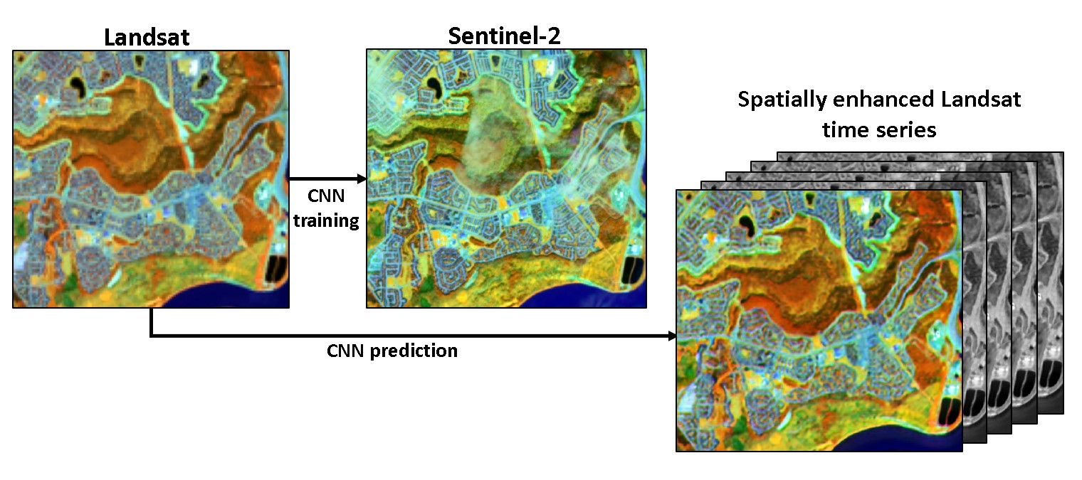
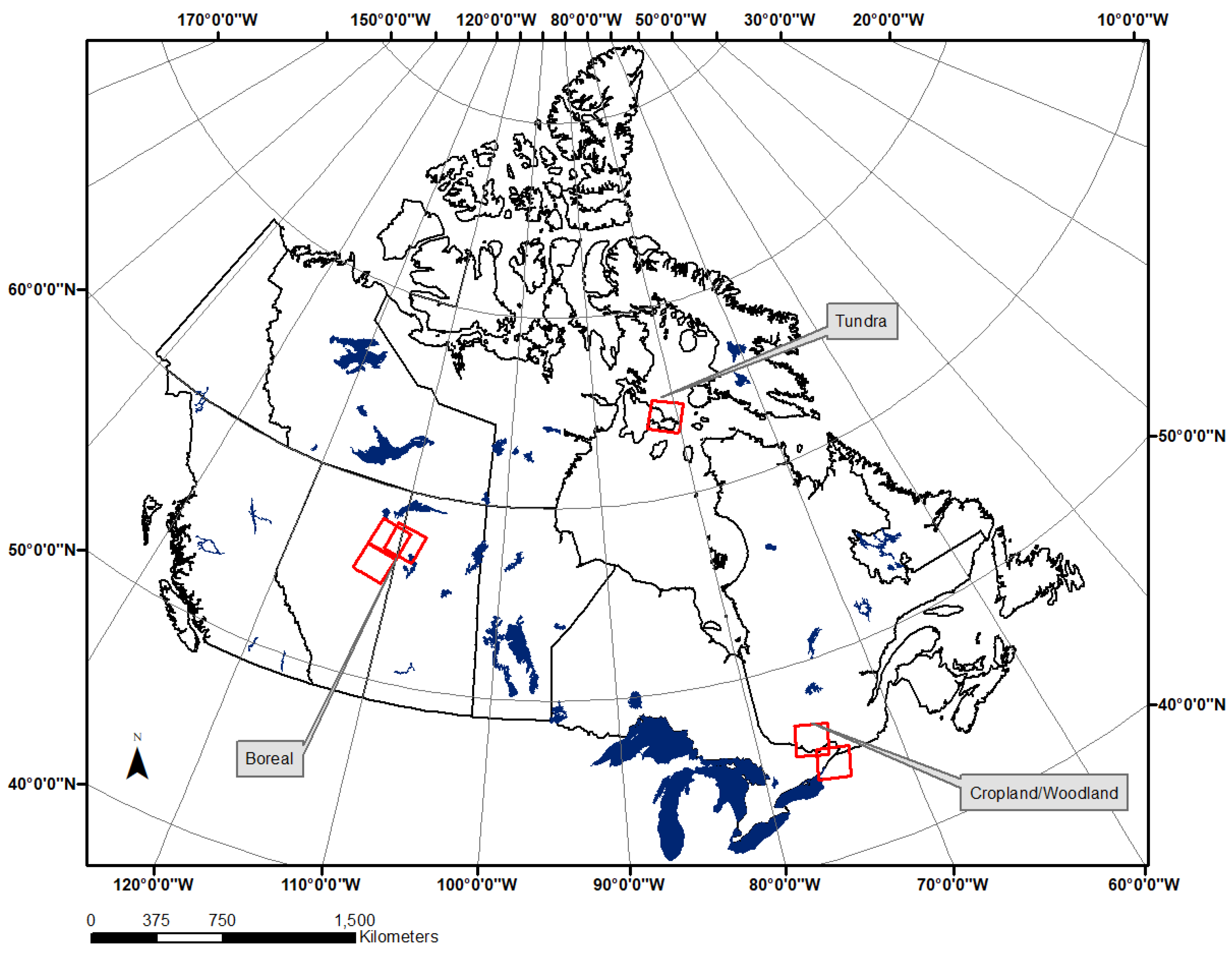
• Assesses the effectiveness of a shallow and deep CNN for super-resolution enhancement of Landsat trained from Sentinel-2 data for characteristic landscape environments in Canada including boreal forest, tundra, and cropland/woodland landscapes.
• Evaluate the potential for spatial extension over short distances of less than 100 km and temporal extension of a trained CNN model.

2. Materials and Methods

2.1. Landsat and Sentinel-2 Datasets

For model development, Landsat-5, 8 and Sentinel-2 pairs for three study areas in Canada were acquired. The study areas are shown in Figure 1 and included boreal forest, tundra, and cropland/woodland ecosystems. These represent a range of ecosystem conditions found in Canada. If the performance is acceptable across these three, it is likely that similar performance can be obtained across the range of ecosystems found in Canada in non-complex terrain.

The date ranges of the training image pairs are given in

Table 1. Landsat and Sentinel-2 images used for training and testing.

Region	Sentinel-2		Landsat-8		Landsat-5
	Tile Reference	Date	Tile Reference	Date	Tile Reference	Date
Boreal	T12VWH 8	7/19/2016	40_20	7/17/2016	42_20	7/31/1984
	T12VVH 8	8/30/2016	42_20	7/15/2016	42_20	8/28/1997
	T12VVJ 5	7/9/2017	42_21	8/30/2015	42_20	7/20/2011
Tundra	T17VML 5,8	8/14/2016	26_15	8/16/2016	26_15	8/1/1987
	T17WMM 5,8	8/13/2016			26_15	8/4/1994
	T17WMM 5,8	8/13/2016			26_15	7/15/2010
Cropland/Woodland	T18TVR 5,8	7/20/2016	15_29	8/19/2016	16_28	8/11/1987
	T18TWR 5,8	7/20/2016	16_28	8/26/2016	16_28	7/3/2002
			16_28	8/26/2016	16_28	8/2/2007

Tile reference for Landsat is Path_Row format. Superscripts for Sentinel-2 tiles denote which Landsat sensor was used, 8 is Landsat-8 and 5 is Landsat 5.

. Landsat level 2 surface reflectance collection 1 was acquired from the USGS. Sentinel-2 level-1C data was also acquired from the USGS and converted to surface reflectance using the sen2cor algorithm version 2.3.1 (European Space Agency) [27]. Landsat-8 and Sentinel-2 have spatial misalignment that varies regionally depending on ground control point quality [28]. It has been improved for collection 1 data in global priority areas. More recent analysis shows that collection 1 Landsat-8 data within Canada (approximately lower than 70 degrees latitude) has a horizontal root mean square error (RMSE) of less than 14 m [29]. The geolocation quality of all input images was checked by collecting control points and computing the RMSE. For all scenes the RMSE was less than 10 m. The largest error was in the northern tundra study site and areas within or close to cloud cover. This error was considered reasonable given the expected operational geolocation accuracy and effective resolution of the spatial enhancement being tested. Landsat data were resampled to 10 m resolution using the nearest neighbor approach. This was selected to maintain spectral quality, allow the CNN to determine the optimal spatial weighting, and speed local resampling for application to large images. All Landsat and Sentinel-2 scenes were mosaiced and stacked together for analysis in each study site.

As identified in Latifovic et al. [30] and specified in the USGS documentation [31], atmosphere correction can be problematic in the north above 64 degrees latitude. Our northern study area was at approximately 64 degrees. However, this was not considered to be a problem as errors due to atmosphere correction would be similar between the datasets and would not affect the relative comparison of the methods.

2.2. Sampling and Assessment

For each study site a mask was manually developed for sampling to avoid clouds, shadows, and land cover changes between the image mosaic pairs. However, in cropland environments the 26-day difference between the Landsat-8 and Sentinel-2 images made it impractical to manually define areas suitable for training. Thus, for this study site an initial mask was developed, but refined by calculating the change vector between images [32] and selecting a conservative threshold to avoid including cropland change in the training. The local variance within sample windows of 33 by 33 pixels was computed and used define three levels of low, moderate, and high spatial complexity. These represented homogenous areas at the low level to areas containing significant structure related to roads, shorelines, or other boundaries at the high level. This was used in a stratified systematic sampling scheme to ensure a range of spatial variability was selected. For each stratum, every sixth pixel was selected not contaminated by clouds or land cover change. To assess performance, we compute the mean error, mean absolute error (MAE), error standard deviation, and mean and standard deviation of the spatial correlation within a sample window of 33 by 33 pixels between the predicted image and Sentinel-2. This window size was selected to be consistent with the CNNs used. We also compute the mean and standard deviation of the Structural Similarity Index Measure (SSIM) [33]. This was included as it is a common measure applied to assess image quality relative to a reference image. To provide context for the improvement obtained we also compute these metrics directly between Landsat and Sentinel-2 without applying the CNN based transform.

2.2.1. Hold-Out and Spatial Extension

For sampling, 75% of the study area was used for training, starting in the west to the east. The remaining 25% in the east was used for validation as a spatially independent extension test. Of the 75% sampled for training, 30% of this was held-out to assess the ideal situation where spatial extension is not required and high sampling rates are possible. For each study site this amounted to samples in the range of 400,000–500,000 for training and 180,000–240,000 for testing. Samples for spatial extension were more variable due to land cover change, clouds, and cloud shadows. Total samples were 64,000, 179,000, and 330,000 for the boreal, tundra, and cropland/woodland study sites, respectively.

2.2.2. Temporal Extension

For assessment of temporal performance, we apply the CNNs to Landsat-5 (Table 1) for different years for each study site. The least cloud contaminated image was selected for each period between 1984–1990, 1990–2005, and 2005–2011. We computed the same set of metrics between Landsat-5 and Sentinel-2 for areas identified as no change. No change was detected based on the maximum change vector across all years for a study site. Before detecting change the Sentinel-2 bands were normalized to Landsat using robust regression [34]. We also applied a band average minimum correlation threshold of 0.55 between images for the window size of 33 by 33 pixels. The initial CNNs were trained between Landsat-8 and Sentinel-2. To adjust these for Landsat-5 we applied a transfer learning approach where samples of no-change were split for training and testing. Similar, to the initial model development, we sampled 30% of the study area for training starting in the west of the image and the remaining 70% for validation in the east of image. As the models had already been trained, only 3 epochs were used for rapid development. Only the most recent Landsat-5 image was used for training. The refined model was used in the assessment of the independent samples (70%) for evaluation of all image dates. The retraining was needed as image quality between the two sensors is different, with Landsat-8 being sharper. Total samples used for each study site ranged from 30,000–80,000 for training. For testing the total samples were 40,000, 134,000, and 84,000 for the boreal, tundra, and cropland/woodland study sites, respectively.

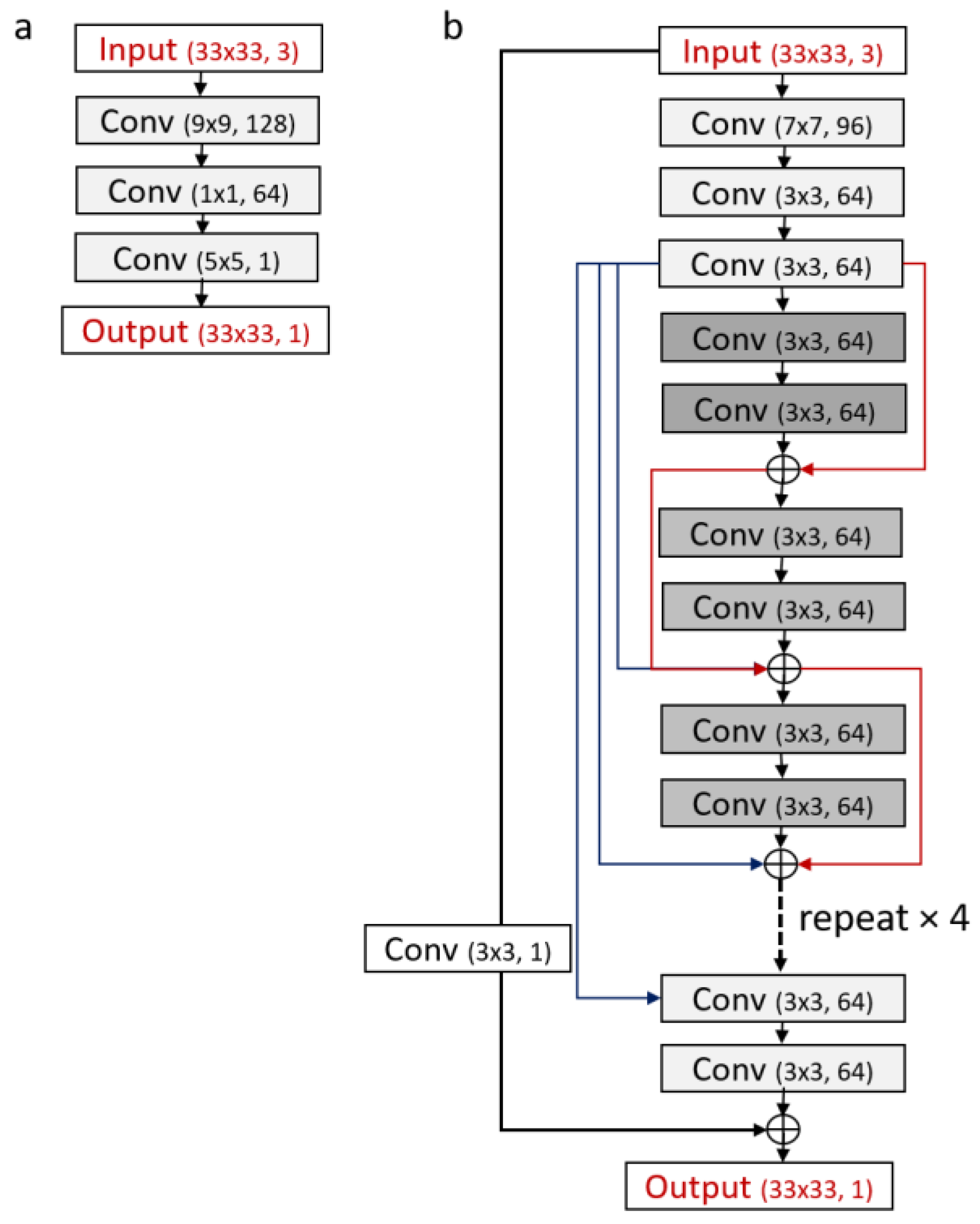
2.3. CNN Super-Resolution Models

There are countless configurations for network architectures that could be employed and will likely remain an area of significant future research. Although network design is important, for the purpose of this study we only tested two configurations. We tested the SRCNN of Dong et al. [10] because it is efficient with only 41,089 parameters and has shown good results (Figure 2A). We also apply a deeper architecture using residual learning, deep connectivity, and residual connections in attempt to integrate some of the latest improvements in the field (DCR_SRCNN). In initial exploratory analysis we tested numerous configurations of which the best was kept. We settled on the 20-layer configuration shown in Figure 2B inspired by Tai et al. [21]. This is a large network with 993,373 total parameters. The rectilinear unit was used for all activations. To improve generalization, least squares (L2) weight regularization was added to the third and second last layers of the network with a weight of 0.0001. Regularization was only applied to the last layers to avoid reducing the learning potential in the lower network layers. Input image size was 33 by 33 pixels. This size was selected to capture the spatial variation in the image while keeping the size small for computational efficiency. Filter sizes were 3 by 3, except for the first convolution layer where a 7 by 7 was used. The output features from each convolution layer was 64, except for the first layer which output 96. Also, the convolution layer for the residual learning objective output one result which essentially converted the input three band image to a single band.

We trained a model for each study site to allow for regional optimization. For training, the mean squared error loss function for the pixelwise comparison of the predicted and Sentinel-2 image was used with the Adam optimization method. This optimization method has been shown to provide an efficient and stable solution [35] and has been used in other CNN based super-resolution studies [18,25]. Early stopping criteria was applied, where if the loss did not improve in 10 epochs, training stopped. The total number of epochs was set at 80 with a batch size of 125. For all networks the input was the red, near-infrared (NIR), and short-wave infrared (SWIR, 1.55–1.75 µm) bands. Output, was a single band, either the red, NIR, or SWIR. All bands were input as spatial properties between bands were expected to provide useful information for determining specific spatial transforms. To allow for the greatest possible learning potential, a model was developed for each band. To focus the learning on the spatial properties between the samples, the mean of the Sentinel-2 image was adjusted to match the Landsat image.

All models were trained on a NVIDIA GeForce 1080 Ti GPU. Training time took approximately 2 days for the deep network for each study site and less than half this time for the shallow network.

3. Results

3.1. Hold-Out Accuracy

The results for the hold-out samples show that the DCR_SRCNN provided the best results across all study areas (

Table 2. Hold-out performance metrics.

Region	Method	Band	MEAN	STD	ME	MAE	STDE	P5E	P95E	SSIMm	SSIMs	CORm	CORs
Boreal forest	No Transform	Red	323	166	−0.88	36.50	63.14	−77.00	76.00	0.965	0.037	0.746	0.139
Boreal forest	No Transform	NIR	2050	720	−1.40	201.79	292.76	−450.00	469.00	0.827	0.085	0.803	0.110
Boreal forest	No Transform	SWIR	1247	428	−0.66	96.45	152.28	−225.00	219.00	0.915	0.075	0.852	0.122
Boreal forest	SRCNN	Red	323	166	−0.84	31.45	54.02	−62.03	67.86	0.973	0.029	0.794	0.139
Boreal forest	SRCNN	NIR	2050	720	4.76	167.19	240.25	−365.91	384.17	0.875	0.078	0.853	0.104
Boreal forest	SRCNN	SWIR	1247	428	−3.73	72.95	107.91	−160.51	166.31	0.942	0.063	0.895	0.118
Boreal forest	DCR_SRCNN	Red	323	166	3.95	28.36	42.50	−54.50	65.81	0.978	0.017	0.811	0.131
Boreal forest	DCR_SRCNN	NIR	2050	720	−8.66	141.01	195.48	−322.54	301.10	0.904	0.059	0.881	0.085
Boreal forest	DCR_SRCNN	SWIR	1247	428	5.72	49.00	69.94	−98.04	116.91	0.967	0.033	0.931	0.084
Tundra	No Transform	Red	1013	720	0.49	110.46	190.91	−240.00	263.00	0.875	0.069	0.784	0.098
Tundra	No Transform	NIR	1948	909	−0.66	163.53	258.55	−379.00	373.00	0.845	0.065	0.804	0.090
Tundra	No Transform	SWIR	2363	1449	2.58	184.42	314.71	−445.00	447.00	0.893	0.056	0.864	0.082
Tundra	SRCNN	Red	1013	718	−2.18	72.42	116.81	−161.39	160.70	0.943	0.037	0.885	0.078
Tundra	SRCNN	NIR	1948	908	8.23	103.97	151.04	−222.45	242.11	0.934	0.041	0.912	0.066
Tundra	SRCNN	SWIR	2363	1446	−0.34	99.10	154.68	−229.38	234.23	0.961	0.042	0.948	0.075
Tundra	DCR_SRCNN	Red	1013	718	9.23	62.935	93.99	−123.38	158.16	0.954	0.027	0.900	0.072
Tundra	DCR_SRCNN	NIR	1948	908	−5.24	85.713	118.71	−196.30	185.54	0.950	0.032	0.931	0.058
Tundra	DCR_SRCNN	SWIR	2363	1447	6.45	59.619	85.33	−129.24	142.42	0.980	0.022	0.969	0.060
Cropland/Woodland	No Transform	Red	318	253	−1.16	61.43	123.19	−149.00	170.00	0.899	0.107	0.644	0.177
Cropland/Woodland	No Transform	NIR	3325	1256	−12.73	319.87	441.58	−714.00	684.00	0.741	0.126	0.755	0.173
Cropland/Woodland	No Transform	SWIR	1582	605	−4.43	123.88	187.29	−291.00	278.00	0.869	0.112	0.773	0.118
Cropland/Woodland	SRCNN	Red	318	253	−0.41	52.65	101.73	−129.22	142.18	0.928	0.083	0.719	0.181
Cropland/Woodland	SRCNN	NIR	3325	1256	0.24	258.85	351.04	−563.76	569.60	0.830	0.112	0.819	0.160
Cropland/Woodland	SRCNN	SWIR	1582	605	−0.79	89.03	134.10	−194.72	207.90	0.913	0.099	0.874	0.172
Cropland/Woodland	DCR_SRCNN	Red	318	253	4.09	45.465	82.76	−103.66	123.95	0.945	0.057	0.748	0.173
Cropland/Woodland	DCR_SRCNN	NIR	3325	1256	28.70	232.460	312.05	−475.67	541.73	0.860	0.089	0.845	0.142
Cropland/Woodland	DCR_SRCNN	SWIR	1582	605	13.58	66.388	93.63	−127.05	164.15	0.948	0.052	0.909	0.134

MEAN—observed sample mean, STD—observed sample standard deviation, ME—mean error, MAE—mean absolute error, STDE—error standard deviation, P5E—5th percentile error, P95E—95th percentile error, SSIMm—mean SSIM, SSIMs—standard deviation SSIM, CORm—mean spatial correlation, CORs—standard deviation of spatial correlation.

). However, both methods showed marked improvement relative to applying no transformation for all the key metrics (MAE, SSIM, and spatial correlation). The MAE error is an informative measure as it is in standard reflectance units, but it is related to the mean of the sample, with a larger mean reflectance resulting in larger MAE. Further, the MAE can produce the same value for very different image qualities [33]. Spatial correlation is not related to the mean reflectance and gives a good indication of the spatial agreement and thus the spatial enhancement. However, it is influenced by the data range, with a reduce range producing a lower correlation [36]. SSIM essentially incorporates the MAE and spatial correlation measures in addition to image contrast. It is related to the sample mean reflectance, but to a much lesser degree than the MAE. It is important to recognize these limitations in interpreting the results when comparing bands.

Of the bands, the NIR consistently had the higher MAE and lower SSIM values regardless of the transformation. This is related to the high reflectance of the NIR band and associated larger variance. The SWIR, also had high reflectance for the tundra study site, but in contrast had low MAE and higher SSIM values. This was related to the native 20 m spatial resolution of the SWIR band in Sentinel-2, which results in greater initial similarity with Landsat compared to the 10 m bands. The spatial correlation showed that the red band had consistently lower values which was caused by the smaller reflectance range and atmospheric noise.

Of the study areas, the cropland/woodland showed the lowest performance due to change between the images despite efforts to reduce it. Change was also a potential factor in the boreal forest study site, but to a much lesser degree. The best results, were found for the northern tundra study area and was attributed to little change between images and less overall complexity of the land surface relative to the 10 m target resolution. Figure 3 provides an example image result of a residential area surrounded by mixed boreal forest conditions. It provides a good indication of the improvement that can be obtained. Figure 4 shows the enhancement by band for a mixed forest area with some industrial development. As evident from Figure 4, the NIR and red bands are more enhanced compared to the SWIR as expected. The coarse texture within the cover types is of interest and could prove useful for improving land cover discrimination or for biophysical retrieval as canopy variability or structure appears to be enhanced.

3.2. Spatial Extension Accuracy

The spatial extension accuracy shows similar or slightly reduced performance relative to the hold-out (

Table 3. Spatial extension performance metrics.

Region	Method	Band	MEAN	STD	ME	MAE	STDE	P5E	P95E	SSIMm	SSIMs	CORm	CORs
Boreal forest	No Transform	Red	336	114	−0.53	26.17	41.53	−54.00	55.00	0.977	0.024	0.775	0.142
Boreal forest	No Transform	NIR	2084	921	−0.69	143.96	211.10	−317.00	332.00	0.876	0.059	0.820	0.161
Boreal forest	No Transform	SWIR	1420	524	−1.10	49.94	77.52	−116.00	114.00	0.955	0.024	0.880	0.166
Boreal forest	SRCNN	Red	336	114	4.48	24.73	39.58	−46.10	56.61	0.979	0.025	0.791	0.162
Boreal forest	SRCNN	NIR	2084	921	−3.57	126.70	182.72	−277.60	289.22	0.903	0.053	0.847	0.173
Boreal forest	SRCNN	SWIR	1420	524	−12.31	50.14	73.00	−111.35	110.59	0.969	0.025	0.902	0.177
Boreal forest	DCR_SRCNN	Red	336	114	−0.37	24.23	37.80	−42.17	57.03	0.981	0.020	0.807	0.152
Boreal forest	DCR_SRCNN	NIR	2084	921	1.20	122.82	176.15	−280.86	268.82	0.910	0.051	0.853	0.166
Boreal forest	DCR_SRCNN	SWIR	1420	524	−0.47	51.35	82.06	−116.80	129.43	0.961	0.029	0.885	0.176
Tundra	No Transform	Red	1500	962	1.74	148.04	256.00	−346.00	353.00	0.865	0.112	0.820	0.120
Tundra	No Transform	NIR	2275	1132	1.06	170.06	283.40	−389.00	380.00	0.870	0.075	0.840	0.101
Tundra	No Transform	SWIR	3101	1701	0.37	223.58	413.35	−554.00	566.00	0.896	0.099	0.872	0.104
Tundra	SRCNN	Red	1500	962	−3.17	97.18	180.10	−205.83	208.11	0.936	0.106	0.909	0.110
Tundra	SRCNN	NIR	2275	1132	−3.57	101.92	158.59	−228.87	215.30	0.949	0.057	0.934	0.076
Tundra	SRCNN	SWIR	3101	1701	−8.22	129.31	251.22	−291.85	297.05	0.951	0.094	0.941	0.100
Tundra	DCR_SRCNN	Red	1500	962	12.78	92.82	176.46	−170.22	220.73	0.941	0.106	0.914	0.110
Tundra	DCR_SRCNN	NIR	2275	1132	−3.47	97.39	154.86	−218.60	209.26	0.952	0.056	0.937	0.073
Tundra	DCR_SRCNN	SWIR	3101	1701	5.69	138.25	271.00	−311.06	347.59	0.945	0.094	0.933	0.099
Cropland/Woodland	No Transform	Red	328	300	0.43	79.90	159.20	−184.00	231.00	0.864	0.109	0.640	0.176
Cropland/Woodland	No Transform	NIR	3632	1250	−10.51	354.13	490.97	−810.00	772.00	0.721	0.125	0.720	0.181
Cropland/Woodland	No Transform	SWIR	1628	543	−1.61	132.12	203.57	−299.00	303.00	0.848	0.118	0.770	0.200
Cropland/Woodland	SRCNN	Red	328	300	−2.44	69.22	135.09	−169.95	186.18	0.902	0.086	0.721	0.176
Cropland/Woodland	SRCNN	NIR	3632	1250	−6.12	304.61	419.01	−678.00	672.29	0.807	0.111	0.789	0.166
Cropland/Woodland	SRCNN	SWIR	1628	543	−1.43	104.11	157.00	−222.85	242.84	0.896	0.104	0.844	0.193
Cropland/Woodland	DCR_SRCNN	Red	328	300	4.41	69.81	139.20	−163.35	195.46	0.902	0.084	0.720	0.170
Cropland/Woodland	DCR_SRCNN	NIR	3632	1250	26.46	300.29	412.67	−630.31	695.18	0.816	0.110	0.797	0.161
Cropland/Woodland	DCR_SRCNN	SWIR	1628	543	14.42	89.49	141.21	−174.24	227.41	0.909	0.101	0.856	0.191

MEAN—observed sample mean, STD—observed sample standard deviation, ME—mean error, MAE—mean absolute error, STDE—error standard deviation, P5E—5th percentile error, P95E—95th percentile error, SSIMm—mean SSIM, SSIMs—standard deviation SSIM, CORm—mean spatial correlation, CORs—standard deviation of spatial correlation.

). Comparing the results for the two CNNs it is not evident that the deeper model made a sufficiently large improvement to warrant its greater computational complexity. This is likely caused by some overtraining and errors, due to temporal change, in the training and validation data which can reduce the sensitivity of the analysis.

The cropland study site showed the greatest difference relative to the hold-out results. The difference is in part related to the greater amount of agriculture in the extension sample. Due to the changes in crops for the 14 to 21-day difference between images, there were limited sampling opportunities and thus, the extension results did not perform as well. Croplands present a particular challenge for the approach as training data is limited by the highly dynamic nature of cropland environments with dramatic reflectance changes over a few days. With the Sentinel-2 constellation potentially more temporally coincident imagery will be captured to ensure suitable training. Otherwise spatial extension over greater distances may be required for large extent enhancements. The performance for bands suggests the same conclusion as the hold-out sample results.

3.3. Temporal Extension Accuracy

Temporal extension accuracy is an important aspect of the approach to determine if a trained network can be applied to enhance Landsat time series.

Table 4. Temporal extension performance metrics.

Region	Date	Band	No Transform		SRCNN		DCDR_SRCNN		No Transform		SRCNN		DCDR_SRCNN		No Transform		SRCNN		DCDR_SRCNN
			MAE	STDE	MAE	STDE	MAE	STDE	CORm	CORs	CORm	CORs	CORm	CORs	SSIMm	SSIMs	SSIMm	SSIMs	SSIMm	SSIMs
Boreal forest	1984_07_23	Red	43	65	39	61	36	59	0.406	0.267	0.443	0.279	0.454	0.277	0.925	0.096	0.934	0.098	0.936	0.097
Boreal forest	1984_07_23	NIR	275	374	272	373	273	374	0.515	0.251	0.548	0.247	0.559	0.246	0.575	0.199	0.609	0.205	0.620	0.206
Boreal forest	1984_07_23	SWIR	136	186	134	183	129	179	0.488	0.288	0.527	0.295	0.538	0.298	0.702	0.179	0.721	0.184	0.726	0.184
Boreal forest	1997_08_28	Red	42	65	36	59	34	58	0.507	0.223	0.563	0.238	0.576	0.239	0.932	0.087	0.942	0.090	0.945	0.089
Boreal forest	1997_08_28	NIR	269	370	261	363	259	360	0.572	0.221	0.628	0.212	0.643	0.207	0.618	0.188	0.669	0.185	0.682	0.180
Boreal forest	1997_08_28	SWIR	120	169	116	164	111	160	0.644	0.233	0.686	0.240	0.695	0.241	0.779	0.156	0.801	0.160	0.807	0.160
Boreal forest	2011_07_20	Red	33	52	28	47	27	46	0.674	0.122	0.738	0.114	0.752	0.107	0.959	0.042	0.966	0.046	0.968	0.044
Boreal forest	2011_07_20	NIR	199	273	174	241	169	235	0.798	0.080	0.839	0.072	0.848	0.071	0.784	0.077	0.845	0.066	0.860	0.064
Boreal forest	2011_07_20	SWIR	80	114	75	107	64	92	0.855	0.061	0.899	0.057	0.913	0.057	0.907	0.049	0.932	0.048	0.940	0.048
Cropland/Woodland	1987_08_11	Red	65	121	64	126	69	127	0.527	0.229	0.576	0.236	0.582	0.243	0.866	0.125	0.870	0.124	0.870	0.122
Cropland/Woodland	1987_08_11	NIR	459	606	415	556	400	541	0.679	0.233	0.722	0.214	0.732	0.217	0.632	0.203	0.724	0.198	0.737	0.202
Cropland/Woodland	1987_08_11	SWIR	176	241	167	225	146	207	0.750	0.222	0.781	0.224	0.787	0.228	0.785	0.149	0.820	0.157	0.828	0.162
Cropland/Woodland	2002_07_30	Red	57	107	55	109	58	107	0.611	0.192	0.655	0.198	0.663	0.200	0.891	0.102	0.897	0.103	0.900	0.098
Cropland/Woodland	2002_07_30	NIR	414	551	374	505	364	499	0.763	0.166	0.796	0.160	0.805	0.159	0.725	0.152	0.799	0.150	0.807	0.152
Cropland/Woodland	2002_07_30	SWIR	149	206	143	189	119	184	0.819	0.158	0.846	0.171	0.853	0.172	0.841	0.105	0.872	0.121	0.880	0.123
Cropland/Woodland	2007_08_20	Red	57	105	47	88	46	86	0.638	0.149	0.723	0.132	0.745	0.128	0.897	0.094	0.926	0.065	0.931	0.061
Cropland/Woodland	2007_08_20	NIR	433	574	317	420	300	404	0.805	0.115	0.848	0.100	0.857	0.100	0.684	0.110	0.835	0.098	0.853	0.100
Cropland/Woodland	2007_08_20	SWIR	135	188	105	148	93	131	0.875	0.077	0.915	0.069	0.924	0.069	0.880	0.050	0.925	0.055	0.936	0.054
Tundra	1987_08_01	Red	91	136	79	114	78	111	0.749	0.142	0.804	0.134	0.806	0.135	0.877	0.067	0.906	0.061	0.908	0.061
Tundra	1987_08_01	NIR	155	230	126	180	127	183	0.813	0.100	0.878	0.088	0.878	0.090	0.853	0.067	0.907	0.057	0.907	0.058
Tundra	1987_08_01	SWIR	207	312	154	226	131	190	0.851	0.092	0.907	0.083	0.915	0.080	0.870	0.075	0.918	0.066	0.925	0.067
Tundra	1994_08_04	Red	91	135	78	111	77	110	0.757	0.142	0.810	0.135	0.811	0.137	0.875	0.067	0.907	0.060	0.907	0.060
Tundra	1994_08_04	NIR	157	230	121	172	119	171	0.816	0.107	0.881	0.097	0.882	0.095	0.846	0.078	0.906	0.067	0.908	0.065
Tundra	1994_08_04	SWIR	190	294	142	211	119	176	0.847	0.117	0.907	0.103	0.916	0.099	0.872	0.092	0.921	0.081	0.928	0.078
Tundra	2010_07_15	Red	83	139	65	98	64	94	0.801	0.103	0.876	0.080	0.881	0.078	0.895	0.076	0.939	0.045	0.942	0.041
Tundra	2010_07_15	NIR	150	226	106	150	103	148	0.829	0.085	0.910	0.063	0.913	0.061	0.859	0.063	0.930	0.042	0.934	0.040
Tundra	2010_07_15	SWIR	190	292	133	195	104	152	0.861	0.082	0.929	0.059	0.941	0.054	0.883	0.063	0.939	0.046	0.950	0.043

MAE—mean absolute error, STDE—error standard deviation, SSIMm—mean SSIM, SSIMs—standard deviation SSIM, CORm—mean spatial correlation, CORs—standard deviation of spatial correlation.

provides the temporal extension results. These at first glance appear to be low, particularly the spatial correlation, but assessment of temporal extension is fraught with difficulties. The main challenge is that no-changes areas do not exist in terms of image reflectance’s. For the purposes of land cover, no-change can be identified, but in comparing imagery between dates there are always changes due to canopy dynamics, annual changes in canopy configuration, moisture content, residual atmosphere effects, etc. that do not change the land cover, but alter reflectance’s for a cover type. Thus, in interpreting these results it is important to note that the sensitivity and accuracy is influenced by this effect. Irrespective, in all cases the metrics were improved with either CNN.

The temporal effect is clearly seen in the boreal forest and cropland/woodland study sites, where the performance metrics all improve as the image date gets closer to the Sentinel-2 image used as a reference. The tundra study area is likely the most informative as changes are subtler, less frequent and the vegetation structure is small relative to the image spatial resolution. Thus, these results are more indicative of the temporal extension capacity. The shallow network performed similarly to the deep network but with slightly reduced magnitude across all metrics of approximately 1%. The small difference is in part a result of temporal changes in the test data which reduces the sensitivity of the analysis. This is similar to the spatial extension results, but is expected to be more significant.

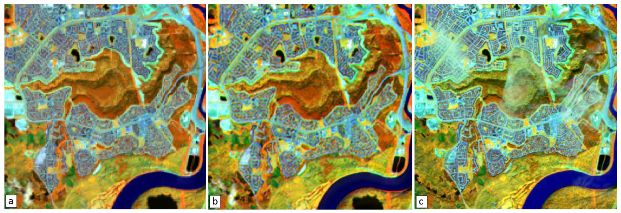
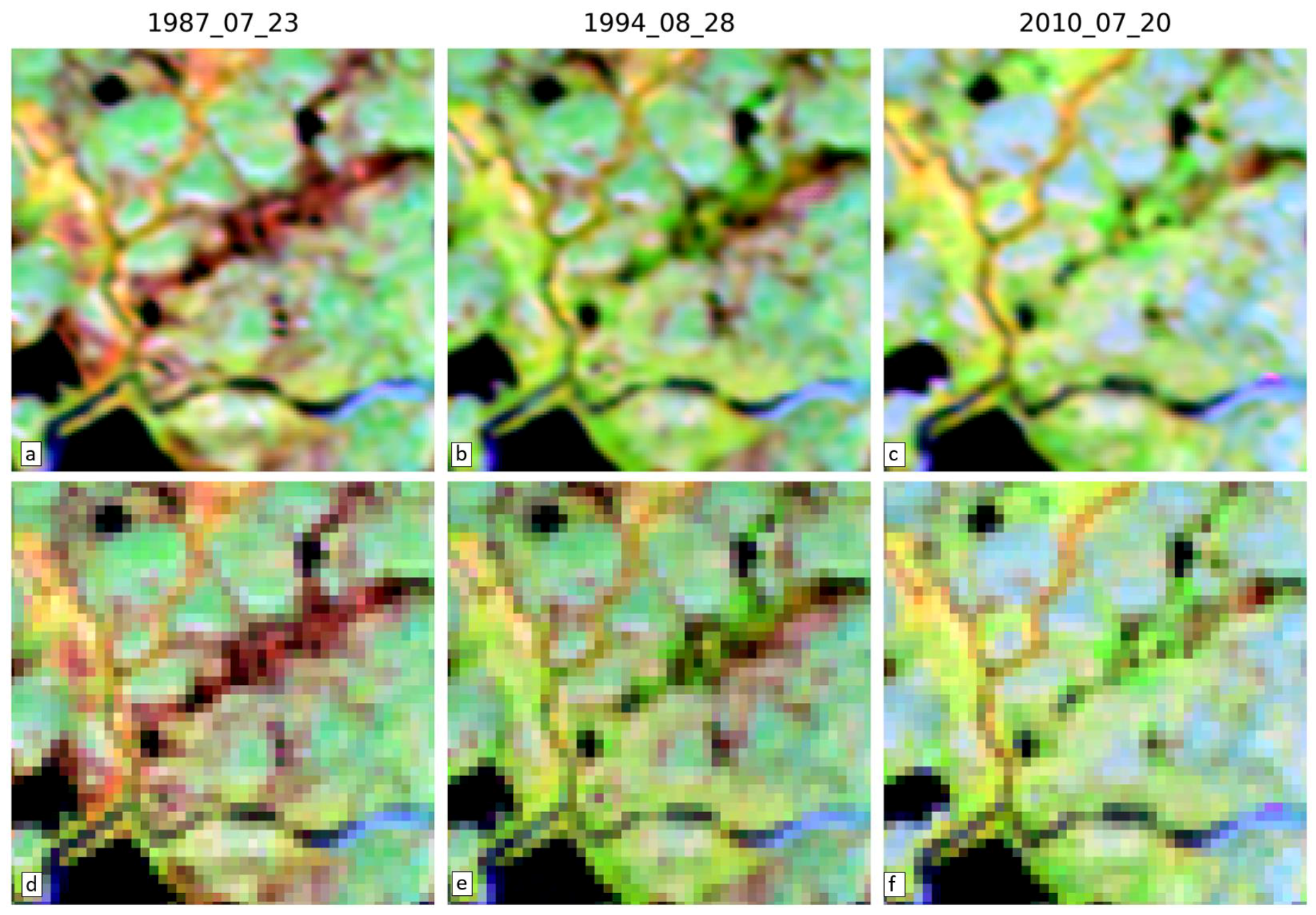
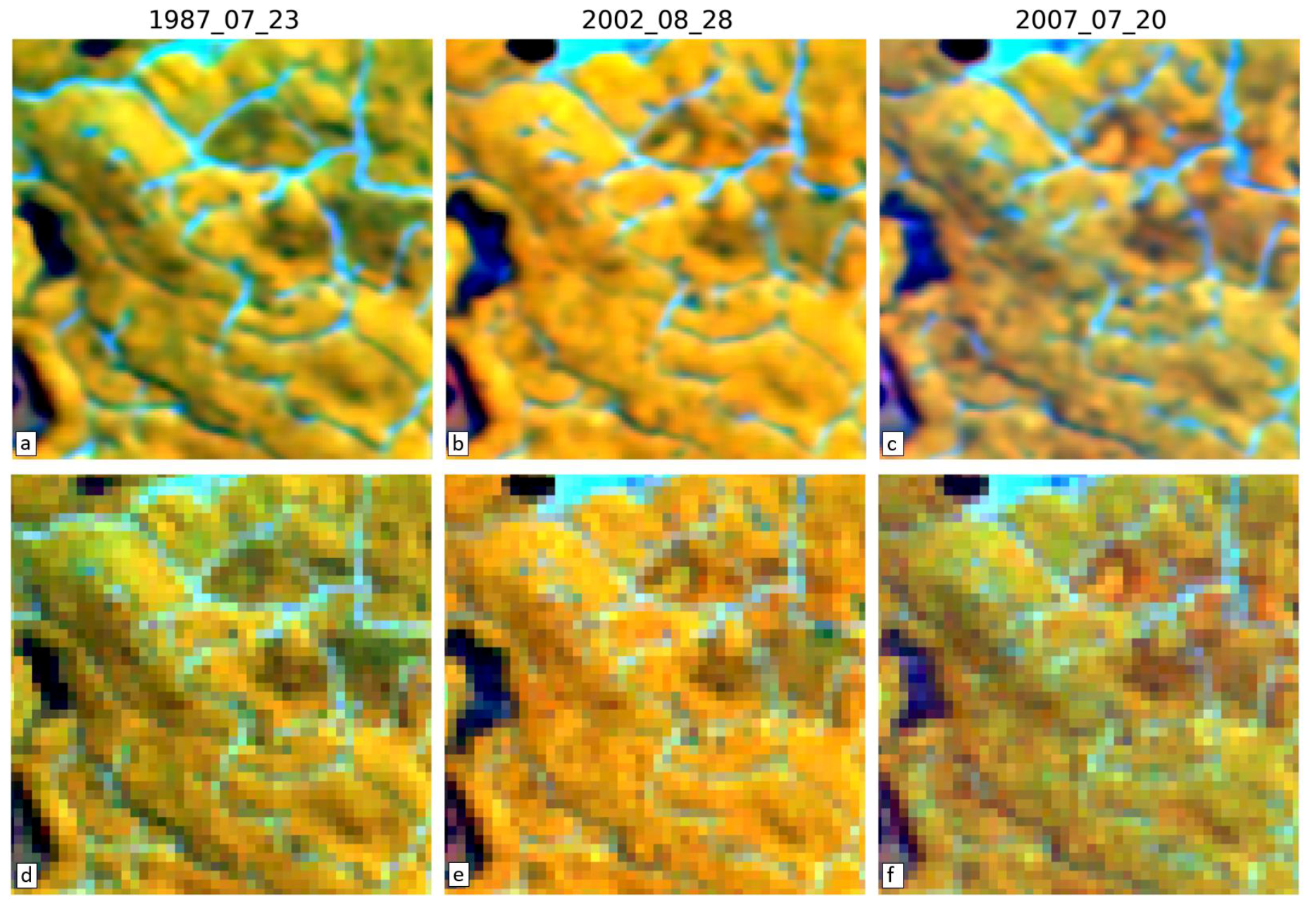
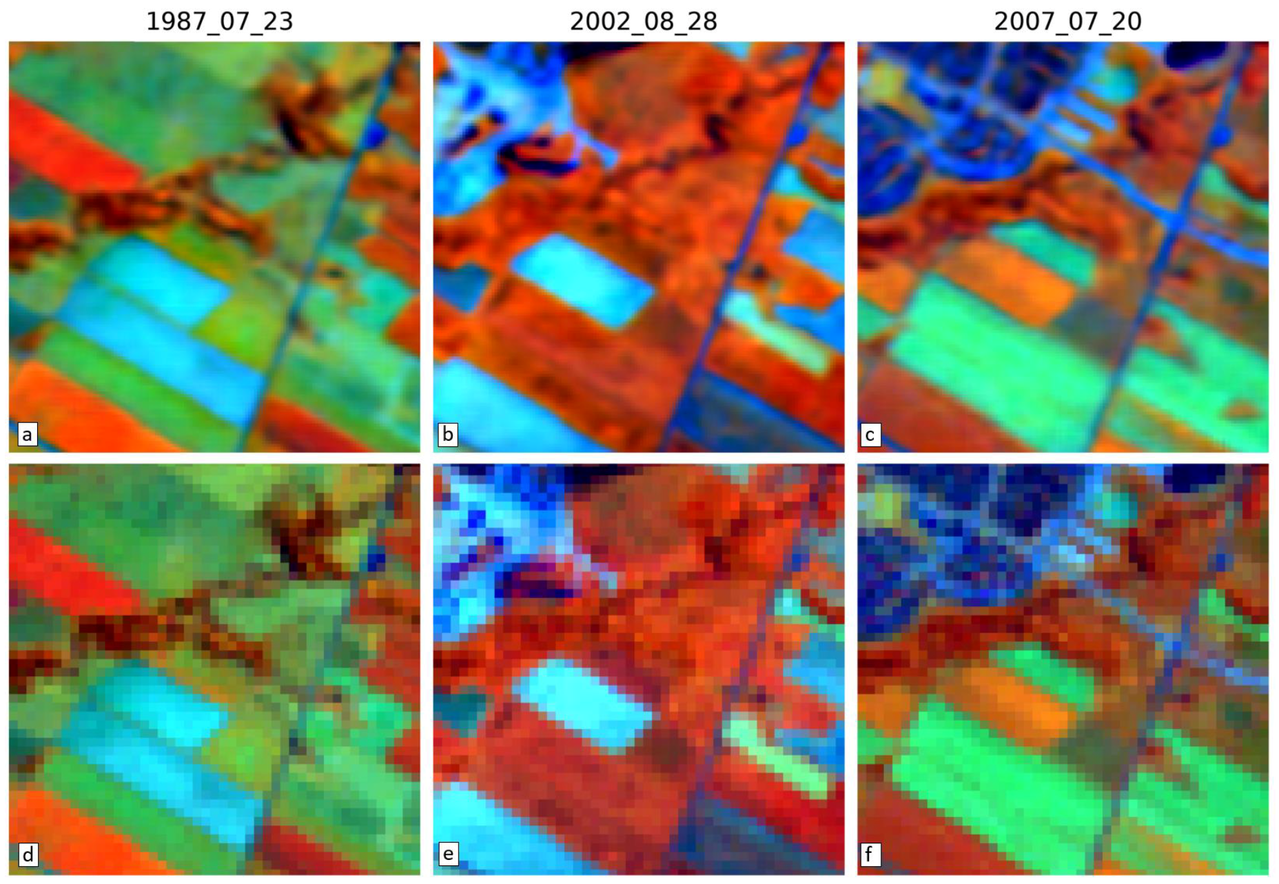
3.4. Visual Assessment

Visual assessment provides the more convincing evidence as the nature of the enhancement can be clearly recognized and artifacts readily identified. Here, we provide several examples of enhanced images for the different landscape environments and over multiple years in Figure 5, Figure 6, Figure 7 and Figure 8. In all examples, boundaries are clearer between cover types, linear features are more apparent, within cover textures are enhanced, and the spatial structure overall is clearer. There are also no major artifacts created within images or between image dates. Although, some speckle is introduced in a few cases. In Figure 5, the spatial structure of forest gaps or leaf area gradients appear to be enhanced. This is most evident in the 2011 imagery as fire damage has resulted in greater canopy variability. This could possibly lead to improvements in biophysical retrievals or habitat analysis, but requires further study. Figure 6 shows the northern tundra example, it more clearly defines drainage patterns and water bodies. Figure 7 shows area of trails and roads that have become much more apparent in the broadleaf forest area. This highlights the potential of the approach to better characterize edges which could enhance land cover-based landscape metrics. The final example, Figure 8 shows an area of cropland where the boundaries between crop areas and roads has been improved.

4. Discussion

In this research we show that CNN super-resolution can spatially enhance Landsat imagery and can be applied to historical peak growing season time series that could improve land cover and land cover change applications or possibly biophysical parameter retrievals. However, future research needs to specifically evaluate the improvement for a given application with this type of enhancement. This is important to determine if the approach is only suitable for visual enhancement or some types of quantitative analysis. Here, we show that boundaries between land covers and linear features are improved and likely would influence landscape metrics derived from land cover data. There are also textural enhancements that need to be explored as a means to improve information extraction applications.

The SSIM values obtained compare well with other studies achieving values in the range of 0.86 to 0.97, similar to what is achieved in benchmark image databases for an upscaling factor of three [21]. However, in most studies, images are degraded from an initial high-resolution image and thus the only differences between the fine and coarse images used for training is resolution. This was not the case in this research as there were several additional factors other than resolution and included changes or differences in land cover, canopy structure, phenology, moisture, residual atmosphere effects, sun-sensor geometry, sensor spectral response functions, and residual geolocation error. These factors need to be considered in examining the results as they reduce sensitively of the analysis. More importantly this can cause models to learn these differences resulting in reduced spatial and temporal generalization performance. For remote sensing data, Collins et al. [25] report SSIM values greater than 0.98. This is the result of using coinstantaneous images avoiding many of the factors listed above. It is also due to the upscaling factor of 2. In this study the upscaling factors were 3 for the red and near-infrared and 1.5 for the shortwave. The inferior result obtained here for the SWIR suggests that the difference is largely related to temporal variation. However, Collins et al. do not report band specific values.

It also of interest to compare the effects of using a more complex network. In Collins et al., going from shallow to wider and deeper improved the SSIM by 0.0035. In this research we also see only a small increase with the more complex deeper network, improving by about 0.006 on average for both the spatial and temporal extension. Thus, as with other SR research finding the optimal balance between model complexity and performance will be an important aspect of future research. In this regard, the effective resolution of the spatial enhancement needs to be determined. That is, we do not propose that the CCN learns a true 10 m resolution result. Future efforts need to quantify the effective resolution to avoid storage and processing redundancy.

Other approaches to assess performance were considered, such as comparison with other high spatial-resolution more temporally coincident images. However, finding such images is challenging for many regions such as the north and where suitable cloud free pairs are difficult to obtain within a few days of acquisition. This may be possible for the visible and NIR bands, but there are few higher spatial resolution sensors that capture the SWIR band for comparison and development with Landsat-5. SPOT-5 imagery is a suitable option, but it was not available for this analysis and establishing an extensive database would be costly. Despite this, the visual assessment shows that the trained networks were able to enhance the spatial properties of the images through time without introducing any strong artifacts.

For large regional implementation, spatial extension over greater distances may be required. For distances less than 100 km, the CNNs appeared to generalize well. However, to effectively train Landsat-5, larger distances may be required as suitable training locations would be limited to areas with little change or with suitable SPOT-5 images. There are several mechanisms to further enhance the generalization of the CNNs that need to be explored in future research such as optimizing network size, increasing weight regularization, batch normalization, and data augmentation. The deep network employed in this research was selected to provide an indication of the upper bound on the enhancement potential. The expectation was that a comprise between the deep and shallow network would be more effective for implementation. In this work we also included weight regularization for the last layers in the network and thus better generalization may be obtained by applying regularizing to additional layers and increasing the weight. In this research we did not use batch normalization as it was found to slightly reduce results in Liang et al. [37]. However, for spatial and temporal extension this may not be the case and requires further investigation. We also did not use data augmentation as our sample sizes were large, except for retraining of Landsat-5 for the identified no-change areas. In this case, data augmentation could provide an advantage. Data augmentation also provides an alternative training strategy, where more stringent criteria for selecting samples could be applied and data augmentation used to offset the reduced sample size. Improvements in the training data is expected to improve performance.

5. Conclusions

In this research we tested a shallow and deep CNN for the purpose of super-resolution enhancement of the Landsat archive trained from Sentinel-2 images. Results show improvement in spatial properties of the enhanced imagery and good potential for spatial and temporal extension of the CNNs developed in all the study areas. The deep CCN showed better performance, but it is not clear if it is worth the additional computational complexity and memory requirements. As research in CNN super-resolution for other applications has shown, it is possible to achieve similar performance with simpler configurations. Significant advancement of this approach is expected with progression in network design, training data sources, sampling strategies, and improved regularization. Despite this, the models developed here were effective at enhancing image spatial structure which is expected to improve land cover and land cover change applications.

References

1. Zhu, Z.; Woodcock, C.E.; Olofsson, P. Continuous monitoring of forest disturbance using all available Landsat imagery. Remote Sens. Environ. 2012, 122, 75–91. [Google Scholar] [CrossRef]
2. Zhu, Z.; Woodcock, C.E. Continuous change detection and classification of land cover using all available Landsat data. Remote Sens. Environ. 2014, 144, 152–171. [Google Scholar] [CrossRef]
3. Pouliot, D.; Latifovic, R. Reconstruction of Landsat time series in the presence of irregular and sparse observations: Development and assessment in north-eastern Alberta, Canada. Remote Sens. Environ. 2017. [Google Scholar] [CrossRef]
4. Song, H.; Huang, B.; Liu, Q.; Zhang, K. Improving the Spatial Resolution of Landsat TM/ETM+ Through Fusion with SPOT5. IEEE Trans. Geosci. Remote Sens. 2014, 53, 1195–1204. [Google Scholar] [CrossRef]
5. Grochala, A.; Kedzierski, M. A method of panchromatic image modification for satellite imagery data fusion. Remote Sens. 2017, 9, 639. [Google Scholar] [CrossRef]
6. Li, Z.; Zhang, K.H.; Roy, P.D.; Yan, L.; Huang, H.; Li, J. Landsat 15-m Panchromatic-Assisted Downscaling (LPAD) of the 30-m Reflective Wavelength Bands to Sentinel-2 20-m Resolution. Remote Sens. 2017, 9, 755. [Google Scholar] [CrossRef]
7. Masi, G.; Cozzolino, D.; Verdoliva, L.; Scarpa, G. Pansharpening by convolutional neural networks. Remote Sens. 2016, 8. [Google Scholar] [CrossRef]
8. Gilbertson, J.K.; Kemp, J.; van Niekerk, A. Effect of pan-sharpening multi-temporal Landsat 8 imagery for crop type differentiation using different classification techniques. Comput. Electron. Agric. 2017, 134, 151–159. [Google Scholar] [CrossRef]
9. Joshi, N.; Baumann, M.; Ehammer, A.; Fensholt, R.; Grogan, K.; Hostert, P.; Jepsen, M.R.; Kuemmerle, T.; Meyfroidt, P.; Mitchard, E.T.A.; et al. A review of the application of optical and radar remote sensing data fusion to land use mapping and monitoring. Remote Sens. 2016, 8, 70. [Google Scholar] [CrossRef]
10. Dong, C.; Loy, C.C.; He, K.; Tang, X. Learning deep convolutional networks for image super resolution. In Proceedings of the European Conference on Computer Vision, Athens, Greece, 11–13 November 2015. [Google Scholar]
11. Krizhevsky, A.; Sutskever, I.; Hinton, G.E. ImageNet Classification with Deep Convolutional Neural Networks. Adv. Neural Inf. Process. Syst. 2012, 1–9. [Google Scholar] [CrossRef]
12. Hu, F.; Xia, G.-S.; Hu, J.; Zhang, L. Transferring Deep Convolutional Neural Networks for the Scene Classification of High-Resolution Remote Sensing Imagery. Remote Sens. 2015, 7, 14680–14707. [Google Scholar] [CrossRef]
13. Krizhevsky, A. Learning Multiple Layers of Features from Tiny Images; University of Toronto: Toronto, ON, Canada, 2009; pp. 1–60. [Google Scholar]
14. Russakovsky, O.; Deng, J.; Su, H.; Krause, J.; Satheesh, S.; Ma, S.; Huang, Z.; Karpathy, A.; Khosla, A.; Bernstein, M.; et al. ImageNet Large Scale Visual Recognition Challenge. Int. J. Comput. Vis. 2015, 115, 211–252. [Google Scholar] [CrossRef]
15. Kim, J.; Lee, J.K.; Lee, K.M. Deeply-Recursive Convolutional Network for Image Super-Resolution. arXiv, 2015; arXiv:1511.04491. [Google Scholar]
16. Kim, J.; Lee, J.K.; Lee, K.M. Accurate Image Super-Resolution Using Very Deep Convolutional Networks. arXiv, 2016; arXiv:1511.04587. [Google Scholar]
17. Svoboda, P.; Hradis, M.; Barina, D.; Zemcik, P. Compression Artifacts Removal Using Convolutional Neural Networks. arXiv, 2016; arXiv:1605.00366. [Google Scholar]
18. Mao, X.-J.; Shen, C.; Yang, Y.-B. Image Restoration using very Deep Convolutional Encoder-Decoder Networks with Symmetric Skip Connections. arXiv, 2016; arXiv:1603.09056. [Google Scholar]
19. Wang, L.; Huang, Z.; Gong, Y.; Pan, C. Ensemble based deep networks for image super-resolution. Pattern Recognit. 2017, 68, 191–198. [Google Scholar] [CrossRef]
20. Shi, W.; Caballero, J.; Huszár, F.; Totz, J.; Aitken, A.P.; Bishop, R.; Rueckert, D.; Wang, Z. Real-Time Single Image and Video Super-Resolution Using an Efficient Sub-Pixel Convolutional Neural Network. arXiv, 2016; arXiv:1609.05158. [Google Scholar]
21. Tai, Y.; Yang, J.; Liu, X. Image Super-Resolution via Deep Recursive Residual Network. In Proceedings of the IEEE Conference on Computer Vision and Pattern Recognition, Honolulu, HI, USA, 21–26 July 2017; pp. 3147–3155. [Google Scholar] [CrossRef]
22. He, K.; Zhang, X.; Ren, S.; Sun, J. Deep Residual Learning for Image Recognition. arXiv, 2015; arXiv:1512.03385. [Google Scholar]
23. Zagoruyko, S.; Komodakis, N. Wide Residual Networks. arXiv, 2016; arXiv:1605.07146. [Google Scholar]
24. Xie, S.; Girshick, R.; Dollár, P.; Tu, Z.; He, K. Aggregated Residual Transformations for Deep Neural Networks. arXiv, 2017; arXiv:1611.05431. [Google Scholar]
25. Collins, C.B.; Beck, J.M.; Bridges, S.M.; Rushing, J.A.; Graves, S.J. Deep Learning for Multisensor Image Resolution Enhancement. In Proceedings of the 1st Workshop on Artificial Intelligence and Deep Learning for Geographic Knowledge Discovery, Redondo Beach, CA, USA, 7 November 2017; pp. 37–44. [Google Scholar] [CrossRef]
26. Latifovic, R.; Pouliot, D.; Olthof, I. Circa 2010 Land Cover of Canada: Local Optimization Methodology and Product Development. Remote Sens. 2017, 9, 1098. [Google Scholar] [CrossRef]
27. Mueller-Wilm, U.M. S2 MPC Sen2Cor Configuration and User Manual; European Space Agency: Paris, France, 2017. [Google Scholar]
28. Storey, J.; Roy, D.P.; Masek, J.; Gascon, F.; Dwyer, J.; Choate, M. A note on the temporary misregistration of Landsat-8 Operational Land Imager (OLI) and Sentinel-2 Multi Spectral Instrument (MSI) imagery. Remote Sens. Environ. 2016, 186, 121–122. [Google Scholar] [CrossRef]
29. Storey, J.; Choate, M.; Rengarajan, R.; Lubke, M. Landsat-8/Sentinel-2 Registration Accuracy and Improvement Status; United States Geological Survey: Reston, VA, USA, 2017.
30. Latifovic, R.; Pouliot, D.; Sun, L.; Schwarz, J.; Parkinson, W. Moderate Resolution Time Series Data Management and Analysis: Automated Large Area Mosaicking and Quality Control; Natural Resources Canada: Ottawa, ON, Canada, 2015. [Google Scholar] [CrossRef]
31. United States Geological Survey. USGS Product Guide Landsat 8 Surface Reflectance Code (LaSRC) Product; United States Geological Survey: Reston, VA, USA, 2017; pp. 1–38.
32. Lambin, E.F.; Strahlers, A.H. Change-vector analysis in multitemporal space: A tool to detect and categorize land-cover change processes using high temporal-resolution satellite data. Remote Sens. Environ. 1994, 48, 231–244. [Google Scholar] [CrossRef]
33. Wang, Z.; Bovik, A.C.; Sheikh, H.R.; Simoncelli, E.P. Image quality assessment: From error visibility to structural similarity. IEEE Trans. Image Process. 2004, 13, 600–612. [Google Scholar] [CrossRef] [PubMed]
34. Fernandes, R.; Leblanc, S.G. Parametric (modified least squares) and non-parametric (Theil-Sen) linear regressions for predicting biophysical parameters in the presence of measurement errors. Remote Sens. Environ. 2005, 95, 303–316. [Google Scholar] [CrossRef]
35. Ruder, S. An overview of gradient descent optimization algorithms. arXiv, 2016; arXiv:1609.04747. [Google Scholar]
36. Goodwin, L.D.; Leech, N.L. Understanding correlation: Factors that affect the size of r. J. Exp. Educ. 2006, 74, 249–266. [Google Scholar] [CrossRef]
37. Liang, Y.; Yang, Z.; Zhang, K.; He, Y.; Wang, J.; Zheng, N. Single Image Super-resolution with a Parameter Economic Residual-like Convolutional Neural Network. In Proceedings of the International Conference on Multimedia Modeling, Reykjavik, Iceland, 4–6 January 2017. [Google Scholar]
Figure 1. Study site locations and Landsat scene footprints.
Remotesensing 10 00394 g001
Figure 2. Configuration of the CNNs tested. (a) The SRCNN of Dong et al. [10]. (b) The deep residual and connected CNN developed. Red lines are residual blocks and blue lines are connections between residual blocks. Black line is the connection for the residual learning objective, which is put through a single convolution layer to convert the input three band image to a single band. The ⊕ symbol represents summation of the output activation layer elements.
Remotesensing 10 00394 g002
Figure 3. Examples results for a residential area surrounded by mixed boreal forest conditions; (a) Landsat image, (b) resolution enhanced, and (c) Sentinel-2 image. Displayed as red = NIR, green = SWIR, blue = red.
Remotesensing 10 00394 g003
Figure 4. Example results for each band for a mixed boreal forest with some industrial development; (a,d,g,j) Landsat image, (b,e,h,k) resolution enhanced, and (c,f,i,l) Sentinel-2 image. (ac) multi-band image displayed as red = NIR, green = SWIR, blue = red, (df) NIR, (gi) SWIR, (jl) red.
Remotesensing 10 00394 g004
Figure 5. Example temporal extension result for a boreal mixedwood forest. (ac) is the spatially enhanced result and (df) is the original Landsat.
Remotesensing 10 00394 g005
Figure 6. Example temporal extension result for a northern tundra area. (ac) is the spatially enhanced result and (df) is the original Landsat.
Remotesensing 10 00394 g006
Figure 7. Example temporal extension result for a broadleaf forestarea. (ac) is the spatially enhanced result and (df) is the original Landsat.
Remotesensing 10 00394 g007
Figure 8. Example temporal extension result for a cropland area. (ac) is the spatially enhanced result and (df) is the original Landsat.
Remotesensing 10 00394 g008