Empirical Algorithm for Significant Wave Height Retrieval from Wave Mode Data Provided by the Chinese Satellite Gaofen-3

Abstract

Gaofen-3 (GF-3), the first Chinese civil C-band synthetic aperture radar (SAR), was successfully launched by the China Academy of Space Technology on 10 August 2016. Among its 12 imaging modes, wave mode is designed to monitor the ocean surface waves over the open ocean. An empirical retrieval algorithm of significant wave height (SWH), termed Quad-Polarized C-band WAVE algorithm for GF-3 wave mode (QPCWAVE_GF3), is developed for quad-polarized SAR measurements from GF-3 in wave mode. QPCWAVE_GF3 model is built using six SAR image and spectrum related parameters. Based on a total of 2576 WaveWatch III (WW3) and GF-3 wave mode match-ups, 12 empirical coefficients of the model are determined for 6 incidence angle modes. The validation of the QPCWAVE_GF3 model is performed through comparisons against independent WW3 modelling hindcasts, and observations from altimeters and buoys from January to October in 2017. The assessment shows a good agreement with root mean square error from 0.5 m to 0.6 m, and scatter index around 20%. In particular, applications of the QPCWAVE_GF3 model in SWH estimation for two storm cases from GF-3 data in wave mode and Quad-Polarization Strip I mode are presented respectively. Results indicate that the proposed algorithm is suitable for SWH estimation from GF-3 wave mode and is promising for other similar data.

1. Introduction

Ocean surface wave measurements are valuable for various areas. Significant wave height (SWH) is one of the most important parameters for ocean wave observations. For decades, the space-borne synthetic aperture radars (SARs) have demonstrated the capability to provide ocean wave spectra and/or SWH at high spatial resolution under all weather conditions [1,2,3]. Especially, the so-called Wave Mode (WM), adopted by European SARs aboard ERS-1/2, Envisat, and recently launched Sentinel-1A/B, can provide information on ocean swells in open ocean and ice-covered regions at a global scale since 1991 [4,5,6,7]. The SAR WM products have been widely used in the various applications, such as ocean wave operational assimilation at weather centers [8], monitoring of swell propagation [5,6], and detection of crossing swells [9,10].

Traditionally, SAR SWH retrieval schemes fall into two categories. In the first set of methodologies, the principle of SWH retrieval is to integrate the directional ocean wave spectrum estimated from the SAR spectrum. However, the first-guess wave spectra or additional wind information are needed to invert the spectrum e.g., [11,12,13,14]; otherwise, the retrieved spectra and therefore SWH are restricted to the long wave regime [15]. In this context, the second type of scheme, called empirical algorithms, which do not require prior wave/wind information, has emerged over the last ten years. Similar to the Geophysical Model Functions (GMFs) used for SAR ocean wind measurements i.e., [16,17,18], the SAR SWH empirical models could estimate SWH directly from inputs computed from SAR images and/or SAR spectra. These include the C-band WAVE algorithm for ERS-2 wave mode (CWAVE_ERS) [19], C-band WAVE algorithm for Envisat wave mode (CWAVE_ENV) [20] and X-band WAVE algorithm (XWAVE) [21,22] developed by German Aerospace Center (DLR), C-band WAVE algorithm for Sentinel-1A wave mode (CWAVE_S1A) and CWAVE_Fnn [23] proposed by Institut Français de Recherche pour l’Exploitation de la Mer (IFREMER), and other empirical SWH retrieval attempts for SAR data provided by Envisat ASAR (Advanced Synthetic Aperture Radar) [24], Sentinel-1A [25,26], Radarsat-2 [27,28], and TerraSAR-X [29].

On 10 August 2016, the first Chinese civil multi-polarization SAR, the Gaofen-3 (GF-3) satellite, was successfully launched by the China Academy of Space Technology. The C-band (~5.3 GHz) GF-3 SAR is circling the Earth in a sun-synchronous orbit at a 755 km altitude with an orbit repeat cycle of about 29 days, and can operate in 12 imaging modes, including WM [30,31]. Recently, some initial efforts to estimate ocean surface winds and waves using GF-3 SAR data have been carried out, implying promising oceanic applications of the GF-3 SAR mission [32,33,34,35,36].

To date, although GF-3 is the first non-European satellite equipped with SAR WM, investigations on ocean wave retrieval from GF-3 focus mainly on data acquired in the Standard Strip or Quad-Polarization Strip I (QPSI) modes [33,34], instead of the unique working mode of WM. In fact, GF-3 WM is operating at different incident angles from those of C-band European SAR satellites equipped with WM, such as ERS-2, Envisat ASAR, and Sentinel-1 A/B, obstructing the direct adoption of existing empirical SWH retrieval algorithms (i.e., CWAVE-like models). In addition, GF-3 is the first satellite that can acquire quad-polarized SAR data in WM configuration, unlike other single-polarized WM SARs. Thus, in this paper, we aim to propose a new empirical SWH retrieval algorithm for the GF-3 WM data, termed the Quad-Polarized C-band WAVE algorithm for GF-3 wave mode (QPCWAVE_GF3).

The remainder of the paper is organized as follows. Section 2 introduces the GF-3 SAR WM images and other reference data for SWH used here. Methodology for the development of the empirical algorithm QPCWAVE_GF3 is presented in Section 3. The validations of GF-3 derived SWH against independent data are given in Section 4. In Section 5, the performance and application of the proposed empirical model are further discussed. Finally, conclusions are given in Section 6.

2. Description of Data Sets

2.1. GF-3 SAR WM Data

The Level-1A GF-3 WM data, single look complex (SLC) images, used here were taken from January to October 2017, covering a period of 10 months. In WM, which is dedicated to observing ocean surface waves over open ocean, GF-3 collects small SAR images (called imagettes, see examples in Figure 1) with an approximate size of 5 km × 5 km every 50 km along the orbit with resolution of about 4 m. Compared to traditional WM aboard European SAR satellites, GF-3 WM operates in a different configuration, as follows.

(1)

Polarization. Different from the single-polarized WM on ERS-1/2 SAR, Envisat ASAR, and Sentinel-1A/B, GF-3 WM can acquire imagettes in quad-polarization (VV+HH+VH+HV).

(2)

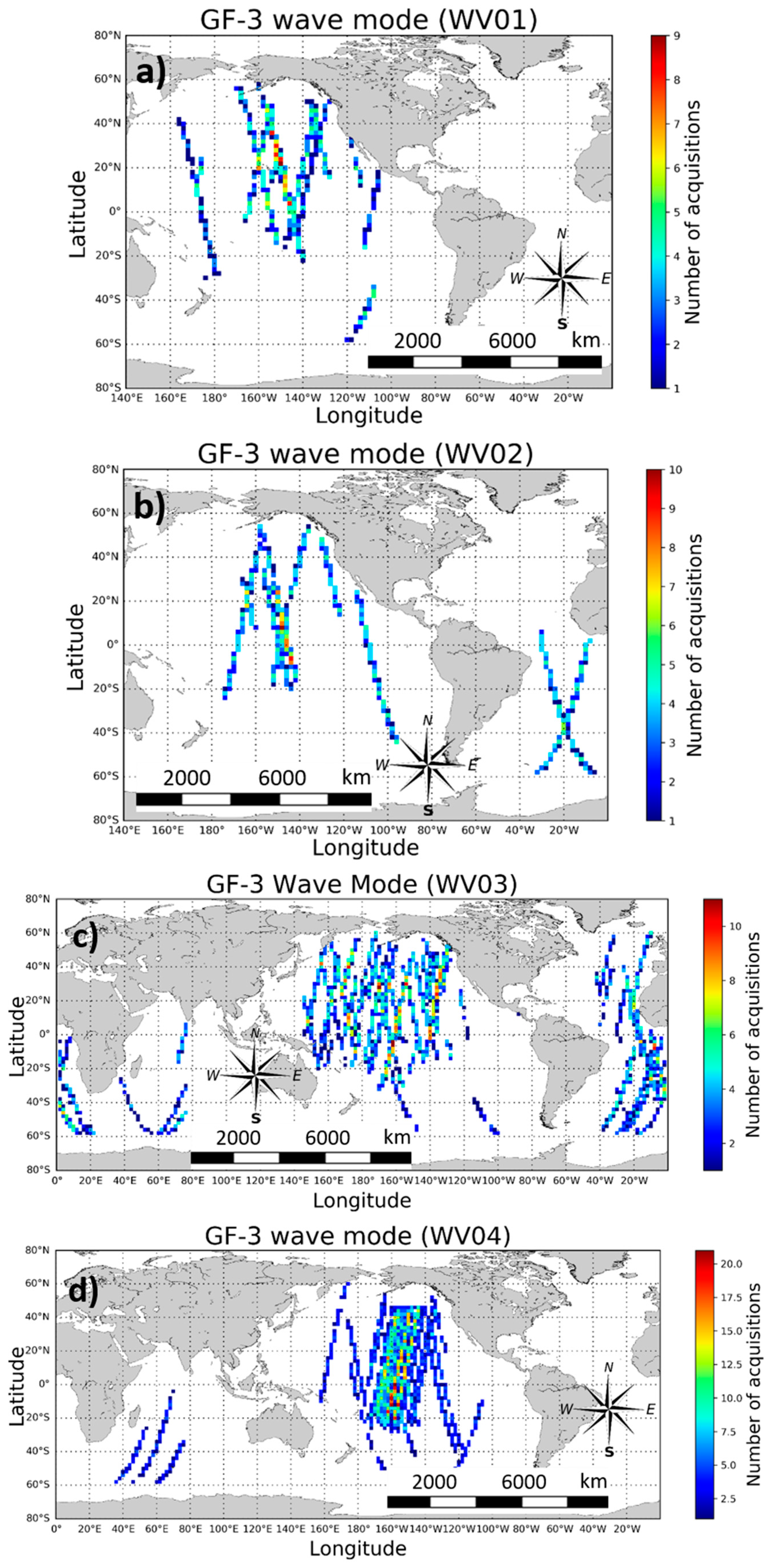
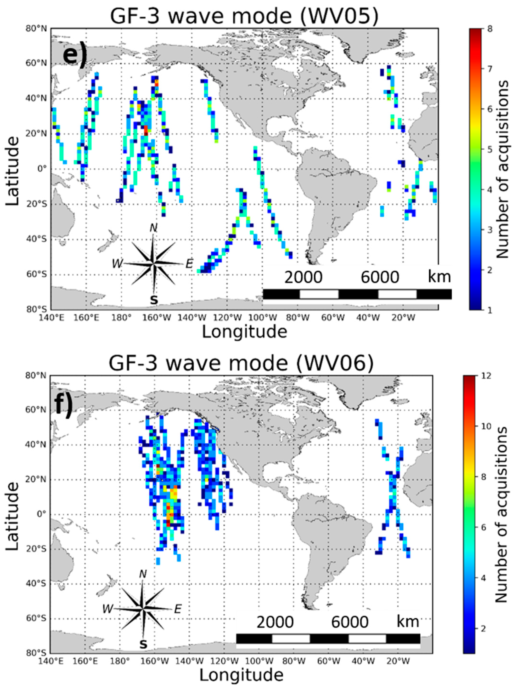
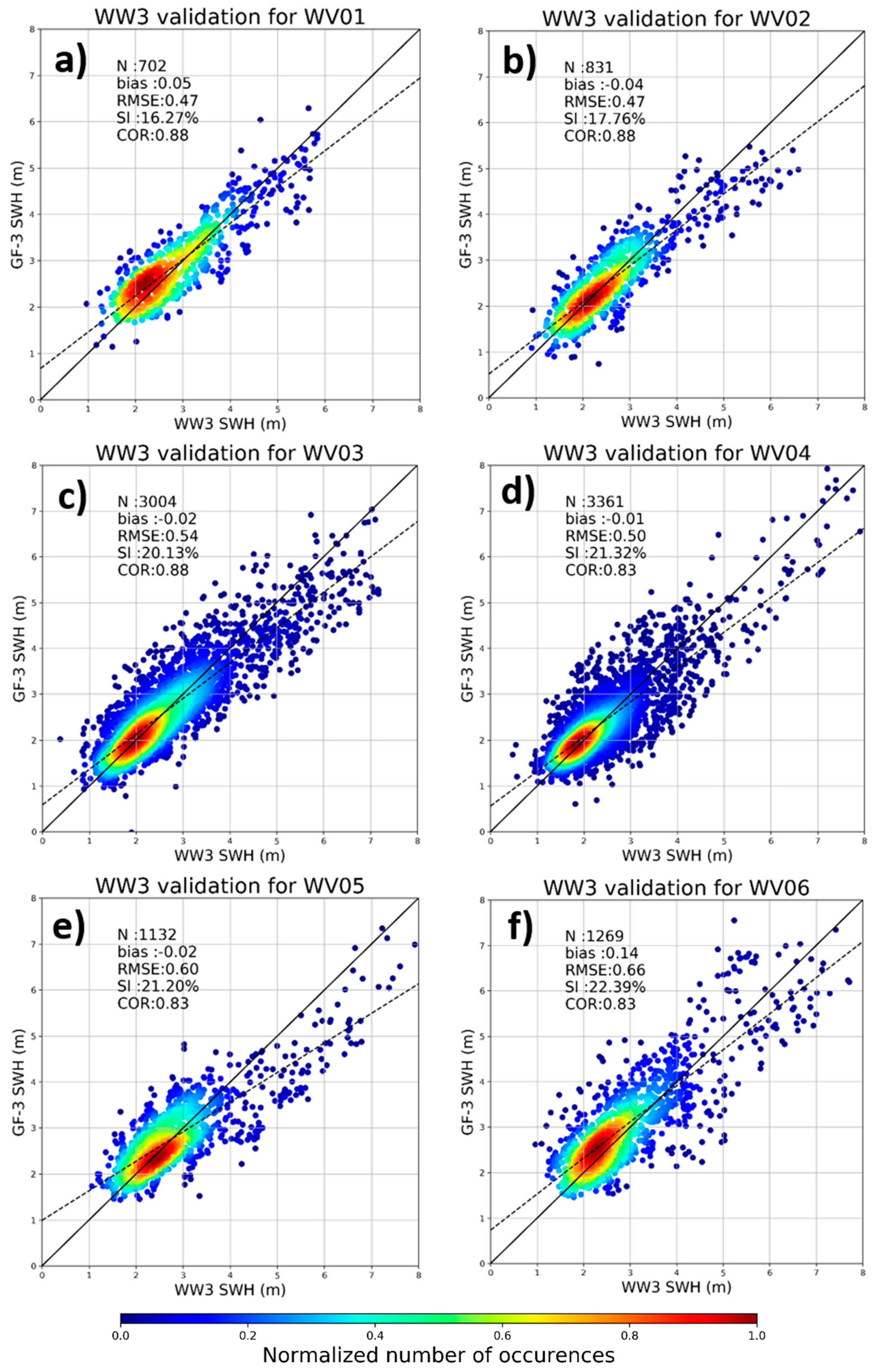
Incidence angle. WM imagettes from European SAR satellites are acquired at one or two specific incidence angles. In contrast, although a certain fixed incidence angle was adopted for a specific orbit, the incidence angle could be switched from 20 to 50° for WM on GF-3 for the period of ten months on which we focused. Hence, we categorized the GF-3 WM data into six groups with respect to incidence angle. Here, they are called incidence angle modes of WV01 for 21°–25°, WV02 for 28°–32°, WV03 for 33°–37°, WV04 for 38°–42°, WV05 for 42°–46°, and WV06 for 46°–50°, and details are listed in

Table 1. Information on GF-3 WM data for different incidence angle modes.

ID	Incidence Angle			Number of GF-3 WM Data
	Range	Mean	Standard Deviation	Total	Rejected	Tuning	Validation against WW3
WV01	21–25°	22.27°	1.03°	988	106	180	702
WV02	28–32°	29.92°	1.02°	1228	188	209	831
WV03	33–37°	35.80°	0.74°	4192	440	748	3004
WV04	38–42°	41.06°	0.97°	4742	545	836	3361
WV05	42–46°	44.08°	1.08°	1620	204	284	1132
WV06	46–50°	47.40°	1.20°	1758	170	319	1269

.

(3)

Geographic distribution. Traditional European SAR WM could monitor swells in the open ocean at a global scale e.g., [4]. However, currently, the GF-3 SAR payload can only work in WM for up to 50 min in one acquisition, owing to power limitations [31]. Thus, as shown in Figure 2, GF-3 WM measurements are not globally distributed for any of the 6 incidence angle modes in the period from January to October 2017.

In this study, only the GF-3 WM data exhibiting a pure ocean wave pattern (for a typical example, see Figure 1a) are used in the tuning and validation of the new empirical model. The following quality control procedures are applied here.

(1)

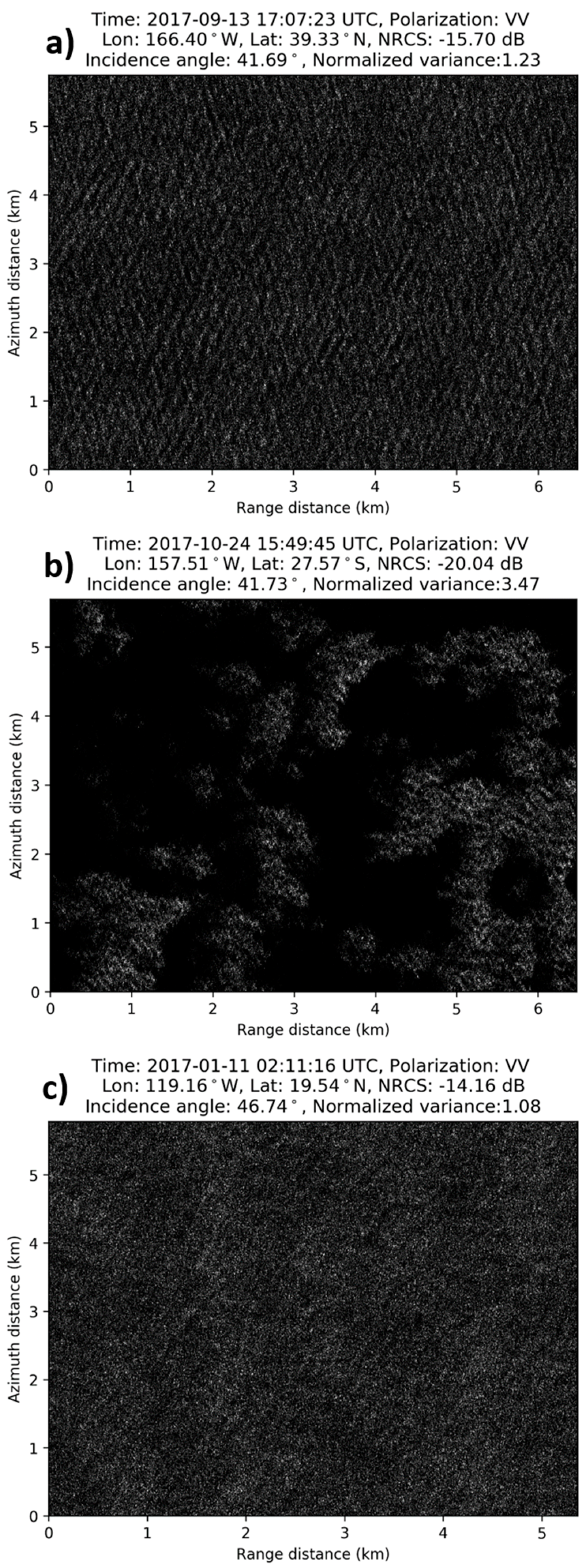
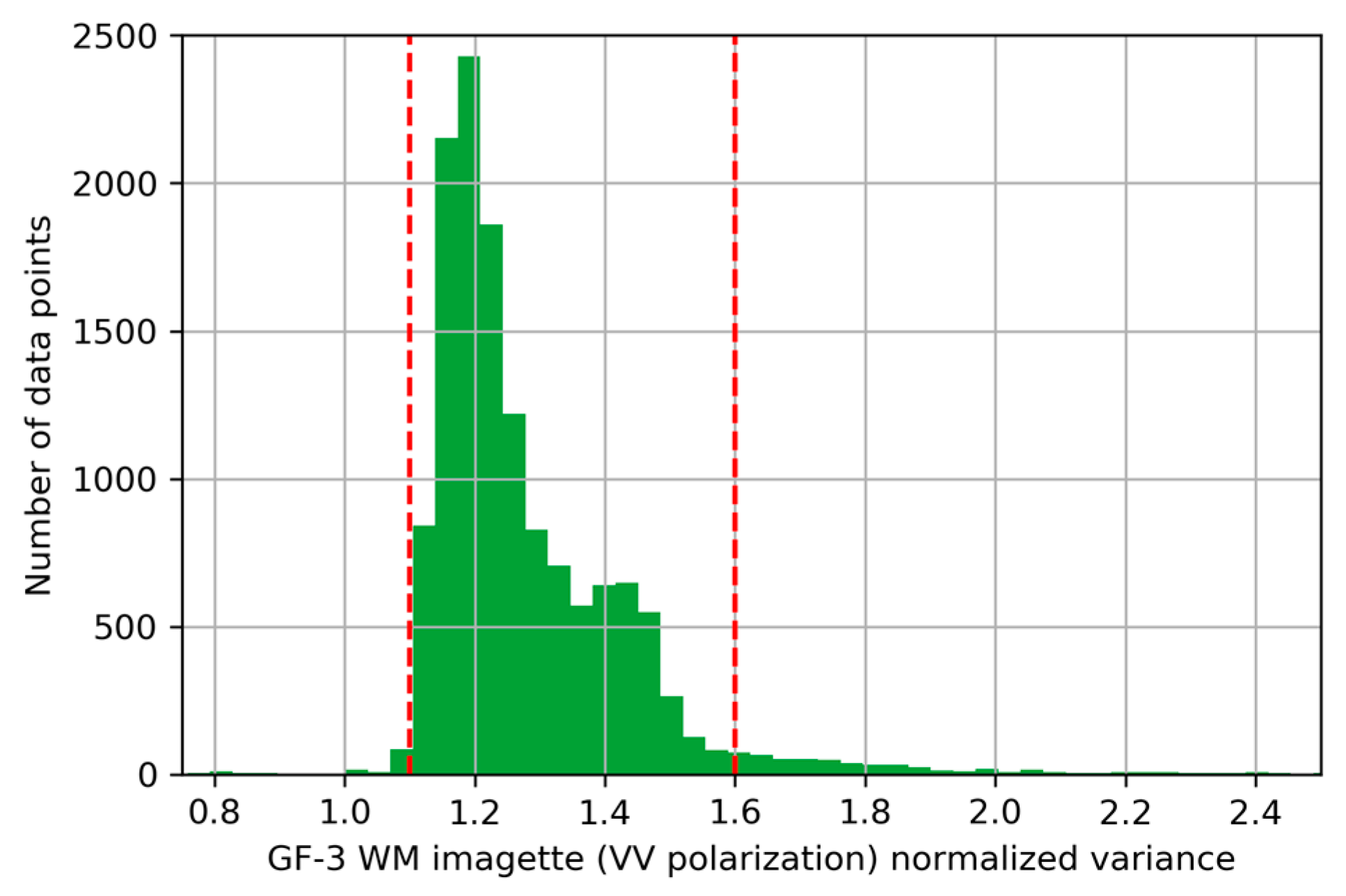
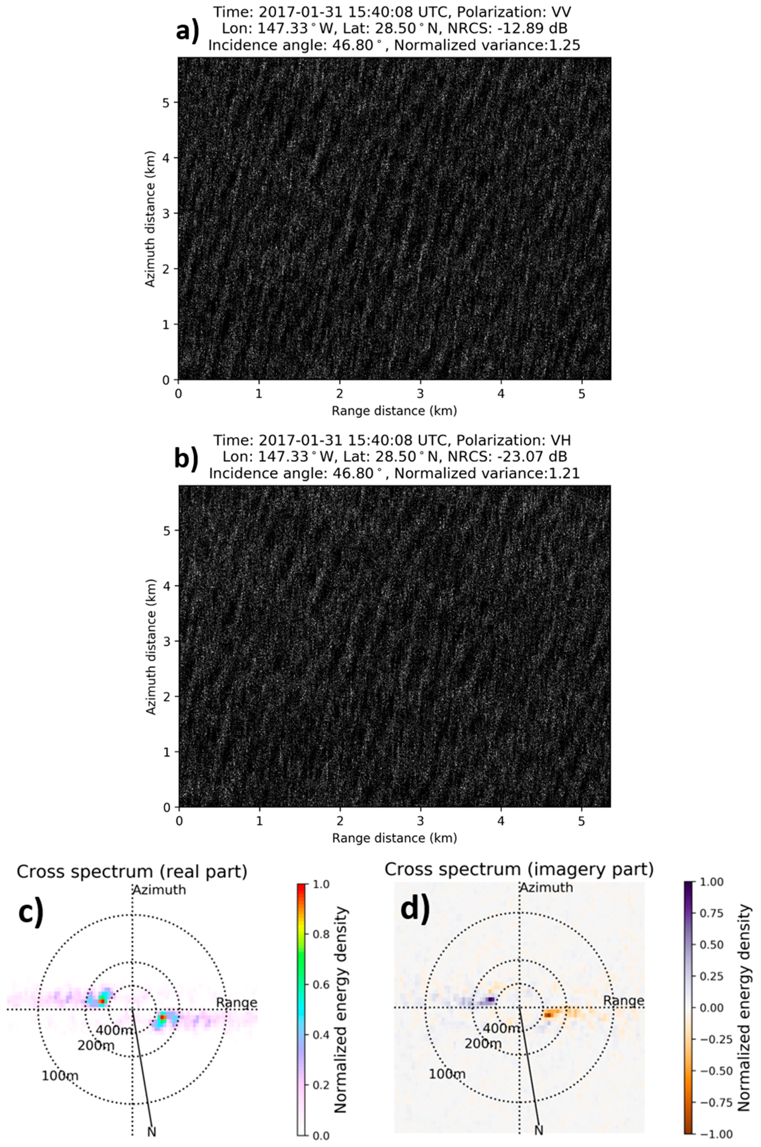
Homogeneity check. Here, the homogeneity quality control is performed using the parameter of normalized variance ($cvar\_vv$) computed from VV-polarized imagettes, defined as the imagette variance normalized with mean intensity:

$$cvar\_vv=\mathrm{var}(\frac{I-\langle I\rangle }{\langle I\rangle })$$

(1)

where $\langle I\rangle$ is the mean intensity of GF-3 WM data in VV polarization.

Theoretically, if the SAR image is contaminated with islands, slicks, current shears, atmospheric effects (i.e., Figure 1b) etc., the normalized variance takes values larger than expected from pure wave modulation only. Otherwise, for cases in which ocean wave modulation is weak and the majority of a detected signature is speckle noise, the normalized variance should be small and close to 1.0, as in the example shown in Figure 1c (although some kind of signature like atmospheric waves is visible in Figure 1c, there is no apparent ocean surface wave patterns). The normalized variance $cvar\_vv$, has thus been used as a parameter to reject non-wave SAR data in various studies e.g., [23,37,38,39,40,41].

Figure 3 shows the possibility distribution of normalized variance from GF-3 WM imagettes during the period from January to October 2017. For the histogram, the GF-3 WM normalized variance values are mostly distributed in the range of 1.1 to 1.6 (92% approximately). Hence, only GF-3 WM data with 1.1 < $cvar\_vv$ < 1.6 remain here for the development and validation of the SWH retrieval empirical algorithm.

(2)

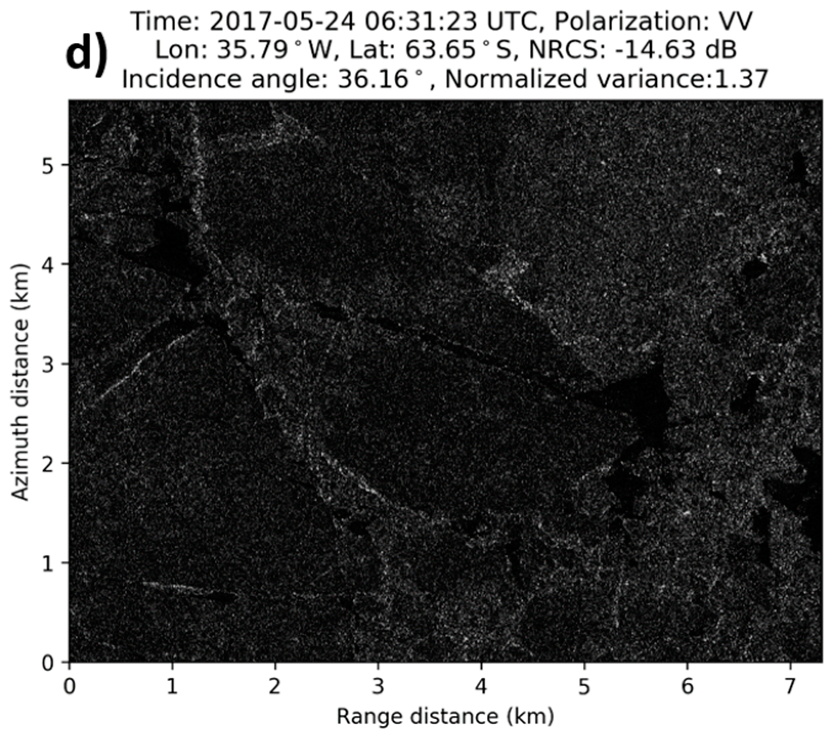
Ice rejection. For the SAR images acquired in the ice; for instance, Figure 1d presents homogeneous features but should be obviously excluded for our SWH retrieval. Because the $cvar\_vv$ check mentioned above fails to reject these cases ($cvar\_vv$ = 1.37 in Figure 1d), we further discarded the GF-3 WM acquisitions in high latitudes (>60°) to avoid sea ice near the polar regions.

Therefore, a total of 12,772 GF-3 WM data packets were selected out of 14,428 imagettes for the 10 months in 2017, resulting in a rejection rate of around 10%. Detailed numbers for each incidence angle mode (WV01 to WV06) can be found in Table 1.

Figure 2. Maps for GF-3 SAR WM acquisitions in data density for 2° × 2° bins for WV01 (a), WV02 (b), WV03 (c), WV04 (d), WV05 (e) and WV06 (f) from January to October 2017.

Figure 2. Maps for GF-3 SAR WM acquisitions in data density for 2° × 2° bins for WV01 (a), WV02 (b), WV03 (c), WV04 (d), WV05 (e) and WV06 (f) from January to October 2017.

Figure 3. Histogram of normalized variance computed from GF-3 WM imagettes (in VV polarization) for the period from January to October 2017.

Figure 3. Histogram of normalized variance computed from GF-3 WM imagettes (in VV polarization) for the period from January to October 2017.

2.2. Reference SWH Data

2.2.1. Wavewatch III Hindcast Data

The SWH hindcasts used here are from the database of IOWAGA (Integrated Ocean Waves for Geophysical and other Applications) project of IFREMER. The wave hindcasts were performed using the ocean wave model of WaveWatch III (WW3), with the parameterization of Rascle et al. [42] forced by the European Centre for Medium-range Weather Forecasts (ECMWF) winds. The outputs employed are a global grid of 0.5 × 0.5° × 3 h.

2.2.2. Altimeter SWH Data

Space-borne radar altimeters are another remotely sensed SWH data source, which are generally regarded to be more accurate than SAR derived SWH. To date, the existing altimeters are carried on the satellites of HY-2A, Jason-2/3, Cryosat-2, SARAL/Altika, and Sentinel-3. Using the temporal and spatial co-location criteria of 1 h and 100 km, only Ku-band HY-2A, Jason-2/3, and the Ka-band SARAL/Altika could be co-located with GF-3 WM images during our study period, with the location depicted in Figure 4. Following the calibrations proposed by Liu et al. [43]:

$$\mathrm{Jason}-2/3:SW{H}_{alt}^{*}=1.019\times SW{H}_{alt}-0.050$$

(2)

$$\mathrm{SARAL}:SW{H}_{alt}^{*}=0.997\times SW{H}_{alt}-0.056$$

(3)

$$\begin{gathered} \mathrm{HY}-\mathrm{2A}:SW{H}_{alt}^{*}= \\ \{\begin{array}{c}0.977\times SW{H}_{alt}+0.187SW{H}_{alt}\le 3.568\mathrm{m}\\ 0.013\times SW{H}_{alt}^2+1.083\times SW{H}_{alt}-0.359SW{H}_{alt}>3.568\mathrm{m}\end{array} \end{gathered}$$

(4)

where $SW{H}_{alt}^{*}$ and $SW{H}_{alt}$ are the calibrated and raw altimeter wave heights, SWH derived from different altimeters were corrected to be of consistent quality.

2.2.3. Buoy SWH Data

In situ SWH observations were collected from 27 National Data Buoy Center (NDBC) buoys whose locations are depicted in Figure 4 as red crosses. The hourly NDBC buoy records of SWH were co-located with GF-3 WM SAR data. In this study, the spatio-temporal criteria of 100 km and 0.5 h, yields 111 match-ups for the first 10 months of 2017.

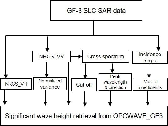
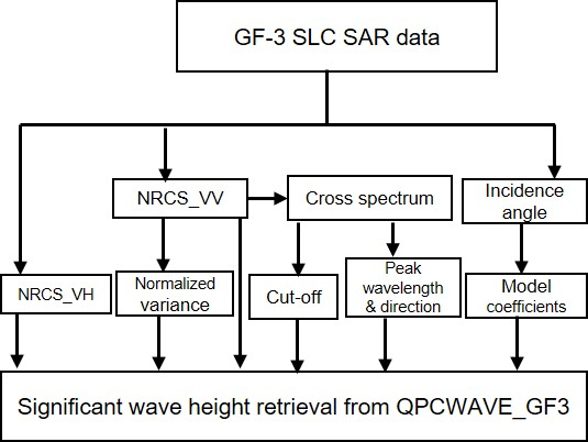
3. Development of Empirical Wave Retrieval Model: QPCWAVE_GF3

3.1. Radar Incidence Angle

Existing empirical SWH retrieval models for ERS-2 and Envisat/ASAR, i.e., CWAVE_ERS and CWAVE_ENV, are independent of incidence angle, due to their fixed angle of radar incidence in SAR WM configuration. In fact, the incidence angle is an important parameter that should be taken into consideration to build such empirical models [25,26,28]. With respect to Sentinel-1 A, whose WM configuration has two fixed incidence angles, CWAVE_S1A and CWAVE_Fnn [23] were developed for each of the two incidence beams respectively. Inspired by this, in order to deal with the radar incident dependency for GF-3 WM, as mentioned above, we subdivided the GF-3 WM images into six incidence modes (see Table 1 for details) and tuned our QPCWAVE_GF3 model for each incidence mode respectively.

3.2. Normalized Radar cross Section (NRCS)

SAR-observed NRCS ${\sigma }^0$ is directly related to the sea surface roughness of short surface waves, and is widely used for ocean wind retrievals i.e., [32,44,45]. Thus, NRCS can represent information on wind sea (short wave roughness) and co-polarized (VV) NRCS has been introduced into SAR empirical SWH algorithms [19,20,23]. Besides, C-band cross-polarization (VH or HV) has demonstrated good performance to extract high winds even in hurricanes when saturation was observed in co-polarization i.e., [46,47]. Thus, the SAR SWH empirical model could be expected to provide better performance on estimation of wind wave energy in high sea state by taking VH NRCS into consideration (see Section 5.1 for detailed discussion). Therefore, both co- and cross-polarized (VV/VH) NRCS measurements (denoted as ${\sigma }_{vv}^0$ and ${\sigma }_{vh}^0$ respectively) are included in our QPCWAVE_GF3 empirical model. In fact, SAR NRCS does not provide ocean wind speed directly, since NRCS observations depend also on incidence angle and relative wind direction. However, the NRCS, instead of SAR-derived wind speed, is chosen here as the input for our proposed empirical model. The reason is that the wind speed retrieval from co-polarized NRCS usually needs prior information of wind direction i.e., [32,48], and the wind speed estimation accuracy depends on the selection of different GMFs [16,17,18]. Thus, by including NRCS, we propose our SWH empirical model which could be implemented without using SAR-derived wind speeds.

3.3. Image Normalized Variance

The normalized variance which is used for the imagette inhomogeneity rejection (see Section 2.1) is also found to contain the longer wave information caused by the swell modulation [19,20,23]. Here, following the existing empirical SAR SWH models, normalized variance computed from VV polarized GF-3 WM imagettes, denoted as $cvar\_vv$ here, is selected as another input for the QPCWAVE_GF3 empirical model. See Equation (1) for the details on computation formula of $cvar\_vv$.

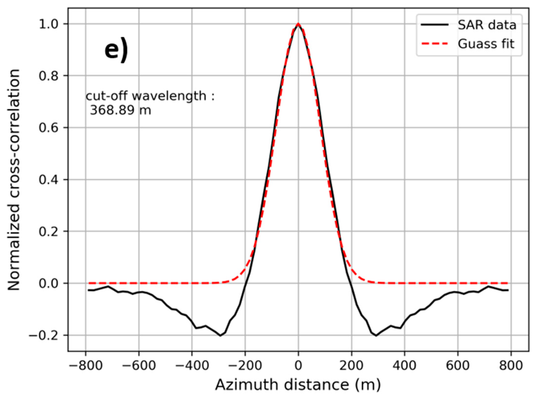
3.4. Azimuth Cut-Off, Peak Wavelength and Direction

According to the SAR-ocean imaging mechanism of velocity bunching, the relative motions between satellite and ocean surface scatters induce additional Doppler frequency shift, leading to strong cut-off in the SAR spectra in the azimuth direction [1,49]. This cut-off effect suppresses the spectral information provided by the SAR on short to moderate wavelength waves with components of propagation in the azimuth direction. However, it has been found that SAR azimuth cut-off could provide additional information on sea state [50], and is applied to some empirical SWH retrieval algorithms, e.g., [23,24,26,28].

Theoretically, the azimuth cut-off ${\lambda }_c$ can be expressed by

$${\lambda }_c=\mathsf{\pi }\beta \sqrt{{{\displaystyle \int }}^{\text{}}{\left|T_k^v\right|}^{2}S\left(f,\phi \right)dfd\phi }$$

(5)

where $\beta =\frac{R}{V}$ is the range ($R$) to velocity ($V$) ratio of the SAR platform, $f$ is the wave frequency, and $T_k^v$ represents the range velocity transfer function [1].

Based on the derivation and analysis from Wang et al. [24], the azimuth cut-off ${\lambda }_c$ could be theoretically related to the sea state in terms of $swh$ and mean wave period $T_0$ (related to wavelength ${\lambda }_p$ according to the wave dispersion law in deep water) by

$$\mathrm{swh}=\frac{2C}{{\pi }^2}\frac{{\lambda }_c}{\beta }{T}_0$$

(6)

with the dimensionless coefficient $C$ dependent on incidence angle $\theta$, and wave propagation direction $\phi$ (relative to radar look direction), expressed as

$$C=1/\sqrt{1-0.5si{n}^2\theta \left[1+\frac{\pi /\mathsf{{\rm B}}}{sinh\left(\pi /\mathsf{{\rm B}}\right)}cos\left(\pi -2\phi \right)\right]}$$

(7)

In addition, the directionality dependency of the $swh~{\lambda }_c/\beta$ relationship has been proven by simulations [26,28]. Therefore, it is evident that azimuth cut-off ${\lambda }_c$ is related to SWH with the dependency of peak wave direction $\phi$ and wavelength, as well as radar incidence angle. Thus, considering this complicated relationship, in contrast to the relative simple linear models e.g., [26,28], we include azimuth cut-off ${\lambda }_c$, peak wavelength ${\lambda }_p$, and direction $\phi$ into our QPCWAVE_GF3 model, and take their interactions into account as well.

3.5. Tuning of the Empirical Model QPCWAVE_GF3

From the analysis above, the empirical model is designed using six SAR-related parameters (VV and VH polarized NRCS ${\sigma }_{vv}^0$, ${\sigma }_{vh}^0$; normalized variance $cva{r}_{vv}$; azimuth cut-off ${\lambda }_c$; peak wavelength ${\lambda }_p,$ and direction $\phi$) and by considering their interactions. The proposed empirical model, called QPCWAVE_GF3 could be written as:

$$\begin{gathered} swh=A+B_1{\sigma }_{vh}^0+B_2\frac{{\lambda }_c}{\beta }+B_3{\lambda }_p+B_{4}cos\phi +B_5{\sigma }_{vv}^0+B_{6}cva{r}_{vv}+C_1\frac{{\lambda }_c}{\beta }{\lambda }_p+C_2\frac{{\lambda }_c}{\beta }cos\phi + \\ {C}_3{\sigma }_{vv}^{0}cos\phi +C_{4}cva{r}_{vv}cos\phi +C_{5}cva{r}_{vv}{\sigma }_{vv}^0 \end{gathered}$$

(8)

We randomly selected 20% of the GF-3 SAR-WW3 co-located data for tuning the model of QPCWAVE_GF3. The numbers of data pairs for each incidence mode are listed in Table 1. It is worth mentioning that the co-located GF-3 WM data with altimeters or buoys, and the GF-3 WM images discussed in Section 5.2.1 were not used in the tuning data, ensuring that the validation was independent. From the Ordinary Least Squares (OLS) regression, 12 coefficients of the empirical model are determined for each incidence mode from WV01 to WV06, as listed in

Table 2. Coefficients for QPCWAVE_GF3 model.

	WV01	WV02	WV03	WV04	WV05	WV06
$A$	−3.8082	−9.0969	1.5534	−19.5166	−10.4568	−9.4693
$B_1$	0.0015	0.1906	0.2429	0.1698	0.0988	0.4062
$B_2$	−0.6635	−0.8883	−0.7318	0.9653	−1.5123	−0.2300
$B_3$	0.0007	0.0017	−0.0024	0.0005	−0.0041	−0.0021
$B_4$	1.5233	5.9697	−0.1145	1.7617	1.9145	5.9112
$B_5$	−0.2459	−0.6458	−0.4577	−1.2828	−0.6397	−1.0020
$B_6$	4.2210	11.3454	3.6351	19.2854	14.5511	15.8545
$C_1$	0.0012	0.0010	0.0022	0.0002	0.0033	0.0014
$C_2$	2.0985	1.2722	1.0585	−0.3443	1.6726	0.8500
$C_3$	−0.0110	0.0370	0.1652	0.0616	0.0352	0.0476
$C_4$	−3.0297	−5.0699	0.8747	−0.3453	−3.5451	−5.5485
$C_5$	0.1713	0.3660	0.1349	0.9692	0.5105	0.5614

.

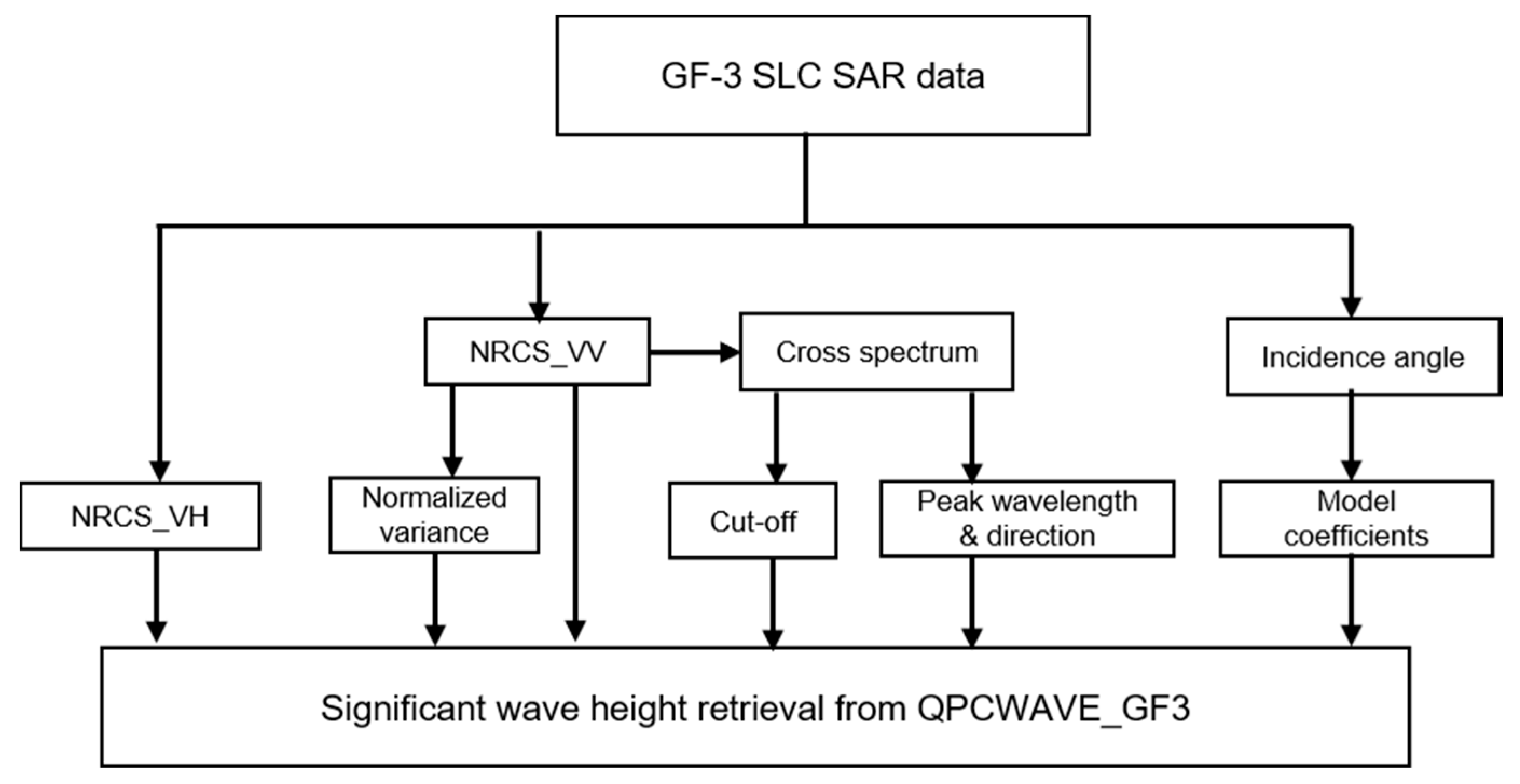
3.6. SWH Retrieval Scheme for GF-3 WM Data

The flowchart of the scheme for the SAR SWH empirical retrieval algorithm based on the developed QPCWAVE_GF3 model is shown in Figure 5, and the details can be summarized as follows. Here, we take the GF-3 wave mode acquisition over Northeast Pacific (147.33°W/28.50°N) at 15:35 Universal Time Coordinated (UTC) on 31 January 2017 as an example (Figure 6) to illustrate the QPCWAVE_GF3 SWH retrieval scheme.

(1) Radiometric calibration

The following formula is used for calibration of NRCS at VV and VH channels from Level-A GF-3 data:

$${\sigma }^0=10lo{g}_{10}\left[\mathrm{DN}\times {\left(\frac{qv}{32,767}\right)}^2\right]-K$$

(9)

where ${\sigma }^0$ is the NRCS united in dB, $\mathrm{DN}$ is the intensity calculated from GF-3 SAR Level-1A data, and $qv$ and $K$ are the external calibration constants stored in the product annotation file according to the polarizations. For instance, in the case shown in Figure 6, VV- and VH- polarized NRCS are −12.89 dB and −23.07 dB, respectively.

(2) SAR cross spectrum estimation

Three sub-looks are extracted from the entire integration time using the VV-polarized SLC WM imagette (Figure 6a) and are then used to compute the SAR cross-spectrum (e.g., Figure 6c,d for an example of the real and imaginary parts of the spectrum respectively) with reduced noise floor [51]. Furthermore, the SAR peak wavelength and direction corresponding to the maximum energy are computed directly from the 2-D cross spectrum.

(3) Cut-off estimation

The parameter of azimuth cut-off is derived from estimated cross-spectrum. As shown in Figure 6e, azimuth cut-off could be estimated by fitting a Gaussian function to the auto-covariance function of the cross-spectrum (real part), following the methodology proposed by Kerbaol et al. [49]. The Gaussian fit function is stated as,

$$exp{\left(-\frac{\pi x}{{\lambda }_c}\right)}^2$$

(10)

where $x$ denotes the spatial distance in the azimuth direction. The cut-off of 368.89 m was estimated for the case as depicted in Figure 6e, representing a strong azimuth cut-off effect consistent with the corresponding spectrum shown in Figure 6c.

(4) SWH empirical retrieval

Through the incidence angle, the 12 coefficients for the corresponding incidence mode of QPCWAVE_GF3 could be obtained. Thus, the SWH could be estimated from the computed parameters using Equation (8).

4. Algorithm Validation

To assess the accuracy of the proposed QPCWAVE_GF3 empirical model, the statistics of bias, Root Mean Square Error (RMSE), the Scatter Index (SI), and correlation coefficient (COR) were computed using the following expressions:

$$\mathrm{bias}=\frac{1}{N}{\displaystyle \sum }_{i=1}^N(x_i-y_i)$$

(11)

$$\mathrm{RMSE}=\sqrt{\frac{1}{N}{\displaystyle \sum }_{i=1}^N{(x_i-y_i)}^2}$$

(12)

$$\mathrm{SI}=\frac{1}{\langle x_i\rangle }\sqrt{\frac{1}{N}{\displaystyle \sum }_{i=1}^N{\left[\left(y_i-\langle y_i\rangle \right)-\left(x_i-\langle x_i\rangle \right)\right]}^2}\times 100\%$$

(13)

$$\mathrm{COR}=\frac{{{\displaystyle \sum }}_{i=1}^N\left(x_i-\langle x_i\rangle \right)-\left(y_i-\langle y_i\rangle \right)}{\sqrt{{{\displaystyle \sum }}_{i=1}^N{\left(x_i-\langle x_i\rangle \right)}^2{{\displaystyle \sum }}_{i=1}^N{\left(y_i-\langle y_i\rangle \right)}^2}}$$

(14)

where $x_i$ and $y_i$ represent the SWH from reference data and GF-3 retrievals using the QPCWAVE_GF3 model at the $i$th SAR WM acquisition, respectively; $N$ is the total number of data points in validation, and $\langle .\rangle$ denotes the average operator.

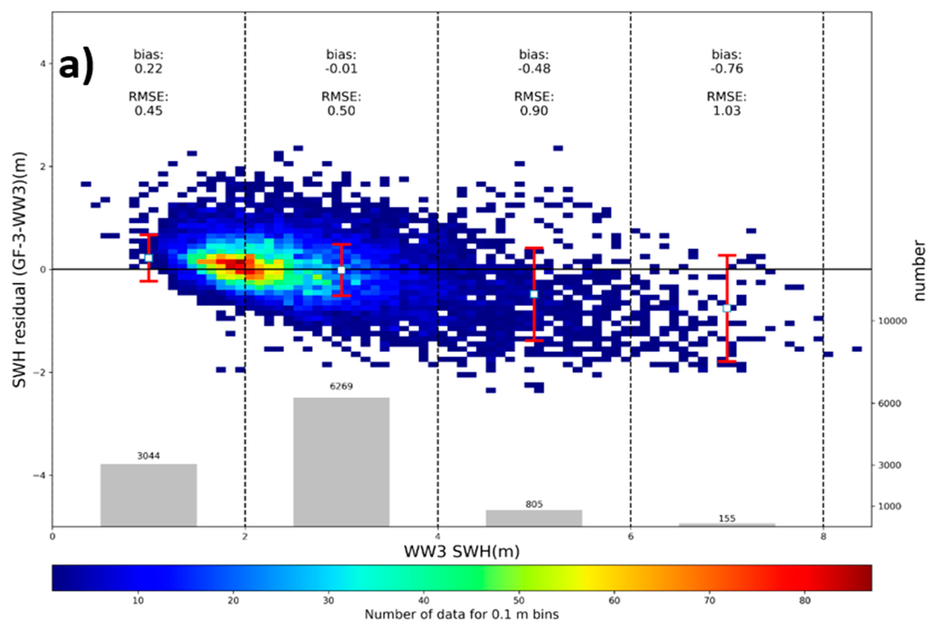
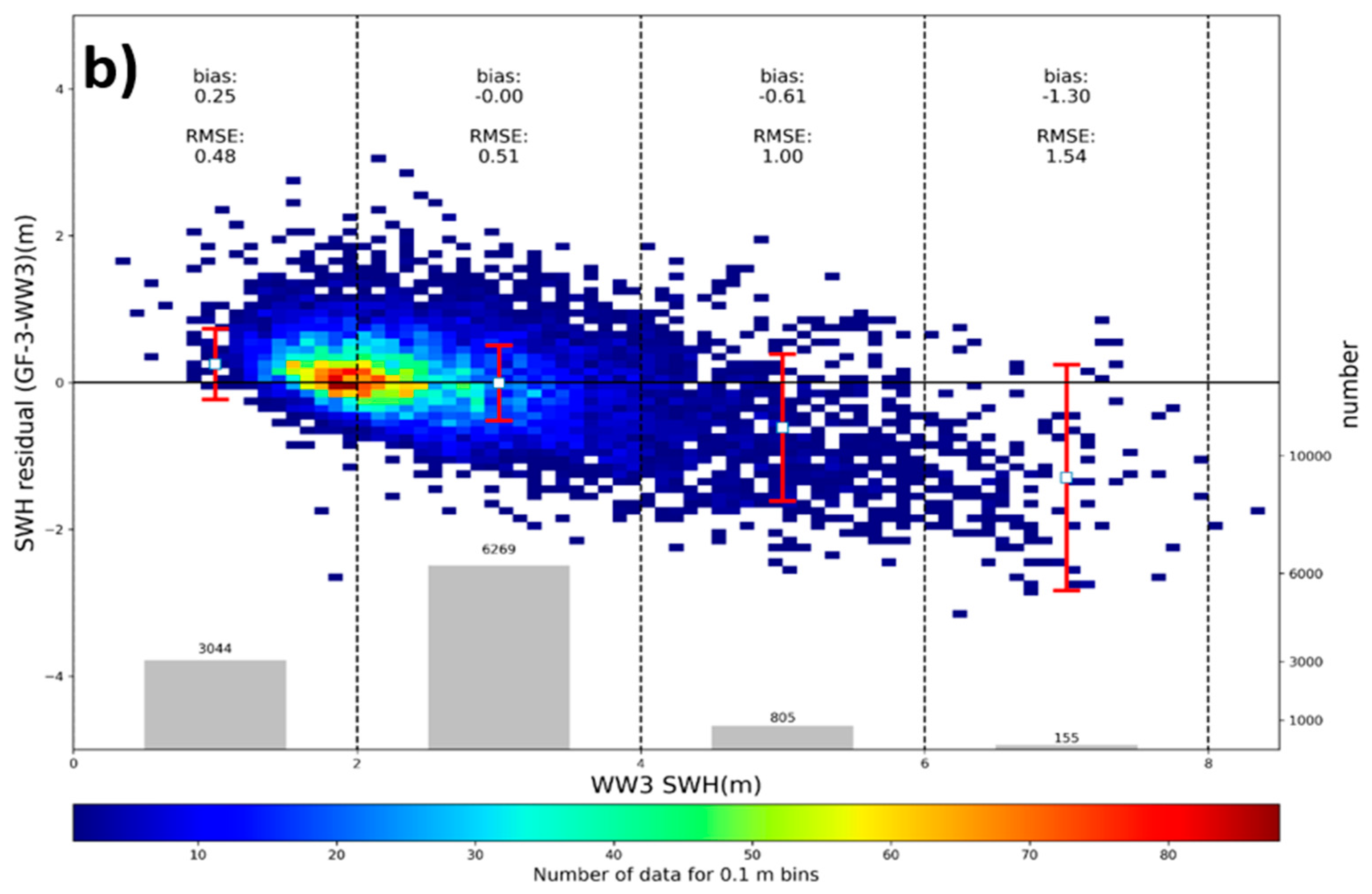
4.1. Comparison with Independent WW3 Hindcast

Figure 7 illustrates the validation results of QPCWAVE_GF3 empirical GF-3 SWH retrievals against independent WW3 wave model SWH hindcasts. In general, the validation result shows that the accuracy of the QPCWAVE_GF3 model differs for every incidence mode. The GF-3 SAR WM images at lower incidence angles (i.e., RMSE of 0.47 m and SI of 16.72% for WV01 with $\theta$ around 22.3°) perform better than those at larger incidence angles (i.e., RMSE of 0.66 m and SI of 22.39% for WV06 with $\theta$ around 47.4°). This may reveal the fact that lower incidence angles are more favorable for SAR ocean wave height retrieval. It is worth mentioning that the GF-3 WV01 ($\theta$ around 22.3°) and WV03 ($\theta$ around 35.8°), which are similar to the radar incidence configuration WV1 (23°) and WV2 (36°) of Sentinel-1A, could produce similar accuracy (WV01: RMSE of 0.47 m and SI of 16.72%; WV03: RMSE of 0.54 m and SI of 20.13%) using our proposed QPCWAVE_GF3 model, compared to those using CWAVE_S1A and CWAVE_Fnn [23].

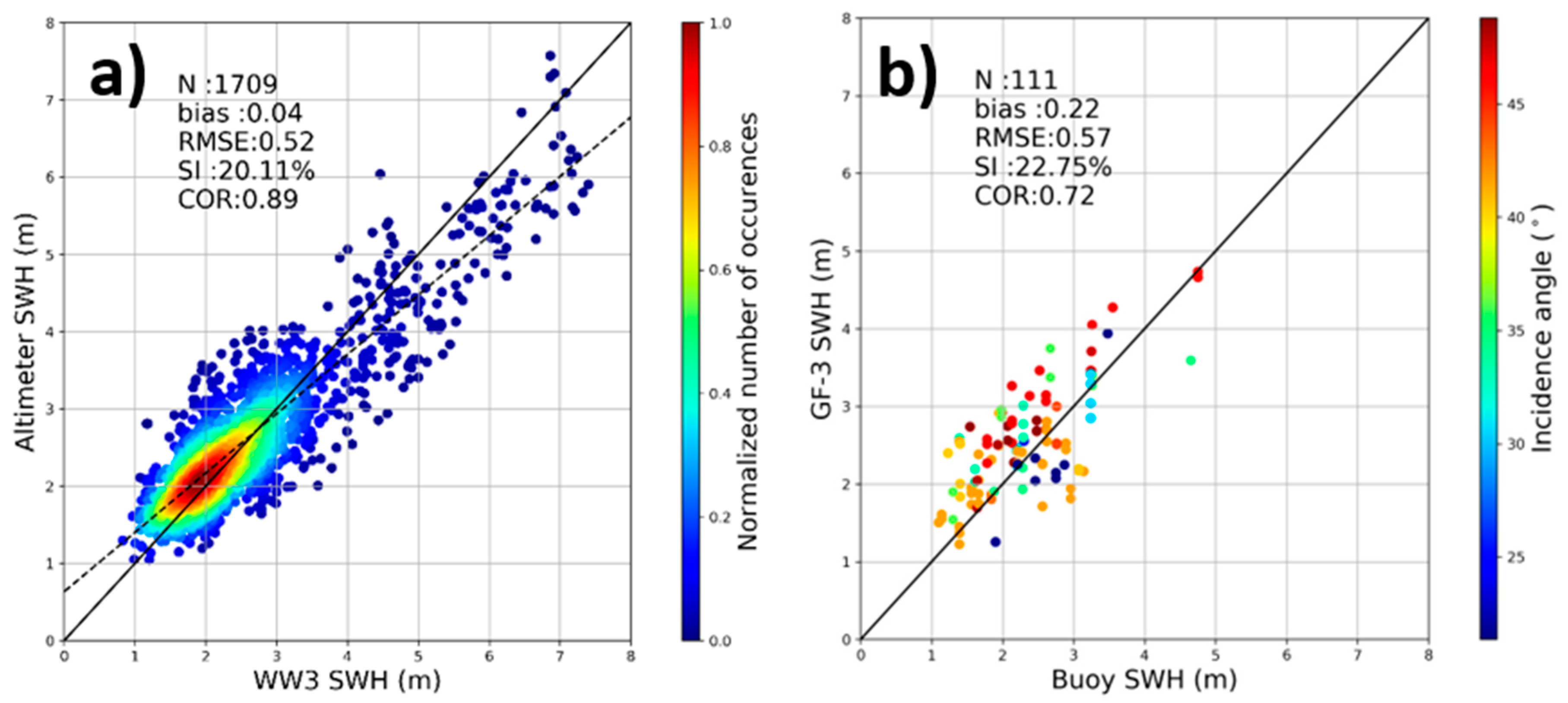
4.2. Comparison with Altimeters and Buoys

Figure 8a,b presents the comparisons of SWH derived from GF-3 SAR WM data using the QPCWAVE_GF3 model against the independent data set from altimeters and NDBC buoys, with 1709 and 111 co-located points, respectively. The validation against SWH derived from altimeters (HY-2A, Jason-2/3, SARAL) shows a good agreement with a RMSE of 0.52 m, SI of 20.11%, and correlation coefficient of 0.89. With respect to NDBC buoy measurements, the proposed QPCWAVE_GF3 empirical retrievals present accuracy of 0.57 m, 22.75%, and 0.72 in terms of RMSE, SI, and correlation coefficient, respectively. Both assessments through observation show similar results to the accuracy from the comparison with the WW3 model hindcast.

5. Discussions

5.1. Cross-Polarized NRCS Contribution to SWH Empirical Model

One of the features of the GF-3 WM data we focused on is the quad-polarization information provided by SAR data. Accordingly, the SWH retrieval algorithm QPCWAVE_GF3 proposed here includes the cross-polarized NRCS, which have been not taken into account for the empirical models dedicated to single polarization SAR data i.e., [19,20,23], or even Radarsat-2 SAR images with quad-polarization [28]. Therefore, it is interesting to discuss the contribution of cross-polarized NRCS to our proposed empirical SWH retrieval algorithm.

In contrast to the QPCWAVE_GF3 model represented by Equation (8), another empirical model excluding cross-polarized NRCS could be built as

$$\begin{gathered} swh=a+b_1\frac{{\lambda }_c}{\beta }+b_2{\lambda }_p+b_{3}cos\phi +b_4{\sigma }_{vv}^0+b_{5}cva{r}_{vv}+c_1\frac{{\lambda }_c}{\beta }{\lambda }_p+c_2\frac{{\lambda }_c}{\beta }cos\phi + \\ {c}_3{\sigma }_{vv}^{0}cos\phi +c_{4}cva{r}_{vv}cos\phi +c_{5}cva{r}_{vv}{\sigma }_{vv}^0 \end{gathered}$$

(15)

and tuned using the same WW3 modelling dataset as QPCWAVE_GF3, with 11 coefficients for the 6 incidence modes of GF-3 WM (not shown).

Figure 9a,b show the comparisons of GF-3 SWH retrievals against independent WW3 modelling SWH for all GF-3 WM incidence angles, by using empirical model of QPCWAVE_GF3 (Equation (8)) and the one excluding cross-polarized NRCS (Equation (15)), respectively. In general, the validation results indicate that the accuracy of the empirical model is degraded by rejecting cross-polarized NRCS in terms of RMSE (from 0.54 m to 0.59 m), SI (from 20.64 to 22.32%), and COR (from 0.86 to 0.83).

From Figure 9, one can obviously see the much larger inconsistency between GF-3 SWH retrievals from the empirical model without cross-polarized NRCS in high sea states. In order to investigate this, we analyzed the SWH residual of the GF-3 retrieval using the empirical model with and without cross-polarized NRCS with respect to the WW3 SWH, as shown in Figure 10. There is no apparent discrepancy regarding the SWH residual when including and excluding cross-polarized NRCS. However, in the high sea state (SWH above 6 m), the proposed QPCWAVE_GF3 model could be improved by reducing RMSE from 1.54 m to 1.03 m and bias from −1.30 m to −0.76 m with the help of cross-polarized NRCS.

5.2. Case Studies

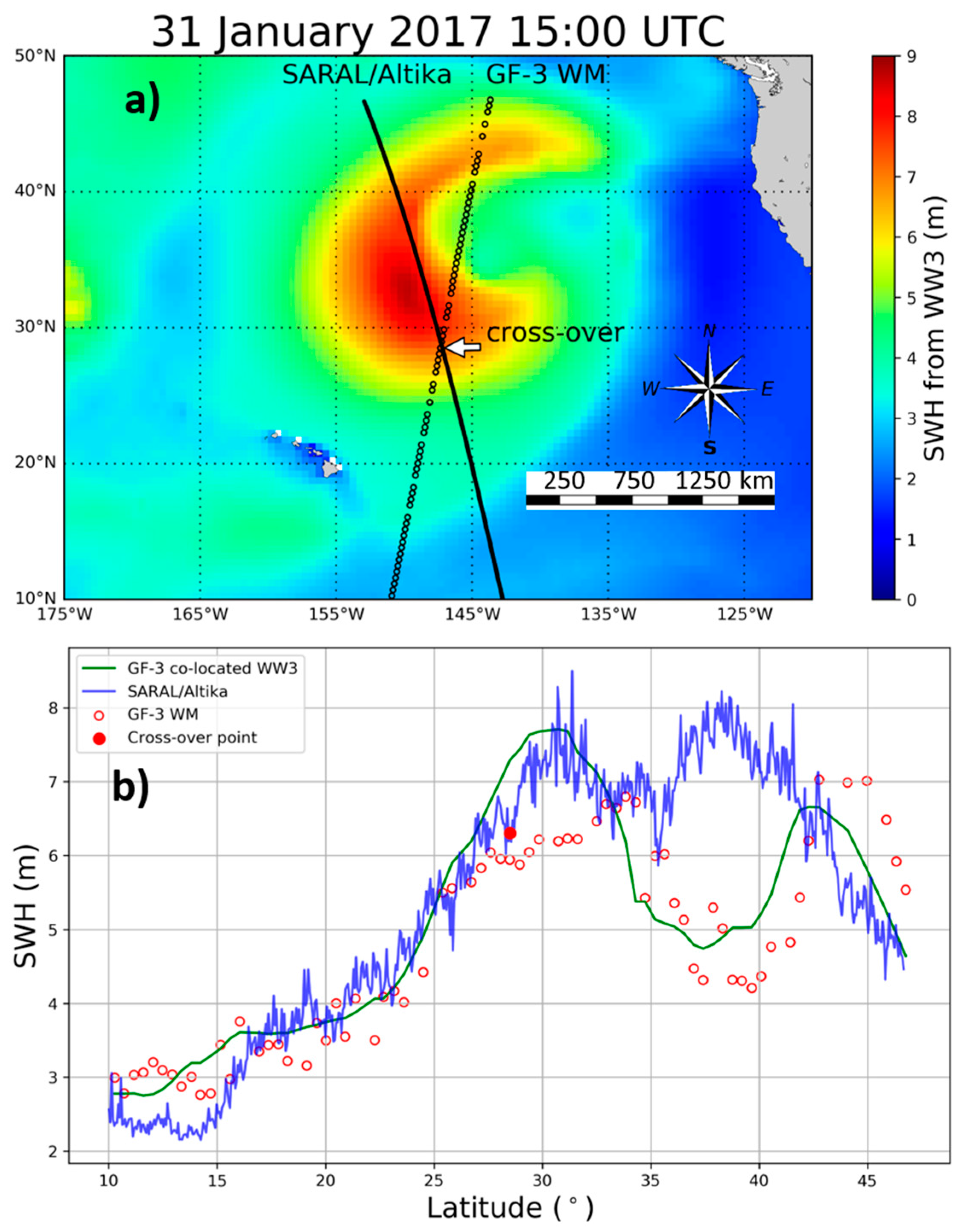
5.2.1. Case of 31 January 2017 from GF-3 WM Data

On 31 January 2017, a storm with big waves occurred northeast of Hawaii, as reported by WW3 modelling as shown in Figure 11a (colors denote the SWH hindcast at 15:00 UTC). This event was captured by GF-3 in WM from 15:35:00 to 15:45:14 UTC on the same date represented by the red circles in Figure 11a. Fortunately, the SARAL/Altika altimeter also passed over this storm from 15:26:20 to 15:36:42 UTC, 31 January 2017 as depicted by the black line in Figure 11a. Moreover, the GF-3 and SARAL were cross co-located at 15:40 UTC, and the cross-over point (147.33°W/28.50°N) is annotated in Figure 11a. This match-up GF-3 WM observation (see Figure 6) has been presented by demonstrating the retrieval scheme in Section 3.6.

Along the transect of GF-3 WM, the WW3 hindcast and SWH retrievals using the proposed QPCWAVE model are shown in Figure 11b as the red circles and green line, respectively. Agreement can be seen regarding the WW3 modelled SWH ranging 3–4 m, mainly located between 10°N and 25°N. However, the GF-3 SWH retrievals from QPCWAVE are underestimated against the WW3 hindcast for SWH above 4 m, especially between 25°N and 35°N (WW3 SWH > 6 m). Moreover, between 25°N and 30°N, where the SAR and altimeter passed nearby in space, the QPCWAVE estimations are closer to the SARAL/Altika-derived SWH (i.e., 5.94 m vs. 6.30 m from GF-3 and SARAL, respectively, for the cross-over point) than WW3 modelling, although underestimation could be found as well. This discrimination is in line with the statistical comparisons shown in Figure 7, Figure 8 and Figure 9, implying the limitation of our proposed QPCWAVE empirical model in very high sea states (>6 m).

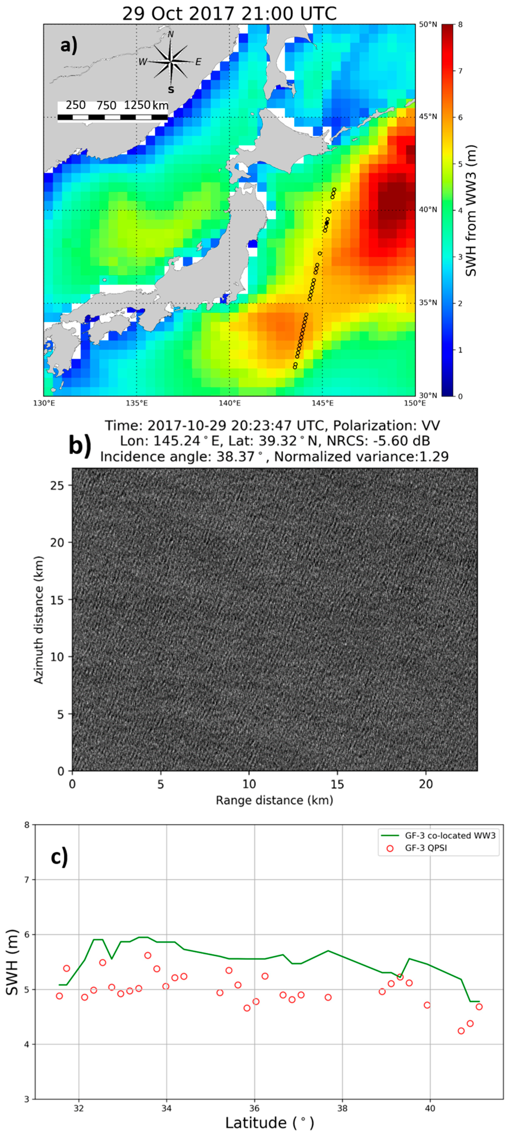
5.2.2. Case of 29 October 2017 from GF-3 QPSI Data

High sea states (above 5 m hindcast by WW3 at 21:00 UTC as shown in Figure 12a) caused by Tropical Storm Saola predominated in the east of Japan on 29 October 2017. A successive descending pass of GF-3 SAR images were acquired from 20:23:17 to 20:25:58 UTC on 29 October as represented by circles in Figure 12a. There were no altimeters flying over this area during this time.

These GF-3 SAR images were acquired in the working mode of QPSI rather than WM. The GF-3 QPSI mode has a similar configuration to WM, but with the larger image coverage of 25 × 25 km (see Figure 12b) and is mainly dedicated to land and coastal areas [31]. Thus, the proposed QPCWAVE_GF3 model was applied to these QPSI images (the radar incidence angle of 38.37° is equivalent to WV04 for this case).

Figure 12c shows the comparison of WW3 hindcast and GF-3 QPSI SAR SWH estimated using the QPCWAVE_GF3 empirical model along the pass of GF-3. One can see quite good agreement, with a mean bias of 0.54 m, considering the high waves (average of 5.64 m from WW3 along this transect). Furthermore, although only GF-3 WM data were used for development of our proposed empirical model, the case introduced here could demonstrate the capability of the QPCWAVE_GF3 model to estimate from SAR data rather than GF-3 WM.

6. Conclusions

In this paper, we proposed a new approach of a direct retrieval of ocean wave SWH from GF-3 SAR WM data without transformation into wave spectra. The empirical model, called QPCWAVE_GF3, uses parameters from the quad-polarized SAR image and cross-spectrum to estimate the SWH. These inputs include VV- and VH-polarized NRCS, image normalized variance, azimuth cut-off wavelength, and peak wavelength and direction.

Using a co-located dataset of WW3 and GF-3 WM with a total of 2579 data points, the QPCWAVE_GF3 model is trained for six different radar incidence angle modes of GF-3 WM, and empirical coefficients have been determined.

The accuracy assessment of the SWH from GF-3 was carried out through a comparison with independent WW3 modelling hindcasts, and observations from altimeters and buoys for the period of ten months in 2017. The validations show RMSEs from 0.5 m to 0.6 m, and SI around 20% for six different incidence angle modes. Due to the quad-polarization capability of GF-3 WM data, our empirical model QPCWAVE_GF3 performs better in the high sea state by including cross-polarized NRCS. Besides, two cases of storm-induced high waves seen by GF-3 WM and QPSI mode are presented. The case study results indicate that our proposed model could be employed to estimate SWH from other similar quad-polarized SAR images, although it is tuned based on GF-3 WM data.

Future work will be dedicated to using more data, especially those in high sea states, to tune our empirical model, so that its accuracy can be improved in extreme wave conditions. In addition, the possibility of estimating SWH from C-band quad-polarized SAR images, such as Radarsat-2 data, could be investigated.

References

1. Hasselmann, K.; Hasselmann, S. On the nonlinear mapping of an ocean wave spectrum into a synthetic aperture radar image spectrum. J. Geophys. Res. 1991, 96, 10713–10729. [Google Scholar] [CrossRef]
2. Pugliese Carratelli, E.; Dentale, F.; Reale, F. Numerical PSEUDO-Random Simulation of SAR Sea and Wind Response. In Advances in SAR Oceanography from Envisat and ERS Missions, Proceedings of the SEASAR 2006 (ESA SP-613), Frascati (RM), Italy, 23–26 January 2006; Lacoste, H., Ed.; ESA Publications Division (ESTEC): Noordwijk, The Netherlands, 2006. [Google Scholar]
3. Pugliese Carratelli, E.; Dentale, F.; Reale, F. Reconstruction of SAR Wave Image Effects through Pseudo Random Simulation. In Proceedings of the Envisat Symposium 2007 (ESA SP-636), Montreux, Switzerland, 23–27 April 2007; Lacoste, H., Ouwehand, L., Eds.; ESA Communication Production Office (ESTEC): Noordwijk, The Netherlands, 2007. [Google Scholar]
4. Hasselmann, K.; Chapron, B.; Aouf, L.; Ardhuin, F.; Collard, F.; Engen, G.; Hasselmann, S.; Heimbach, P.; Janssen, P.A.E.M.; Johnsen, H.; et al. The ERS SAR wave mode: A breakthrough in global ocean wave observations. In ERS Missions: 20 Years of Observing Earth, 1st ed.; Fletcher, K., Ed.; European Space Agency: Noordwijk, The Netherlands, 2013; pp. 165–198. [Google Scholar]
5. Collard, F.; Ardhuin, F.; Chapron, B. Monitoring and analysis of ocean swell fields from space: New methods for routine observations. J. Geophys. Res. 2009, 114. [Google Scholar] [CrossRef]
6. Ardhuin, F.; Chapron, B.; Collard, F. Observation of swell dissipation across oceans. Geophys. Res. Lett. 2009, 36, 1–5. [Google Scholar] [CrossRef]
7. Ardhuin, F.; Collard, F.; Chapron, B.; Girard-Ardhuin, F.; Guitton, G.; Mouche, A.; Stopa, J.E. Estimates of ocean wave heights and attenuation in sea ice using the SAR wave mode on Sentinel-1A. Geophys. Res. Lett. 2015, 42, 2317–2325. [Google Scholar] [CrossRef]
8. Aouf, L.; Lefevre, J.M.; Hauser, D.; Chapron, B. On the combined assimilation of RA-2 and ASAR wave data for the improvement of wave forecasting. In Proceedings of the 2006 15 Years of Radar Altimetry Symposium, Venice, Italy, 13–18 March 2006. [Google Scholar]
9. Li, X.M. A new insight from space into swell propagation and crossing in the global oceans. Geophys. Res. Lett. 2016, 43, 5202–5209. [Google Scholar] [CrossRef]
10. Wang, H.; Mouche, A.; Husson, R.; Chapron, B.; Jiang, H. A global distribution of crossing swell from Envisat ASAR Wave Mode data based on swell propagation. In Proceedings of the Geoscience and Remote Sensing Symposium (IGARSS), 2016 IEEE International, Beijing, China, 10–15 July 2016. [Google Scholar]
11. Hasselmann, S.; Bruning, C.; Hasselmann, K. An improved algorithm for the retrieval of ocean wave spectra from synthetic aperture radar image spectra. J. Geophys. Res. 1996, 101, 6615–6629. [Google Scholar] [CrossRef]
12. Schulz-Stellenfleth, J.; Lehner, S.; Hoja, D. A parametric scheme for the retrieval of two-dimensional ocean wave spectra from synthetic aperture radar look cross spectra. J. Geophys. Res. 2005, 110, 297–314. [Google Scholar] [CrossRef]
13. Sun, J.; Kawamura, H. Retrieval of surface wave parameters from SAR images and their validation in the coastal seas around Japan. J. Oceanogr. 2009, 65, 567–577. [Google Scholar] [CrossRef]
14. Zhang, B.; Li, X.F.; Perrie, W.; He, Y.J. Synergistic measurements of ocean winds and waves from SAR. J. Geophys. Res. 2015, 120, 6164–6184. [Google Scholar] [CrossRef]
15. Chapron, B.; Johnsen, H.; Garello, R. Wave and wind retrieval from SAR images of the ocean. Ann. Telecommun. 2001, 56, 682–699. [Google Scholar]
16. Stoffelen, A.; Anderson, D. Scatterometer data interpretation: Estimation and validation of the transfer function CMOD4. J. Geophys. Res. 1997, 102, 5767–5780. [Google Scholar] [CrossRef]
17. Hersbach, H. Comparison of C-band scatterometer CMOD5.N equivalent neutral winds with ECMWF. J. Atmos. Ocean. Tech. 2010, 27, 721–736. [Google Scholar] [CrossRef]
18. Stoffelen, A.; Verspeek, J.A.; Vogelzang, J.; Verhoef, A. The CMOD7 geophysical model function for ASCAT and ERS wind retrievals. IEEE J. Sel. Top. Appl. Earth. Obs. Remote Sens. 2017, 10, 2123–2134. [Google Scholar] [CrossRef]
19. Schulz-Stellenfleth, J.; Konig, T.; Lehner, S. An empirical approach for the retrieval of integral ocean wave parameters from synthetic aperture radar data. J. Geophys. Res. 2007, 112, 1–14. [Google Scholar] [CrossRef]
20. Li, X.M.; Lehner, S.; Bruns, T. Ocean wave integral parameter measurements using Envisat ASAR wave mode data. IEEE Trans. Geosci. Remote Sens. 2011, 49, 155–174. [Google Scholar] [CrossRef] [Green Version]
21. Bruck, M. Sea state measurements using the XWAVE algorithm. Int. J. Remote Sens. 2015, 36, 3890–3912. [Google Scholar] [CrossRef]
22. Pleskachevsky, A.L.; Rosenthal, W.; Lehner, S. Meteo-Marine parameters for highly variable environment in coastal regions from satellite radar images. ISPRS J. Photogramm. Remote Sens. 2016, 119, 464–484. [Google Scholar] [CrossRef]
23. Stopa, J.E.; Mouche, A.A. Significant wave heights from Sentinel-1 SAR: Validation and applications. J. Geophys. Res. 2017, 122, 1827–1848. [Google Scholar] [CrossRef]
24. Wang, H.; Zhu, J.; Yang, J.S. A semi-empirical algorithm for SAR wave height retrieval and its validation using Envisat ASAR wave mode data. Acta Oceanol. Sin. 2012, 31, 59–66. [Google Scholar]
25. Grieco, G.; Lin, W.; Migliaccio, M.; Nirchio, F.; Portabella, M. Dependency of the Sentinel-1 azimuth wavelength cut-off on significant wave height and wind speed. Int. J. Remote Sens. 2016, 37, 5086–5104. [Google Scholar] [CrossRef]
26. Shao, W.Z.; Zhang, Z.; Li, X.F.; Li, H. Ocean wave parameters retrieval from Sentinel-1 SAR imagery. Remote Sens. 2016, 8, 707. [Google Scholar] [CrossRef]
27. Romeiser, R.; Graber, H.C.; Caruso, M.J.; Jensen, R.E.; Walker, D.T.; Cox, A.T. A new approach to ocean wave parameter estimates from C-band ScanSAR images. IEEE Trans. Geosci. Remote Sens. 2015, 53, 1320–1345. [Google Scholar] [CrossRef]
28. Ren, L.; Yang, J.S.; Zheng, G.; Wang, J. Significant wave height estimation using azimuth cutoff of C-band RADARSAT-2 single-polarization SAR images. Acta Oceanol. Sin. 2015, 12, 1–9. [Google Scholar] [CrossRef]
29. Shao, W.Z.; Wang, J.; Li, X.F.; Sun, J. An Empirical Algorithm for Wave Retrieval from Co-Polarization X-Band SAR Imagery. Remote Sens. 2017, 9, 711. [Google Scholar] [CrossRef]
30. Zhang, Q. System Design and Key Technologies of the GF-3 Satellite (in Chinese). Acta Geod. Cartogr. Sin. 2017, 46, 269–277. [Google Scholar] [CrossRef]
31. Sun, J.; Yu, W.; Deng, Y. The SAR payload design and performance for the GF-3 mission. Sensors 2017, 17, 2419. [Google Scholar] [CrossRef] [PubMed]
32. Wang, H.; Yang, J.S.; Mouche, A.; Shao, W.Z.; Zhu, J.H.; Ren, L.; Xie, C.H. GF-3 SAR ocean wind retrieval: The first view and preliminary assessment. Remote Sens. 2017, 9, 694. [Google Scholar] [CrossRef]
33. Shao, W.Z.; Sheng, Y.X.; Sun, J. Preliminary assessment of wind and wave retrieval from Chinese Gaofen-3 SAR imagery. Sensors 2017, 17, 1705. [Google Scholar] [CrossRef] [PubMed]
34. Yang, J.S.; Ren, L.; Wang, J. The first quantitative remote sensing of ocean surface waves by Chinese GF-3 SAR satellite. Oceanol. Limnol. Sin. 2017, 48, 207–209. [Google Scholar] [CrossRef]
35. Yang, J.S.; Ren, L.; Wang, J.; Zheng, G.; Li, X. Preliminary retrieval of ocean winds and waves from Chinese newly launched spaceborne microwave sensors. In Proceedings of the Geoscience and Remote Sensing Symposium (IGARSS), 2017 IEEE International, Forth Worth, TX, USA, 23–28 July 2017. [Google Scholar]
36. Ren, L.; Yang, J.S.; Mouche, A.; Wang, H.; Wang, J.; Zheng, G.; Zhang, H.G. Preliminary Analysis of Chinese GF-3 SAR Quad-Polarization Measurements to Extract Winds in Each Polarization. Remote Sens. 2017, 9, 1215. [Google Scholar] [CrossRef]
37. Wang, H.; Zhu, J.; Yang, J. Error Analysis on ESA’s Envisat ASAR Wave Mode Significant Wave Height Retrievals Using Triple Collocation Model. Remote Sens. 2014, 6, 12217–12233. [Google Scholar] [CrossRef]
38. Stopa, J.E.; Ardhuin, F.; Husson, R.; Jiang, H.; Chapron, B.; Collard, F. Swell dissipation from 10 years of Envisat advanced synthetic aperture radar in wave mode. Geophys. Res. Lett. 2016, 43, 3423–3430. [Google Scholar] [CrossRef]
39. Ash, E.; Carter, D.; Collard, F. Deliverable D.16: Satellite Wave Data Quality Report. Available online: https://projets.ifremer.fr/content/download/5120/37286/GlobWave D.16 SWDQR.pdf (accessed on 6 February 2018).
40. Johnsen, H. Envisat ASAR Wave Mode Product Description and Reconstruction Procedure. Available online: https://earth.esa.int/c/document_library/get_file?folderId=38042&name=DLFE-662.pdf (accessed on 6 February 2018).
41. Husson, R. Development and Validation of a Global Observation-Based Swell Model Using Wave Mode Operating Synthetic Aperture Radar. Ph.D. Thesis, Université de Bretagne Occidentale, Brest, France, 2012. [Google Scholar]
42. Rascle, N.; Ardhuin, F. A global wave parameter database for geophysical applications. Part 2: Model validation with improved source term parameterization. Ocean Model. 2013, 70, 174–188. [Google Scholar] [CrossRef]
43. Liu, Q.; Babanin, A.V.; Guan, C.; Zieger, S.; Sun, J.; Jia, Y. Calibration and validation of HY-2 altimeter wave height. J. Atmos. Ocean. Technol. 2016, 33, 919–936. [Google Scholar] [CrossRef]
44. Mouche, A.; Chapron, B. Global C-Band Envisat, RADARSAT-2 and Sentinel-1 SAR measurements in copolarization and cross-polarization. J. Geophys. Res. 2015, 120, 7195–7207. [Google Scholar] [CrossRef]
45. Horstmann, J.; Thompson, D.R.; Monaldo, F.; Iris, S.; Graber, H.C. Can synthetic aperture radars be used to estimate hurricane force winds? Geophys. Res. Lett. 2005, 32, 1–5. [Google Scholar] [CrossRef]
46. Zhang, B.; Perrie, W. Cross-Polarized Synthetic Aperture Radar: A New Potential Measurement Technique for Hurricanes. Bull. Am. Meteorol. Soc. 2012, 93, 531–541. [Google Scholar] [CrossRef]
47. Mouche, A.; Chapron, B.; Zhang, B.; Husson, R. Combined Co- and Cross-Polarized SAR Measurements under Extreme Wind Conditions. IEEE Trans. Geosci. Remote Sens. 2017, 55, 6746–6755. [Google Scholar] [CrossRef]
48. Zecchetto, S. Wind Direction Extraction from SAR in Coastal Areas. Remote Sens. 2018, 10, 261. [Google Scholar] [CrossRef]
49. Kerbaol, V.; Chapron, B.; Vachon, P.W. Analysis of ERS-1/2 synthetic aperture radar wave mode imagettes. J. Geophys. Res. 1998, 103, 7833–7846. [Google Scholar] [CrossRef]
50. Stopa, J.E.; Ardhuin, F.; Collard, F.; Chapron, B. Estimating wave orbital velocities through the azimuth cut-off from space borne satellites. J. Geophys. Res. 2015, 120, 7616–7634. [Google Scholar] [CrossRef]
51. Engen, G.; Johnsen, H. SAR-ocean wave inversion using image cross spectra. IEEE Trans. Geosci. Remote Sens. 1995, 33, 1047–1056. [Google Scholar] [CrossRef]
Figure 1. Examples of Gaofen-3 Wave Mode (GF-3 WM) imagettes (in VV polarization) with clear swell pattern (a) and data rejected owing to (b) inhomogeneous; (c) invisible swell features, and (d) high-latitude sea-ice covering imagettes.
Remotesensing 10 00363 g001aRemotesensing 10 00363 g001b
Figure 4. Map of co-located GF-3 WM data with altimeters (blue dots) and buoys (red crosses).
Remotesensing 10 00363 g004
Figure 5. Flowchart of the empirical SWH retrieval scheme.
Remotesensing 10 00363 g005
Figure 6. VV- (a) and VH- (b) polarized GF-3 WM imagettes acquired at 147.33°W/28.50°N on 31 January 2017, and the real (c) and imaginary (d) cross spectrum, with (e) azimuth cut-off corresponding to (a).
Remotesensing 10 00363 g006aRemotesensing 10 00363 g006b
Figure 7. Scatter plots of SWH retrieved from GF-3 using the QPCWAVE_GF3 empirical model versus WW3 hindcasts for incidence modes of WV01 (a), WV02 (b), WV03 (c), WV04 (d), WV05 (e) and WV06 (f).
Remotesensing 10 00363 g007
Figure 8. Scatter plots of SWH retrieved from GF-3 using the QPCWAVE_GF3 empirical model versus measurements derived from altimeters (a) and buoy measurements from NDBC (b).
Remotesensing 10 00363 g008
Figure 9. Scatter plots of GF-3 SWH retrievals using the empirical model of QPCWAVE_GF3 (a) and the empirical model excluding cross-polarized NRCS (b) versus WW3 SWH hindcasts.
Remotesensing 10 00363 g009
Figure 10. SWH residuals of the GF-3 retrieval using QPCWAVE_GF3 (a) and the empirical model excluding cross-polarized NRCS (b) against WW3 SWH, with colors indicating the number of data points per 0.1 m bins. General statistics for each of the four subranges are labelled at the top, with white square and red error bars indicating bias and RMSE, respectively. The numbers of data points for every subrange are represented by the histogram on the bottom.
Remotesensing 10 00363 g010aRemotesensing 10 00363 g010b
Figure 11. GF-3 WM, SARAL/Altika, and WW3 SWH comparisons for the case on 31 January 2017. (a) Colors represent the WW3 SWH hindcast at 15:00 UTC, with lines and circles denoting the tracks of GF-3 and SARAL/Altika, respectively; (b) Red circles and the green line represent the SWH from QPCWAVE_GF3 retrievals and WW3 along the transect of GF-3, and blue line is the SARAL/Altika-derived SWH.
Remotesensing 10 00363 g011
Figure 12. GF-3 in QPSI mode and WW3 SWH comparison for the case on 29 October 2017. (a) Colors represent the WW3 SWH hindcast at 21:00 UTC, with circles representing the acquisition of GF-3 in QPSI mode; (b) An example of GF-3 QPSI SAR image acquired at 22:23; (c) The red dots and green line represent the SWH from QPCWAVE_GF3 retrievals and WW3 along the pass of GF-3, respectively.
Remotesensing 10 00363 g012