1. Introduction
The rapid development of remote sensing imaging technologies has allowed us to obtain heterogonous images of the Earth’s surface with high spatial and temporal resolution. The rich and complex structural information conveyed by these types of imagery has opened the door for the development of advanced methodologies for processing and analysis. Among these methodologies, scene-level classification has attracted much research from the remote sensing community in recent years. The task of scene classification is to automatically assign an image to a set of predefined semantic categories. This task is particularly challenging as it requires the definition of high-level features for representing the image content to assign it to a specific category.
Among the proposed solutions, one can find approaches based on handcrafted features, which refer to image attributes that are manually designed such as scale-invariant feature transform (SIFT) [
1], local binary pattern (LBP) [
2], and bag of visual words (BOVW) model. In the BOWV model, each image is represented as a histogram of visual word frequencies, and then a visual word codebook is generated by partitioning an image into dense regions and applying k-means clustering. The conventional (BoW) was mainly designed for document classification. Therefore, when it is applied to images it describes the local information using the local descriptors but ignores the spatial information in the image. For such purposes, improved models have been proposed to utilize spatial information of images. For instance, a pyramid-of-spatial-relations (PSR) model was developed in [
3] to capture both the absolute and relative spatial relationships of local features leading to rotation invariance representation for land use scene images. Zhu et al. [
4] improved the (BOVW) model by combining the local and global features of high spatial resolution (HSR) images. They considered the shape-based invariant texture index (SITI) as the global texture feature, the mean and standard deviation values as the local spectral feature, and the (SIFT) feature as the structural feature. Another work [
5] proposed a local–global fusion strategy, which used BoVW and spatial pyramid matching (SPM) to generate local features, and multiscale completed (CLBP) to extract global features. In [
6], the authors proposed a concentric circle-based spatial- and rotation-invariant representation strategy to describe the spatial information of visual words and a concentric circle-structured multi-scale (BoVW) method using multiple features. This model incorporates rotation-invariant spatial layout information into the original BOVW model to enhance scene classification results.
Feature learning-based approaches provide an alternative way to automatically learn discriminative feature representation from images. There have been many studies that attempt to address the scene classification problem by using feature learning techniques. In [
7], Cheriyadat proposed unsupervised feature learning strategy for aerial scene classification that uses sparse coding to generate a new image representation from low-level features. In [
8], Mekhalfi et al. presented a framework that represents an image through an ensemble of compressive sensing and a multi-feature framework. They considered different types of features, namely histogram of oriented gradients, co-occurrence of adjacent local binary patterns and gradient local autocorrelations. The authors of [
9] proposed a multi-feature fusion technique that describes images by three feature vectors: spectral, textural, and SIFT vectors, which are separately extracted and quantized by
K-means clustering. The latent semantic allocations of the three features are captured separately by probabilistic topic model and then fused into the final semantic allocation vector. In [
10], Cheng et al. introduced a classification method based on pre-trained part detectors. They used one-layer sparse coding to discover midlevel features from the partlets-based low-level features. In [
11], the authors proposed a two-layer framework for unsupervised feature learning. The framework can extract both simple and complex structural features of the image via a hierarchical convolutional scheme.
K-
means clustering is used to train the features extractor and then
K-nearest neighbors is performed for classification. Hu et al. [
12] proposed unsupervised feature learning algorithm, which learns on the low-level features via
K-means clustering. The feature representation of the image is generated by building a (BOW) model of the encoded low-level features. Finally, in [
13], the authors proposed a Dirichlet-derived multiple topic model to fuse four types of heterogeneous features including global, local, continuous, and discrete features.
Recently, deep learning methods have been shown to be more efficient than traditional methods in many applications such as audio recognition [
14] face recognition [
15] medical image analysis [
16] and image classification [
17]. Deep learning methods are based on multiple processing layers used to learn a good feature representation automatically from the input data. Different from shallow architectures, features in deep learning are learned in a hierarchical manner [
18]. There are several variants of deep learning architecture, e.g., deep belief networks (DBNs) [
19] stacked auto-encoders (SAEs) [
20] and convolutional neural networks (CNNs) [
21].
Deep networks can be designed and trained from scratch for a specific problem domain. For example, Luus et al. [
22] proposed a multiscale input strategy for supervised multispectral land use classification. They proved that single deep CNN can be trained with multiscale views to obtain improved classification accuracy compared to using multiple views at one scale only. In [
23], the authors proposed a feature selection method based on (DBN), the network is used to achieve feature abstraction by minimizing the feature reconstruction error, where features with relatively small reconstruction errors were taken as the discriminative features. Wu et al. [
24] developed a model that stacks multicolumn autoencoders and Fisher vector pooling layer to learn abstract hierarchical semantic features. Zhang et al. [
25] proposed a gradient-boosting random convolutional network framework that can effectively classify aerial images by combining many deep neural networks.
In some applications, including remote sensing, it is not feasible to train a new neural network from scratch, as this usually requires a considerable amount of labeled data and high computational costs. One possible solution is to use existing pre-trained networks such as GoogLeNet [
26], AlexNet [
27], or CaffeNet [
28], and perform fine-tuning of its parameters using the data of interest. Several studies have used this technique to improve the network training process. Scott et al. [
29] investigated the use of deep CNN for the classification of high-resolution remote sensing imagery. They developed two techniques based on data augmentation and transfer learning by fine-tuning from pre-trained models, namely CaffeNet, GoogLeNet, and ResNet. Another work [
30] evaluated and analyzed three strategies using CNN for scene classification, including fully-trained CNN, fine-tuned CNN, and pre-trained CNN used as feature extractors. The results showed that fine-tuning tends to be the best-performing strategy. In [
31], Marmanis et al. proposed a two-stage framework for earth observation classification. In the first stage, an initial set of representations is extracted by using a pre-trained CNN, namely ImageNet. Then, the obtained representations are fed to a supervised CNN for further learning. Hu et al. [
32] proposed two scenarios for generating image representations. In the first scenario, the activation vectors are extracted directly from the fully connected layers and considered as global features. In the second scenario, dense features are extracted from the last convolutional layer and then encoded into a global feature. Then the features are fed into a support vector machine (SVM) classifier to obtain the class label. In [
33], the authors used pre-trained (CNN) to generate an initial feature representation of the images. The output of the last fully connected layer is fed into a sparse autoencoder for learning a new representation. After this stage, two different scenarios are proposed for the classification system. Adding a softmax layer on the top of the encoding layer and fine-tune the resulting network, or train an autoencoder for each class and classify the test image based on the reconstruction error. In another work [
34], used features extracted from CNNs pre-trained on ImageNet. They combined two types of features: The high-level features extracted from the last fully connected layer, and the low and mid-level features extracted from the intermediate convolutional layers. Weng et al. [
35] proposed a framework that combines pre-trained CNNs and extreme learning machine. The CNN’s fully connected layers are removed to make the rest parts of the network work as features extractor, while the extreme learning machine is used as a classifier. Chaib et al. [
36] used VGG-Net model to extract features from VHR images. They used the outputs of the first and second fully connected layer of the network and combined them using discriminant correlation analysis to construct the final representation of the image scene.
From the above analysis, it appears that most of these methods were designed for a single domain classification task (assuming the training and testing images are from the same domain).
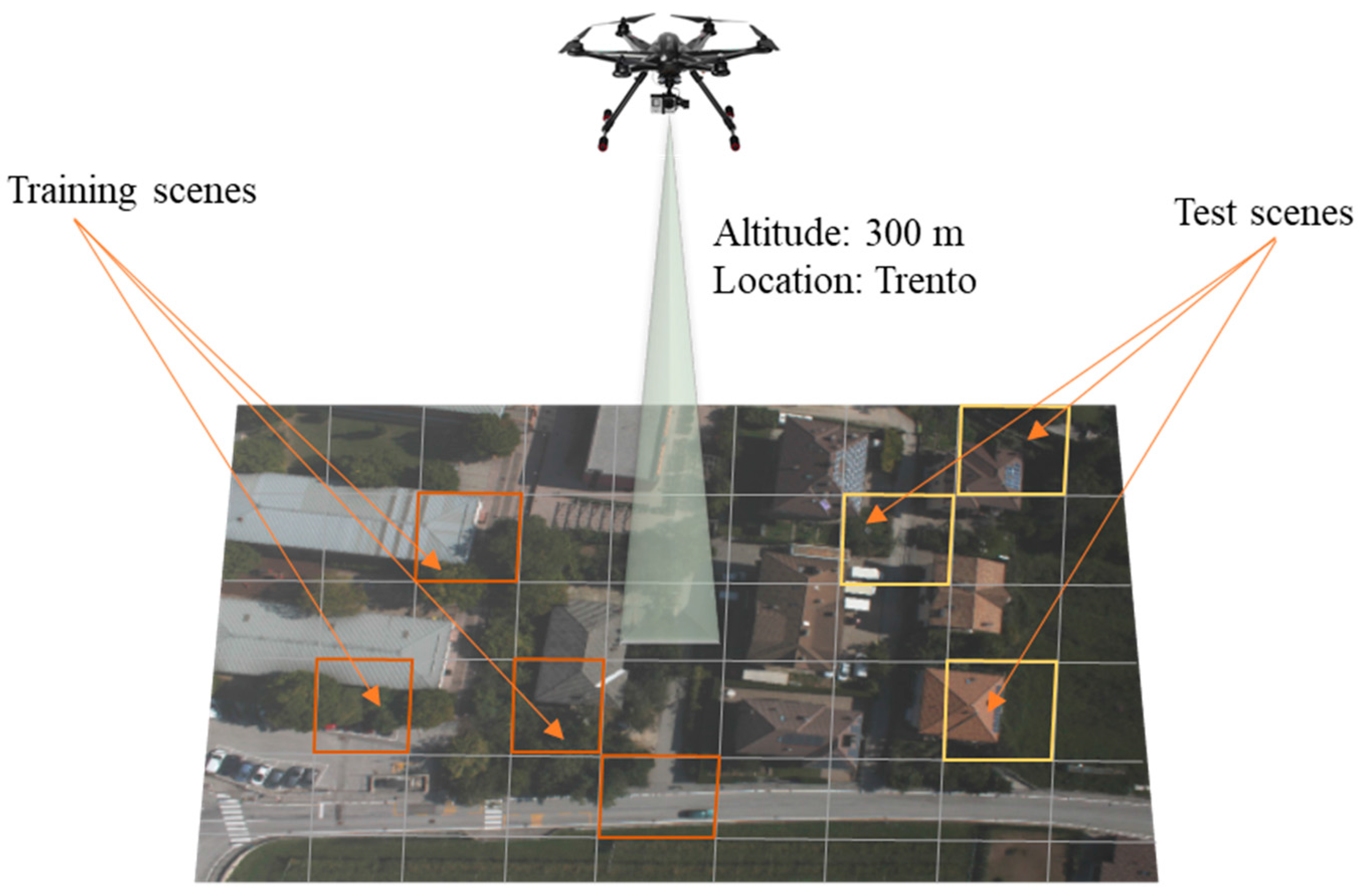
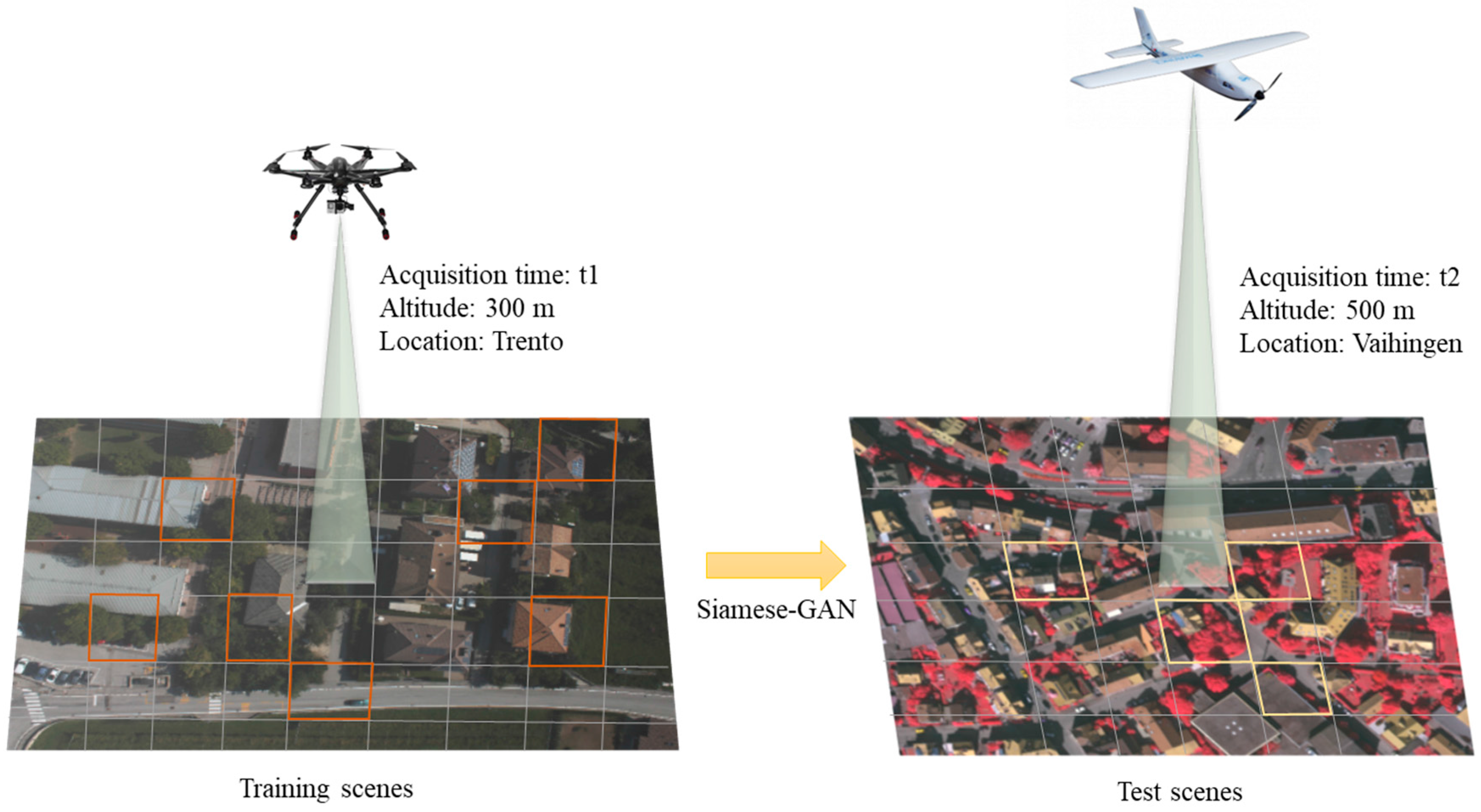
Figure 1 shows a typical situation in the case of UAV platform acquiring extremely high resolution images (EHR) over a specific area. However, in many real-world applications, the training images used to learn a model may have different distributions from the images used for testing. This problem arises when dealing with data acquired over different locations of the Earth’s surface and with different platforms, as shown in
Figure 2. We recall that this aspect is not obvious in the currently available scene datasets as the training and testing data are generated randomly during evaluation. To highlight this undesirable effect, the authors of [
37] have shown that the methods based on pre-trained CNNs may produce low accuracies when benchmarked with cross-domain datasets. As a remedial action, they have proposed compensating for the distribution mismatch by adding additional regularization terms to the objective function of the neural network besides the standard cross-entropy loss.
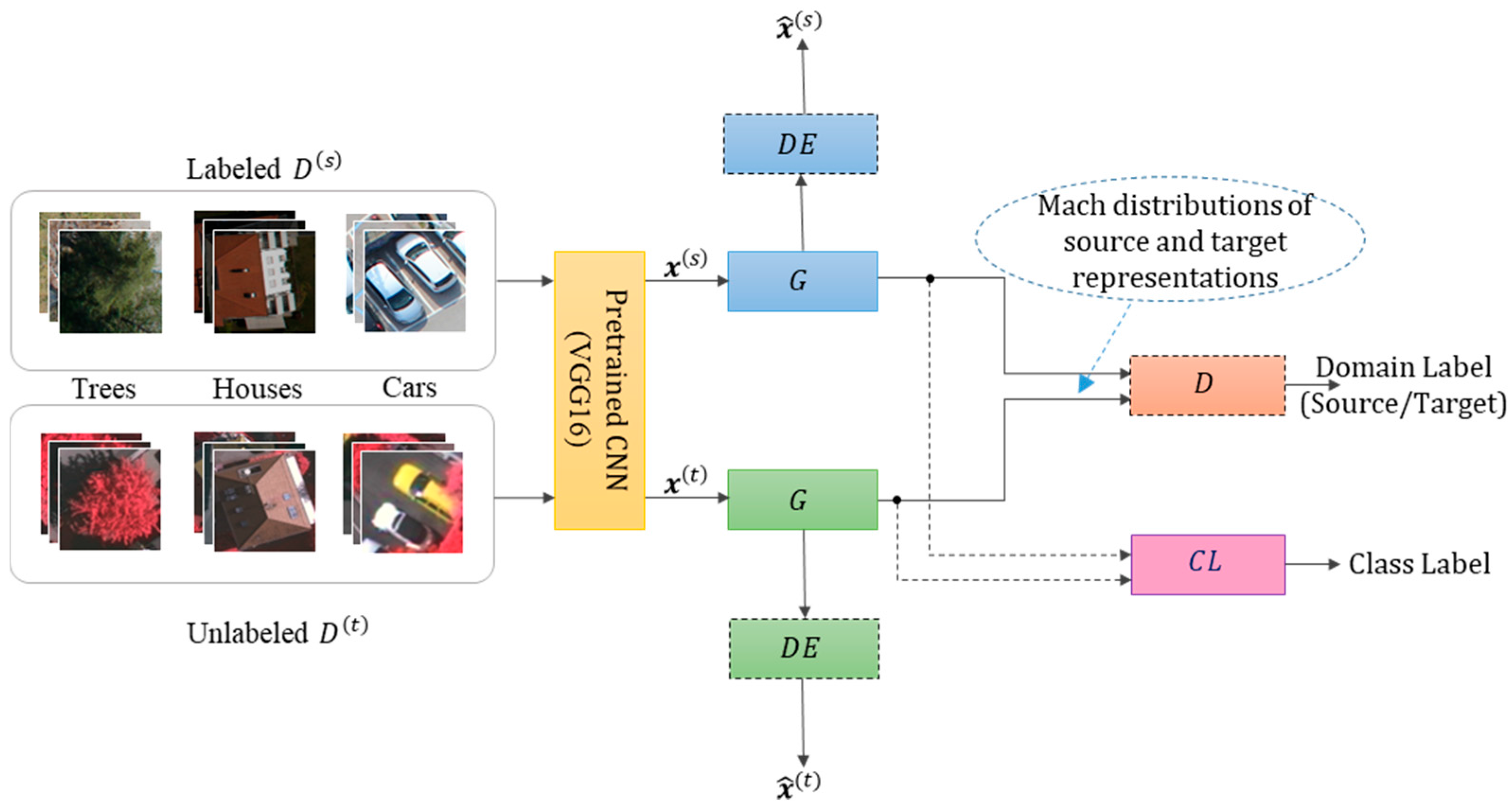
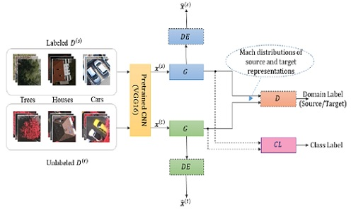
In this work, we propose a new domain adaptation approach to automatically handle such scenarios (
Figure 2). Our objective is to learn invariant high-level feature representations for both training and testing data coming from two different domains referred here for convenience as labeled source and unlabeled target data. The method, termed Siamese-GAN, trains jointly in an adversarial manner a Siamese encoder–decoder network coupled with another network acting as a discriminator. The encoder-decoder network has the task to match the distributions of both domains in a shared space regularized by the reconstruction ability, while the discriminator seeks to distinguish between them. At the end of the optimization process, we feed the resulting encoded labeled source and unlabeled target features into an additional network for training and classification, respectively.
The major contribution of this work can be summarized as follows: (1) Introduce GANs as promising solution for the analysis of remote sensing data. (2) Overcome the data-shift problem for cross-domain classification by proposing an efficient method named Siamese-GAN. (4) Validate the method on several cross-domain datasets acquired over different locations of the earth surface and with different MAV/UAV platforms. (4) Present a comparative study against some related methods proposed in the literature of remote sensing and computer vision.
The paper is organized as follows.
Section 2 reviews GANs.
Section 3 describes the proposed Siamese-GAN method.
Section 4 presents the results obtained for several benchmark cross-domain datasets.
Section 5 analyzes the sensitivity of the method and presents comparisons with state-of-the-art methods. Finally,
Section 6 concludes the paper.
2. Generative Adversarial Networks (GANs)
GANs have emerged as a novel approach for training deep generative models. The original GAN that was mainly proposed for image generation consists of two neural networks: the generator
and the discriminator
. The networks are trained in opposition to one another through a two-player minimax game. The generator network learns to create fake data that should come from the same distribution as the real data, while the discriminator network attempts to differentiate between the real and the fake data created by the generator. During each training cycle, the generator takes a random noise vector as an input and creates a synthetic image, the discriminator is presented with a real or generated image and tries to classify it as either “real” or “fake”. Ideally, the two networks compete during the training process until the Nash equilibrium is reached. The GANs’ objective function is given by:
where
represents the real image from the true data distribution
,
z represents the noise vector sampled from distribution
, and
represents the generated image. The generator
is learned by maximizing
, while
is trained by minimizing
.
Since the appearance of GANs in 2014, many extensions have been proposed to its architecture. For instance, Deep Convolutional GANs (DCGANs) [
38] were designed to allow the network to generate data with similar internal structure as training data, improving the quality of the generated images, and Conditional GANs [
39] add an additional conditioning variable to both the generator and the discriminator. Based on the previous architectures the concept of GANs has been adopted to solve many computer visions related tasks such as image generation [
40,
41], image super-resolution [
42], unsupervised learning [
43], semi-supervised learning [
44], and image painting and colorization [
45,
46].
In the context of domain adaptation, some works have recently been introduced to the literature of computer vision. For instance, Ganin et al. [
47] presented a domain-adversarial neural network method, which combines a deep feature extractor module with two classifiers for class-label and domain prediction, respectively. The network is trained by minimizing the label prediction loss for source data, and the domain classification loss for both source and target data via a gradient reversal layer. Liu and Tuzel [
48] introduced an architecture that couples two or more GANs, each corresponding to one image domain. The two generators share the weights of the first layers that decode high-level features to learn the joint distribution of the images in the two domains, while the discriminators share the weights of the last layers. The authors of [
49] proposed an architecture based on a CNN that is first trained with labeled source images. Then train in an adversarial manner a generator and a discriminator on source and target data. The domain adaptation is achieved by mapping the target data into the source domain using the trained generator. Then the mapped target data are classified using the CNN trained previously on the source data. In another work [
50], the authors proposed an adversarial training for unsupervised pixel-based domain adaptation to make synthetic images more realistic. The generator in this model uses the source images as input instead of the noise vector. The adaptation is achieved by transforming the source pixels directly to the target space, and the synthetic images help to maximize the accuracy of the classifier.
In the context of remote sensing, Lin et al. [
43] used GANs for unsupervised scene classification. The model consists of a generator that learns to produce additional training images similar to the real data, and a discriminator that works as a feature extractor, which learns better representations of the images using the data provided by the generator. In another work, He et al. [
44] proposed a semi-supervised method for the classification of hyperspectral images. Spectral–spatial features are extracted from the unlabeled images and are used to train a GAN model.
4. Experimental Results
4.1. Datasets Used for Creating the Cross-Domain Datasets
To evaluate the performance of the proposed method, we use four aerial datasets acquired with different sensors and altitudes and over diverse locations over the earth surface to build several benchmark cross-domain scenarios. Originally, these datasets were proposed for semantic segmentation and multilabel classification. Here, we tailor them to the context of cross-domain classification.
The first dataset was captured over Vaihingen city in Germany using Leica ALS50 system at an altitude of 500 m above ground level in July and August 2008. The resulting images are characterized by a spatial resolution of 9 cm. Each image is represented by three channels: near infrared (NIR), red (R), and green (G) channels. The dataset consists of three sub-regions: the inner city, the high riser and the residential area. The first area is situated in the center of the city, and is characterized by dense and complex historic buildings along with roads and trees. The second area consists of a few high-rise residential buildings surrounded by trees. The third area is a purely residential area with small detached houses and many surrounding trees.
The second dataset was taken over the central district of the city of Toronto in Canada by the Microsoft Vexcel’s UltraCam-D camera and the Optech’s airborne laser scanner (ALTM-ORION M) at an altitude of 650 m in February 2009. This dataset is located in a commercial zone that has representative scene characteristics of a modern mega city, containing buildings with a wide range of shape complexity in addition to trees and other urban objects. The resulting images have a ground resolution of 15 cm and RGB spectral channels.
The third dataset was acquired over the city of Potsdam using an airborne sensor. This dataset consists of RGB images with a ground resolution of 5 cm. Typically, this dataset contains several land cover classes such as buildings, vegetation, trees, cars, impervious surfaces, and other objects classified as background.
Finally, the Trento dataset consists of UAV images acquired over the city of Trento in Italy, on October 2011. These images were captured using a Canon EOS 550D camera with an 18 megapixels CMOS APS-C sensor. The dataset provides images with a ground resolution of approximately 2 cm and RGB spectral channels.
4.2. Cross-Domain Datasets Description
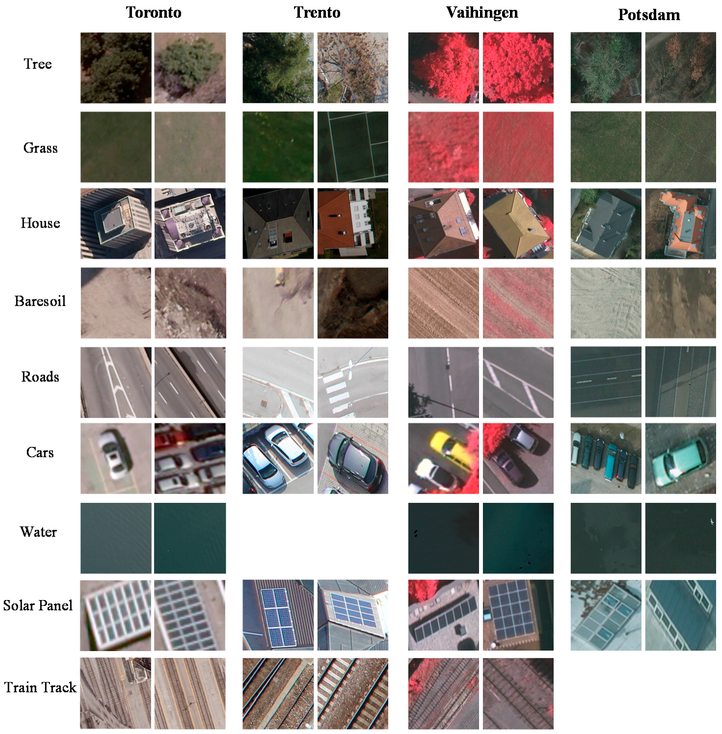
From the above four datasets, we build several cross-domain scenes by identifying the most common classes through visual inspection. For Toronto and Vaihingen, we identify nine common classes labeled as trees, grass, buildings, cars, roads, bare soil, water, solar panels, and train tracks. For the Trento and Potsdam datasets, we identified only eight classes, as the images for water and train track classes are unavailable for the first and second one, respectively.
Table 1 summarizes the number of images per class extracted for each dataset, while
Figure 6 shows some samples (cropped from the original images) normalized to the size 224 × 224 pixels. In the experiments, we refer to the resulting 12 transfer scenarios as source
target. For example, for the scenario Toronto
Vaihingen we have nine classes with 120 images per class. The total number of labeled source images and unlabeled target images used for learning is equal for both to 1080.
4.3. Experimental Setup
We implement the Siamese-GAN method in a Keras environment, which is a high-level neural network application programming interface written in Python. For training the related subnetworks, we fix the mini-batch size to 100 samples. Additionally, we set the learning rate of the Adam optimization method to . Regarding the exponential decay rates for the moment estimates and epsilon, we use the following default values 0.9 and 0.999 and respectively.
In the first set of experiments, we present the results by fixing the regularization parameter of the reconstruction loss to . Next, we provide a detailed sensitivity analysis of Siamese-GAN with respect to this parameter, besides other features related to the network architecture. Finally, we compare our results to several state-of-the-art methods. For performance evaluation, we present the results on the unlabeled target images using per-class accuracy through confusion matrices, the overall accuracy (OA), which is the ratio of the number of correctly classified samples to the total number of the tested samples, and the average accuracy (AA) for each method, which represents the sum of the OA obtained for all scenarios divided by 12 (i.e., AA = OA/12). The experiments are performed on a MacBook Pro laptop (processor Intel Core i7 with a speed of 2.9 GHz, and 8 GB of memory).
4.4. Results
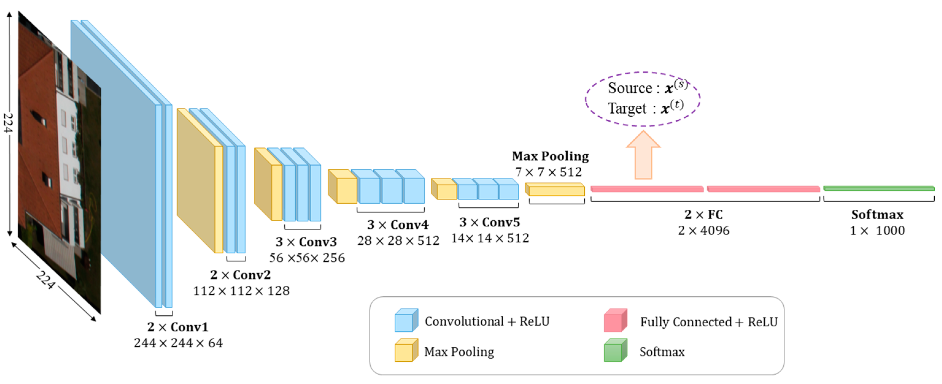
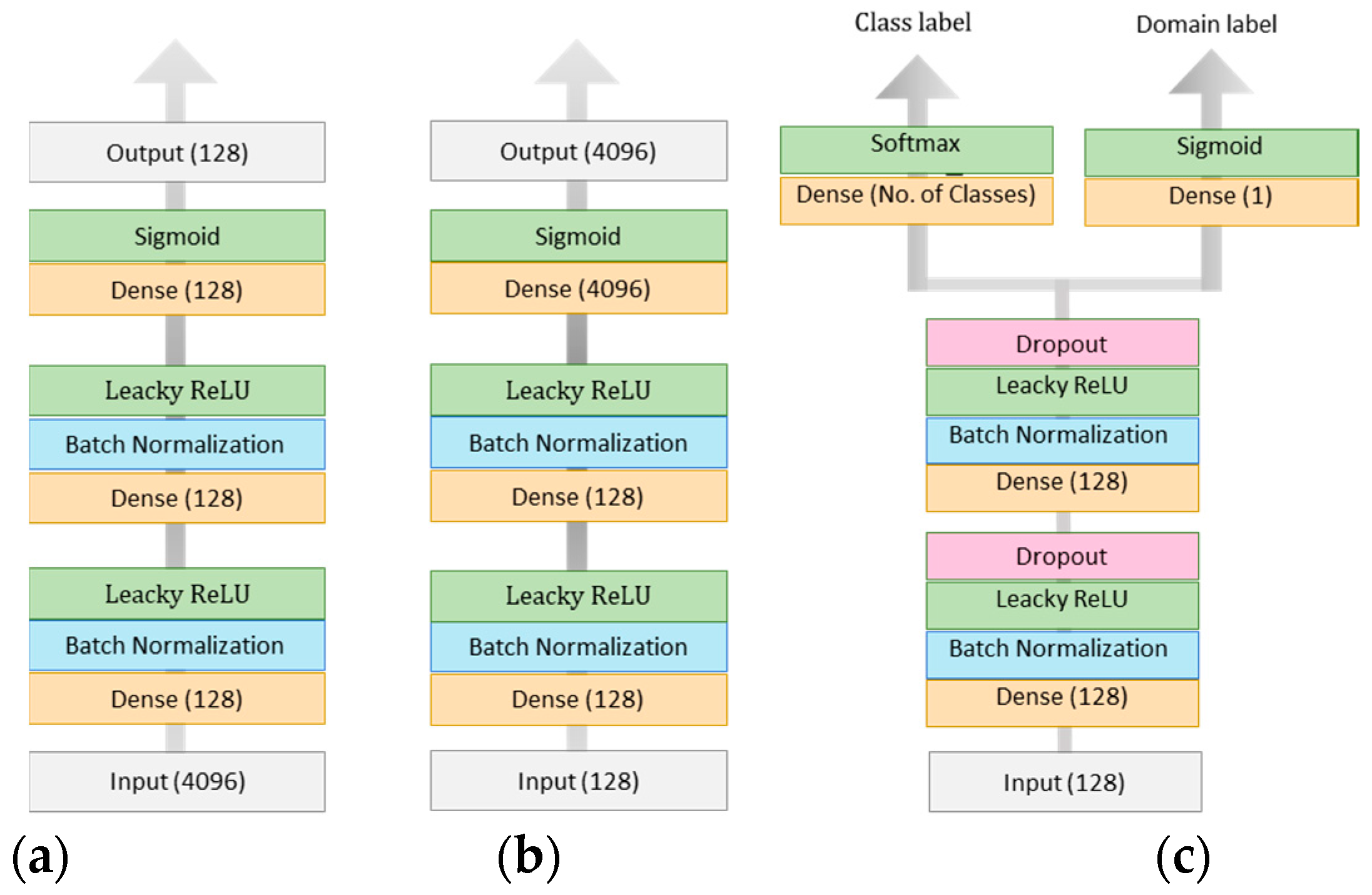
In this first set of experiments, we analyze the performance of our proposed method compared to the standard off-the-shelf classifiers solution. To this end, we first run the experiments by feeding the features extracted from VGG16 directly to an additional NN. This extra network has a similar architecture to the one shown in
Figure 5c.
Table 2 shows the classification accuracies for the 12 cross-domain scenarios. The lowest accuracy is obtained for Toronto
Vaihingen with an OA of 64.72%, while Potsdam
Trento shows the best result with an OA of 80.24%. Over the 12 scenarios, this solution yields an AA of 70.82%. We repeat these experiments using a linear multiclass SVM classifier with one-versus-one training strategy. We search for the best value of the regularization parameter according to a 3-fold cross-validation procedure in the range [10
−3 10
3]. In this case, the scenario Vaihingen
Potsdam shows relatively the lowest OA accuracy with 61.35%, while the best result is obtained for the scenario Potsdam
Trento with an OA of 86.55%. The average classification accuracy across the 12 scenarios is equal to 70.23%, which is very close to result obtained by the NN method.
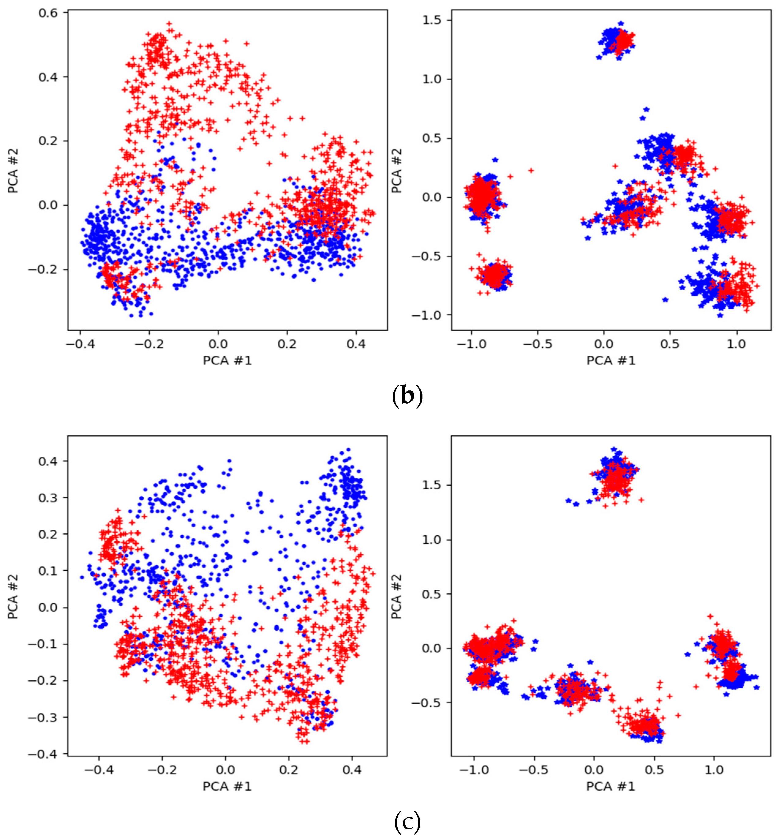
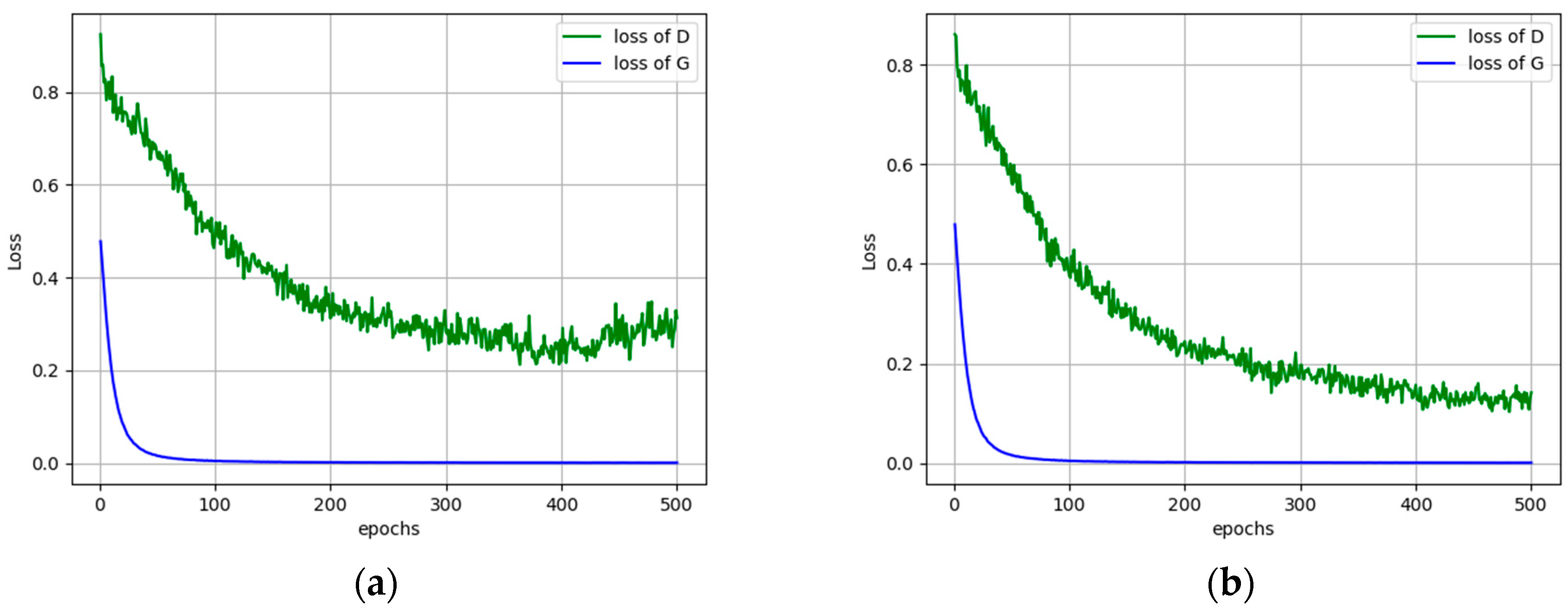
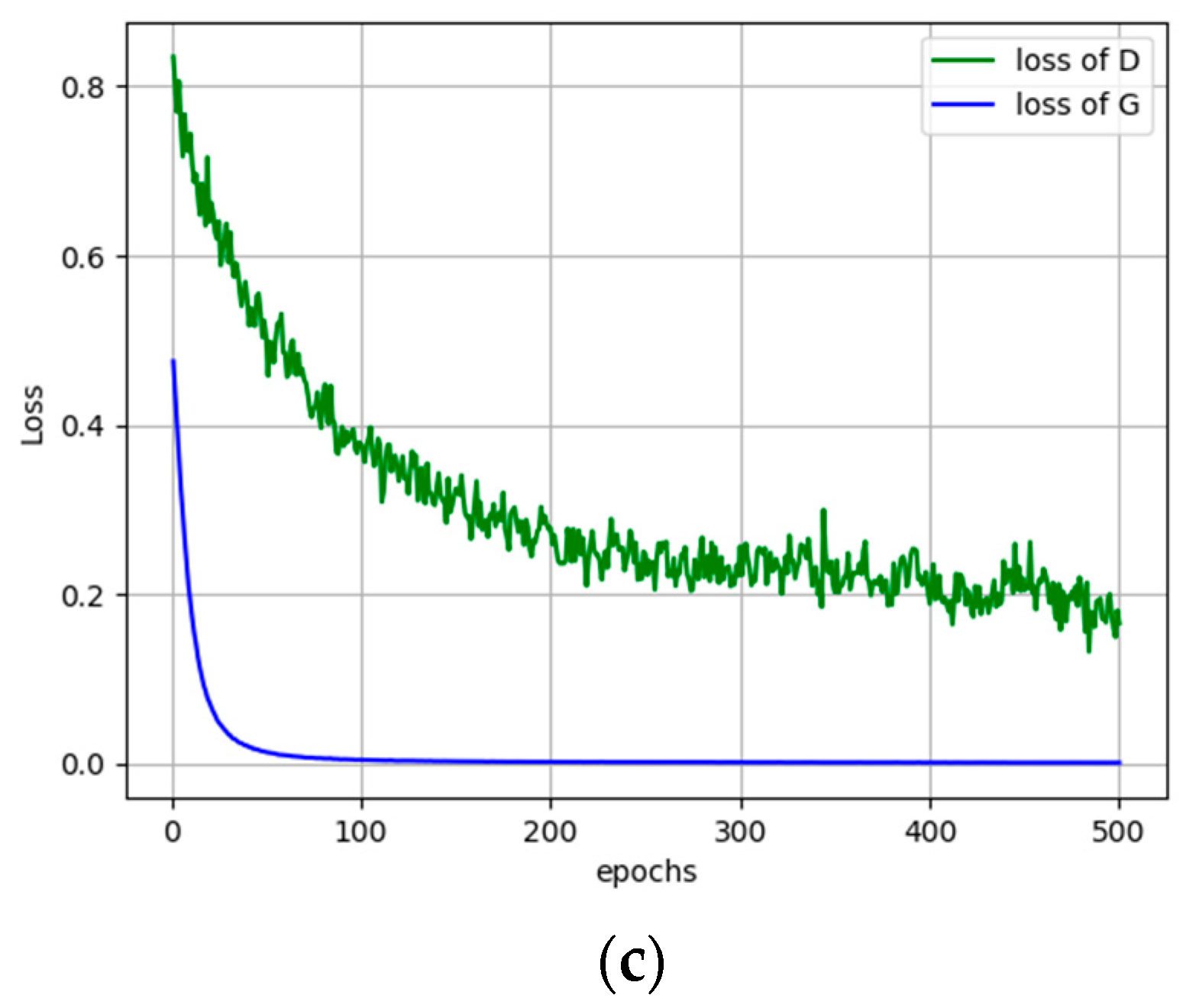
Next, we run the Siamese-GAN method as explained in
Section 3.3. In
Figure 7, we show the evolution of the Siamese encoder and discriminator losses. We recall that the Siamese encoder–decoder aims the match the distributions of both source and target while the discriminator seeks to discriminate them. The results reported in
Table 2 show clearly that it improves greatly the AA accuracy for all scenarios from 70.81% to 90.34%, which corresponds to an increase of around 19%. For certain scenario like Trento
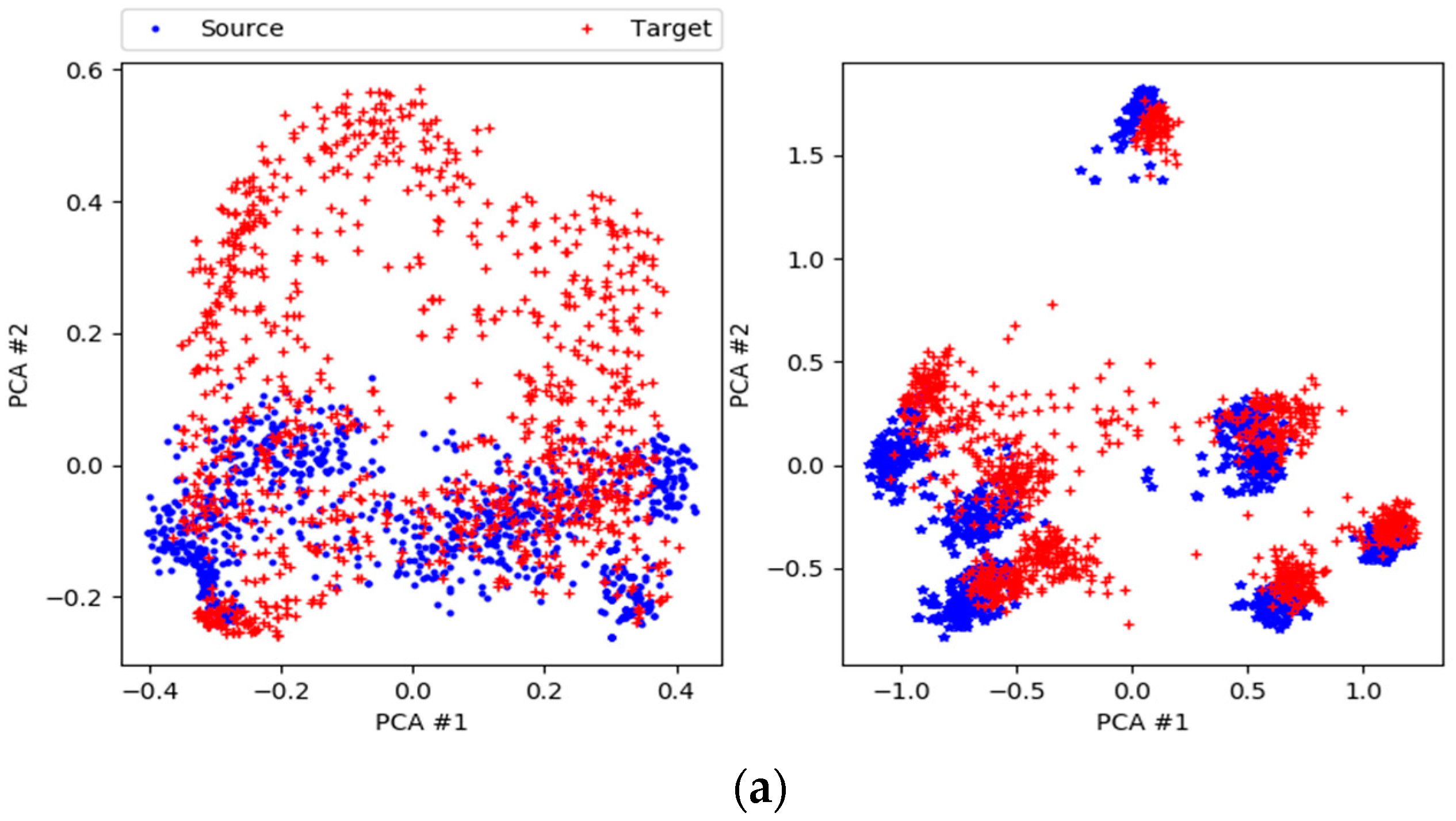
Vaihingen, it improves the OA by 28.85%. To understand better the behavior of the network, we show in
Figure 8 the data distributions before and after adaptation for three typical scenarios, which are Potsdam
Vaihingen, Toronto
Vaihingen, and Trento
Toronto, respectively. This figure shows that the shift between the source and target distributions is obvious before adaptation, which explains the low performance obtained by off-the-shelf classifier solution. However, this discrepancy is greatly reduced by Siamese-GAN, while keeping the discrimination ability between the different classes.
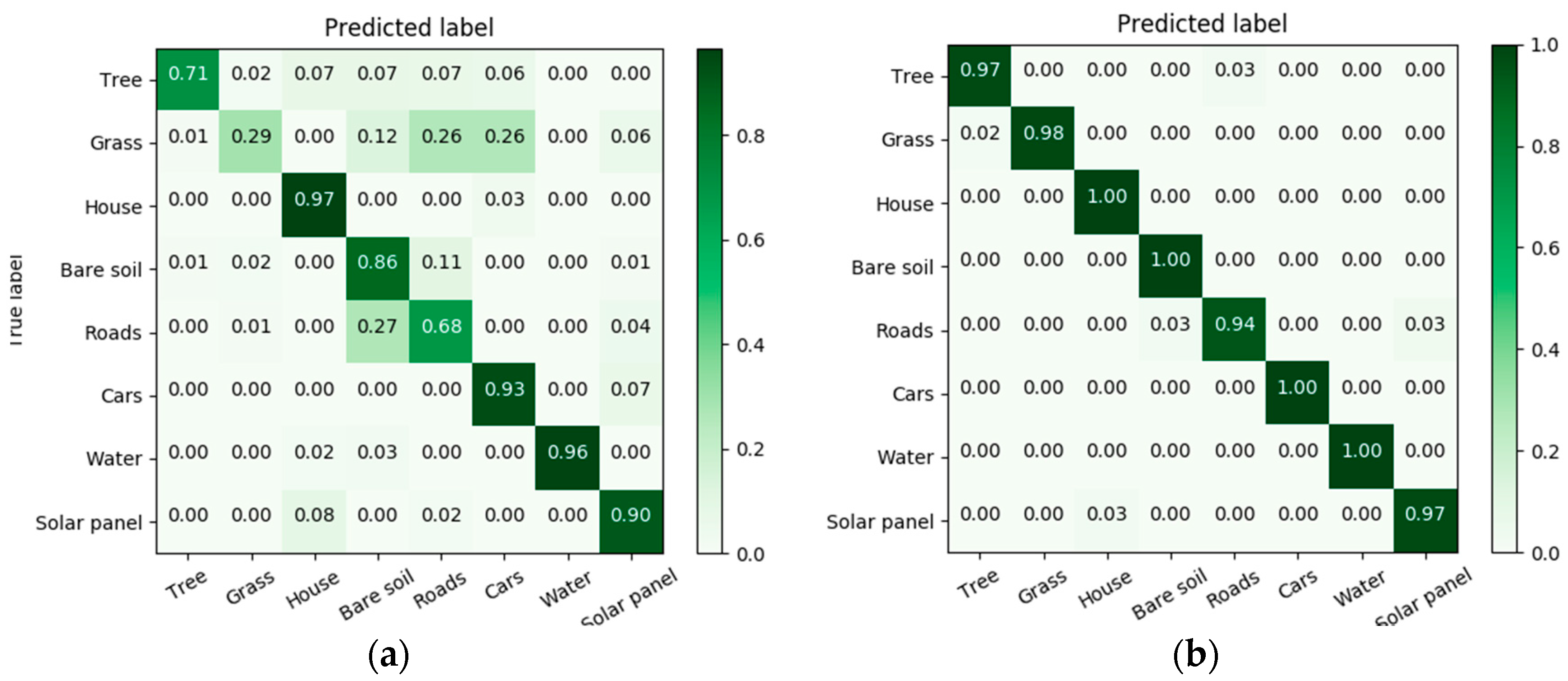
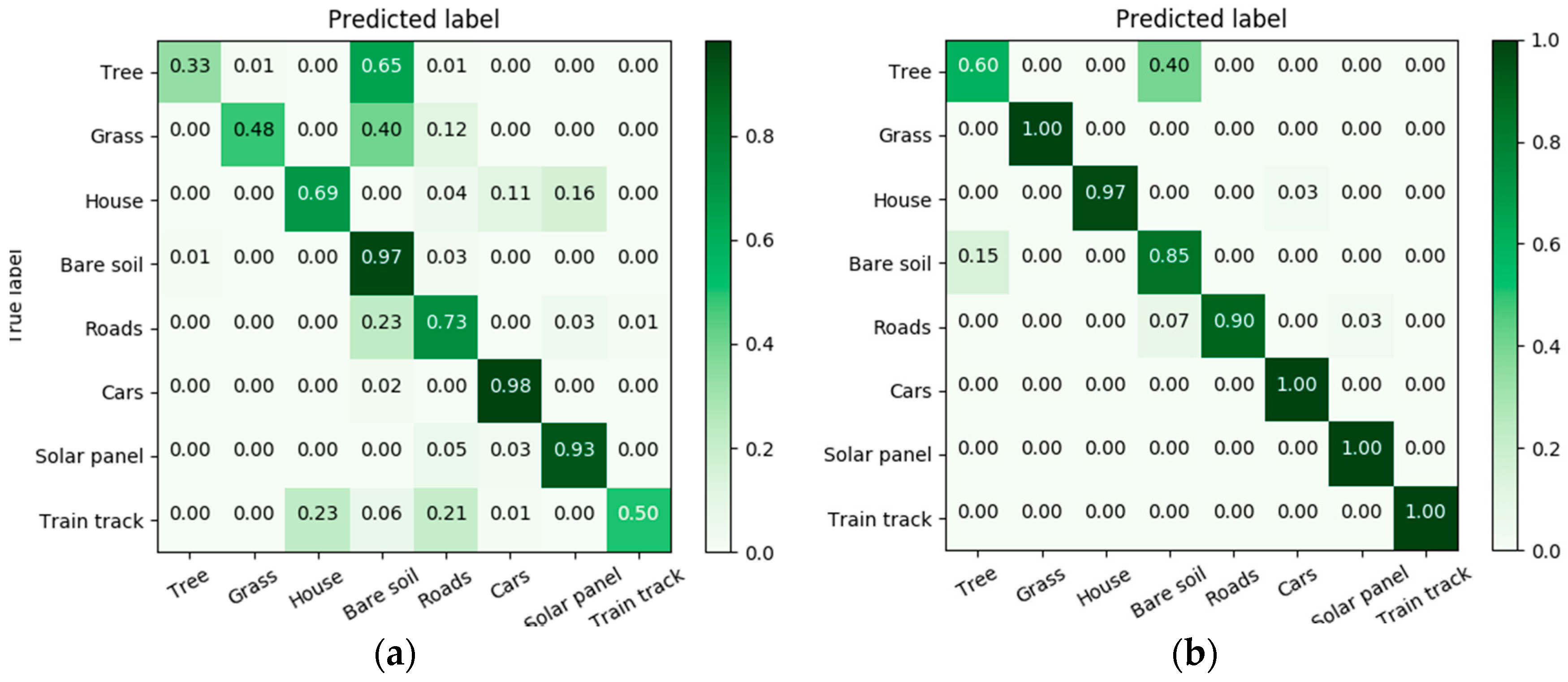
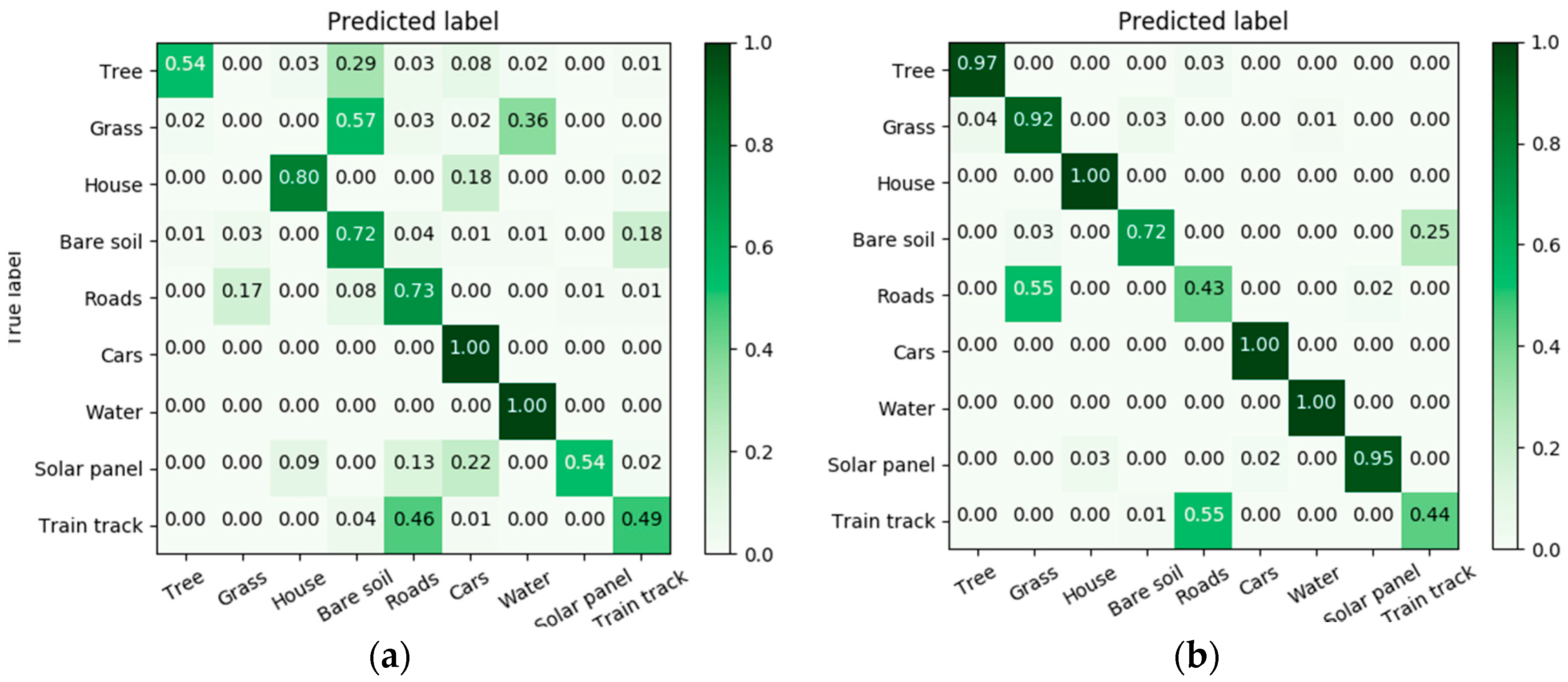
In
Figure 9,
Figure 10 and
Figure 11 we report the confusion matrices before and after adaptation. For example for Potsdam
Vaihingen, the accuracies of classifying some classes with (NN) such as Water and House were already high before adaptation (96% and 97%), and have been increased to 100% with adaptation. For classes with low accuracies such as Grass, more than 60% of the images were misclassified as either Roads, Cars or Bare soil. The result has been improved with adaptation from 29% to 98%, which is equal to 69% gain in accuracy. Additionally, the confusion between Roads and Bare soil has been reduced, resulting in an increase from 68% to 94%. For Trento
Toronto, before adaptation 65% of Trees samples were misclassified as Bare soil and the accuracy has increased after adaptation from 33% to 60%. On the other hand, the confusion between Grass and Bare soil classes has been resolved with adaptation, and the classification accuracy of the Grass class increases from 43% to 100%. For Toronto
Vaihingen, the accuracy of Grass samples has been greatly increased from 0% to 92% with adaptation. However, the Roads class accuracy dropped from 73% to 43%.


 ,
, 


