Spatiotemporal Analysis of Actual Evapotranspiration and Its Causes in the Hai Basin


1
Key Laboratory of Digital Earth Science, Institute of Remote Sensing and Digital Earth, Chinese Academy of Sciences, Olympic Village Science Park, W. Beichen Road, Beijing 100101, China
2
College of Resources and Environment, University of Chinese Academy of Sciences, Beijing 100049, China
*
Author to whom correspondence should be addressed.
Remote Sens. 2018, 10(2), 332; https://doi.org/10.3390/rs10020332
Submission received: 2 December 2017
/
Revised: 22 January 2018
/
Accepted: 12 February 2018
/
Published: 23 February 2018
(This article belongs to the Section Remote Sensing in Geology, Geomorphology and Hydrology)
Abstract
:Evapotranspiration (ET) is an important component of the eco-hydrological process. Comprehensive analyses of ET change at different spatial and temporal scales can enhance the understanding of hydrological processes and improve water resource management. In this study, monthly ET data and meteorological data from 57 meteorological stations between 2000 and 2014 were used to study the spatiotemporal changes in actual ET and the associated causes in the Hai Basin. A spatial analysis was performed in GIS to explore the spatial pattern of ET in the basin, while parametric t-test and nonparametric Mann-Kendall test methods were used to analyze the temporal characteristics of interannual and annual ET. The primary causes of the spatiotemporal variations were partly explained by detrended fluctuation analysis. The results were as follows: (i) generally, ET increased from northwest to southeast across the basin, with significant differences in ET due to the heterogeneous landscape. Notably, the ET of water bodies was highest, followed by those of paddy fields, forests, cropland, brush, grassland and settlement; (ii) from 2000 to 2014, annual ET exhibited an increasing trend of 3.7 mm per year across the basin, implying that the excessive utilization of water resources had not been alleviated and the water resource crisis worsened; (iii) changes in vegetation coverage, wind speed and air pressure were the major factors that influenced interannual ET trends. Temperature and NDVI largely explained the increases in ET in 2014 and can be used as indicators to evaluate annual ET and provide early warning for associated issues.

1. Introduction
Evapotranspiration (ET), which involves the evaporation of water from water bodies and land surfaces and transpiration through plants, is a very important component of the hydrological cycle [1,2,3]. Approximately 60 to 65% of precipitation returns to the atmosphere and hydrological cycle through ET [4,5,6], particularly in arid and semi-arid areas, where 90% of precipitation is involved in ET processes [7]. A comprehensive understanding of the spatiotemporal pattern of ET can provide effective information for irrigation scheduling, hydrological model applications, and assessments of the sustainable utilization of water resources [8,9,10,11,12].
Accurate ET data are fundamental and crucial in spatiotemporal characteristic analysis. At the field scale, measures such as the eddy covariance (EC) and Bowen ratio are employed, and micrometeorological models are used to estimate actual ET [13,14,15,16,17]. However, these methods only provide estimates of ET over small areas rather than the watershed scale [18]. Remote sensing (RS) provides temporally continuous and large-scale information over the land surface. Land surface biophysical properties can be derived from this information using normalized difference vegetation index (NDVI), albedo, land surface temperature and roughness information. In recent years, traditional ET models and RS parameters have been combined and widely used in different regions [19,20,21,22,23]. Bastiaanssen [19,23] and Su [21] developed the SEBAL and SEBS models, respectively, for estimating actual ET (heavily relying on RS data). However, cloud cover and data quality problems in optical RS data result in data gaps and inaccurate ET estimates on unclear days [18]. Therefore, to overcome these challenges, models such as ETWatch [18] and MOD16 [24] have been proposed to estimate daily ET through the combination of RS information and the Penman-Monteith equation. The MOD16 algorithm is based on the Penman-Monteith equation [25] and retrieves canopy resistance from stomatal conductance, the leaf area index (LAI) and the vapor pressure deficit (VPD) [20]. Mu evaluated the MOD16 data set using data from 46 EC stations in America and concluded that the mean bias of daily ET was 0.31 mm/day, or 24% of the ET measured in situ [24]. ETWatch model combines the surface energy balance and Penman-Monteith equation, and the daily surface resistance estimation was a key step to estimate daily ET (details of the temporal scaling of surface resistance will be discussed in Section 3.1). ETWatch was validated in the Hai Basin using soil moisture depletion, EC and lysimeter data. Notably, the seasonal bias was 12% and decreased to 6% over an annual cycle at individual field sites, and the deviation was 3% for an annual cycle in the Hai Basin [18].
Li et al. analyzed the spatiotemporal variation of ET using the complementary relationship method and data from 31 meteorological stations in the Hai Basin from 1961 to 2010. They found that ET exhibited a significant negative trend at a rate of 12.5 mm/10 years [26]. To quantitatively evaluate the impact of climate change on ET, Liu et al. assessed the ET trend from 1961 to 2006 using the SPS model and observed that climate change contributed to a change of −16.62 × 10⁹ m3, and ET was affected by precipitation rather than potential evapotranspiration (ET) in the Yellow River Basin [11]. To quantify the effects of climate variability and human activities on the hydrological system of the Hai Basin, Lu et al. explored the trends of hydrological elements, such as precipitation and evapotranspiration, and found that climatic variability dominated the changes in the hydrological system from 1989 to 2008 [27]. Liu et al. used an Integrated Dynamic Land Ecosystem Model (MLEM) in conjunction with landcover change and concluded that cropland-related land transformation was the dominant anthropogenic force affecting water resource during 20th Century [28]. In North China Plain, Hu et al. employed soil water balance model to access the changes of ground water and draw a conclusion that 29.2% or 135.7 mm reduction in irrigation could stop groundwater drawdown in the plain [29].
Analyses are required to understand the causes of spatiotemporal variations. Classical correlation and detrended fluctuation analyses are two effective methods of analyzing such variations. Detrended analysis can quantify the contributions of variables with significant trends. By removing significant increases or decreases and recalculating the reference ET with the detrended data set, several papers have analyzed the contributions of climatic variables to reference ET or actual ET [11,30,31,32,33]. For example, Xu found that a decrease in net total radiation was the main cause of the decrease in reference ET in the Yangtze catchment from 1960 to 2000 [30].
Previous research on spatiotemporal variations has been largely based on meteorological station data [11,26,30,32,34], which may result in misleading spatiotemporal characteristics at the regional scale; however, RS data can be used to explain these variations. Recently, with urbanization [35,36] and landscape changes [37] in China, the water resource crisis has become increasingly severe [38]. The Hai Basin is one of the regions facing serious water resource problems and groundwater exploitation issues, which have led to the decline of the ground table below the alluvial plain [39]. The objectives of this study are to investigate the effects of landscape change on the spatiotemporal pattern of ET in the Hai Basin and to analyze the current water resource crisis to improve water resource management and decision making. This research will provide a blueprint for RS analyses of ET that can be applied for water resource monitoring in other basins or regions.
2. Data and Study Area
2.1. The Hai Basin
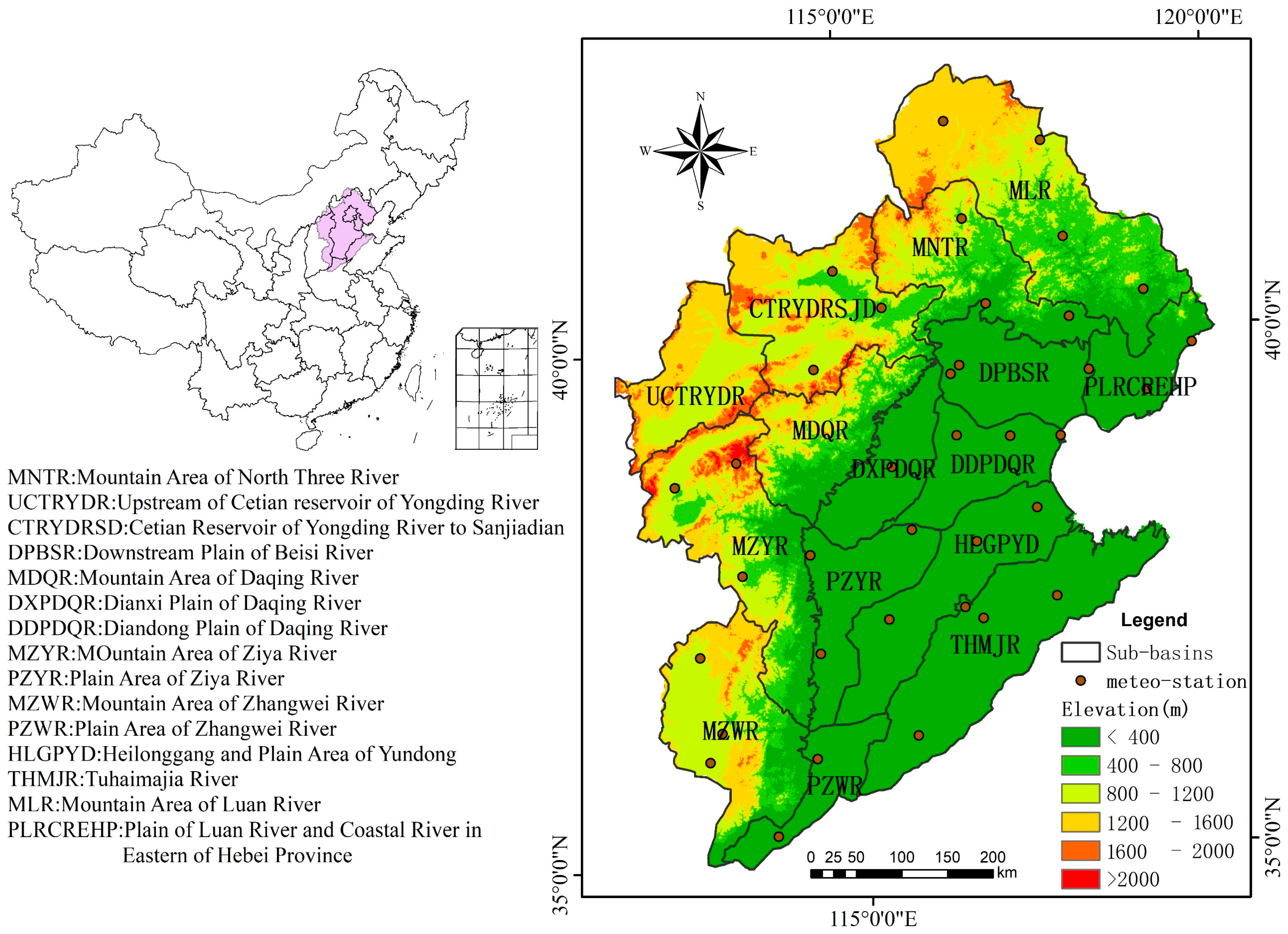
The Hai Basin is adjacent to the Bohai Sea and stretches from 35° to 43°N and 112° to 120°E (Figure 1). Originating on the Mongolian Plateau, the Loess Plateau, Mount Taihang and Mount Yan, the Hai River flows through the North China Plain and finally empties into the Bohai Sea. The Hai Basin encompasses the Luan, Haihe and Tuhaimajia River plains and covers an area of approximately 318,000 km2, or 3.3% of China’s territory [26].
The average elevation of the Hai Basin is 584 m (Figure 1), and the areas covered by plains, hills and mountains are 200,000 km2, 83,000 km2 and 34,000 km2, respectively. The Hai Basin is located in a temperate semi-humid, semi-continental monsoon climate zone. The regional climate is hot and wet in summer and dry and cold in winter. This region receives the lowest rainfall of the eastern coastal areas of China. Specifically, the average annual rainfall in the Hai Basin is merely 557 mm year−1 [10].
This basin contains 15 subbasins (Figure 1), and most are located in the southeastern Hai Basin, including PLRCREHP, DPBSR, DXPDQR, DDPDQR, PZYR, HLGPYD, THMTR and PZWR. These subbasins are characterized by cropland and settlement. The western Hai Basin, including MLR, MNTR, CTRYDRSD, UCTRYDR, MDQR, MZYR and MZWR, is characterized by forest, brush, and grassland landscapes, with few cropland and settlement.
2.2. Data
The MOD021KM and MOD03 data sets were obtained from the NASA Goddard Space Flight Center (GSFC) and Atmosphere Archive and Distribution System (LADDS) [40]. MOD021KM is Level 1B Calibrated Radiances dataset, which contains calibrated and geolocated at-aperture radiances for 36 discrete bands located in the 0.4 µm to 14.4 µm region of the electromagentic spectrum [41]. MOD03 contains the geolocation dataset, which are calculated for each 1 km MODIS Instantaneous Field of Views (IFOV) for all orbits daily. MOD03 include geodetic latitude, longitude, solar zenith and azimuth angles, satellite zenith and azimuth angles, which are used to estimate net solar radiation [12]. More detail information about MODIS can be found in https://ladsweb.modaps.eosdis.nasa.gov/. Absolutely cloud-free Aqua MODIS images from 2000 to 2014 were used for ET calculation. The 6S model was used to calibrate for atmospheric effects using the lookup table method based on the aerosol optical thickness [42]. A practical split-window approach was employed to retrieve the land surface temperature (LST) [43,44].
Diurnal meteorological data from 57 meteorological stations (Figure 1) were obtained from the Meteorological Center of the National Meteorological Bureau. These data included sunshine hours, air temperature, air pressure, air humidity, and wind speed, which were interpolated to daily maps at a 1-km resolution using the inverse distance squared method with DEM data [45].
3. Methods
3.1. ETWatch
ETWatch is an ET monitoring system based on the surface energy balance and Penman-Monteith equation. The energy balance model is used to estimate surface fluxes on sunny days, and the Penman-Monteith approach is employed to calculate daily ET based on meteorological data and surface resistance determined from the results of an energy balance model on non-cloudy days. A detailed description of ETWatch and its accuracy were published by Wu et al. [18]. The working procedure of ETWatch is illustrated in Figure 2.
The surface energy balance equation [19], also called the “Residue Approach”, can be simplified as follows:
where Rn is the net radiation flux absorbed at the land surface, G0 is the soil heat flux conducted downward, H is the sensible heat flux warming the air and is the latent heat flux associated with evapotranspiration (all these fluxes are in W m−2).
The Penman-Monteith equation described by Monteith [25] can be expressed as follows:
where λE (W m−2) is the latent heat flux, λ is the latent heat of evaporation, is the slope of the curve relating the saturated water vapor pressure and temperature, Rn is the net radiation flux, G0 is the soil heat flux, ρ (kg m−3) is the air density, Cp (J kg−1 K−1) is the specific heat of air, [48] is vapor pressure deficit (VPD), γ (Pa K−1) is the psychrometric constant, ra is aerodynamic resistance, and rs is surface resistance.
The aerodynamic roughness length (Z0m) is an important parameter for determining ra. Most ET models are based on a smooth surface and do not consider the influence of vegetation height on roughness or use empirical coefficients dependent on land use. However, their accuracy of such methods is poor in hilly areas. The calculation of Z0m in ETWatch considers the vegetation cover and hypsography.
In ETWatch, the daily surface resistance (rs,daily) is extended from rs on neighboring cloud free days and is given as follows:
where is the daily bulk stomatal resistance of a well-illuminated leaf, is a daily data set of LAI, is the daily soil moisture, is on clear days, is LAI on clear days based on satellite data, is soil moisture retrived from AMSRE data on clear days, m(Tmin) is the minimum air temperature, and m(VPD) is the vapor pressure deficit.
3.2. Temporal Trend Analysis
To evaluate the temporal trends of ET data series and factors such as NDVI, albedo, sunshine hours (Sunt), average air temperature (Tavg), air pressure, wind velocity (Winv), and relative humidity (Humd), a parametric t-test [49] and nonparametric Mann-Kendall test were performed.
The t-test was introduced in 1908 by William Sealy Gosset and has been widely used in tests of the null hypothesis [50]. The simple linear least squares regression equation is given as follows:
where and are least squares intercept and slope, respectively; is the time (day or year); and is the estimated outcome, which is the predicted ET in this study. The sum of squares of residuals (SSR) is as follows:
where is the estimated outcome and is the tested time series, which is the actual ET from 2000 to 2014 in this study. Then, T is given by the following expression:
where T is the hypothesis test statistic (and follows a T distribution), n is the number of X, and is the average of X. is often taken to be 0, in which case the null hypothesis is that x and y are independent. The null hypothesis is rejected at a significance level of α if , where , n = 15, and T = 2.16.
The Mann-Kendall (M-K) method, which was developed by Mann and refined by Kendall [51,52], has been widely used to evaluate hydrological and climatological trends [48,53,54,55]. In this study, the M-K method is used to assess the temporal trend of ET and detect abrupt changes in ET at the annual scale.
3.3. Detrended Analysis
- (1)
- The significant linear trends in meteorological and RS parameters were removed. Specifically, the linear trend was calculated using least squares regression:where is a time series over and are coefficients in the least squares regression, is the prediction result and is the detrended stationary time series.
- (2)
- ET was derived from ETWatch using one detrended parameter and original data for other parameters.
- (3)
- The ET recalculated using detrended parameters was compared with the original ET, and the difference was considered the contribution of the parameter.
4. Results
4.1. The Spatial Distributions of ET and Land Cover
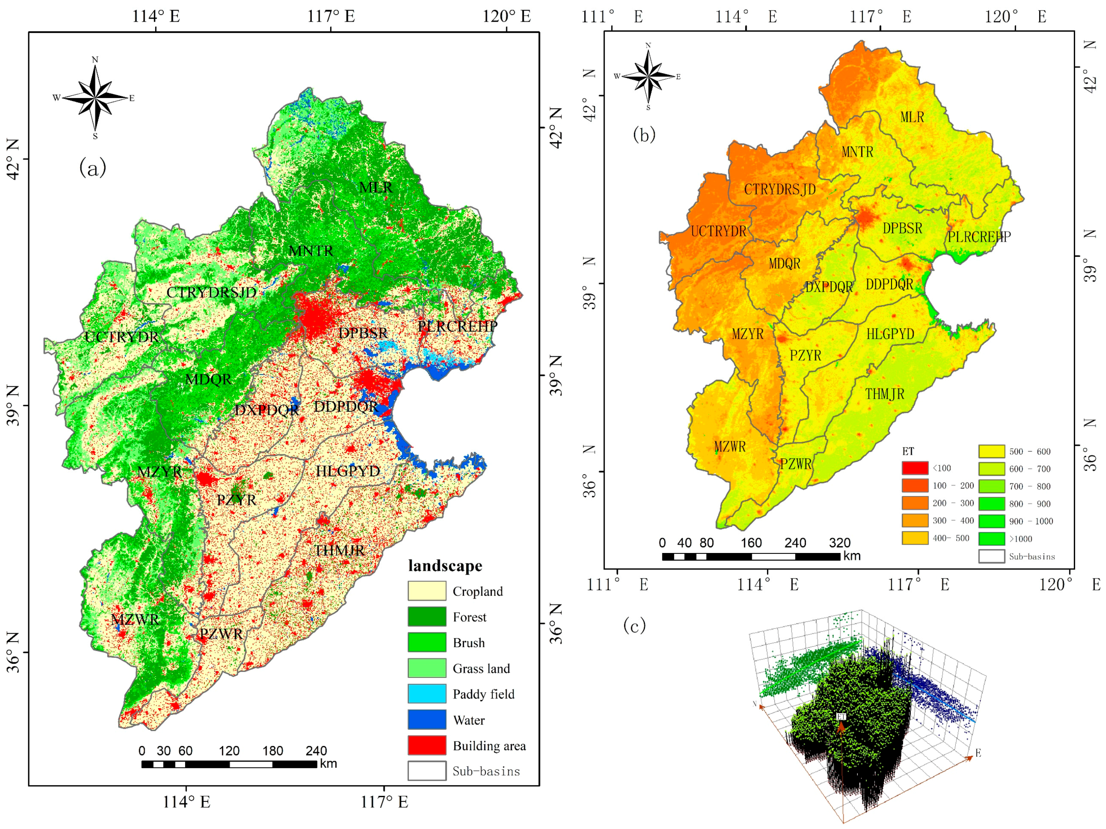
The spatial distribution map of ET in the Hai Basin (see Figure 3b) shows that the highest values are in areas close to Bohai Bay, while the lowest are in settlement. Generally, ET was lower in the western mountain areas and higher in the eastern plains. Here, the ET raster data were smoothed using a low-pass 3-by-3 filter, and ET was extracted at points using a 10-km interval. Then, the distribution trend was analyzed using the ArcGIS Geo-statistical analysis tool (Figure 3c), and the results show a clear increasing trend from northwest to southeast.
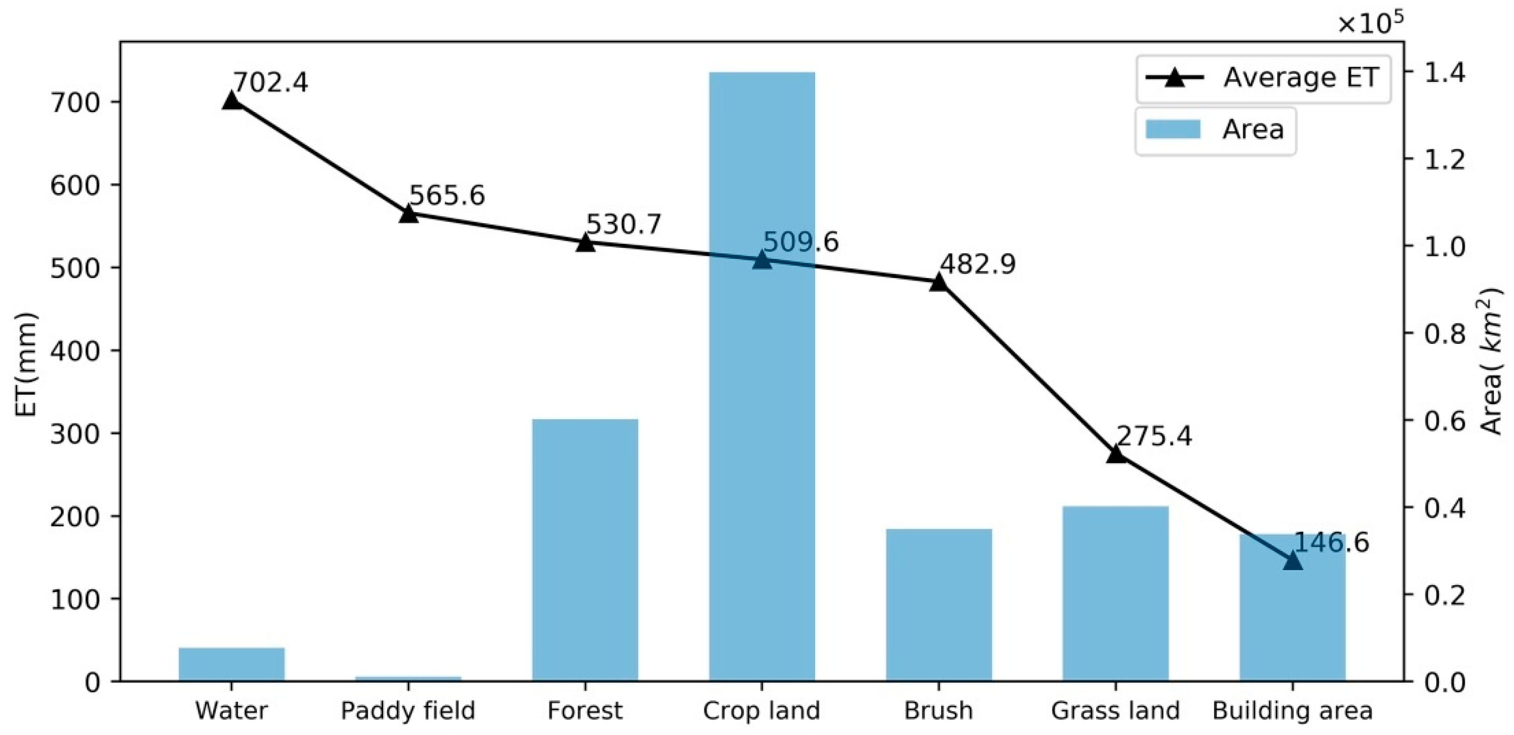
ET varies based on the landscapes, and the average ETs of different land covers are illustrated in Figure 3b. The ET of water is highest, followed by those of paddy fields, forests, cropland, brush, and grassland, and settlement have the lowest ET. The main land cover types are grassland in the Inner Mongolia dam area, deciduous forest in mountain areas and cropland on the alluvial plains of the Hai River (Figure 3a). The proportion of agricultural land is closely related to the population [56]. Notably, 150 million people live in this region and account for close to 10% of the total population of China. Expansive cropland is needed to sustain this population, and the area of cropland is approximately 140,000 km2, followed by the areas of forest, grassland, brush, and settlement (Figure 4). Considering these areas and the ET per unit area, cropland loses the most water via ET at approximately 50.1%, followed by forests at approximately 22.4%, brush at 11.9%, grassland at 7.8% and other land cover types at 7.8%.
Evapotranspiration from cropland and forest areas accounted for approximately 72.5% of ET in the Hai Basin. The average ET in cropland areas was 509.6 mm, with the highest value in PZYR, followed by those in THMJ, HLGPYD, PZWR, DXPDQR, DPBSR, PLRCREHP and DDPDQR. This difference may result from the variable climate conditions and crop types. For example, the ET of winter wheat rotated with corn is larger than that of a single cropping system, such as cotton or corn. The average ET in forest areas was 530.7 mm, with the highest value in MNTR, followed by those in MLR, CTRYDRSJD, MZWR, MZYR, MDQR, and UCTRYDR. ET in forest areas may vary based on the climate conditions and tree species; for example, the ET in broad-leaved forest areas is larger than that in coniferous forest areas.
4.2. The Temporal Change in ET
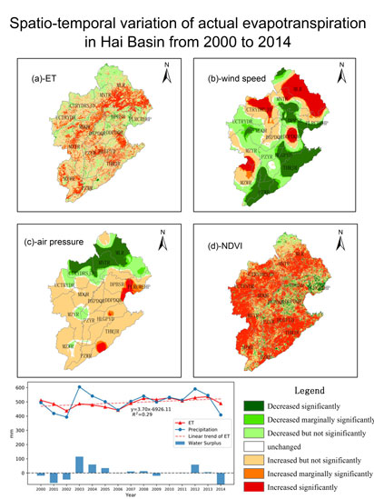
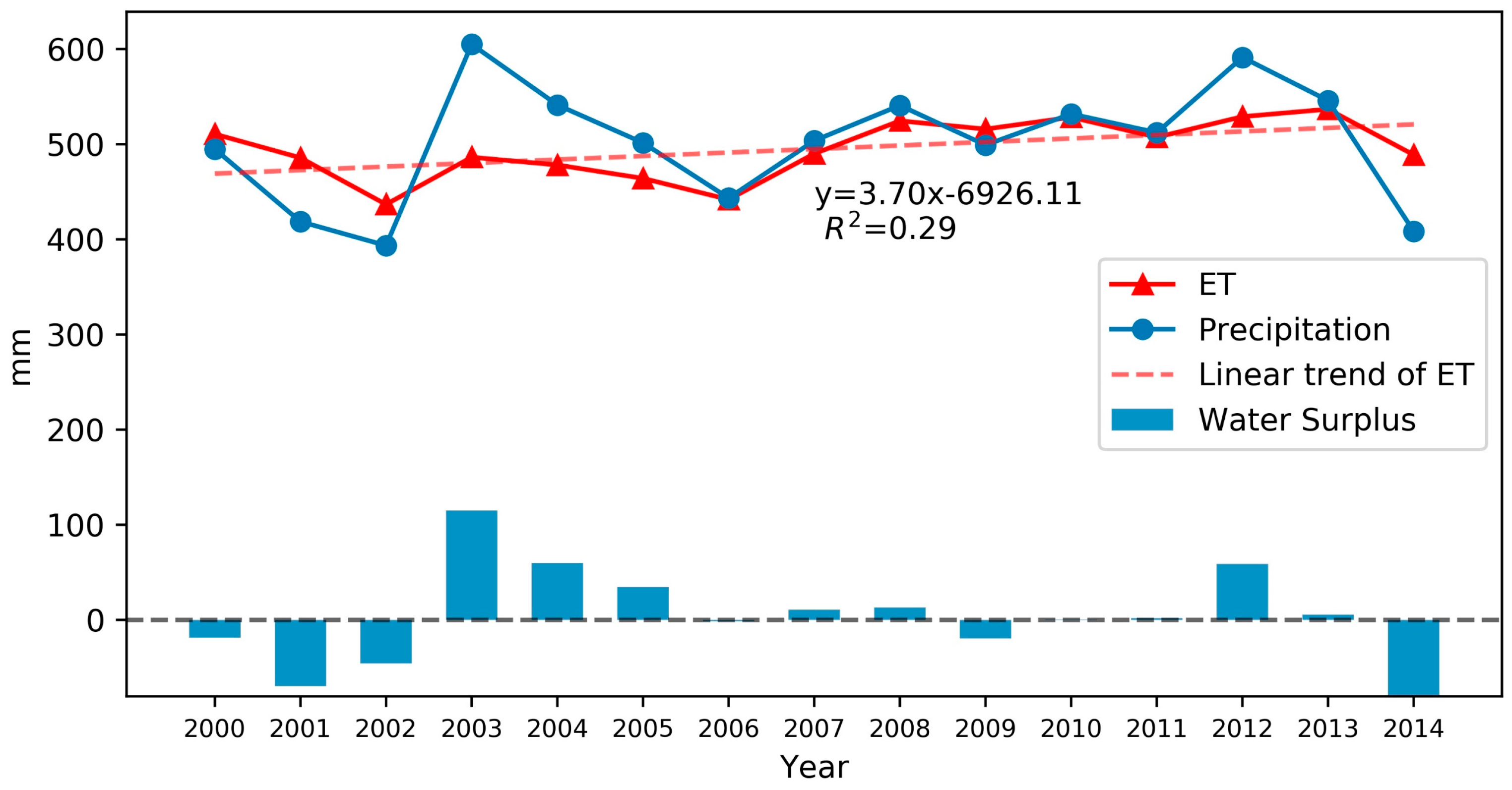
Figure 5 illustrates the trends of ET, water surplus (the difference between precipitation and ET) and precipitation from 2000 to 2014. To assess the temporal trends at the interannual scale, both a nonparametric M-K test and a parametric t-test were performed (Table 1). In the M-K test and t-test, the statistic variable Z of ET was 2.18, and T was 2.28 in the t-test. Additionally, ET was significant () and increased with a slope of 3.70 from 2000 to 2014. Fei et al. concluded that the Hai Basin would experience an increase in evaporation and a warmer climate in the future [57]. Precipitation increased, but not significantly (T = 0.79, Z = 0.99), and exhibited a smaller slope (3.00 mm per year) than ET in this period. The water surplus remained stable or minimally decreased (−0.65 mm per year) at a low confidence level (T = −0.21, Z = 0). In this period, the NDVI increased significantly at a rate of 0.002 per year in the Hai Basin. This finding was consistent with those of previous studies and may result from increased precipitation and ecological restoration projects [37,58,59,60]. Other meteorological factors changed but not significantly. Therefore, the increase in ET could have resulted from the increase in the NDVI from 2000 to 2014 in the entire basin.
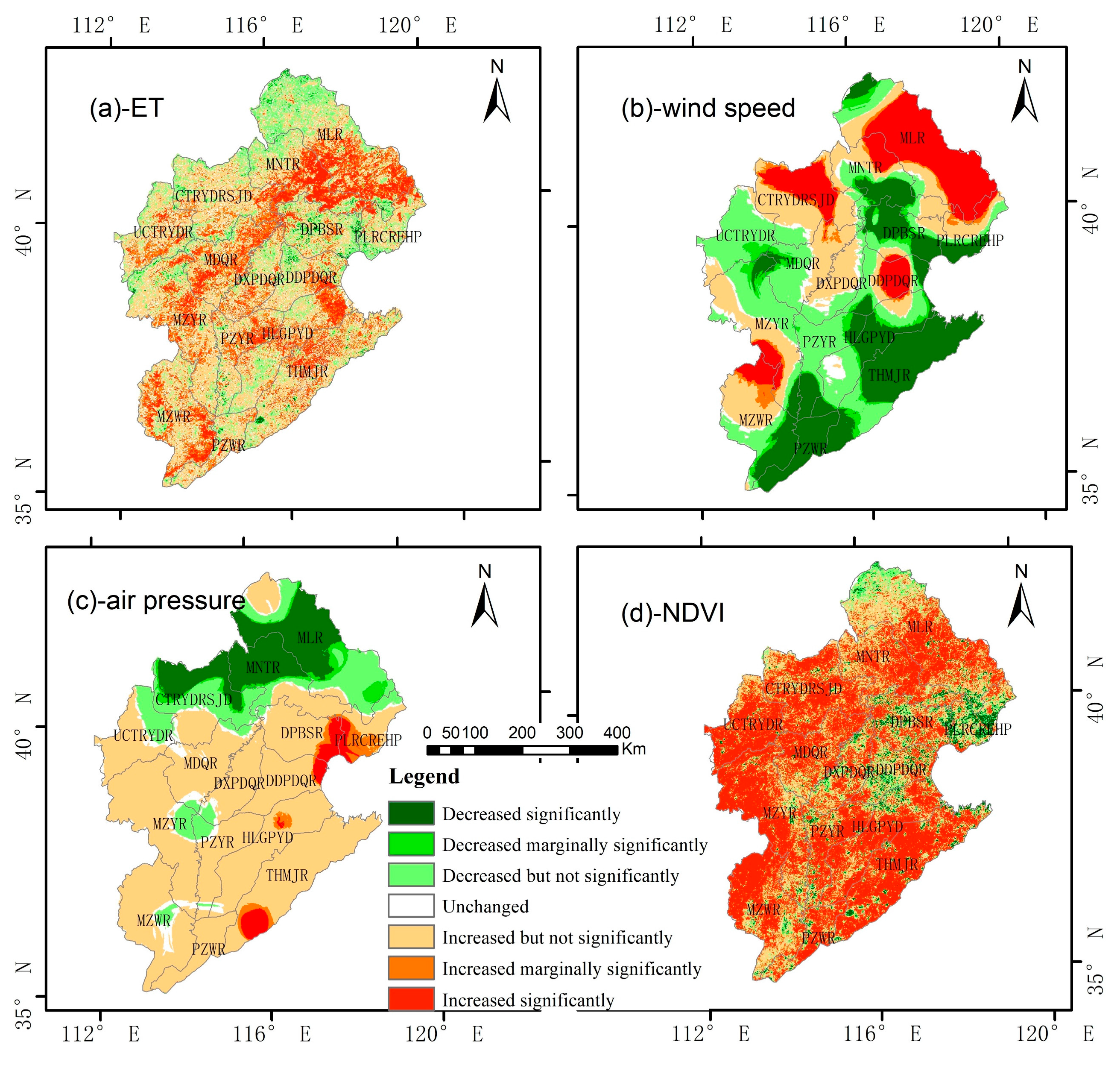
To reveal the temporal trends in the Hai Basin, an M-K test was performed in 1 km × 1 km pixels. Figure 6a–d shows the ET, wind speed, air pressure and NDVI trends in the Hai Basin. ET decreased significantly in the central and eastern portions of DPBSR and increased significantly in southeastern MLR, eastern MNTR and CTRYDRSJD, the majority of MDQR, central MZYR, central HLGPYD and THMJR, eastern HLGPYD and DDPDQR and the majority of MZWR, except the central area. The landscapes of these regions are mainly forest and brush, with some cropland. Most of the Hai Basin experienced a significant increase in the NDVI, except PLRCREHP, western DPBSR, most of DDPQR, northern MLR and lower MZWR. Additionally, the NDVI decreased significantly in western DPBSR and most of DDPQR due to the increase in precipitation and the afforestation policy for barren hills in the Hai Basin [60]. The air pressure decreased significantly in the northern Hai Basin and increased in western DPBSR and eastern PLRCREHP. The wind speed increased significantly in most of MLR, central DDPDQR and northern MZWR but decreased in the southern and southeastern Hai Basin, including most of DPBSR and southern MNTR.
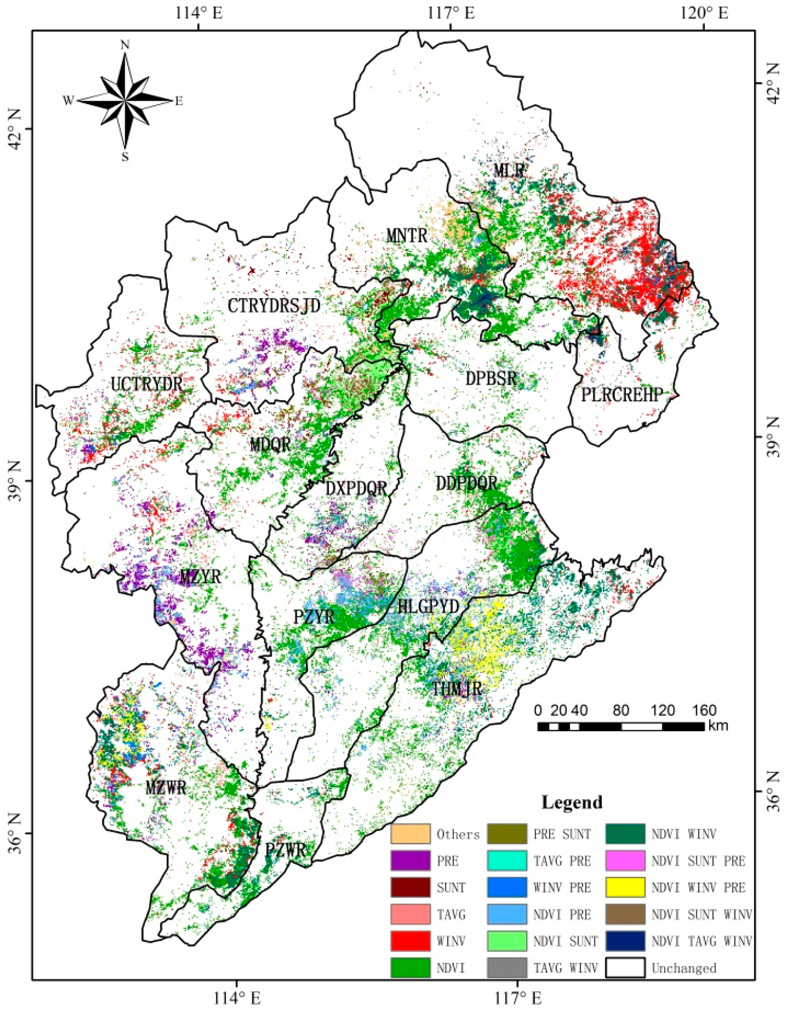
Figure 7 presents the factors that are significantly correlated (Pearson relationship coefficient of R > 0.51) with ET in areas of significant or marginally significant changes in ET from 2000 to 2014. The increase in ET in eastern MLR was related to wind speed, the NDVI and their combination. In eastern MNTR and CTRYDRSJD and the majority of MDQR, many factors were correlated with ET, including the NDVI, wind speed, sunshine hours, air pressure and their combinations. Air pressure was significantly correlated with ET in southern CTRYDRSJD and southwestern MZYR. Additionally, ET was correlated with the NDVI, air pressure, wind speed and their combinations in northeastern PZYR and central HLGPYD and THMJR. In eastern HLGPYD and DDPDQR, the NDVI was the main factor correlated with ET. Three factors are related to ET in MZWR: the NDVI, wind speed, air pressure and their combinations. Most regions were affected by combinations of factors, and only a few were influenced by a single factor. The areas where combinations of the NDVI and the three meteorological parameters (wind speed, sunshine hours or air pressure) were correlated with ET accounted for approximately 74% of the total area of ET change.
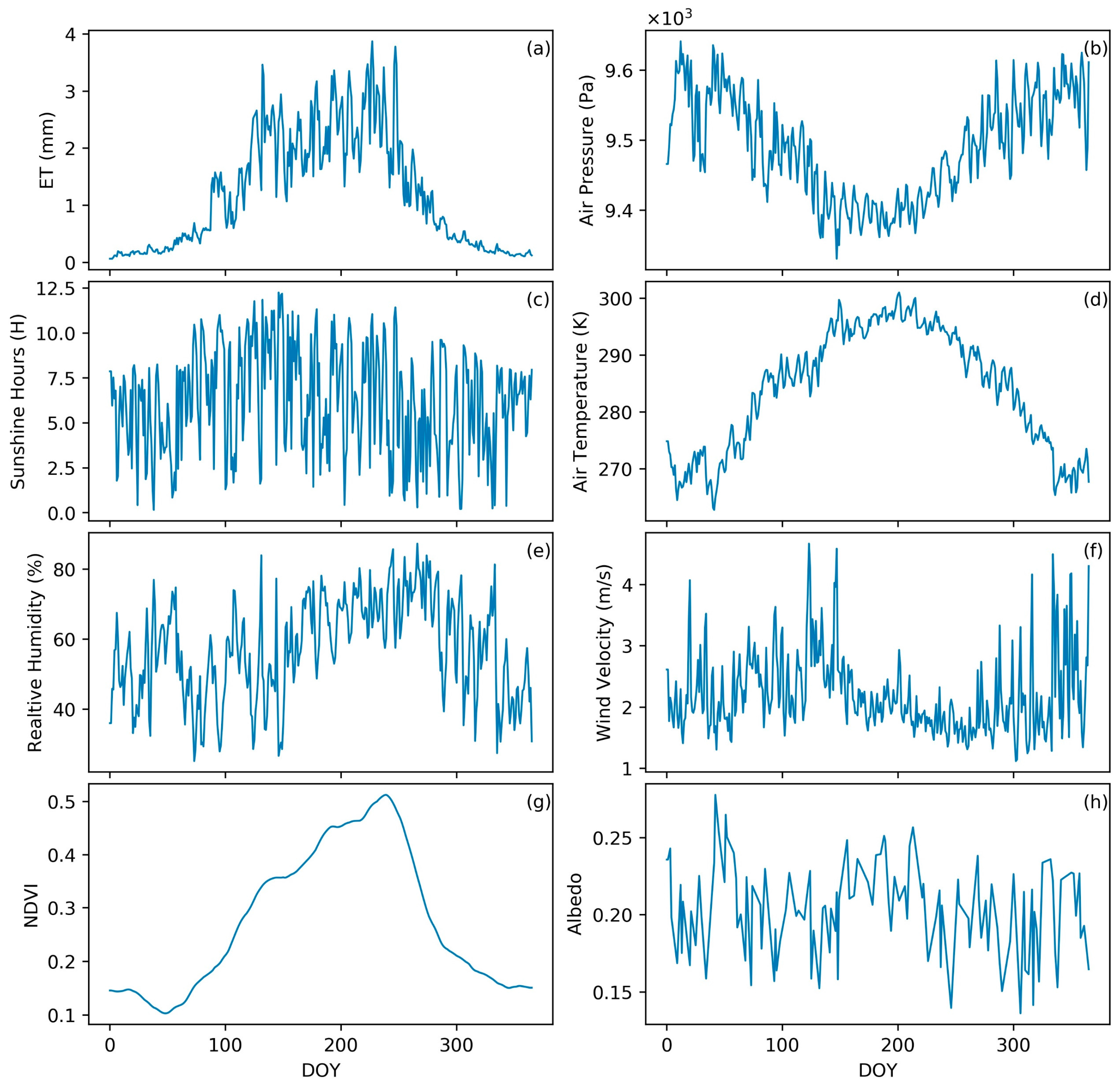
The trends of ET and other parameters are shown in Figure 8. The diurnal average ET in the Hai Basin declined after rising around the 200th day of the year. To locate the times of abrupt changes, M-K abrupt change detection was performed, and the results revealed that the change occurred on the 191st day (July 10th) of the year.
In addition, the temperature and NDVI exhibited the same trend as ET. Similarly, sunshine hours displayed a corresponding trend but with larger fluctuations. However, air pressure exhibited the opposite result as ET, while the albedo, wind speed and relative humidity displayed no significant trends. To investigate the relationships between ET and parameters, the Pearson correlation coefficient developed by Karl Pearson [62] was calculated. The Pearson coefficient is a measure of the linear correlation between two variables. The correlation coefficients between ET and NDVI, air temperature, air pressure, sunshine hours, relative humidity, wind speed and albedo were 0.88, 0.84, −0.79, 0.45, 0.19, −0.02 and −0.01, respectively.
4.3. Quantitative Analysis of the Effects on ET
Both the Mann-Kendall test and t-test were performed to assess the significance of increasing trends exhibited by ET and parameter series, and Table 2 shows the associated results. The major findings are as follows: (i) for ET, albedo, relative humidity, the NDVI, sunshine hours and temperature, significant (p = 0.05) increasing trends were revealed by the Mann-Kendall test and t-test for the entire Hai Basin; (ii) for air pressure, significant (p = 0.05) decreasing trends were observed for the entire Hai Basin; and (iii) for wind speed, no particular trend was found in the Hai Basin.
Detrended analysis was conducted on every pixel for the parameters with significant trends (p = 0.05). Table 3 shows that the difference between the original ET and recalculated ET based on the detrended average air temperature and NDVI were 188.73 mm and 125.35 mm, respectively. The contributions of other factors are small and can be considered negligible. Therefore, the increasing trends in air temperature and NDVI were the main factors for the increase in ET.
5. Discussion
Conclusions regarding ET change at different spatial and temporal scales may be inconsistent. Some previous studies concluded that ET decreased over the past 50 years [26,27], but such findings conflict with the results of this research. This contradiction may result from different spatial scales, and most previous studies were based on meteorological station data. Meteorological stations are generally located in a specific landscape, such as an urban area, grassland or forest. If grassland is converted to forest via the afforestation of barren hills, evapotranspiration will increase by approximately 234.2 mm (Figure 4), which is a larger influence than that associated with climate change. This type of change cannot be reflected in trend analyses based on meteorological station-specific data. Therefore, previous analyses may not reflect the actual changes and trends occurring at the basin scale, especially in the Hai Basin, where the landscape is heterogeneous and land cover has considerably changed over time. Trend analyses based on RS data, which provide detailed information over heterogeneous landscapes at the basin scale, can reliably yield ET changes and trends, including the effects of land cover changes and climate change.
In analyses of interannual temporal changes or one-year trends, the combinations of the NDVI and meteorological parameters were the main factors that affected ET. Climate change, especially precipitation [60] and temperature [63] changes, can affect vegetation cover conditions. The slight increasing trends in temperature and precipitation improved the vegetation cover conditions in the basin. Additionally, the NDVI more rapidly responds to human activities, such as land cover change, than to climate change. Figure 6a shows that most of the areas with significant ET changes were affected by the scope of human activities. Most of these areas were cropland areas, such as those in DDPDQR, DXPDQR, PZYR, HLGPYD, THMJR, PZWR, and DPBSR.
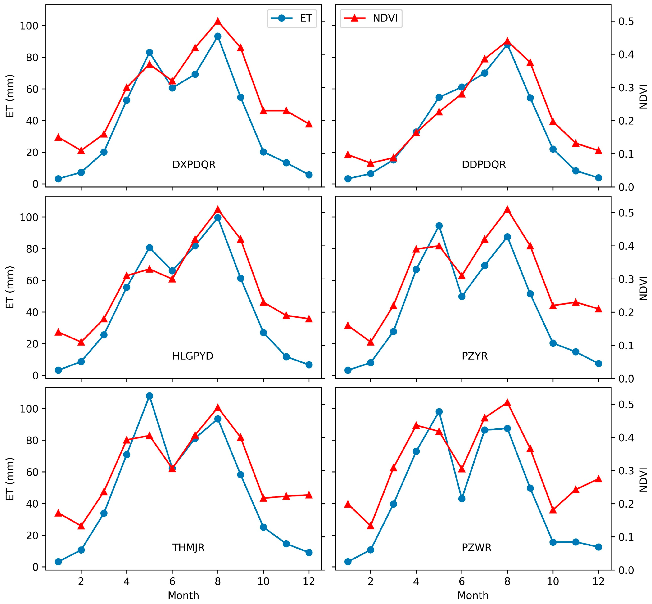
There are the two special regions where the NDVI change was dominant factor for the ET. One is in the area of DDPDQR, DXPDQR, PZYR, HLGPYD, THMJR and PZWR. The cultivated arable land accounted about 90% of the total regions. These regions are major irrigated areas of the North of China Plain, with an average ET of 564.00 mm and precipitation of 531.29 mm, which confirm the predominate effect of human activity. As shown in Figure 9, Evapotranspiration have dual-peak in DDPDQR, DXPDQR, PZYR, HLGPYD, THMJR, PZWR, where exactly is two season crop area with the rotation of winter wheat and summer maize. In DDPDQR, there is only one peak of Evapotranspiration around the year as well as NDVI, where may be the single crop area growing cotton. Therefore, the pattern of ET (single-peak or dual-peak) is determined by NDVI or planting structure in irrigated area.
The other is in the area of MNTR and MLR. Some ecological restoration projects were implemented in this region by the government to improve the living environment in the basin. Such projects include the Grain to Green program and soil conservation projects. These projects expanded the area of vegetation coverage. It is reported that the first stage of construction of ecological water source protection forest were implemented and increased 333.3 km2 of forest in Miyun and Guanting Reservoirs. Zeng et al. analyzed the vegetation fraction change during 2000–2007 and found that the vegetation fraction increased 5% [60]. The increase of ET was mostly attributed to the increase of vegetation fraction. Therefore, the reforestation activities had more impacts on regional water consumption. Although the significant increase in ET is a comprehensive result of climate change and human activities, the effects of human activities may be larger than those of climate change.
The Hai Basin is facing a serious water shortage due to the increase in ET. Fei et al. predicted that the Hai Basin might experience increases in ET and precipitation in the future based on the three-layer variable infiltration capacity (VIC-3 L) model [57,64,65]. In the study period of 2000 to 2014, these changes occurred, but precipitation did not significantly increase (T = 0.79, Z = 0.99) and had a smaller slope (3.00 mm per year) than ET; thus, the volume of available water decreased. If the consumption of water cannot be reduced, the groundwater table will continue to decline, and the water crisis will worsen.
To achieve the goal of sustainable development and solve the issues involving the indiscriminate exploitation of groundwater, a balance must be maintained between available water and water consumption. ET data analysis is one important component that can contribute to assessment of water resources. Two cases were given here. It is reported that the Beijing and Hebei governments will create 5333.6 km2 of water-conserving forest areas near Miyun and Guanting Reservoirs from 2012 to 2020 [66]. Assuming that the increased forest area was converted from grassland, the water consumption would increase 1.36 billion m3, accounting about 21.9% of the volume of water resource deficit (6.23 billion m3) [9], based on the difference (255.3 mm) between forest ET (530.7 mm) and ET (275.4 mm). It is notable that these projects also cause the decrease of outflow and deteriorated water crisis.
The second case involves agricultural conservation projects aimed at saving water and improving the water use efficiency. Agricultural water conservation projects have been launched since the 1980s, including canal lining, mulching, zero tillage, and deficit irrigation measures [10]. In this study, the results show that water consumption in above mentioned several major agricultural areas increased significantly, which suggests that the total water consumption associated with agriculture increased. The implemented water saving measures did not play a role on alleviating the regional water resource utilization issues, and have led to new ecological problems, such as groundwater overexploitation. Therefore, there must be a tradeoff between ecological restoration and other water uses. The sustainable solution is to reduce the total regional agriculture water consumption, mainly relying on reducing the irrigated area. This viewpoint coincides with the conclusion of the study by Wu [9].
6. Conclusions
In this study, spatiotemporal trends of actual ET in the Hai Basin and the associated factors were analyzed. The M-K nonparametric test was employed to reveal the interannual and annual ET trends, while a spatial analysis in GIS was used to explore the spatial distributions of parameters in the Hai Basin. Based on detrended analysis and Pearson correlation coefficients, the effects of these parameters on ET were quantified. The main conclusions are as follows.
ET increased from northwest to southeast. When the landscape was taken into account, the ET of water was highest, followed by those of paddy fields, forest, cropland, brush and grassland areas, while settlement had the lowest ET. The ET-based water consumption of cropland accounted for approximately 50.1% of consumption, followed by forest areas at 22.4%, brush at 11.9%, grassland at 7.8% and other landscapes at 7.8%.
From 2000 to 2014, ET increased by approximately 3.70 mm per year in the Hai Basin, which is a comprehensive result of climate change and human activities. Spatially, ET increased significantly in the southeastern MLR; eastern MNTR, HLGPYD, DDPDQR and CTRYDRSJD; most of MDQR, central MZYR, HLGPYD, and THMJR; and most of MZWR, except the central area. The majority of the Hai Basin exhibited a significant increase in NDVI. This result suggested that agricultural water conservation projects implemented over the past fifteen years did play an effective role in reducing water consumption at the regional scale. The basin will likely face increasingly serious water resource issues if the increasing ET trend cannot be reversed or mitigated.
The causal analysis showed that the NDIV, wind speed, and air pressure were three main factors highly correlated with annual ET. Most regions were affected by combinations of factors, and only a few were affected by a single factor. The areas where combinations of the NDVI and the three meteorological parameters (wind speed, sunshine hours or air pressure) were correlated with ET accounted for approximately 74% of the total area of ET change.
ET increased from the 1st to 191st days of the year and decreased after the major shift on 10 July. Temperature and the NDVI were the main causes of the increasing trend in ET between days 1 and 191 of the year. Because the temperature and NDVI largely explained the increasing trend in ET in 2014, they can be used as indicators to evaluate ET and provide early warning for associated issues. Notably, the NDVI accounted for 57.16% of the ET at the annual scale.
Acknowledgments
This study was supported financially by National Natural Science Foundation of China (No. 41601463, 41701403) and Key Research Program of Frontier Science, CAS (Grant No. QYZDY-SSW-DQC014).
Author Contributions
Nana Yan conceived this research and was responsible for the research. Fuyou Tian contributed to process and analyze data, and wrote the paper. Bingfang Wu warrant ETWatch model to calculate ET in Hai Basin. Weiwei Zhu calculated ET in Hai Basin. Mingzhao Yu collected and preprocessed the original data. All the co-authors helped to polish the manuscript.
Conflicts of Interest
The authors declare no conflict of interest.
References
- Hu, G.; Jia, L.; Menenti, M. Comparison of MOD16 and LSA-SAF MSG evapotranspiration products over europe for 2011. Remote Sens. Environ. 2015, 156, 510–526. [Google Scholar] [CrossRef]
- Mao, Y.; Wang, K.; Liu, X.; Liu, C. Water storage in reservoirs built from 1997 to 2014 significantly altered the calculated evapotranspiration trends over China. J. Geophys. Res. Atmos. 2016, 121, 10097–10112. [Google Scholar] [CrossRef]
- Sheffield, J.; Wood, E.F.; Munoz-Arriola, F. Long-term regional estimates of evapotranspiration for mexico based on downscaled isccp data. J. Hydrometeorol. 2010, 11, 253–275. [Google Scholar] [CrossRef]
- Rivas, R.; Caselles, V. A simplified equation to estimate spatial reference evaporation from remote sensing-based surface temperature and local meteorological data. Remote Sens. Environ. 2004, 93, 68–76. [Google Scholar] [CrossRef]
- Jin, Y.; Randerson, J.T.; Goulden, M.L. Continental-scale net radiation and evapotranspiration estimated using modis satellite observations. Remote Sens. Environ. 2011, 115, 2302–2319. [Google Scholar] [CrossRef]
- Baumgartner, A.; Reichel, E. The World Water Balance: Mean Annual Global, Continental and Maritime Precipitation and Run-Off; Elsevier: Amsterdam, The Netherlands, 1975; p. 1975. [Google Scholar]
- Xu, Z.; Yang, H.-B.; Liu, F.-D.; An, S.-Q.; Cui, J.; Wang, Z.-S.; Liu, S.-R. Partitioning evapotranspiration flux components in a subalpine shrubland based on stable isotopic measurements. Bot. Stud. 2008, 49, 351–361. [Google Scholar]
- Allen, R.G.; Pereira, L.S.; Raes, D.; Smith, M. Crop evapotranspiration-guidelines for computing crop water requirements-fao irrigation and drainage paper 56. FAO Rome 1998, 300, D05109. [Google Scholar]
- Wu, B.; Jiang, L.; Yan, N.; Perry, C.; Zeng, H. Basin-wide evapotranspiration management: Concept and practical application in Hai Basin, China. Agric. Water Manag. 2014, 145, 145–153. [Google Scholar] [CrossRef]
- Yan, N.; Wu, B.; Perry, C.; Zeng, H. Assessing potential water savings in agriculture on the Hai Basin plain, China. Agric. Water Manag. 2015, 154, 11–19. [Google Scholar] [CrossRef]
- Liu, Q.; Yang, Z. Quantitative estimation of the impact of climate change on actual evapotranspiration in the Yellow River Basin, China. J. Hydrol. 2010, 395, 226–234. [Google Scholar] [CrossRef]
- Yang, Y.; Yang, Y.; Liu, D.; Nordblom, T.; Wu, B.; Yan, N. Regional water balance based on remotely sensed evapotranspiration and irrigation: An assessment of the Haihe plain, China. Remote Sens. 2014, 6, 2514–2533. [Google Scholar] [CrossRef]
- Wang, K.; Dickinson, R. A review of global terrestrial evapotranspiration: Observation, modeling, climatology, and climatic variability. Rev. Geophys. 2012, 50. [Google Scholar] [CrossRef]
- Kosugi, Y.; Katsuyama, M. Evapotranspiration over a japanese cypress forest. Ii. Comparison of the eddy covariance and water budget methods. J. Hydrol. 2007, 334, 305–311. [Google Scholar] [CrossRef]
- Wilson, K.B.; Hanson, P.J.; Mulholland, P.J.; Baldocchi, D.D.; Wullschleger, S.D. A comparison of methods for determining forest evapotranspiration and its components: Sap-flow, soil water budget, eddy covariance and catchment water balance. Agric. For. Meteorol. 2001, 106, 153–168. [Google Scholar] [CrossRef]
- Liu, C.; Zhang, X.; Zhang, Y. Determination of daily evaporation and evapotranspiration of winter wheat and maize by large-scale weighing lysimeter and micro-lysimeter. Agric. For. Meteorol. 2002, 111, 109–120. [Google Scholar] [CrossRef]
- Nagler, P.L.; Scott, R.L.; Westenburg, C.; Cleverly, J.R.; Glenn, E.P.; Huete, A.R. Evapotranspiration on western us rivers estimated using the enhanced vegetation index from modis and data from eddy covariance and bowen ratio flux towers. Remote Sens. Environ. 2005, 97, 337–351. [Google Scholar] [CrossRef]
- Wu, B.; Yan, N.; Xiong, J.; Bastiaanssen, W.G.M.; Zhu, W.; Stein, A. Validation of etwatch using field measurements at diverse landscapes: A case study in Hai Basin of China. J. Hydrol. 2012, 436–437, 67–80. [Google Scholar] [CrossRef]
- Bastiaanssen, W.G.M.; Menenti, M.; Feddes, R.A.; Holtslag, A.A.M. A remote sensing surface energy balance algorithm for land (SEBAL). 1. Formulation. J. Hydrol. 1998, 212–213, 198–212. [Google Scholar] [CrossRef]
- Cleugh, H.A.; Leuning, R.; Mu, Q.; Running, S.W. Regional evaporation estimates from flux tower and modis satellite data. Remote Sens. Environ. 2007, 106, 285–304. [Google Scholar] [CrossRef]
- Su, Z. The surface energy balance system (SEBS) for estimation of turbulent heat fluxes. Hydrol. Earth Syst. Sci. Discuss. 2002, 6, 85–100. [Google Scholar] [CrossRef]
- Wu, B.; Xiong, J.; Yan, N.; Yang, L. Etwatch: An Operational et Monitoring System with Remote Sensing. In Proceedings of the 2008 ISPRS Workshop on Geo-Information and Decision Support Systems, Tehran, Iran, 6–7 January 2008. [Google Scholar]
- Bastiaanssen, W.G.M.; Pelgrum, H.; Wang, J.; Ma, Y.; Moreno, J.F.; Roerink, G.J.; van der Wal, T. A remote sensing surface energy balance algorithm for land (SEBAL): Part 2: Validation. J. Hydrol. 1998, 212–213, 213–229. [Google Scholar] [CrossRef]
- Mu, Q.; Zhao, M.; Running, S.W. Improvements to a MODIS global terrestrial evapotranspiration algorithm. Remote. Sens. Environ. 2011, 115, 1781–1800. [Google Scholar] [CrossRef]
- Monteith, J. Evaporation and environment. Symp. Soc. Exp. Biol. 1965, 19, 4. [Google Scholar]
- Li, X.; Gemmer, M.; Zhai, J.; Liu, X.; Su, B.; Wang, Y. Spatio-temporal variation of actual evapotranspiration in the haihe river basin of the past 50 years. Quat. Int. 2013, 304, 133–141. [Google Scholar] [CrossRef]
- Lu, S.; Wu, B.; Wei, Y.; Yan, N.; Wang, H.; Guo, S. Quantifying impacts of climate variability and human activities on the hydrological system of the Haihe River Basin, China. Environ. Earth Sci. 2015, 73, 1491–1503. [Google Scholar] [CrossRef]
- Liu, M.; Tian, H.; Chen, G.; Ren, W.; Zhang, C.; Liu, J. Effects of land-use and land-cover change on evapotranspiration and water yield in China during 1900–2000. JAWRA J. Am. Water Resour. Assoc. 2008, 44, 1193–1207. [Google Scholar] [CrossRef]
- Hu, Y.; Moiwo, J.P.; Yang, Y.; Han, S.; Yang, Y. Agricultural water-saving and sustainable groundwater management in Shijiazhuang Irrigation District, North China Plain. J. Hydrol. 2010, 393, 219–232. [Google Scholar] [CrossRef]
- Xu, C.-Y.; Gong, L.; Jiang, T.; Chen, D.; Singh, V.P. Analysis of spatial distribution and temporal trend of reference evapotranspiration and pan evaporation in Changjiang (Yangtze River) catchment. J. Hydrol. 2006, 327, 81–93. [Google Scholar] [CrossRef]
- Li, Z.; Zhang, Y.-K. Quantifying fractal dynamics of groundwater systems with detrended fluctuation analysis. J. Hydrol. 2007, 336, 139–146. [Google Scholar] [CrossRef]
- Zhang, Q.; Xu, C.-Y.; Chen, Y.D.; Yu, Z. Multifractal detrended fluctuation analysis of streamflow series of the Yangtze River Basin, China. Hydrol. Process. 2008, 22, 4997–5003. [Google Scholar] [CrossRef]
- Zhang, Q.; Zhou, Y.; Singh, V.P.; Chen, Y.D. Comparison of detrending methods for fluctuation analysis in hydrology. J. Hydrol. 2011, 400, 121–132. [Google Scholar] [CrossRef]
- Tegos, A.; Malamos, N.; Efstratiadis, A.; Tsoukalas, I.; Karanasios, A.; Koutsoyiannis, D. Parametric modelling of potential evapotranspiration: A global survey. Water 2017, 9, 795. [Google Scholar] [CrossRef]
- Zhao, M.; Cheng, W.; Liu, Q.; Wang, N. Spatiotemporal measurement of urbanization levels based on multiscale units: A case study of the Bohai Rim Region in China. J. Geogr. Sci. 2016, 26, 531–548. [Google Scholar] [CrossRef]
- Kuang, W.; Liu, J.; Zhang, Z.; Lu, D.; Xiang, B. Spatiotemporal dynamics of impervious surface areas across china during the early 21st century. Chin. Sci. Bull. 2013, 58, 1691–1701. [Google Scholar] [CrossRef]
- Wu, B.; Yuan, Q.; Yan, C.; Wang, Z.; Yu, X.; Li, A.; Ma, R.H.; Huang, J.L.; Chen, J.S.; Chang, C. Land cover changes of China from 2000 to 2010. Quat. Sci. 2014, 34, 723–731. [Google Scholar]
- Guo, Y.; Shen, Y. Quantifying water and energy budgets and the impacts of climatic and human factors in the Haihe River Basin, China: 2. Trends and implications to water resources. J. Hydrol. 2015, 527, 251–261. [Google Scholar] [CrossRef]
- Changming, L.; Jingjie, Y.; Kendy, E. Groundwater exploitation and its impact on the environment in the North China Plain. Water Int. 2001, 26, 265–272. [Google Scholar] [CrossRef]
- Laads Web: Level-1 and Atmosphere Archive & Distribution System. Available online: https://ladsweb.modaps.eosdis.nasa.gov/search/ (accessed on 24 August 2017).
- LAADS DAAC. Mod021km-Level 1b Calibrated Radiances-1km. Available online: https://ladsweb.modaps.eosdis.nasa.gov/api/v1/productPage/product=MOD021KM (accessed on 12 December 2017).
- Vermote, E.F.; Tanré, D.; Deuze, J.L.; Herman, M.; Morcette, J.J. Second simulation of the satellite signal in the solar spectrum, 6s: An overview. IEEE Trans. Geosci. Remote Sens. 1997, 35, 675–686. [Google Scholar] [CrossRef]
- Li, Z.-L.; Tang, B.-H.; Wu, H.; Ren, H.; Yan, G.; Wan, Z.; Trigo, I.F.; Sobrino, J.A. Satellite-derived land surface temperature: Current status and perspectives. Remote Sens. Environ. 2013, 131, 14–37. [Google Scholar] [CrossRef]
- Mao, K.; Qin, Z.; Shi, J.; Gong, P. A practical split-window algorithm for retrieving land-surface temperature from modis data. Int. J. Remote Sens. 2005, 26, 3181–3204. [Google Scholar] [CrossRef]
- Qian, Q.; Wu, B.; Xiong, J. Interpolation system for generating meteorological surfaces using to compute evapotranspiration in Haihe River Basin. In Proceedings of the 2005 IEEE International Geoscience and Remote Sensing Symposium, Seoul, Korea, 29 July 2005. [Google Scholar]
- Yan, N.; Zhu, W.; Feng, X.; Chang, S. Spatial-temporal change analysis of evapotranspiration in the Heihe River Basin. In Proceedings of the 2014 Third International Workshop on Earth Observation and Remote Sensing Applications (EORSA), Changsha, China, 11–14 June 2014; pp. 38–41. [Google Scholar]
- Zhang, L.; Li, X.; Yuan, Q.; Liu, Y. Object-based approach to national land cover mapping using HJ satellite imagery. J. Appl. Remote Sens. 2014, 8, 083686. [Google Scholar] [CrossRef]
- Birsan, M.-V.; Molnar, P.; Burlando, P.; Pfaundler, M. Streamflow trends in Switzerland. J. Hydrol. 2005, 314, 312–329. [Google Scholar] [CrossRef]
- Sprent, P.; Smeeton, N.C. Applied Nonparametric Statistical Methods; CRC Press: Boca Raton, FL, USA, 2007. [Google Scholar]
- Box, J.F. Guinness, gosset, fisher, and small samples. Stat. Sci. 1987, 2, 45–52. [Google Scholar] [CrossRef]
- Kendall, M.G. A new measure of rank correlation. Biometrika 1938, 30, 81–93. [Google Scholar] [CrossRef]
- Gibbons, J.D.; Chakraborti, S. Nonparametric Statistical Inference; Springer: Berlin, Germany, 2011. [Google Scholar]
- De la Casa, A.C.; Ovando, G.G. Variation of reference evapotranspiration in the central region of Argentina between 1941 and 2010. J. Hydrol. Reg. Stud. 2016, 5, 66–79. [Google Scholar] [CrossRef]
- Douglas, E.M.; Vogel, R.M.; Kroll, C.N. Trends in floods and low flows in the United States: Impact of spatial correlation. J. Hydrol. 2000, 240, 90–105. [Google Scholar] [CrossRef]
- Bao, Z.; Zhang, J.; Wang, G.; Fu, G.; He, R.; Yan, X.; Jin, J.; Liu, Y.; Zhang, A. Attribution for decreasing streamflow of the Haihe River Basin, Northern China: Climate variability or human activities? J. Hydrol. 2012, 460, 117–129. [Google Scholar] [CrossRef]
- Estes, A.B.; Kuemmerle, T.; Kushnir, H.; Radeloff, V.C.; Shugart, H.H. Land-cover change and human population trends in the greater serengeti ecosystem from 1984–2003. Biol. Conserv. 2012, 147, 255–263. [Google Scholar] [CrossRef]
- Yuan, F.; Xie, Z.H.; Liu, Q.; Xia, J. Simulating hydrologic changes with climate change scenarios in the haihe river basin. Pedosphere 2005, 15, 595–600. [Google Scholar]
- Duo, A.; Zhao, W.; Qu, X.; Jing, R.; Xiong, K. Spatio-temporal variation of vegetation coverage and its response to climate change in North China plain in the last 33 years. Int. J. Appl. Earth Obs. Geoinf. 2016, 53, 103–117. [Google Scholar]
- Xu, G.; Zhang, H.; Chen, B.; Zhang, H.; Innes, J.; Wang, G.; Yan, J.; Zheng, Y.; Zhu, Z.; Myneni, R. Changes in vegetation growth dynamics and relations with climate over China’s landmass from 1982 to 2011. Remote Sens. 2014, 6, 3263–3283. [Google Scholar] [CrossRef]
- Wu, Y.; Zeng, Y.; Zhao, Y.; Wu, B.; Wu, W. Monitoring and dynamic analysis of fractional vegetation cover in the Hai River Basin based on MODIS data. Resour. Sci. 2010, 32, 1417–1424. [Google Scholar]
- Rahman, N.; Macpherson, A.; Rosemblatt, K.A.N. A course in theoretical statistics: For sixth forms, Technical Colleges, Colleges of Education, Universities: Charles Griffin & Company Limited; Charles Griffin & Company Limited: London, UK, 1968. [Google Scholar]
- Pearson, K. Note on regression and inheritance in the case of two parents. Proc. R. Soc. Lond. 1895, 58, 240–242. [Google Scholar] [CrossRef]
- Zhao, M.; Running, S.W. Drought-induced reduction in global terrestrial net primary production from 2000 through 2009. Science 2010, 329, 940–943. [Google Scholar] [CrossRef] [PubMed]
- Liang, X.; Xie, Z. A new surface runoff parameterization with subgrid-scale soil heterogeneity for land surface models. Adv. Water Resour. 2001, 24, 1173–1193. [Google Scholar] [CrossRef]
- Zhenghui, X.; Fengge, S.; Xu, L.; Qingcun, Z.; Zhenchun, H.; Yufu, G. Applications of a surface runoff model with horton and dunne runoff for vic. Adv. Atmos. Sci. 2003, 20, 165–172. [Google Scholar] [CrossRef]
- People.cn. Available online: http://bj.people.com.cn/n/2015/0528/c82840-25035935.html (accessed on 3 September 2017).
Figure 1.
Location of Hai Basin, its subbasins, meteorological stations, and elevation.

Figure 2.
Flowchart of the key procedures embedded in ETWatch [22].
Figure 2.
Flowchart of the key procedures embedded in ETWatch [22].

Figure 3.
The distributions of land use (a) and evapotranspiration (b) and the spatial trend of ET (c) in 2014 in the Hai Basin. The units of evapotranspiration shown in (b) are mm. (c) was created using the ArcGIS trend analysis tool.
Figure 3.
The distributions of land use (a) and evapotranspiration (b) and the spatial trend of ET (c) in 2014 in the Hai Basin. The units of evapotranspiration shown in (b) are mm. (c) was created using the ArcGIS trend analysis tool.

Figure 4.
The area of land use and annual average ET in 2014 in the Hai Basin.

Figure 5.
The trends of ET, precipitation and water surplus from 2000 to 2014 in the Hai Basin.

Figure 6.
The temporal trends of ET (a); wind speed (b); air pressure (c) and NDVI (d) in the Hai Basin during 2000 to 2014. Mann-Kendall test was used in each pixel to determine the trend. Based on the sign of Z, the trends was divided into three: increase: Z > 0, unchanged Z = 0, decrease Z < 0; The confidence were classified into three levels according to absolute value and : significant (), marginally significant () and not significant ().

Figure 7.
Factors (NDVI, air pressure, sunshine time, wind speed, relative humidity and average air temperature) that are significantly correlated (Pearson relationship coefficient of R > 0.51) with ET in areas of significant or marginally significant changes in ET from 2000 to 2014. Assuming that ET and all factors have bivariate normal distributions, the variable has a Student’s t distribution [61]. Factors are significantly correlated with ET when R > 0.51 (T > ).

Figure 8.
The trends in diurnal average ET (a) and parameters (b–h) in 2014, where (b) is the trend of air pressure; (c) is sunshine hours (Sunt); (d) is the average air temperature (Tavg) estimated based on the average of the maximum and minimum; (e) is the relative humidity (Humd); (f) is wind speed (Winv); (g) is the NDVI and (h) is Albedo.

Figure 9.
The variation of average ET and NDVI in DDPDQR, DXPDQR, PZYR, HLGPYD, THMJR, PZWR.


Table 1.
Tests of ET, water surplus and precipitation trends from 2000 to 2014.
| Variable | t-Test | Mann-Kendall Test | ||||||
|---|---|---|---|---|---|---|---|---|
| Slope | T | Tc | H0 | Kendall’s Tau | Z | Zc | H0 | |
| ET * | 3.70 | 2.28 | 2.16 | R | 0.43 | 2.18 | 1.96 | R |
| Precipitation | 3.00 | 0.79 | 2.16 | N.R. | 0.20 | 0.99 | 1.96 | N.R. |
| Water surplus | −0.65 | −0.21 | 2.16 | N.R. | −0.01 | 0.00 | 1.96 | N.R. |
| NDVI * | 0.002 | 5.26 | 2.16 | R | 0.66 | 3.40 | 1.96 | R |
| HUMD | −0.04 | −0.30 | 2.16 | N.R. | −0.09 | −0.40 | 1.96 | N.R. |
| PRE | 0.37 | 0.55 | 2.16 | N.R. | 0.09 | 0.40 | 1.96 | N.R. |
| SUNT | −0.08 | −0.32 | 2.16 | N.R. | −0.12 | −0.59 | 1.96 | N.R. |
| Tavg | 0.07 | 0.19 | 2.16 | N.R. | −0.03 | −0.10 | 1.96 | N.R. |
| Winv | −0.04 | −0.59 | 2.16 | N.R. | −0.18 | −0.89 | 1.96 | N.R. |
Note—H0: no trend; R, rejected; N.R., not rejected; Tc = ; Zc = at the significance level; and * denotes variables that changed significantly.
Table 2.
Trend tests for ET and other parameters.
| Variable | t-Test | Mann-Kendall Test | ||||||
|---|---|---|---|---|---|---|---|---|
| Slope | T | Tc | H0 | Kendall’s Tau | Z | Zc | H0 | |
| ET * | 0.01 | 24.48 | 1.97 | R | 0.75 | 15.50 | 1.96 | R |
| Albedo * | 9.4 × 10⁻⁵ | 2.84 | 1.97 | R | 0.18 | 3.63 | 1.96 | R |
| Relative humidity * | 0.05 | 3.25 | 1.97 | R | 0.16 | 3.22 | 1.96 | R |
| NDVI * | 1.9 × 10⁻³ | 38.74 | 1.97 | R | 0.80 | 16.45 | 1.96 | R |
| Air pressure * | −1.17 | −20.66 | 1.97 | R | −0.63 | −12.98 | 1.96 | R |
| Sunshine hours * | 0.13 | 3.43 | 1.97 | R | 0.17 | 3.60 | 1.96 | R |
| Temperature * | 0.18 | 33.06 | 1.97 | R | 0.74 | 15.17 | 1.96 | R |
| Wind speed | 0.01 | 1.78 | 1.97 | N.R. | 0.08 | 1.73 | 1.96 | N.R. |
Note—H0: no trend; R, rejected; N.R., not rejected; Tc = ; Zc = at the significance level; and * denotes variables that changed significantly.
Table 3.
The difference between original ET and recalculated ET based on detrended parameters series from the 1st to 191st day of 2014 in the Hai Basin, China.
Table 3.
The difference between original ET and recalculated ET based on detrended parameters series from the 1st to 191st day of 2014 in the Hai Basin, China.
| Variable | ET (Original) (mm) | ET (Detrended) (mm) | Difference (mm) |
|---|---|---|---|
| Albedo | 219.31 | 229.38 | −10.08 |
| HUMD | 219.31 | 219.29 | 0.02 |
| NDVI | 219.31 | 93.95 | 125.35 |
| PRE | 219.31 | 234.15 | −14.84 |
| SUNT | 219.31 | 202.01 | 17.29 |
| Tavg | 219.31 | 30.58 | 188.73 |
© 2018 by the authors. Licensee MDPI, Basel, Switzerland. This article is an open access article distributed under the terms and conditions of the Creative Commons Attribution (CC BY) license (http://creativecommons.org/licenses/by/4.0/).
Share and Cite
MDPI and ACS Style
Yan, N.; Tian, F.; Wu, B.; Zhu, W.; Yu, M. Spatiotemporal Analysis of Actual Evapotranspiration and Its Causes in the Hai Basin. Remote Sens. 2018, 10, 332. https://doi.org/10.3390/rs10020332
AMA Style
Yan N, Tian F, Wu B, Zhu W, Yu M. Spatiotemporal Analysis of Actual Evapotranspiration and Its Causes in the Hai Basin. Remote Sensing. 2018; 10(2):332. https://doi.org/10.3390/rs10020332
Chicago/Turabian StyleYan, Nana, Fuyou Tian, Bingfang Wu, Weiwei Zhu, and Mingzhao Yu. 2018. "Spatiotemporal Analysis of Actual Evapotranspiration and Its Causes in the Hai Basin" Remote Sensing 10, no. 2: 332. https://doi.org/10.3390/rs10020332
Note that from the first issue of 2016, this journal uses article numbers instead of page numbers. See further details here.