Geostationary Visible Imager Calibration for the CERES SYN1deg Edition 4 Product

1
NASA Langley Research Center, Hampton, VA 23681, USA
2
Science Systems and Applications, Inc., 1 Enterprise Pkwy, Hampton, VA 23666, USA
*
Author to whom correspondence should be addressed.
Remote Sens. 2018, 10(2), 288; https://doi.org/10.3390/rs10020288
Submission received: 10 January 2018
/
Revised: 7 February 2018
/
Accepted: 8 February 2018
/
Published: 13 February 2018
(This article belongs to the Section Atmospheric Remote Sensing)
Abstract
:The Clouds and the Earth’s Radiant Energy System (CERES) project relies on geostationary (GEO) imager derived TOA broadband fluxes and cloud properties to account for the regional diurnal fluctuations between the Terra and Aqua CERES and MODIS measurements. Anchoring the GEO visible calibration to the MODIS reference calibration and stability is critical for consistent fluxes and cloud retrievals across the 16 GEO imagers utilized in the CERES record. The CERES Edition 4A used GEO and MODIS ray-matched radiance pairs over all-sky tropical ocean (ATO-RM) to transfer the MODIS calibration to the GEO imagers. The primary GEO ATO-RM calibration was compared with the deep convective cloud (DCC) ray-matching and invariant desert/DCC target calibration methodologies, which are all tied to the same Aqua-MODIS calibration reference. Results indicate that most GEO record mean calibration method biases are within 1% with respect to ATO-RM. Most calibration method temporal trends were within 0.5% relative to ATO-RM. The monthly gain trend standard errors were mostly within 1% for all methods and GEOs. The close agreement amongst the independent calibration techniques validates all methodologies, and verifies that the coefficients are not artifacts of the methodology but rather adequately represent the true GEO visible imager degradation.

1. Introduction
The Clouds and the Earth’s Radiant Energy System CERES project [1] synoptic gridded (SYN1deg) product relies on geostationary visible imager (GEO) derived TOA broadband fluxes and retrieved cloud properties to account for the regional diurnal fluctuations from times between the CERES and Moderate Resolution Imaging Spectroradiometer (MODIS) measurement intervals [2]. The MODIS and GEO cloud properties are used to compute the hourly surface fluxes contained in the SYN1deg product [3]. The GEO cloud properties are used to select the appropriate surface/cloud conditions, referred to as scene types, for the GEO visible radiance to broadband flux conversion algorithm. The GEO-derived TOA SW fluxes are radiometrically scaled regionally to the CERES SW fluxes to maintain the CERES instrument calibration in the CERES SYN1deg product. The scaling also removes any outstanding GEO derived flux artifacts as a result of inadequate calibration, cloud properties, narrowband to broadband models, or angular distribution models.
To achieve uniformity in cloud properties and computed surface fluxes across the GEO domains in both time and space, each of the 16 GEOs in the CERES record must be inter-calibrated using the same calibration reference. Except for Himawari-8, the GEOs do not have onboard visible calibration systems, and therefore instrument gains must be externally adjusted for both the absolute calibration and the calibration temporal stability. Cloud properties from the GEOs and MODIS are incorporated in the SYN1deg product, which means cloud property consistency between the instruments is crucial. CERES Edition 3A (Ed3A) used Terra-MODIS Collection 5 (C5) band 1 (0.65 µm) as the visible reference. Terra-MODIS C5 band 1 has a calibration trend of −1.6% to −2.5% between 2000 and 2011, based on invariant Earth targets [4]. For Aqua-MODIS C6 band 1, the trend drifted between 0.0% and −1.4%, with most of the drift occurring after 2008 [5]—a clear improvement in stability over the Terra-MODIS C5 band 1 record. The Aqua-MODIS degradation is mostly due to response versus scan-angle (RVS) issues [6]. The CERES Edition 4A (Ed4A) GEO calibration uses Aqua-MODIS C6 band 1 as a reference and follows the recommendation of the Global Spaced-based Inter-Calibration System (GSICS) [7] as it exceeds the performance of Terra-MODIS [8,9].
Figure 1 displays the 16 geostationary satellites (GEOsats) utilized during the CERES Terra and Aqua record. For a real-time GEO record time line, consult the CERES project website [10]. The GEOsats include: Met-5 and Met-7 Meteosat First Generation (MFG) Meteosat Visible and Infrared Imager (MVIRI) [11]; Met-8–10, Meteosat Second Generation (MSG) Spinning Enhanced Visible and Infrared Imagers (SEVIRI) [12]; the GMS-5 Geostationary Meteorological Satellite (GMS) Visible and Infrared Spin Scan Radiometer (VISSR) [13]; MTSAT-1R Multifunctional Transport Satellites (MTSAT) Japanese Advanced Meteorological Imager (JAMI) [14]; MTSAT-2 imager, Himwari-8 Advanced Himawari Imager (AHI) [15]; and GOES-8–15 Geostationary Operational Environmental Satellite (GOES) imagers [16]. All operational GEOsat outages, and the associated backup GEOsats employed, are documented. Major outages were due to deicing events for Meteosat-10 [17,18], annual ground maintenance periods for MTSAT-2 [19,20] which typically occurs for a month near the end of a calendar year, and two unknown events for GOES-13 [21,22], for which GOES-14 was operational from 24 September to 17 October 2012, and 23 May to 9 June 2013. For Ed4A, the GEO imagery was first inspected for spurious scan lines. An automated bad scan line detection algorithm was designed to identify almost all GEO linear artifacts [23]. All flagged GEO imagery was then examined visually, in which the linear artifacts were verified and removed from the image, while leaving algorithm false positives intact. The 1st-generation GEO cloud properties were based on the same Ed3A 2-channel cloud retrieval code [24]. The 2nd and 3rd generation GEOsats use a multiple-channel cloud retrieval code that is designed to retrieve MODIS-quality cloud properties. Hourly GEO data are ingested for CERES SYN1deg Ed4A product, whereas for Ed3A the GEO temporal resolution was 3-hourly.
This article describes the CERES Ed4A GEO visible imager calibration approach. The paper is organized as follows. The multiple CERES GEO calibration methodologies are described in Section 2. Section 3 compares the multiple calibration approaches to assess the consistency in terms of both the absolute calibration with respect to MODIS and trend stability. Section 4 provides the CERES Ed4A GEO calibration coefficients and their associated uncertainties. Discussion and conclusions are found in Section 5 and 6, respectively.
2. Methodology
The CERES Ed4A GEO visible imager calibration relies on all-sky tropical ocean ray-matching (ATO-RM) as the primary calibration method to transfer the Aqua-MODIS C6 band 1 (0.65 µm) reference calibration to GEO. The ATO-RM method uses coincident co-angled, and co-located MODIS and GEO instantaneous radiance/count pairs acquired over a predefined domain centered at the GEO sub-satellite point. The ray-matched MODIS radiances and GEO counts are regressed through the GEO space count offset, which is either given by the instrument provider or determined based on the unlit portion of the Earth disc. The monthly regression slope provides the GEO calibration gain, which is tracked as a function of day since launch. The GEO calibration coefficients are provided as either linear or quadratic trending of the individual monthly calibration gains. For GEOsats that operated before the Aqua-MODIS record, Terra-MODIS is used as a calibration reference. Terra-MODIS C6 band 1 (0.65 µm) was first scaled to Aqua-MODIS band 1 using simultaneous nadir overpass (SNO) radiance pairs near the poles. The primary calibration is compared against: (1) DCC ray-matching (DCC-RM), which is similar to the ATO-RM method except that only DCC targets are used; (2) an invariant desert target method using a Daily Exoatmosphere Radiance Model (DERM) specific for each GEO domain; and (3) a DCC invariant target method using a large ensemble statistical approach (referred to in this paper as the DCC-mode method). A priori spectral band adjustment factors (SBAF) are computed to account for spectral band differences between MODIS and GEO visible channels utilizing typical surface and cloud conditions found over invariant target and ray-matching calibration domains. The two ray-matching methods and their technical details are discussed in Section 2.2. The DERM and DCC-mode methods are presented next in Section 2.3 and Section 2.4, respectively, followed by a SBAF section that describes the computation of spectral corrections for individual calibration methods.
2.1. Data
The GEO data are obtained from Man computer Interactive Data Access System (McIDAS) servers [25]. For most GEOs, there is only one visible channel. For Meteosats (Met) 8–11 and Himawari-8 (Him-8), the 0.65 µm band is utilized. L1A GEO imager visible counts and 11 µm brightness temperatures are utilized. The Meteosat images have been geo-rectified. The Terra- and Aqua-MODIS Collection 6 (C6) band 1 (0.65 µm) level 1B (L1B) radiances were used. When C6 data were not available during GEO processing, the C5 dataset was employed after applying C5 to C6 band 1 conversion coefficients provided by the MODIS Characterization Support Team (MCST) (Aisheng Wu personal communication 2016).
2.2. Ray-Matching Calibration Methods
2.2.1. ATO-RM
The Ed3A ATO-RM method follows the approach of Minnis et al. [26] and Doelling et al. [27]. Pixel-level GEO and Terra-MODIS C5 band 1 radiances are averaged on a 0.5° latitude by 0.5° longitude grid. The large calibration footprint mitigates any navigation uncertainty, parallax errors, and influence of cloud advection when matching two satellite images [28]. The gridded averages must be coincident with 15 min and angle (ray) matched within 15° in both view and azimuthal angle. Direct forward or backscatter is avoided, and therefore the valid relative azimuthal is range between 10° and 170°. Sun glint conditions are strictly avoided. The grid is located over all-sky tropical ocean scenes, i.e., no land scenes, to avoid spectrally dependent clear-sky land surfaces. The grid domain is limited to ±20° in longitude from the sub-satellite point, except for the GOES-East domain (75°W), which extends an additional 10° in the west direction to 105°W to include more ocean. The latitude coverage is contained within ±15° of the equator, since most ray-matching events occur near the geostationary sub-satellite point. The CERES Ed3A GEO calibration did not account for GEO and MODIS spectral band differences, whereas Ed4A does.
The CERES Ed4A GEO/MODIS ATO-RM algorithm used Ed3A as a baseline. The Ed4A improvements have been documented by Doelling et al. [29], but are also briefly summarized here. Aqua-MODIS C6 band 1 (0.65 µm) radiances are used as the calibration reference. For Ed4A, graduated angle matching is applied. Graduated angle matching is a method that takes advantage of the large number of low-radiance ray-matched observations compared to the small number of bright radiances. Because clear-sky ocean dark radiances are anisotropic, they require strict GEO and MODIS angle difference thresholds. Bright cloud radiances are nearly Lambertian and thus larger angular differences can be tolerated without biasing the MODIS and GEO radiance pairs. The dark, 1st and 2nd quartiles of the MODIS dynamic range have viewing and azimuthal angle thresholds of 5° and 10°, respectively. The brightest half of the dynamic range uses a 15° viewing and azimuthal threshold. A spatial homogeneity filter of 0.7, which is the ratio of the pixel radiance standard deviation divided by the mean grid radiance, is applied to reduce the impact of complex cloud conditions.
The GEO radiance (RadGEO) (Wm−2sr−1µm−1) is related to the GEO count (C) as follows:
where C0 is the space count (Section 2.2.3) (not the linear regressed offset). Equation (1) is relevant for GEOs with a linear count response. Equation (2) should be used for GMS-5, because the radiance is proportional to the squared count.
RadGEO = gain × (C − C0)
RadGEO = gain × (C2 − C02)
ATO-RM methodology relies on the assumption that the ray-matched radiance pairs are equal after applying an SBAF to the MODIS radiance values (RadMODIS(SRFGEO)) such that they are spectrally consistent with the radiance values dictated by the GEO spectral response function (SRF).
RadMODIS(SRFGEO) = RadGEO
The SBAF is a 2nd order function of the MODIS radiance relative to GEO radiance. This nonlinear relationship allows dark, clear-sky ocean radiances to have a different spectral adjustment than bright cloud radiances (Section 2.5). The MODIS-observed radiance is spectrally adjusted to derive the equivalent GEO radiance (RadMODIS(SRFGEO)) using
where RadMODIS is the MODIS-observed radiance, µ0 is the cosine of the solar zenith angle (SZA), and a0, a1, and a2 are the 2nd order SBAF coefficients.
RadMODIS(SRFGEO) = (a0 + a1 × RadMODIS + a2 × Rad2MODIS) × (µ0GEO/µ0MODIS)
The Met-9 channel 1 (0.65 µm) and Aqua-MODIS band 1 (0.65 µm) Ed4A ATO-RM radiance pairs for January 2011 are shown in Figure 2a. The force fit (red line) is the linear regression through the Met-9 space count of 51 (Section 2.2.3). The linear regression and force fit are almost equal. The orthogonal (perpendicular distance to the line) linear regression retrieved space count is 51.1 (XoffPC in Figure 2a). The observed and linear regressed space count consistency validates the ATO-RM technique. If the SBAF was inaccurate and the angle matching was not restrictive enough, there would be a bias associated with the radiance pairs, thereby resulting in a linear and force fit slope difference, as well as an observed and linear regression offset discrepancy. The cluster of points near the origin represent clear-sky conditions, whereas the higher radiance values denote bright clouds. The success of the ATO-RM calibration relies on capturing the entire dynamic range every month. The spatial distribution of clouds over tropical ocean varies seasonally, and for some months, bright clouds may not be observed over the ATO-RM domain.
2.2.2. DCC-RM
The CERES Ed4a DCC-RM algorithm closely follows that described by Doelling et al. [29]. Unlike ATO-RM targets, which have diverse scene types (ocean and clouds), DCC targets have the smallest and most predictable SBAF of all Earth scene types. This is because the DCC reflectance is spectrally flat for wavelengths less than 1 µm. This attribute allows DCC to be used as an inter-band calibration target [30,31,32]. The frequency of tropical DCC, however, is only 0.3% based on Advanced Microwave Sounding Unit-B (AMSU-B) observations [33] (Figure 2). The DCC-RM methodology must balance sufficient DCC sampling while constraining the angular matching as to not bias the associated GEO and MODIS radiance pairs. The GEO and MODIS ray-matched, 15-min coincident, 30-km collocated targets must have an 11 µm brightness temperature (BT) less than 220 K. To capture the more Lambertian part of the DCC, the solar and viewing zenith angles must be less than 40°, while again avoiding direct forward or backscatter. The GEO and MODIS viewing, azimuth, and scattering angles must be all within 15°, and the solar zenith angle must be within 5°. The spatial visible and IR pixel-level standard deviation must be less than 0.2% and 7.5 K, respectively, to avoid cloud edges and three-dimensional cloud features, for example, overshooting cloud tops. The precise DCC force fit SBAF (Section 2.5) coefficient (a1) is applied as follows:
RadMODIS(SRFGEO) = a1 × RadMODIS × (µ0GEO/µ0MODIS)
The Met-9 and Aqua-MODIS DCC-RM radiance pairs during January 2011 are shown in Figure 2b and can be compared to the ATO-RM results in Figure 2a. The ATO-RM and DCC-RM force fit and linear regression slopes are very similar. The same is true for the linear regression offset and observed Met-9 space count. The linear regression standard error has been reduced from 3.4% to 1.9% using DCC rather than ATO targets, although the correlation coefficient (R2) is slightly higher for ATO-RM (0.997) than DCC-RM (0.987) targets, which is owed to the larger ATO-RM dynamic range.
2.2.3. GEO Space Count
All calibration methodologies require a space offset. In addition, specifying a constant space count offset provides more accurate calibration than linearly regressing GEO and MODIS coincident, collocated, and co-angled radiance pairs [29,34]. The linear regression offset maybe systematically biased by inadequate angular matching thresholds and SBAFs. The GEO imager space count is the residual count while viewing space or the dark portion of the Earth disc. For the 2nd and 3rd generation GEO imagers (Figure 1), the GEO onboard calibration operations maintain a constant space view count. The electronic space clamp circuitry accounts for any changes to the residual space offset caused by variant thermal conditions onboard the GEOsat [35]. The GOES-8–15 visible channel space count was set at 29 [36]. For Met-8–11, the space count is 51 [37].
The space count for Himawari-8 has not yet been published, but was determined to have a value of 20 by using the dark portion of the Earth disc. The accuracy of this value has been verified by JMA (Arata Okuyama personal communication 2016). For MTSAT-2, the space count, based on the dark portion of the Earth, was found to be 1 [38]. Similarly, the Met-5 and Met-7 space counts were determined using the unlit portion of the Earth disc to be 4.4 and 4.95, respectively [29].
The space count value of GMS-5 was found to be 0 based on satellite pixels covering the unlit portion of the Earth disc [38]. However, the linear regression of the GMS-5 squared counts (the GMS-5 sensor has a quadratic count response) and matched MODIS radiances reveals a negative x-offset, or space count, as seen in Figure 3a. The linear regression (black line) and forced linear regression (red line, forced through the origin) differ by 1.5%. Furthermore, a careful examination of GMS-5 images reveals that near-terminator regions possess a count of 0 for solar zenith angles less than 90° [38]. This trait resulted from the poor radiometric resolution of GMS-5 sensor. The GMS-5 sensor measurements are originally 6-bit (0, 1, 2, …, 63). McIDAS translates the GMS-5 data to 8-bit format by simple factor-of-four scaling. The observed counts in the GMS-5 images from McIDAS, therefore, vary from 0 to 252 in increments of 4. The large magnitude of the discretization interval prevents the GMS-5 sensor from resolving the positive radiances near the terminator part of the images.
Comparatively, the radiometric resolution of MODIS is 12-bit, which is 64 times greater than that of GMS-5. Owing to this large difference in the radiometric resolution, the linear regression between the matched MODIS and GMS-5 pairs is influenced. This influence is illustrated in Figure 3b. The green line is assumed to be the true calibration slope of GMS-5, where “y” represents the GMS-5 radiance corresponding to the squared count of 64, based on the green line. Because MODIS can resolve radiance values between any two consecutive GMS-5 squared counts (e.g., 64 and 144) further, the average value of MODIS radiance pixels within the 0.5° latitude by 0.5° longitude grid ATO-RM pair will be higher (represented by “yo”) than the expected value based on the green line for all GMS-5 squared counts. This tendency leads to a regression line (dashed blue line) that offset toward higher MODIS radiance above the true calibration slope of GMS-5, resulting in a negative x-offset. The average value of the negative x-offset is found to be near −650 squared counts. A linear regression force fit through −650 is a better fit to the monthly MODIS and GMS-5 ATO-RM pairs as it captures the variation in MODIS radiances due to the quantization noise. Therefore, for both DCC-RM and ATO-RM, the calibration slopes are computed utilizing the force fit through −650. The DCC and DERM methods do not rely on inter-calibrating with MODIS radiances, and, therefore, the GMS-5 space count is set to 0 for those methods.
2.2.4. GEO Gain Temporal Trending
Both the ATO-RM and DCC-RM monthly gains are based on the force fit linear regression through the space count. The GEO visible imager calibration is expected to gradually degrade over time, and thus a 2nd order regression is used to track the gains as a function of day since launch (dsl) of the GEO following Equation (6):
gain = g0 + g1 × dsl + g2 × dsl2.
The ATO-RM and DCC-RM monthly gains and resulting temporal trends based on Equation (6) are shown in Figure 2c. For this case, the Met-9 temporal degradation represents a linear function. The DCC-RM monthly gains show a distinct seasonal oscillation, which is owed to the DCC-RM methodology (seasonal changes in sample size) and is not instrument related. The DCC-RM has a temporal standard error of 0.36%, which is about half of the ATO-RM standard error of 0.68%. The ATO-RM and DCC-RM trends are nearly parallel, and the 6-year mean gains are within 0.1%. Agreement between the independent methodologies validates each one. Two additional invariant target calibration techniques will also be used to validate ATO-RM method.
2.2.5. Terra-to-Aqua-MODIS Scaling
For GEOs that were operational before the Aqua-MODIS record beginning in July 2002 (Figure 1), Terra-MODIS C6 band 1 radiances were used as a reference, which were first radiometrically scaled to Aqua-MODIS C6 band 1 radiances, following the approach in Doelling et al. [5]. The Terra- and Aqua-MODIS 50-km 15-min coincident ray-matched radiance pairs are regressed monthly to obtain the scaling factor during the 6 months when sun angles are high enough near the north pole. The Terra and Aqua orbits intersect at local noon at 72°N latitude. The Terra and Aqua viewing and azimuthal angles are similar across the ground track intersect longitude. The ground-track-intersect SNO radiance pairs and the ray-matched simultaneous near off-nadir overpass, or near-SNO, radiance pairs were found to produce similar Terra-to-Aqua scaling factors. However, because of the increased sampling of the near-SNO pairs, the temporal trend standard error was found to be half of the SNO regression [5] (Figure 5b). Due to the very small Terra- and Aqua-MODIS band 1 SRF difference no SBAF was applied. Figure 4 shows the annual Terra to Aqua-MODIS scaling factors used in the CERES Ed4A calibration. Ed4, inappropriately applied a temporal linear regression (2002–2011), rather than the 2002 scaling factor to extrapolate the Terra-to-Aqua scaling factor over the 2000 to 2002 Terra-only record, in order not to cause a discontinuity between the Aqua and Terra records.
2.3. DERM
The CERES Ed4A GEO desert invariant Earth target calibration is based on the daily exoatmospheric radiance model (DERM) and closely follows the approach of Bhatt et al. [39]. The DERM characterizes the daily clear-sky desert TOA radiances over the year based on a reference GEO (GEODERM), which has first been inter-calibrated with Aqua-MODIS using ATO-RM. Because operational GEOs occupy the same equatorial longitude position and employ nearly the same scanning schedule, they can observe the desert target with the same daily viewing and solar geometry year after year. The atmospheric column above the desert surface is assumed to be invariant from year to year. That is, the inter-annual variability of the seasonal cycle of aerosols, water vapor burden, and ozone is negligible, even though the seasonal cycle amplitude may be large. The local noon image for the desert site is selected for maximum illumination.
Over deserts, clear-sky conditions are assumed to have the greatest TOA spatial reflectance homogeneity. Clouds and aerosols typically increase the TOA reflectance. The daily clear-sky GEO visible spatial standard deviation was found to be consistent from day to day, unlike with cloudy events. The clear-sky GEO visible standard deviation threshold is derived uniquely for each GEO.
The GEODERM over the 0° longitude position is Meteosat-9. The Libya-4 DERM was constructed from daily 10:30 GMT near local noon observations from April 2007–December 2012. Figure 5a shows that the daily clear-sky radiances are consistent from year to year and that Libya-4 has the greatest probability of clear-sky between June and September. Figure 5b reveals that the smallest inter-annual variability is between June and September and the greatest inter-annual variability is between January and March. The average Meteosat-9 daily inter-annual variability is 0.81% and the corresponding monthly inter-annual variability is 0.50%, which indicates that Libya-4 is a very stable invariant desert target.
Table 1 lists the relevant DERM information for each GEO domain. Once the DERM has been characterized using the GEODERM, it is used to predict the daily TOA radiance of any historical or future GEOs positioned at the same longitude. For each daily identified clear-sky observation the gain is computed from DERM as
where a1 is the force fit SBAF, which may also vary as a function of season for GEOs with broad SRFs (Section 2.5). The daily gains over the month are averaged to compute the monthly gains.
DERM(d)ref × a1 × (µ0GEO/µ0ref) = gain(d) × (C − C0),
2.4. DCC-Mode Invariant Target Method
When analyzed as a large ensemble, DCC are found to be stable within 0.5% based on MODIS band 1 [40]. The DCC-mode invariant target method is based on the GSICS methodology [41]. All pixels with BT < 205 K are identified as DCC within the GEO tropical domain, which is within ±20° in latitude and longitude from the geostationary sub-satellite point. The viewing zenith angle (VZA) and SZA are limited to 40°, which is the more Lambertian angular domain for DCC. The BT and visible radiance homogeneity threshold, based on the surrounding 3 × 3 block of pixels, was 1 K and 3%, respectively. GEO image scans within 30 min of the Aqua-MODIS (1:30 pm local equator crossing time) overpass are used. To account for the angular difference, the GEO visible counts are corrected to nadir conditions using the Hu DCC bidirectional reflectance distribution function (BRDF) [42]. Figure 6a shows the Met-9 monthly identified DCC pixel corrected count values binned into a probability density function (PDF). The monthly DCC mean and mode corrected count values monitor the visible stability over time (Figure 6b). For Met-9, the DCC-mean and DCC-mode have similar temporal standard errors. However, for most GEOs, the PDF-mode statistic has the smaller standard error. Therefore, the monthly DCC-mode corrected count values monitor the GEO visible imager stability over time (Figure 6).
It is assumed that nearly coincident and collocated, but not necessarily ray-matched, MODIS and GEO DCC-mode reflectivity should be equal. To obtain the DCC-mode MODIS radiance over a GEO domain, the first 5-year of monthly DCC-mode MODIS radiances (the most stable part of the MODIS record), using the same GEO DCC-mode algorithm, are averaged to obtain the GEO domain mean DCC-mode MODIS radiance (MODIS(rad)DCCmode). The DCC-mode MODIS radiance varies slightly by GEO domain as shown in Figure 7. The GEO domains with the smallest and largest DCC-mode MODIS radiance are the 140°E and 0°E GEOsat position, respectively. The GEO domain DCC-mode MODIS radiance range difference is relatively small at 0.8%. The 140°E GEO domain has the greatest DCC frequency and the lowest DCC-mode radiance. The GEO-domain DCC-mode MODIS radiance is transferred to the DCC-mode GEO count (GEO(C)DCCmode) as follows:
where a1 is the DCC SBAF (Section 2.5). Note that MODIS(rad)DCCmode is assumed to be constant in time for each GEO domain.
MODIS(rad)DCCmode × a1 × (µ0GEO/µ0MODIS) = gain × (GEO(C)DCCmode − C0),
2.5. SBAF
The spectral band adjustment factor (SBAF) takes into account the non-shared spectral radiance differences between similar imager bands [43], which is caused by disparity in the channel SRFs. Usually the GEO visible band is much broader than MODIS band 1 (0.65 µm). The SBAF is dependent on the Earth reflected spectral radiance, which is dependent on surface reflectance, atmospheric, and cloud conditions, as well as the incoming solar spectral radiance. The SRFs were obtained from the GSICS SRF webpage [44] if available, and otherwise from the ISCCP SRF webpage [45]. For Met-5, the Met-7 SRF was used. According to Govaerts [46], the Met-5–7, detectors were manufactured in the same batch and expected to have similar SRFs. The pre-launch characterization of the Met-7 was performed at a much later date with improved measurement techniques, that were unavailable for Met-5 and -6. By assuming that the Met-7 SRF was more accurate than the Met-5 SRF for Met-5, he obtained more consistent clear-sky ocean and desert calibration gains [46,47]. This is also the advice given on the Meteosat MFG calibration webpage [48]. This study also found more consistent Met-5 DCC-mode and DERM gains using the Met-7 SRF, rather than the Met-5 SRF.
For Ed3A, it was assumed that the MODIS and GEO ray-matched pairs had equal reflectance values over ATO-RM conditions. This assumption was used to facilitate the GEO visible and IR channel cloud retrieval code, which is independent of GEO imager. The reflectance (Ref) can be obtained from the radiance (Rad) as follows:
where ESUN is the in-band solar radiance (Wm−2µm−1sr−1), referred to as the band solar constant radiance, and d2Earth-Sun is the Earth-Sun distance correction factor and is a function of day of year. By converting reflectance into radiance and keeping the GEO and MODIS reflectances equal, a similar equation to Equation (4) can be formulated as
Ref = Rad × d2Earth-Sun/(ESUN × µ0).
RadMODIS(SRFGEO) = RadMODIS × (ESUN-GEO/ESUN-MODIS) × (µ0GEO/µ0MODIS))
For Ed4A, the scene dependent SBAF is based on the SCanning Imaging Absorption spectroMeter for Atmospheric CHartographY (SCIAMACHY) level-1b version-7.03 hyperspectral footprint radiances [49]. The NASA-Langley SCIAMACHY SBAF tool [50] is used to convolve the GEO and MODIS SRF with the SCIAMACHY hyperspectral radiances to produce pseudo radiance pairs over the selected scene condition [51,52]. Figure 8 shows the Aqua-MODIS band 1 (0.65 µm) and Meteosat-7 and -9 visible channel SRFs, and Figure 9a displays the Met-9 and MODIS convolved SRF pseudo SCIAMACHY footprint radiance pairs over all-sky tropical ocean. A 2nd order fit captures the scene conditions as a function of GEO radiance. The low radiances were observed over clear-sky ocean, whereas the high radiances indicate bright clouds. The SBAF for clear-sky ocean (50 Wm−2sr−1µm−1) is 0.9726, whereas for bright clouds (400 Wm−2sr−1µm−1) is 0.9851—a difference of ~1.3%—based on the convolution regressions in Figure 9a. For clear-sky deserts, a force slope is adequate to compute the SBAF. For MODIS and Met-9 over the Libya-4 desert, the SBAF is 0.9910 (Figure 9b). For DCC-RM or DCC-mode method, the force fit SBAF for the precise DCC scene type is applied. The DCC (Figure 9c) and bright cloud ATO-RM (Figure 9a) SBAF (computed at 400 Wm−2sr−1µm−1) are nearly identical at 0.9850 and 0.9851, respectively. The MODIS and Met-9 solar constant ratio was 0.9870 (Equation (10)) and was applied over all scene conditions. Note that the DCC SBAF (Figure 9c, 0.9850) is similar to the solar constant ratio (Equation (10), 0.9870), which is expected, since DCC are spectrally flat.
The Met-9 and MODIS SRFs and associated SBAFs are very similar. However, for disparate SRFs, the scene dependent SBAFs can vary greatly. Inaccurate SBAFs will impact the resulting gains. To illustrate an example of disparate SRFs, Met-7 (Figure 9d–f) and MODIS scene-specific SBAF comparisons are made. For this case, the clear-sky ocean (50 Wm−2sr−1µm−1), and bright cloud (400 Wm−2sr−1µm−1) ATO (Figure 9d), Libya-4 annual SBAF (Figure 9e), DCC (Figure 9f), and solar constant ratio are 1.0968, 1.1359, 1.277, 1.1460, and 1.1418, respectively. Here, DCC and bright cloud ATO-RM differ by 0.9%. This difference is owed to the fact that ATO-RM also consists of bright maritime low-level stratus clouds, whereas DCC are near the tropopause above most of the water vapor. The Met-7 SRF contains NIR wavelengths, where water vapor absorption is prevalent. The response at these wavelengths does not overlap with the MODIS SRF. The SBAF difference between clear-sky ocean (1.0968) and Libya-4 (1.277) is 14%, because clear oceans are more reflective in the blue, whereas deserts are more reflective towards the red. For ATO-RM, DCC-RM, and DCC-mode, the SBAF was applied to the MODIS radiance to predict the GEO radiance. For deserts, the SBAF is applied to the GEODERM radiance to predict the GEO radiances that are in the same GEO domain. Due to the seasonal water vapor and solar path length variation over Libya-4, seasonal Libya-4 SBAFs were computed. For Meteosat-9, the GEODERM, and Meteosat-7, the winter, spring, summer, and fall Libya-4 SBAFs are 1.208, 1.262, 1.285, and 1.288, respectively (not shown). The seasonal SBAF difference is 6.2%. GEOs with broad SRFs use seasonal DERM SBAFs in Ed4A processing.
3. Results
3.1. Calibration Method Monthly Gain Comparisons
The ATO-RM, DCC-RM, DERM, and DCC-mode method monthly gains and trends are compared for consistency. Because they have all been referenced to the Aqua-MODIS C6 band 1 calibration, reasonable uniformity is expected. Figure 10a–d reveals that all GEO calibration methodologies show similar gain trends over the same GEO domains. The close agreement validates all methodologies and lends assurance that the gain trend represents the GEO instrument degradation rather than methodology artifacts. The DCC-RM trend SE (StdErr% in Figure 10) or the monthly noise about the trend line is smaller than that for ATO-RM because DCC scene conditions are less influenced by SRF differences. The DERM trend SEs are greater for the Sonoran than the Libyan desert, because the Sonoran Desert (GOES-12 and GOES-13) exhibits a larger natural variability of the surface reflectance than the Libyan Desert (Met-9 and Met-10) [53]. In addition, the greater path length (Table 1, VZA = 56.4°) from Sonora to GOES-E (75°W), than (VZA = 42.1°) from Libya-4 to Meteosat (0°E), increases the impact of the atmospheric absorption variability.
Each calibration method independently transfers the Aqua-MODIS C6 band 1 absolute calibration. The record mean values of the individual method calibration gains are compared to the ATO-RM calibration gain (Diff% in Figure 10). Because the GEODERM was calibrated using ATO-RM, both the Met-9 and GOES-12 GEODERM DERM gains should be identical to the ATO-RM calibration. The Met-9 and Met-10 individual method calibration gains are all within 0.4%, and those for GOES-12 and GOES-13 are within 0.9%. The smaller Meteosat calibration method biases are due in part to the fact that the Meteosat and MODIS SRFs are very similar, whereas the GOES SRFs are broader than that for MODIS. The individual GEO ATO-RM, DCC-RM, DERM, and DCC-mode trend plots can be viewed at the CERES Edition 4 GEO calibration webpage [54].
3.2. Calibration Method Uncertainties
The GEO Ed4A calibration uncertainties in this study do not take into account polarization, detector noise, or scan angle dependency, only the long-term GEO imager degradation. All of the GEO visible channel calibration methodologies are referenced to the Aqua-MODIS C6 band 1 calibration. The ground-to-orbit Aqua-MODIS calibration uncertainty was found to be 1.65% [55]. For the latter part of the Aqua-MODIS C6 record, residual response versus scan angle dependencies and associated drift were not accounted for, which may add another 1% uncertainty [5]. For this study, MODIS calibration uncertainties are not included in the Ed4A uncertainty analysis. The ATO-RM or DCC-RM uncertainty combines the monthly gain temporal variability or SE about the gain trend and the SBAF uncertainty. The SBAF uncertainty is the slope uncertainty, which for most scenes is less than 0.1%. If the SBAF uncertainty is less than 0.1%, then 0.1% is used for the SBAF uncertainty. It is assumed that the scatter about the SBAF slope represents the scene variability during inter-calibration events, which is also manifested in the radiance pair plots. For example, the Met-9 ATO-RM and DCC-RM trend SE is 0.68% (Figure 10a) and 0.36% (Figure 10a), respectively. When the SBAF uncertainty (0.1%) is combined with the SE trend, the final ATO-RM and DCC-RM uncertainty equals 0.69% and 0.37%, respectively. The individual uncertainties are combined by summing the squares of the uncertainties and taking the square root.
The DERM uncertainty consists of the GEODERM calibration uncertainty (based on the ATO-RM method), the DERM daily uncertainty, the GEODERM-to-GEO desert SBAF, and the DERM monthly gain trend SE. The Met-10 DERM uncertainty combines of the Met-9 ATO-RM uncertainty of 0.68% (Figure 10a), the daily Met-9 DERM of 0.81% (Table 1) with Met-9-to-Met-10 desert SBAF of 0.1%, and Met-10 DERM trend SE of 0.56% (Figure 10b), respectively, for a total uncertainty of 1.2%. The DCC-mode uncertainty includes the Aqua-MODIS 5-year DCC-mode standard deviation, the MODIS to GEO DCC SBAF, a possible 1-K mismatch between the GEO and MODIS 205K BT, which translates to a reflectivity difference of 0.15% [56], and the DCC-mode monthly gain trend SE. The Met-10 DCC-mode uncertainty combines the Aqua-MODIS DCC-mode standard deviation for the GEO 0°E position of 0.65% (Figure 7), the MODIS-to-Met-9 DCC SBAF of 0.1%, the 1-K BT mismatch uncertainty of 0.15%, and the Met-10 trend SE of 0.77% (Figure 10b), for a total uncertainty of 1.0%.
3.3. Calibration Method Consistency Comparisons
The calibration method consistency comparisons are summarized in Figure 11. The ATO-RM GEO record mean gain is compared with that for DERM, DCC-mode, and DCC-RM in Figure 11 (bias with ATO-RM). The GEODERM, which are listed in Table 1, will have no bias with respect to ATO-RM because DERM was based on the GEODERM ATO-RM calibration. All calibration method gain biases with respect to ATO-RM are within 1%, except for the Met-7 (0°E) DCC-mode and DERM, and the GOES-8 DERM gains. In fact, all DERM gain biases are within 0.5% of ATO-RM, except for the same Met-7 (0°E) and GOES-8 DERM gains. The DCC-RM gains are also close to the ATO-RM gains because both methodologies use MODIS ray-matched radiance pairs and do not depend on the stability of the invariant target.
To determine the calibration method consistency of the trend slopes, the mean GEO record bias is removed and the RMS of the individual calibration method monthly gains minus the ATO-RM monthly gains are computed and plotted in Figure 11 (RMS error with ATO-RM). All method gain trend slopes are similar within 0.5%, except for Met-7 (57°E) DCC-mode, GOES-8 DERM, and GOES-15 DERM. The calibration method trend SE is half of the calibration bias, which implies that it is more difficult for calibration methodologies to transfer the reference calibration than to determine the sensor stability.
The GOES-8 DERM trend diverges from the other method trends beginning in 2001. This divergence causes the larger bias relative to ATO-RM (Figure 10e). Similarly, the Met-7 (57°E) DCC-mode trend begins diverging from that of the other methodologies starting in 2011 (Figure 10f). In both cases, the DERM gain is not increasing in time as much as the DCC-mode gain. Because the DCC visible reflectance is spectrally flat, whereas the desert reflectance is more intense towards the red part of the spectrum, suggests that the GOES-8 and Met-7 broad visible SRFs are degrading more quickly for shorter wavelengths. Several visible sensors have reported that shorter wavelengths degrade much faster than longer wavelengths [9,57,58,59]. Based on comparing trend differences of several surface types, the Met-7 SRF was modeled over time with the greater degradation occurring for shorter wavelengths [60,61,62]. The disparate trending of DERM and DCC-mode for GOES-8 (launched in 1994) and Met-7 (launched in 1997) seem consistent with these findings.
The GOES-15 DERM trend slope is more quadratic than that for the other methodologies [54]. This trait is due to the Sonoran Desert reflectance, which seems to increase the gain in late 2014 and decrease the gain in late 2016. This variance had less of an impact on the contemporary GOES-13 DERM trend because of the longer GOES-13 record (Figure 10d).
The calibration method trend SEs are plotted in Figure 11. All method SEs are within 1% except those for GMS-5 DERM, MET-7 ATO-RM, and GOES-15 ATO-RM. The GMS-5 DERM monthly gains have a large seasonal cycle [54]. The reference DERM for this GEO domain is based on MTSAT-2. The GMS-5 SRF (0.5 µm to 1.0 µm full width at half maximum) is much broader than the MTSAT-2 SRF (0.55 µm to 0.8 µm), and the Badain desert observations have the greatest VZAs and SZAs of all deserts employed here (Table 1). The impact of increased path length, and therefore the greater NIR water vapor absorption, for GMS-5 radiance, which is not the case for MTSAT-2, contributes to the large seasonal cycle. In general, DCC-RM yields the smallest trend SE of all the calibration methodologies. Both DCC-RM and DCC-mode are least impacted by spectral band differences given that DCC are spectrally flat at visible wavelengths. However, DCC-RM is spatially ray-matched directly with MODIS and unlike the DCC-mode method does not need to rely on the temporal stability of the DCC target.
Similar to Figure 11a (bias with ATO-RM), each methodology bias with respect to ATO-RM is plotted in Figure 11d but with uncertainty bars. For ATO-RM and DCC-RM, the uncertainty comes mostly from the trend SE, whereas the DCC-mode and DERM uncertainty also includes the characterization and stability of the target uncertainties (Section 3.2). The calibration method error bars reasonably overlap for all GEOs. For a given GEO, if any calibration method were found to be an outlier compared to the other calibration methods, it could suggest improper implementation of the method, the invariant target surface reflectance has changed over time, or the sensor degradation has a spectral dependence.
3.4. DCC-Mode Radiance Time Series
For this validation, the DCC-mode calibration method is applied to the GEO visible radiances that have been calibrated using the ATO-RM (Ed4A) calibration. The GEO record mean DCC-mode radiance is adjusted to the tropical five-year mean DCC-mode MODIS radiance (Figure 7) and are plotted in Figure 12. The GEO radiance is also spectrally corrected to the MODIS band 1 SRF. The GEO uncertainties are the GEO-specific DCC-mode uncertainties plotted in Figure 11d. The dashed green line represents the tropical average DCC-mode MODIS radiance, and the green error bar is the standard deviation of the monthly tropical DCC-mode MODIS radiances. The GEO DCC-mode radiances are all within 1.3% of the tropical DCC-mode MODIS radiance. In addition, all of the GEO DCC-mode radiances, calibrated using the ATO-RM gains uncertainty bars, overlap the tropical DCC-mode MODIS radiance. The ATO-RM has provided a consistent calibration across all GEOs during the CERES record, within the limitations of the DCC-mode methodology.
4. CERES Ed4A GEO Calibration Tables
The CERES Ed4A (ATO-RM) GEO calibration coefficients are listed in Table 2 and Table 3. If the bit resolution does not match Table 2, it must be converted to the specified bit resolution for the GEO calibration coefficients to be valid. The GEO calibration coefficients, g0, g1, and g2, provided in Table 3, are used to compute the gain as a function of day since launch using Equation (6). The day since launch is based on the Table 2 GEO launch date and the calibration is only valid within the begin and end dates listed in Table 2. For some GEOs, the calibration quadratic term (g2) is 0, which indicates that the GEO degradation is linear rather quadratic. Once the gain is computed as a function of day since launch (dsl), Equation (1) is used to convert the GEO imager count to radiance based on the GEO space count (C0) for a linear count response. Only GMS-5 has a squared count response and Equation (2) should be used to convert GEO imager count to radiance. The last column in Table 3 contains the associated calibration uncertainty (Section 3.2). The GEO visible channel solar constant (Esun) is needed to convert the radiance to reflectance using Equation (9). Esun is computed by convolving the GEO SRF with the MCST solar spectra [63,64], that is used to convert the measured MODIS band 1 reflectances to radiances in the level 1B product [65].
The calibration coefficients in Table 3 are derived from the complete GEO record, except for Met-10, Met-7, Himawari-8, GOES-15, and GOES-13. For these GEOs, the calibration coefficients are obtained from the beginning of the GEO record to March 2017. The CERES project forward processes in two-month intervals. Forward processing for Ed4A GEO data commenced in September 2016. While in forward processing mode, the monthly calibration gains are updated every two months and a new temporal regression is computed, which is used to predict the visible calibration coefficients for the next two months of GEO of cloud retrievals and radiances. For this reason, some of the calibration coefficients listed in Table 3 may not correspond to the actual calibration coefficients used in CERES Ed4A processing. They should nevertheless be very close.
The MTSAT-1R visible sensor was found to have a non-linear response resulting from a slight blurring of the optical path due to an imperfection in the mirror [38,66]. By redefining the MTSAT-1R point spread function (PSF) the sensor non-linearity was mitigated. The MTSAT-1R calibration coefficients in Table 3 are only valid using the PSF corrected visible counts. The MTSAT-1R shows two distinct calibration periods [38] (Figure 11b). The first period shows an increase and decrease of the gain, whereas the second and much longer period shows a gradual linear increase in the gain. GOES-14 is the standby satellite (105°W) in case of failure of either the GOES-West (135°W) or GOES-East domains (75°W). GOES-13 experienced anomalies in 24 September to 17 October 2012 and in 23 May to 9 June 2013 during which GOES-14 was the operational GOES-East imager. The GOES-14 calibration coefficients in Table 3 are only valid during these two periods. Only the primary ATO-RM was performed for MTSAT-1R and GOES-14.
5. Discussion
Typically, longer GEO records have a higher probability of having a non-linear degradation, since the GEO visible sensor degradation is largest soon after launch and then decreases over time. During the CERES record, GOES-10, -12, and -13, as well as Met-5 and -7 have temporal records greater than seven years and all have 2nd order calibration coefficients. The length of the record is determined by the start and end date denoted Table 2. Generally, the three-axis stabilized (GOES 8–15, MTSAT 1–2, and Himawari-8) GEO visible degradation is greater than that for the spinning (Met 5–10 and GMS-5) GEO imagers, because the spinning GEO imagers only view the Earth 10% of the time and view space for the remainder, whereas three-axis stabilized views the Earth all the time. The Meteosat imagers have degradation rates within 1%/year, except for Met-5 (1.5%/year), whereas all of the GOES and MTSAT-2 imagers have annual degradation rates greater than 2%/year based on the calibration coefficients in Table 3 and [54]. Visible sensor degradation is thought to be correlated to UV exposure of contaminants deposited on the optics [58]. NPP-VIIRS NIR (0.86 µm) bands reported rapid degradation soon after launch due to tungsten oxide residue on the mirror that darkened with UV exposure [67]. Although each sensor may have unique contaminants, the exposure to solar radiation darkens the contaminants over time.
6. Conclusions
It is critical for the CERES SYN1deg product to have uniform GEO cloud retrievals and computed surface fluxes across all 16 GEOsats in the CERES record. Because the GEO clouds and fluxes are incorporated with MODIS clouds and fluxes, the GEO visible radiances must be inter-calibrated using MODIS as the reference. The CERES Edition 4A reprocessing effort provided an opportunity to improve upon the Edition 3A GEO and MODIS coincident, collocated, ATO-RM radiance pairs method of transferring the Terra-MODIS C5 band 1 calibration. For Edition 4A, Aqua-MODIS C6 band 1 is used as the calibration reference because it is better performing and more stable MODIS instrument. The ATO-RM method was improved by using graduated angle matching, which takes advantage of the greater frequency of dark clear-sky ocean sampling, which were given more stringent angular thresholds than the less-sampled and more Lambertian bright clouds. In Edition 4A, spectral differences are accounted for using SCIAMACHY hyperspectral radiance convolutions over the GEO and MODIS SRF pairs to estimate the TOA radiance difference induced by band difference or out-of-band absorption.
The CERES primary ATO-RM GEO calibration method is compared with DCC-RM, DERM, and DCC-mode calibration methodologies. Each of these methodologies provides both a stability analysis and an absolute calibration transfer with respect to the MODIS reference. Gain values consistent between the independent calibration methods, verify that all calibration techniques have estimated the true GEO visible sensor stability and absolute calibration. It was found that all the GEO record mean calibration biases are mostly within 1% of ATO-RM (Figure 11a). The trend consistency is nearly within 0.5% with respect to ATO-RM (Figure 11b). Furthermore, most of the calibration methodology monthly gain trend standard errors are less than 1% (Figure 11c). The close agreement amongst the independent calibration techniques validates all methodologies, and verifies that the coefficients are not artifacts of the methodology but rather adequately represent the true GEO visible imager degradation. The GEO DCC-mode radiances, based on the ATO-RM calibration, were found to be within 1.3% the tropical mean DCC-mode MODIS radiance.
The GEO ATO-RM calibration coefficients listed in Table 3 should facilitate consistent clouds and fluxes in the CERES SYN1deg Ed4A product. The consistent cross-sensor GEO calibration coefficients are referenced to the Aqua-MODIS C6 band 1 calibration. These GEO calibration coefficients should also be consistent with the multiple invariant targets referenced to Aqua-MODIS (MITRAM) AVHRR calibration coefficients, which are also referenced to MODIS and are based on many of the same calibration methodologies [68,69]. As with the multiple AVHRR calibration methods, the various GEO calibration methods were more consistent in determining the temporal trend rather than the absolute calibration. As long as the calibration method is applied consistently over time, it can track the sensor degradation changes if the invariant targets are stable and any seasonal variability due to the methodology have been accounted for. However, the absolute calibration is dependent on uncorrected or unknown methodology biases. Most of the methodology biases can be attributed to the SBAF. The SBAF was based on very large SCIAMACHY footprint spectra, which are larger than the desert region of interest, or are not completely filled with DCC, and are not coincident during ray-matching events. If the GEO calibration could be referenced to a well-calibrated visible hyper-spectral sensor, should improve the absolute calibration consistency among calibration methods. The future CLARREO Pathfinder [70] hyper-spectral visible sensor, will have a spectral uncertainty of less than 1%, will fly on the international space station, and will be dedicated to inter-calibrating concurrent Earth observing sensors in the 2020-time frame should fill this role.
Acknowledgments
The MODIS sub-setted level 1B files were obtained at the NASA-Langley Atmospheric Science Data Center Distributed Active Archive Center (ASDC DAAC). The GEO visible imager data were obtained from the Man computer Interactive Data Access System (McIDAS) servers. The SBAF were obtained from the NASA-Langley SCIAMACHY SBAF tool (https://satcorps.larc.nasa.gov/SBAF). This work was supported by the National Aeronautics and Space Administration Earth (NASA) Science Enterprise Office through the CERES and Research Announcement (NRA) NNH15ZDA001N, Research Opportunities in Space and Earth Science (ROSES-2015), and Program Element A.34: Satellite Calibration Interconsistency Studies.
Author Contributions
David Doelling formulated and directed the methodology, validation, results analysis, and prepared the manuscript. Conor Haney processed and plotted the ATO-RM and DCC-RM results. Rajendra Bhatt processed and plotted the DERM and DCC-mode results. Benjamin Scarino and Arun Gopalan processed and plotted the SBAF and Terra to Aqua scaling results. All authors contributed to the methodology, validation, results analysis, and reviewed the manuscript.
Conflicts of Interest
The authors declare no conflict of interest.
References
- Wielicki, B.A.; Barkstrom, B.R.; Harrison, E.F.; Lee III, R.B.; Smith, G.L.; Cooper, J.E. Clouds and the Earth’s Radiant Energy System (CERES): An Earth Observing System experiment. Bull. Am. Meteorol. Soc. 1996, 77, 853–868. [Google Scholar] [CrossRef]
- Doelling, D.R.; Loeb, N.G.; Keyes, D.F.; Nordeen, M.L.; Morstad, D.; Nguyen, C.; Wielicki, B.A.; Young, D.F.; Sun, M. Geostationary enhanced temporal interpolation for CERES flux products. J. Atmos. Ocean. Technol. 2013, 30, 1072–1090. [Google Scholar] [CrossRef]
- Rutan, D.; Kato, S.; Doelling, D.; Rose, F.; Nguyen, L.; Caldwell, T.; Loeb, N. CERES synoptic product: Methodology and validation of surface radiant flux. J. Atmos. Ocean. Technol. 2015, 32, 1121–1143. [Google Scholar] [CrossRef]
- Wu, A.; Xiong, X.; Doelling, D.R.; Morstad, D.; Angal, A.; Bhatt, R. Characterization of Terra and Aqua MODIS VIS, NIR, and SWIR spectral bands’ calibration stability. IEEE Trans. Geosci. Remote Sens. 2013, 51, 4330–4338. [Google Scholar] [CrossRef]
- Doelling, D.R.; Wu, A.; Xiong, X.; Scarino, B.R.; Bhatt, R.; Haney, C.O.; Morstad, D.; Gopalan, A. The radiometric stability and scaling of collection 6 Terra- and Aqua-MODIS VIS, NIR, and SWIR spectral bands. IEEE Trans. Geosci. Remote Sens. 2015, 53, 4520–4535. [Google Scholar] [CrossRef]
- Bhatt, R.; Doelling, D.R.; Angal, A.; Xiong, X.; Scarino, B.R.; Gopalan, A.; Haney, C.O.; Wu, A. Characterizing response versus scan-angle for MODIS reflective solar bands using deep convective clouds. J. Appl. Remote Sens. 2017, 11. [Google Scholar] [CrossRef]
- Goldberg, M.; Ohrin, G.; Butler, J.; Cao, C.; Doelling, D.R.; Gaertner, V.; Hewison, T.; Iacovazzi, B.; Kim, D.; Kurino, T.; et al. The Global Space-based Inter-Calibration System (GSICS). Bull. Am. Meteorol. Soc. 2011, 92, 467–475. [Google Scholar] [CrossRef]
- Xiong, X.; Angal, A.; Butler, J.; Cao, C.; Doelling, D.R.; Wu, A.; Wu, X. Global Space-based Inter-Calibration System Reflective Solar Calibration Reference: From Aqua MODIS to S-NPP VIIRS. Proc. SPIE 2016, 9881. [Google Scholar] [CrossRef]
- Xiong, X.; Sun, J.; Xie, X.; Barnes, W.L.; Salomonson, V.V. On-Orbit Calibration and Performance of Aqua MODIS Reflective Solar Bands. IEEE Trans. Geosci. Remote Sens. 2010, 48, 535–546. [Google Scholar] [CrossRef]
- CERES Input Data Sources. Available online: https://ceres.larc.nasa.gov/science_information.php?page=input-data (accessed on 7 November 2017).
- eoPortal Directory, Meteosoat First Generation. Available online: https://directory.eoportal.org/web/eoportal/satellite-missions/m/meteosat-first-generation (accessed on 7 November 2017).
- Schmetz, J.; Pili, P.; Tjemkes, D.J.; Kerkman, J.; Rota, S.; Ratier, A. An Introduction to Meteosat Second Generation (MSG). Bull. Am. Meteorol. Soc. 2002, 83, 977–992. [Google Scholar] [CrossRef]
- Tokuno, M.; Itaya, H.; Tsuchiya, K.; Kurihara, S. Calibration of VISSR On Board GMS-5. Adv. Space Res. 1997, 19, 1297–1306. [Google Scholar] [CrossRef]
- Puschell, J.J.; Lowe, H.A.; Jeter, J.W.; Kus, S.M.; Osgood, R.; Hurt, T.; Gilman, D.L.; Hoelter, R.L.; Kamel, A. Design and characterization of the Japanese Advanced Meteorological Imager (JAMI). Proc. SPIE 2003, 5157, 58–74. [Google Scholar]
- Bessho, K.; Date, K.; Hayashi, M.; Takahito, I.; Hidekazu, I.; Yukihiro, Y.; Takuya, M.; Hidehiko, M.; Yoshida, R.; Ikeda, A.; et al. An Introduction to Himawari-8/9—Japan’s New-Generation Geostationary Meteorological Satellites. J. Meteorol. Soc. Jpn. 2016, 94, 151–183. [Google Scholar] [CrossRef]
- Menzel, P.M.; Purdom, J.F.W. Introducing GOES-I: The First of a New Generation of Geostationary Operational Environmental Satellites. Bull. Am. Meteorol. Soc. 1994, 75, 757–781. [Google Scholar] [CrossRef]
- Hewison, T.J.; Wu, X.; Yu, F.; Tahara, Y.; Hu, X.; Kim, D.; Koenig, M. GSICS Inter-Calibration of Infrared Channels of Geostationary Imagers Using Metop/IASI. IEEE Trans. Geosci. Remote Sens. 2013, 51, 1160–1170. [Google Scholar] [CrossRef]
- EUMETSAT Central Operations Reports (Look for Decontamination Events). Available online: https://www.eumetsat.int/website/home/Data/ServiceStatus/CentralOperationsReports/index.html (accessed on 7 November 2017).
- Japan Meteorological Agency (JMA) Satellite Status Page. Available online: http://www.data.jma.go.jp/mscweb/en/operation8/status/status.html (accessed on 7 November 2017).
- Japan Meteorological Agency (JMA). MTSAT Operational Information. Available online: http://www.data.jma.go.jp/mscweb/en/operation/index.html (accessed on 7 November 2017).
- GOES-N Status: GOES-13 Imager and Sounder Anomaly in September 2012. Available online: https://goes.gsfc.nasa.gov/text/goesnstatus.html (accessed on 7 November 2017).
- GOES-N Status: GOES-13 Attitude Anomaly in May 2013. Available online: https://goes.gsfc.nasa.gov/text/goesnstatus.html (accessed on 7 November 2017).
- Khlopenkov, K.V.; Doelling, D.R. Development of Image Processing Method to Detect Noise in Geostationary Imagery. Proc. SPIE 2016, 10004. [Google Scholar] [CrossRef]
- Minnis, P.; Smith, W.L., Jr.; Garber, D.P.; Ayers, J.K.; Doelling, D.R. Cloud Properties Derived from GOES-7 for Spring 1994 ARM Intensive Observing Period Using Version 1.0.0 of ARM Satellite Data Analysis Program; NASA RP-1366; National Aeronautics and Space Administration, Langley Research Center: Hampton, VA, USA, 1994; 59p.
- Lazzara, M.A.; Benson, J.M.; Fox, R.J.; Laitsch, D.J.; Rueden, J.P.; Santek, D.A.; Wade, D.M.; Whittaker, T.M.; Young, J.T. The Man computer Interactive Data Access System: 25 years of interactive processing. Bull. Am. Meteorol. Soc. 1999, 80, 271–284. [Google Scholar] [CrossRef]
- Minnis, P.; Nguyen, L.; Doelling, D.R.; Young, D.F.; Miller, W.F.; Kratz, D.P. Rapid calibration of operational and research meteorological satellite imagers, Part I: Evaluation of research satellite visible channels as references. J. Atmos. Ocean. Technol. 2002, 19, 1233–1249. [Google Scholar] [CrossRef]
- Doelling, D.R.; Bhatt, R.; Morstad, D.; Scarino, B.R. Algorithm Theoretical Basis Document (ATBD) for Ray-Matching Technique of Calibrating GEO Sensors with Aqua-MODIS for GSICS, GSICS ATBDs. 2011. Available online: https://gsics.nesdis.noaa.gov/pub/Development/AtbdCentral/GSICS_ATBD_RayMatch_NASA_2011_09.pdf (accessed on 6 November 2017).
- Wielicki, B.A.; Doelling, D.R.; Young, D.F.; Loeb, N.G.; Garber, D.P.; MacDonnell, D.G. Climate quality broadband and narrowband solar reflected radiance calibration between sensors in orbit. In Proceedings of the IGARSS 2008 IEEE International Geoscience and Remote Sensing Symposium, Boston, MA, USA, 7–11 July 2008. [Google Scholar] [CrossRef]
- Doelling, D.R.; Haney, C.O.; Scarino, B.R.; Gopalan, A.; Bhatt, R. Improvements to the geostationary visible imager ray-matching calibration algorithm for CERES Edition 4. J. Atmos. Ocean. Technol. 2016, 33, 2679–2698. [Google Scholar] [CrossRef]
- Vermote, E.; Kaufman, Y.J. Absolute calibration of AVHRR visible and near-infrared channels using ocean and cloud views. Int. J. Remote Sens. 1995, 16, 2317–2340. [Google Scholar] [CrossRef]
- Henry, P.; Meygret, A. Calibration of HRVIR and Vegetation cameras on SPOT4. Adv. Space Res. 2002, 28, 49–58. [Google Scholar] [CrossRef]
- Fougnie, B.; Bach, R. Monitoring of radiometric sensitivity changes of space sensors using deep convective clouds: Operational application to PARASOL. IEEE Trans. Geosci. Remote Sens. 2009, 47, 851–861. [Google Scholar] [CrossRef]
- Hong, G.; Heygster, G.; Notholt, J.; Buehler, S.A. Interannual to diurnal variations in tropical and subtropical deep convective clouds and convective overshooting from seven years of AMSU-B measurements. J. Clim. 2008, 21, 4168–4189. [Google Scholar] [CrossRef]
- Ignatov, A.; Cao, C.; Sullivan, J.; Levin, R.; Wu, X.; Galvin, R. The usefulness of in-flight measurements of space count to improve calibration of the AVHRR solar reflectance bands. J. Atmos. Ocean. Technol. 2005, 22, 180–200. [Google Scholar] [CrossRef]
- Hillger, D.W.; Schmidt, T.J. The GOES-14 Science Test: Imager and Sounder Radiance and Product Validations; NOAA Technical Report NESDIS 131; National Oceanic and Atmospheric Administration: Washington, DC, USA, 2010. Available online: http://rammb.cira.colostate.edu/projects/goes-o/NOAA_Tech_Report_NESDIS_131_GOES14_Science_Test_with_Corrigendum.pdf (accessed on 7 November 2017).
- Weinreb, M.; Jamieson, M.; Fulton, N.; Chen, Y.; Johnson, J.-X.; Bremer, J.; Smith, C.; Baucom, J. Operational calibration of Geostationary Operational Environmental Satellite-8 and -9 imagers and sounders. Appl. Opt. 1997, 36, 6895–6904. [Google Scholar] [CrossRef] [PubMed]
- Govaerts, Y.M.; Clerici, M. MSG-1/SEVIRI Solar Channels Calibration Commissioning Activity Report; EUMETSAT Rep. EUM/MSG/TEN/04/0024; EUMETSAT: Darmstadt, Germany, 2004; Volume 1, 35p, Available online: http://www.eumetsat.int/website/wcm/idc/idcplg?IdcService5GET_FILE&dDocName5PDF_TEN_040024_SEVIRI-SOLCALIB&RevisionSelectionMethod5LatestReleased&Rendition5Web (accessed on 7 November 2017).
- Doelling, D.R.; Khlopenkov, K.V.; Okuyama, A.; Haney, C.O.; Gopalan, A.; Scarino, B.R.; Nordeen, M.; Bhatt, R.; Avey, L. MTSAT-1R visible imager point spread function correction, Part I: The need for, validation of, and calibration with. IEEE Trans. Geosci. Remote Sens. 2015, 53, 1513–1526. [Google Scholar] [CrossRef]
- Bhatt, R.; Doelling, D.R.; Morstad, D.; Scarino, B.R.; Gopalan, A. Desert-based absolute calibration of successive geostationary visible sensors using a daily exoatmospheric radiance model. IEEE Trans. Geosci. Remote Sens. 2014, 52, 3670–3682. [Google Scholar] [CrossRef]
- Doelling, D.R.; Morstad, D.L.; Scarino, B.R.; Bhatt, R.; Gopalan, A. The characterization of deep convective clouds as an invariant calibration target and as a visible calibration technique. IEEE Trans. Geosci. Remote Sens. 2013, 51, 1245–1254. [Google Scholar] [CrossRef]
- Doelling, D.R.; Morstad, D.L.; Bhatt, R.; Scarino, B. Algorithm Theoretical Basis Document (ATBD) for Deep Convective Cloud (DCC) Technique of Calibrating GEO Sensors with Aqua-MODIS for GSICS, GSICS. 2011. Available online: http://gsics.atmos.umd.edu/pub/Development/AtbdCentral/GSICS_ATBD_DCC_NASA_2011_09.pdf (accessed on 6 November 2017).
- Hu, Y.B.; Wielicki, B.A.; Yang, P.; Stackhouse, P.W., Jr.; Lin, B.; Young, D.F. Application of deep convective cloud albedo observation to satellite-based study of the terrestrial atmosphere: Monitoring the stability of spaceborne measurements and assessing absorption anomaly. IEEE Trans. Geosci. Remote Sens. 2004, 42, 2594–2599. [Google Scholar]
- Chander, G.; Mishra, N.; Helder, D.L.; Aaron, D.B.; Angal, A.; Choi, T.; Xiong, X.; Doelling, D.R. Applications of spectral band adjustment factors (SBAF) for cross-calibration. IEEE Trans. Geosci. Remote Sens. 2013, 51, 1267–1281. [Google Scholar] [CrossRef]
- GSICS Spectral Response Functions. Available online: https://www.star.nesdis.noaa.gov/smcd/GCC/instrInfo-srf.php (accessed on 7 November 2017).
- ISCCP Spectral Response Functions. Available online: https://isccp.giss.nasa.gov/docs/response.html (accessed on 7 November 2017).
- Govaerts, Y.M. Correction of the Meteosat-5 and -6 radiometer solar channel spectral response with the Meteosat-7 sensor spectral characteristics. Int. J. Remote Sens. 1999, 20, 3677–3682. [Google Scholar] [CrossRef]
- Govaerts, Y.M.; Clerici, M.; Clerbaux, N. Operational Calibration of the Meteosat Radiometer VIS Band. IEEE Trans. Geosci. Remote Sens. 2004, 42, 1900–1914. [Google Scholar] [CrossRef]
- Meteosat MFG Calibration Web Page. Available online: https://www.eumetsat.int/website/home/Data/Products/Calibration/MFGCalibration/index.html (accessed on 7 November 2017).
- Skupin, J.; Noël, S.; Wuttke, M.W.; Gottwald, M.; Bovensmann, H.; Weber, M.; Burrows, J.P. SCIAMACHY solar irradiance observation in the spectral range from 240 to 2380 nm. Adv. Space Res. 2005, 35, 370–375. [Google Scholar] [CrossRef]
- NASA-Langley SCIAMACHY SBAF Tool. Available online: https://satcorps.larc.nasa.gov/SBAF (accessed on 7 November 2017).
- Scarino, B.R.; Doelling, D.R.; Morstad, D.L.; Bhatt, R.; Gopalan, A.; Lukashin, C.; Minnis, P. Using SCIAMACHY to improve corrections for spectral band differences when transferring calibration between visible sensors. Proc. SPIE 2012, 8510. [Google Scholar] [CrossRef]
- Scarino, B.R.; Doelling, D.R.; Minnis, P.; Gopalan, A.; Chee, T.; Bhatt, R.; Lukashin, C.; Haney, C.O. A web-based tool for calculating spectral band difference adjustment factors derived from SCIAMACHY hyperspectral data. IEEE Trans. Geosci. Remote Sens. 2016, 54, 2529–2542. [Google Scholar] [CrossRef]
- Angal, A.; Xiong, X.; Choi, T.; Chander, G.; Wu, A. Using the Sonoran and Libyan Desert test sites to monitor the temporal stability of reflective solar bands for Landsat 7 enhanced thematic mapper plus and Terra moderate resolution imaging spectroradiometer sensors. J. Appl. Remote Sens. 2010, 4. [Google Scholar] [CrossRef]
- CERES Edition 4 GEO Calibration Web Page. Available online: https://satcorps.larc.nasa.gov/cgi-bin/site/showdoc?mnemonic=CALIB-ED4 (accessed on 7 November 2017).
- Xiong, X. MODIS Reflective Solar Calibration and Uncertainty Assessment. Available online: http://gsics.atmos.umd.edu/pub/Development/20110322/Day2pm_GRWG_Xiong_MODIS.pdf (accessed on 7 November 2017).
- Mu, Q.; Wu, A.; Xiong, X.; Doelling, D.R.; Angal, A.; Chang, T.; Bhatt, R. Optimization of a Deep Convective Cloud Technique in Evaluating the Long-Term Radiometric Stability of MODIS Reflective Solar Bands. Remote Sens. 2017, 9, 535. [Google Scholar] [CrossRef]
- Snel, R. In-orbit optical path degradation: GOME experience and SCIAMACHY prediction. In Proceedings of the ERS-Envisat Symposium SP-461, Gothenburg, Sweden, 16–20 October 2000; Available online: http://citeseerx.ist.psu.edu/viewdoc/download?doi=10.1.1.20.5703&rep=rep1&type=pdf (accessed on 7 November 2017).
- Matthews, G.; Priestley, K.; Spence, P.; Cooper, D.; Walikainen, D. Compensation for spectral darkening of short wave optics occurring on the cloud’s and the Earth’s radiant energy system. Proc. SPIE 2005, 5882. [Google Scholar] [CrossRef]
- Chen, X.; Wu, A.; Xiong, X.; Lei, N.; Wang, Z.; Chiang, K. Using Ground Targets to Validate S-NPP VIIRS Day-Night Band Calibration. Remote Sens. 2016, 8, 984. [Google Scholar] [CrossRef]
- Decoster, I.; Clerbaux, N.; Govaerts, Y.M.; Baudrez, E.; Ipe, A.; Dewitte, S.; Nevens, S.; Velazquez Blazquez, A.; Cornelis, J. Evidence of pre-launch characterization problem of Meteosat-7 visible spectral response. Remote Sens. Lett. 2013, 4, 1008–1017. [Google Scholar] [CrossRef]
- Decoster, I.; Clerbaux, N.; Buadrez, E.; Dewitte, S.; Ipe, A.; Nevens, S.; Velazquez Blazquez, A.; Cornelis, J. A Spectral Aging Model for the Meteosat-7 Visible Band. J. Atmos. Ocean. Technol. 2013, 30, 496–509. [Google Scholar] [CrossRef]
- Govaerts, Y.M.; Quast, R.; Ruethrich, F.; Giering, R.; Roebeling, R. Recovery of MVIRI/VIS Band Spectral Response. In Proceedings of the 2016 EUMETSAT Meteorological Satellite Conference, Darmstadt, Germany, 26–30 September 2016; Available online: http://www.rayference.eu/1/publications/GOVAERTS_2016_EMSC16.pdf (accessed on 7 November 2017).
- MCST Solar Spectra. Available online: ftp://mcst.ssaihq.com/pub/permanent/MCST/Solar_Irradiance/ (accessed on 7 November 2017).
- NASA-Langley Solar Constant Comparison Tool. Available online: https://satcorps.larc.nasa.gov/cgi-bin/site/showdoc?mnemonic=SOLAR-CONSTANT-COMPARISONS (accessed on 7 November 2017).
- Guenther, B.; Xiong, X.; Salomonson, V.V.; Barnes, W.L.; Young, J. On-orbit performance of the Earth Observing System Moderate Resolution Imaging Spectroradiometer; first year of data. Remote Sens. Environ. 2002, 83, 16–30. [Google Scholar] [CrossRef]
- Khlopenkov, K.V.; Doelling, D.R.; Okuyama, A. MTSAT-1R visible imager point spread function correction, part II: Theory. IEEE Trans. Geosci. Remote Sens. 2015, 53, 1504–1512. [Google Scholar] [CrossRef]
- Cao, C.; De Luccia, F.J.; Xiong, X.; Wolfe, R.; Weng, F. Early On-Orbit Performance of the Visible Infrared Imaging Radiometer Suite Onboard the Suomi National Polar-Orbiting Partnership (S-NPP) Satellite. IEEE Trans. Geosci. Remote Sens. 2014, 52, 1142–1156. [Google Scholar] [CrossRef]
- Bhatt, R.; Doelling, D.R.; Scarino, B.R.; Gopalan, A.; Haney, C.O.; Minnis, P.; Bedka, K.M. A consistent AVHRR visible calibration record based on multiple methods applicable for the NOAA degrading orbits, Part I: Methodology. J. Atmos. Ocean. Technol. 2016, 33, 2499–2515. [Google Scholar] [CrossRef]
- Doelling, D.R.; Bhatt, R.; Scarino, B.R.; Gopalan, A.; Haney, C.O.; Minnis, P.; Bedka, K.M. A consistent AVHRR visible calibration record based on multiple methods applicable for the NOAA degrading orbits, Part II: Validation. J. Atmos. Ocean. Technol. 2016, 33, 2517–2534. [Google Scholar] [CrossRef]
- CLARREO Pathfinder Web Page. Available online: https://clarreo.larc.nasa.gov/about-pathfinder.html (accessed on 6 February 2018).
Figure 1.
The GEOsat timelines for Clouds and the Earth’s Radiant Energy System (CERES) Edition 4. The 1st, 2nd, and 3rd generation geostationary satellites (GEOsats) are represented in green, blue, and red, respectively. H-8 and G-9 refer to Himawari-8 and GOES-9 (160°E), respectively. This chart is meant to broadly display the GEO timelines and does not contain short operational outages (see text).

Figure 2.
(a) The Aqua-MODIS radiance (Equation (4)) and Meteosat-9 count all-sky tropical ocean ray-matching (ATO-RM) (0.65 µm) pairs with linear regression (black line) and force fit linear regression through the space count (red line) for January 2011. (b) The same as (a) except for deep convective cloud (DCC)-RM pairs. The associated regression statistics are shown in the lower right, where the Slope is the free linear regression, XoffPC is the offset based on the orthogonal linear regression, R2 is the correlation coefficient of the linear fit, STDerr% is the standard error in percent about the linear fit, NUM is the number of pairs for the month, and FOR is the force fit linear regression through the space count in brackets. (c) The Met-9 ATO-RM (black “+”) and DCC-RM (red “•”) monthly gains and linear temporal trend lines with associated statistics.

Figure 3.
(a) The Terra-MODIS and GMS-5 all-sky tropical ocean ray-matching (ATO-RM) pairs with linear regression (black line) and forced linear regression through 0 (red line) for May 2001. The associated regression statistics are shown in the lower right, where the Slope is the free linear regression, XoffPC is the offset based on the orthogonal linear regression, R2 is the correlation coefficient of the linear fit, STDerr% is the standard error in percent about the linear fit, NUM is the number of pairs for the month, and FOR is the force fit linear regression through the space count in brackets. (b) Quantization differences between MODIS and GMS-5 yield a negative space count for deep convective cloud (DCC)-RM and ATO-RM methods.
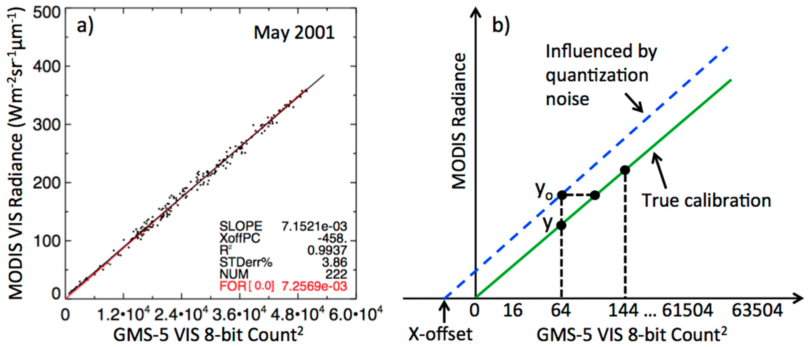
Figure 4.
Terra-to-Aqua-MODIS annual scaling factors (red circles). The Terra-MODIS radiance is multiplied by the scaling factor to predict the Aqua-MODIS radiance. The linear regression (black line) and associated statistics are also shown.
Figure 4.
Terra-to-Aqua-MODIS annual scaling factors (red circles). The Terra-MODIS radiance is multiplied by the scaling factor to predict the Aqua-MODIS radiance. The linear regression (black line) and associated statistics are also shown.

Figure 5.
(a) The Meteosat-9 clear-sky daily exoatmospheric radiance model (DERM) for Libya-4 observed during April 2007 and December 2012, where n is the number of daily observation. The statistics in the upper right corner display the percentage of the number of clear-sky observations. (b) The inter-annual variability of DERM during the 5.5-year window. The average daily inter-annual variability over all days of the year is 0.81%.

Figure 6.
(a) The monthly Met-9 deep convective cloud (DCC) visible count probability density functions (PDFs) of every 4th month starting in April 2007. The PDFs are color-coded by the indicated month. The number of monthly DCC pixels identified, the mean pixel-level count value, and the DCC-mode count value are also listed. (b) The monthly DCC-mean (red circles) and DCC-mode count (black circles) values are shown over the six-year Met-9 record.

Figure 7.
The first 5-year of monthly deep convective cloud (DCC)-mode Aqua-MODIS band 1 (0.65 µm) radiance results (Wm−2sr−1µm−1) organized by GEO domains. Tropical represents the entire tropical zone.
Figure 7.
The first 5-year of monthly deep convective cloud (DCC)-mode Aqua-MODIS band 1 (0.65 µm) radiance results (Wm−2sr−1µm−1) organized by GEO domains. Tropical represents the entire tropical zone.
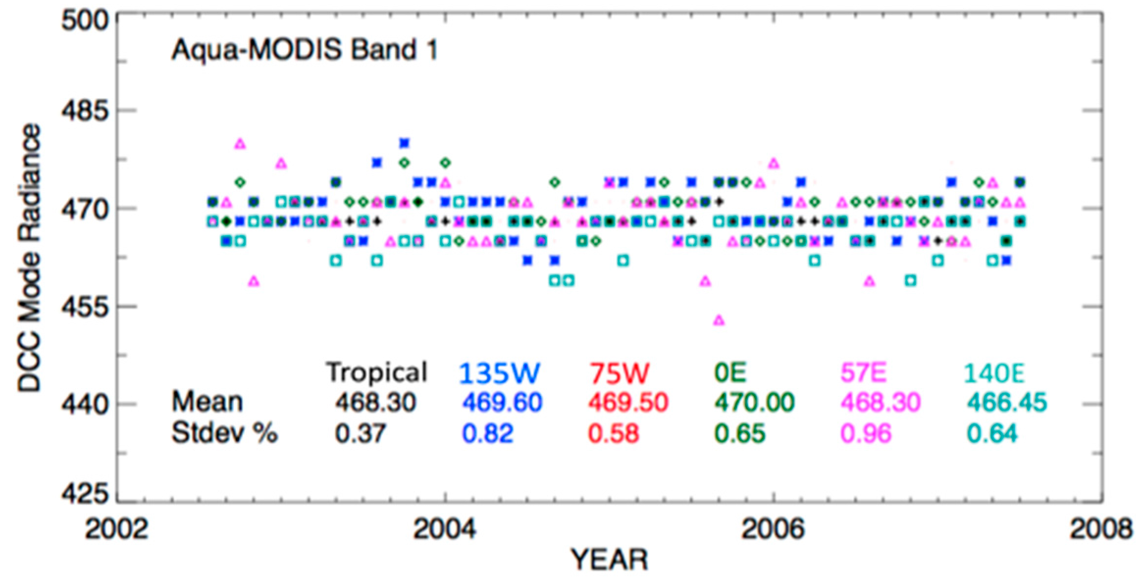
Figure 8.
The Aqua-MODIS band 1, Met-9 channel 1, and Met-7 visible channel spectral response functions.
Figure 8.
The Aqua-MODIS band 1, Met-9 channel 1, and Met-7 visible channel spectral response functions.

Figure 9.
The Met-9 channel 1 and Aqua-MODIS band 1 SCIAMACHY footprint pseudo radiance (Wm−2sr−1µm−1) pairs over: (a) all-sky tropical ocean (ATO); (b) clear-sky Libya-4; and (c) deep convective cloud (DCC). The StdErrReg% is the standard error about the fit and StdErrSlp% is the slope uncertainty. (d–f) The same as (a–c), respectively, except using Met-7 instead of Met-9.

Figure 10.
(a) Met-9; (b) Met-10; (c) GOES-12; (d) GOES-13; (e) GOES-8; and (f) Met-7 (57°E) all-sky tropical ocean ray-matching (ATO-RM), deep convective cloud (DCC)-RM, daily exoatmospheric radiance model (DERM), and DCC-mode monthly calibration gains and temporal trend lines. The temporal trend line coefficients (Equation (6)) are listed at the bottom of each plot, along with the DCC-RM, DERM, DCC-mode minus ATO-RM mean record gain differences (Diff%) and the monthly gain standard error (StdErr%) about the trend line.
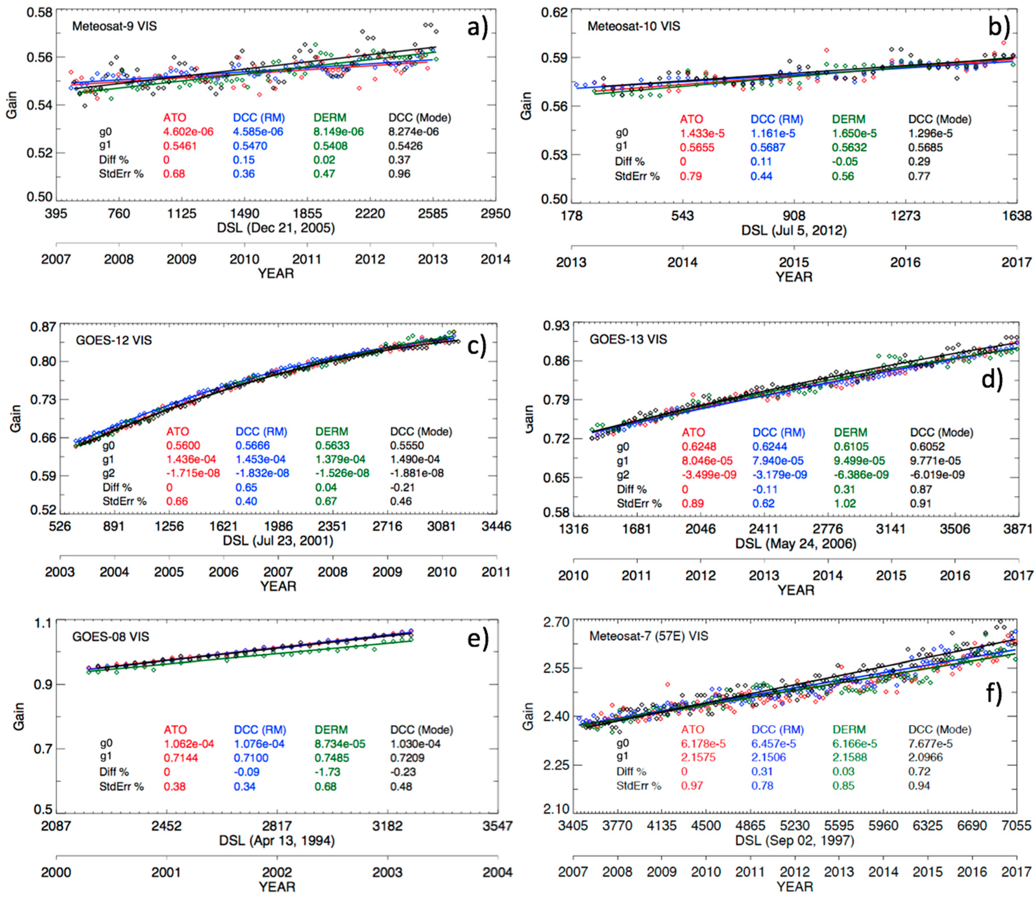
Figure 11.
(a) The daily exoatmospheric radiance model (DERM), deep convective cloud (DCC)-mode, and DCC-RM GEO record mean gain bias compared with all-sky tropical ocean ray-matching (ATO-RM); (b) the DERM, DCC-mode, DCC-RM minus ATO-RM monthly GEO gain RMS after removing the relative calibration bias; (c) the DERM, DCC-mode, DCC-RM, and ATO-RM GEO temporal trend standard errors; and (d) same as (a) with ±1 error bars. All y-axis units are in percent.

Figure 12.
The individual record mean deep convective cloud (DCC)-mode geostationary (GEO) radiance (Wm−2sr−1µm−1), plotted at the midpoint of the record, based on the all-sky tropical ocean ray-matching (ATO-RM) calibration and departure in percent from the five-year tropical mean DCC-mode MODIS radiance listed on the right of the plot. The uncertainty bars are from the GEO DCC-mode uncertainty.
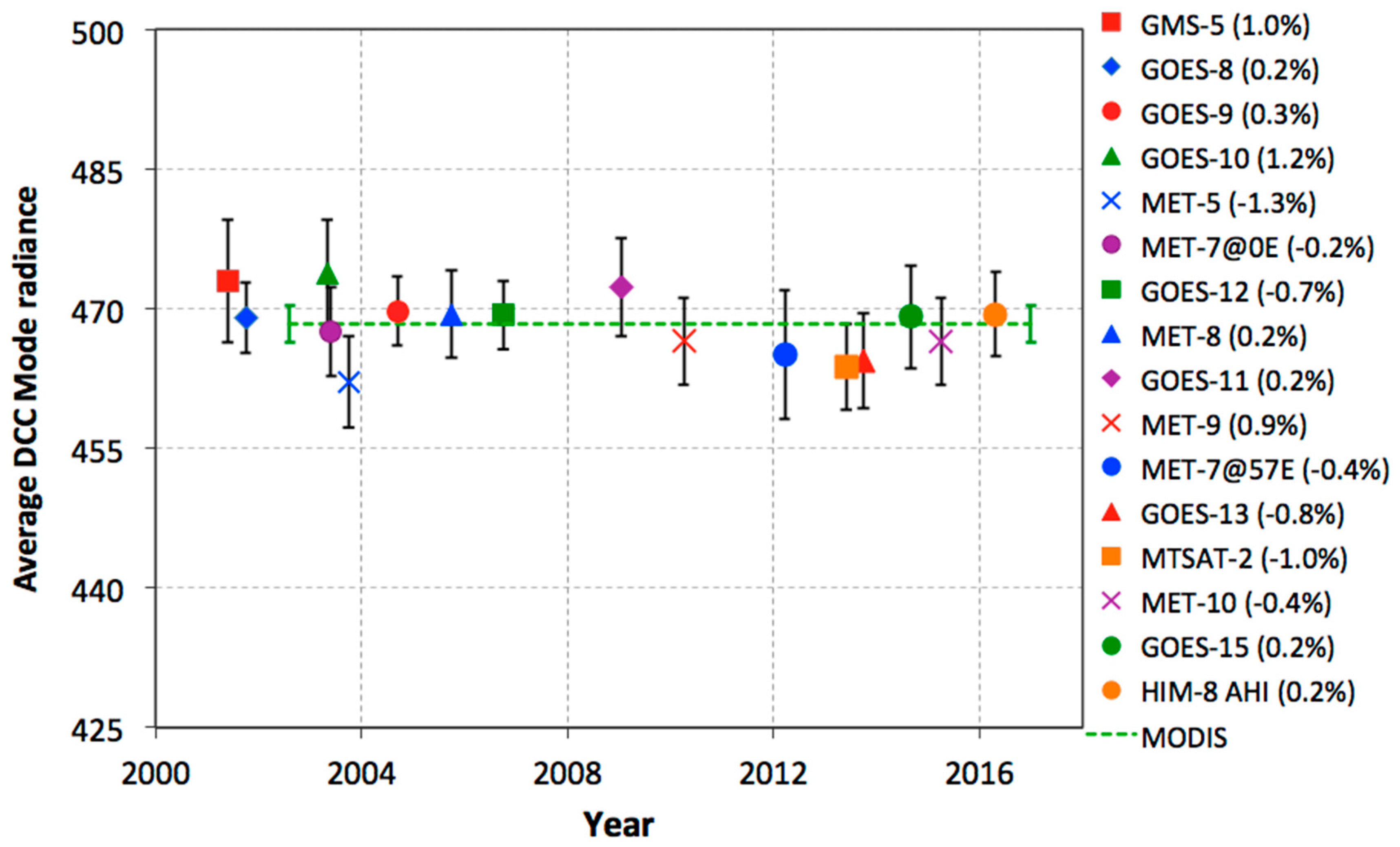

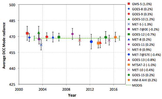
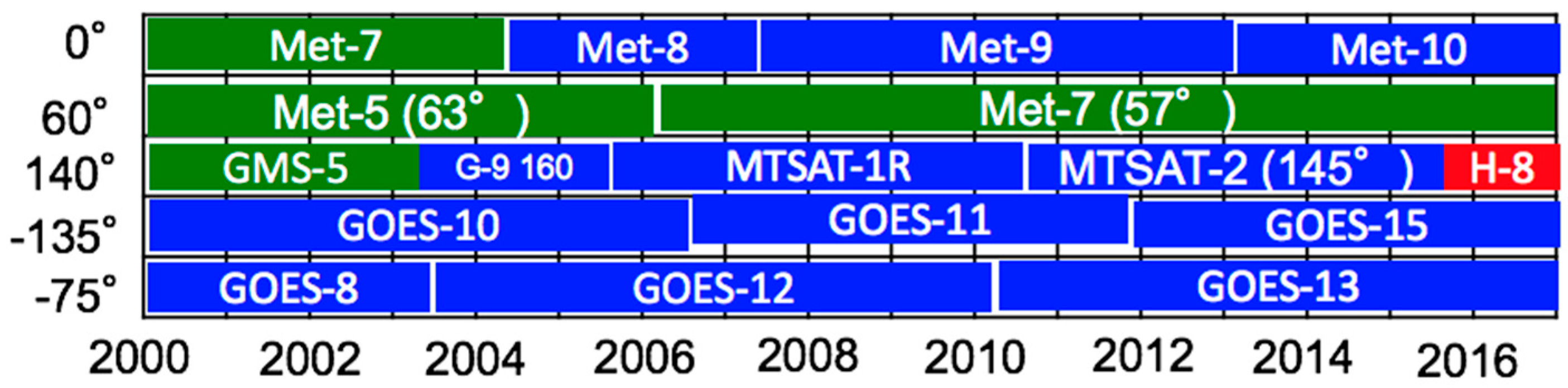
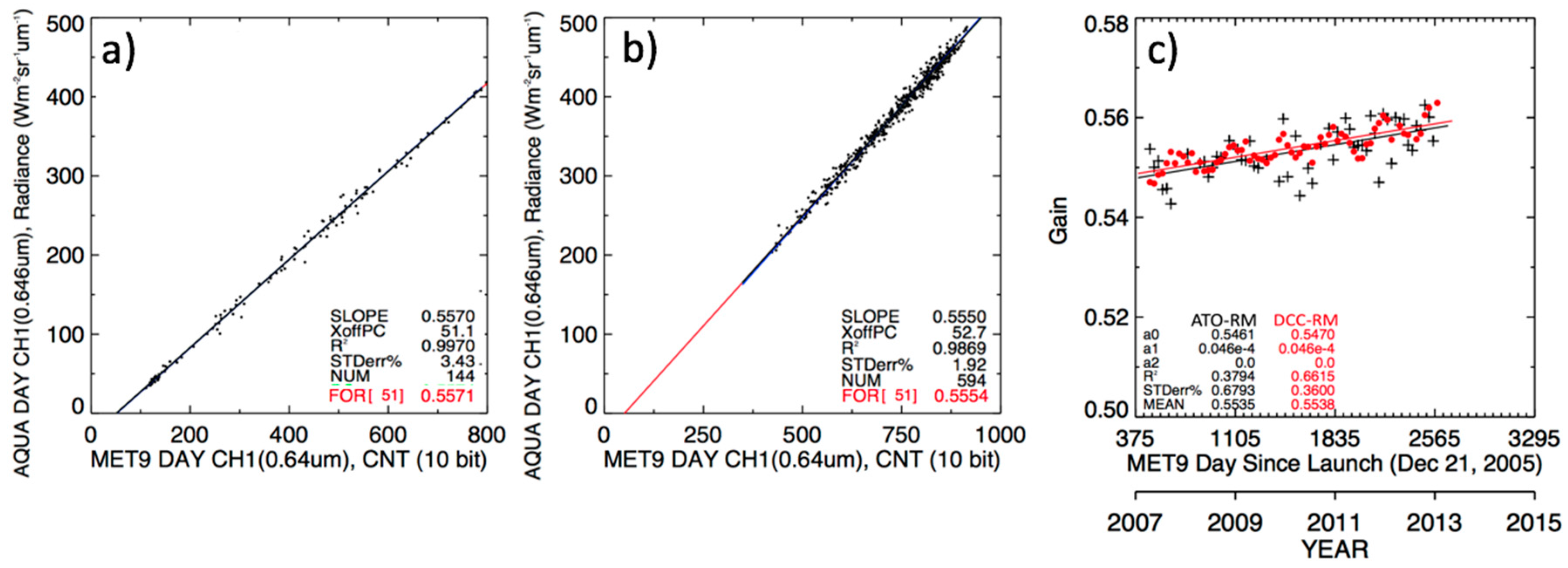
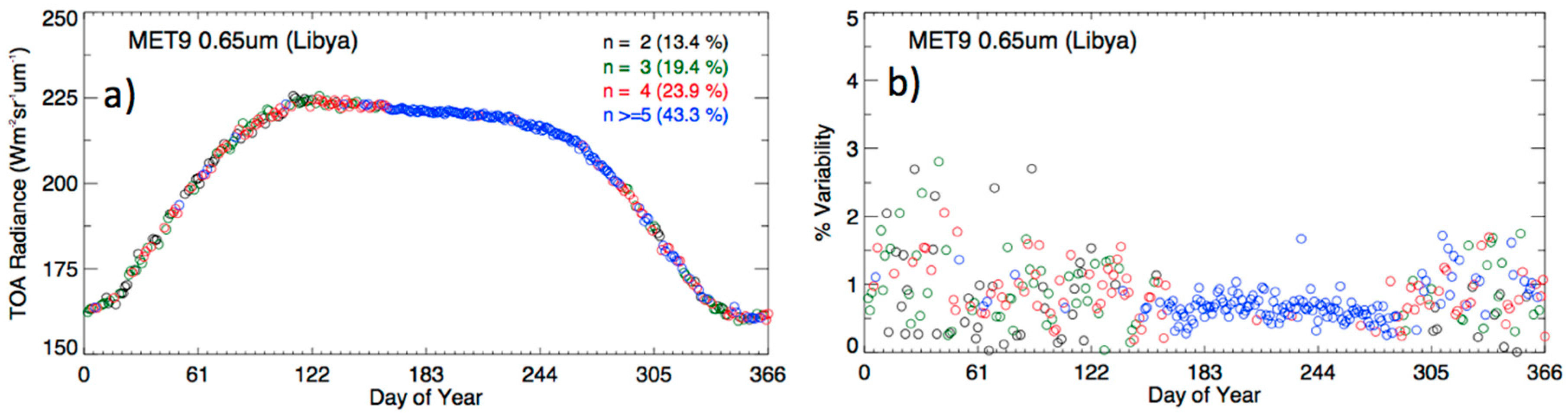
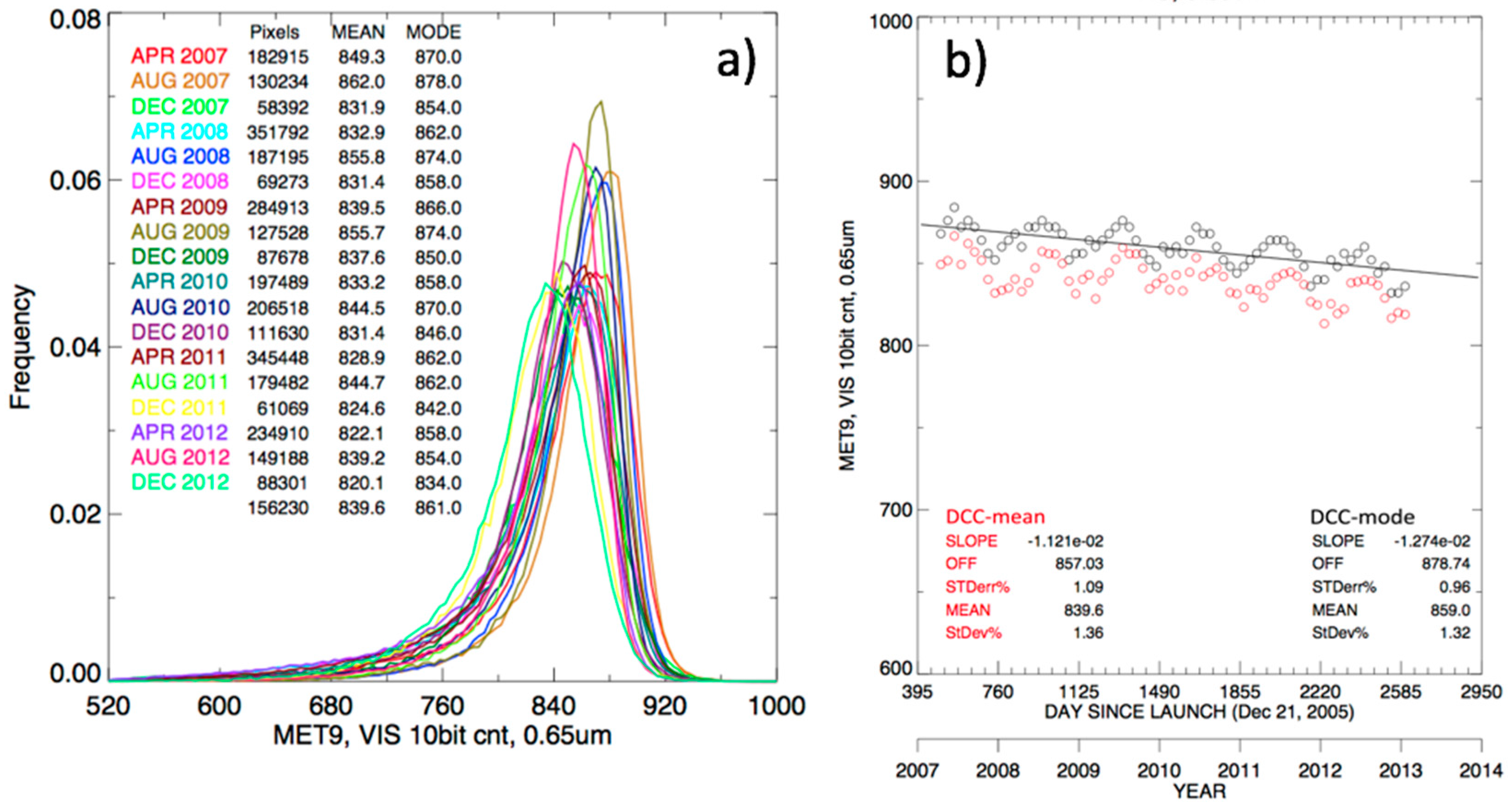
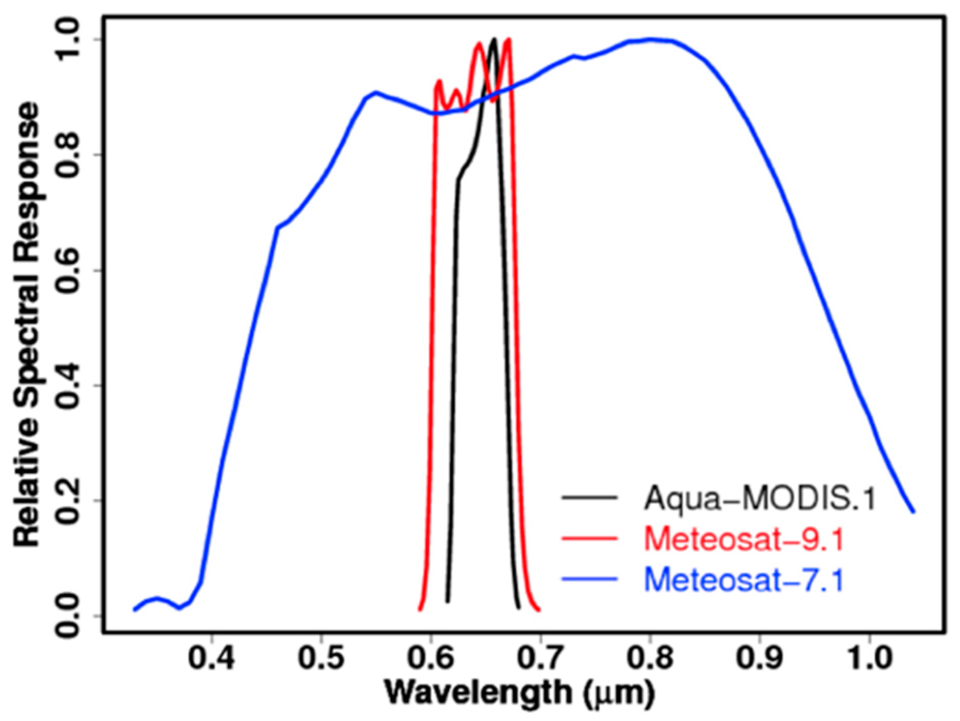
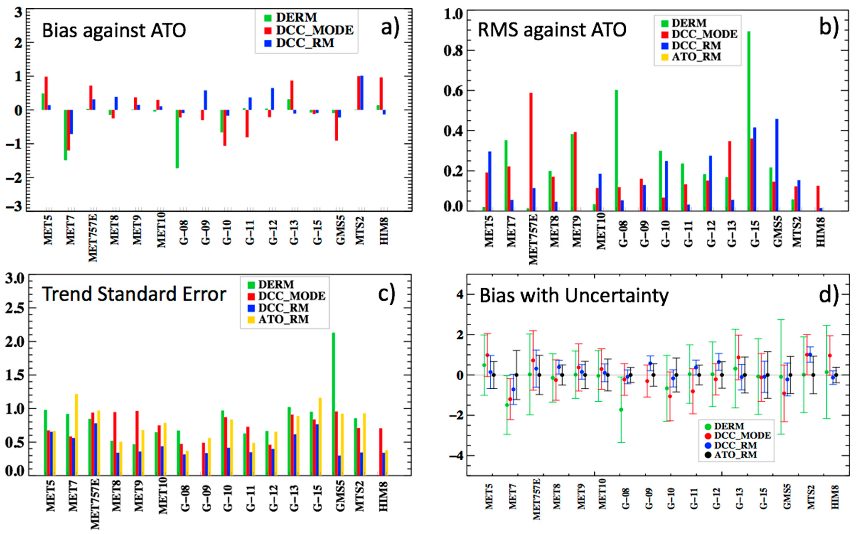
Table 1.
List of invariant desert targets by GEO domain. The center latitude and longitude are given, as well as the extent of the region of interest (ROI). The mean reflectivity and the standard deviation of the monthly reflectances (temporal stability) is based on GEODERM. The desert GEO viewing zenith angle (VZA), GEO image time in GMT (hh:mm), and the annual solar zenith angle (SZA) range observed at the given GMT are indicated. The DERM (σ) uncertainty is also listed.
| GEO Domain | 0°E | ~60°E | 140°E | 135°W | 75°W |
|---|---|---|---|---|---|
| GEODERM | Met-9 | Met-7 | MTSAT-2 | GOES-11 | GOES-12 |
| Desert | Libya-4 | Libya-4 | Badain | Sonoran | Sonoran |
| Center (Lat/Lon) | 28.6°/23.4°E | 28.6°/23.4°E | 40.1°/101.8°E | 32.0°/114.5°W | 32.0°/114.5°W |
| ROI | 0.5° × 0.5° | 0.5° × 0.5° | 0.4° × 0.4° | 0.2° × 0.2° | 0.2° × 0.2° |
| Reflectivity | 0.46 | 0.46 | 0.22 | 0.32 | 0.32 |
| Stability (%) | 1.0 | 1.0 | 1.6 | 1.0 | 1.0 |
| VZA | 42.1° | 49.5° | 60.8° | 43.4° | 56.4° |
| Reference Years | 2007–2012 | 2007–2015 | 2010–2015 | 2006–2011 | 2003–2010 |
| GMT | 10:30 | 10:30 | 05:30 | 19:30 | 19:30 |
| SZA range | 5–52° | 6–53° | 17–63° | 8–56° | 8–56° |
| DERM σ (%) | 0.81 | 1.50 | 1.40 | 1.21 | 1.30 |
Table 2.
The GEOsat equatorial longitude position, launch date, start and end year with month when the calibration coefficients in Table 3 are valid (whether the linear or squared count response is proportional to radiance), and the sensor response resolution in bits.
Table 2.
The GEOsat equatorial longitude position, launch date, start and end year with month when the calibration coefficients in Table 3 are valid (whether the linear or squared count response is proportional to radiance), and the sensor response resolution in bits.
| GEO | Longitude | Launch Date | Start Date | End Date | Count Response | Bit |
|---|---|---|---|---|---|---|
| GOES-8 | 75°W | 13 April 1994 | April 2000 | March 2003 | Linear | 10 |
| GOES-9 | 155°E | 23 May 1995 | May 2003 | October 2005 | Linear | 10 |
| GOES-10 | 135°W | 25 April 1997 | April 2000 | June 2006 | Linear | 10 |
| GOES-11 | 135°W | 3 May 2000 | August 2006 | November 2011 | Linear | 10 |
| GOES-12 | 75°W | 23 July 2001 | April 2003 | March 2010 | Linear | 10 |
| GOES-13 | 75°W | 24 May 2006 | April 2010 | December 2016 | Linear | 10 |
| GOES-14 1 | 75°W | 28 June 2009 | September 2012 | June 2013 | Linear | 10 |
| GOES-15 | 135°W | 4 March 2010 | December 2011 | March 2017 | Linear | 10 |
| MET-5 2 | 63°E | 2 March 1991 | May 2000 | January 2007 | Linear | 8 |
| MET-7 | 0E | 2 September 1997 | April 2000 | April 2006 | Linear | 8 |
| MET-7 3 | 57°E | 2 September 1997 | March 2007 | December 2016 | Linear | 8 |
| MET-8 | 3.4°E | 28 August 2002 | April 2004 | March 2007 | Linear | 10 |
| MET-9 | 0E | 21 December 2005 | April 2007 | December 2012 | Linear | 10 |
| MET-10 | 0E | 5 July 2012 | March 2013 | December 2016 | Linear | 10 |
| GMS-5 | 140°E | 17 March 1995 | May 2000 | May 2003 | Squared | 8 |
| MTSAT-1R 4 | 140°E | 26 February 2005 | July 2005 | October 2006 | Linear | 10 |
| MTSAT-1R 4 | 140°E | 26 February 2005 | November 2006 | December 2013 | Linear | 10 |
| MTSAT-2 | 145°E | 18 February 2006 | July 2010 | August 2015 | Linear | 10 |
| HIM-8 | 140.7°E | 7 October 2014 | July 2015 | December 2016 | Linear | 11 |
Table 3.
The CERES Ed4 GEO imager calibration coefficient offset (g0), linear (g1), and quadratic (g2) term, count offset (C0), visible band solar constant radiance (Esun) in Wm−2sr−1µm−1, and associated uncertainty (U) in percent.
Table 3.
The CERES Ed4 GEO imager calibration coefficient offset (g0), linear (g1), and quadratic (g2) term, count offset (C0), visible band solar constant radiance (Esun) in Wm−2sr−1µm−1, and associated uncertainty (U) in percent.
| GEO | Esun | g0 | g1 | g2 | C0 | U (%) |
|---|---|---|---|---|---|---|
| GOES-8 | 518.28 | 0.7144 | 1.062 × 10⁻⁴ | 0 | 29 | 0.4 |
| GOES-9 | 515.68 | 0.5209 | 8.286 × 10⁻⁵ | 0 | 29 | 0.6 |
| GOES-10 | 504.29 | 0.5106 | 1.898 × 10⁻⁴ | −2.334 × 10⁻⁸ | 29 | 0.8 |
| GOES-11 | 497.87 | 0.4945 | 6.804 × 10⁻⁵ | 0 | 29 | 0.5 |
| GOES-12 | 504.46 | 0.5600 | 1.436 × 10⁻⁴ | −1.715 × 10⁻⁸ | 29 | 0.7 |
| GOES-13 | 527.75 | 0.6248 | 8.046 × 10⁻⁵ | −3.499 × 10⁻⁹ | 29 | 0.9 |
| GOES-14 1 | 530.06 | 0.6378 | 4.420 × 10⁻⁵ | 0 | 29 | 0.7 |
| GOES-15 | 529.74 | 0.6803 | 8.673 × 10⁻⁵ | −3.041 × 10⁻⁹ | 29 | 1.2 |
| MET-5 2 | 446.07 | 1.6662 | 8.990 × 10⁻⁵ | −3.099 × 10⁻⁹ | 4.4 | 0.7 |
| MET-7 | 446.07 | 1.9156 | 2.123 × 10⁻⁴ | −2.195 × 10⁻⁸ | 4.95 | 1.2 |
| MET-7 3 | 446.07 | 2.1575 | 6.178 × 10⁻⁵ | 0 | 4.95 | 1.0 |
| MET-8 | 516.17 | 0.6208 | 9.560 × 10⁻⁶ | 0 | 51 | 0.5 |
| MET-9 | 516.07 | 0.5461 | 4.602 × 10⁻⁶ | 0 | 51 | 0.7 |
| MET-10 | 518.32 | 0.5655 | 1.434 × 10⁻⁵ | 0 | 51 | 0.8 |
| GMS-5 | 418.97 | 6.802 × 10⁻³ | 1.670 × 10⁻⁷ | 0 | 0 | 0.9 |
| MTSAT-1R 4 | 437.53 | 0.3881 | 5.293 × 10⁻⁴ | −6.471 × 10⁻⁷ | 0 | 2.1 |
| MTSAT-1R 4 | 437.53 | 0.4655 | 6.100 × 10⁻⁶ | 0 | 0 | 1.1 |
| MTSAT-2 | 479.33 | 0.4802 | 4.331 × 10⁻⁵ | 0 | 1 | 0.9 |
| HIM-8 | 517.21 | 0.2943 | 1.053 × 10⁻⁵ | 0 | 20 | 0.4 |
© 2018 by the authors. Licensee MDPI, Basel, Switzerland. This article is an open access article distributed under the terms and conditions of the Creative Commons Attribution (CC BY) license (http://creativecommons.org/licenses/by/4.0/).
Share and Cite
MDPI and ACS Style
Doelling, D.; Haney, C.; Bhatt, R.; Scarino, B.; Gopalan, A. Geostationary Visible Imager Calibration for the CERES SYN1deg Edition 4 Product. Remote Sens. 2018, 10, 288. https://doi.org/10.3390/rs10020288
AMA Style
Doelling D, Haney C, Bhatt R, Scarino B, Gopalan A. Geostationary Visible Imager Calibration for the CERES SYN1deg Edition 4 Product. Remote Sensing. 2018; 10(2):288. https://doi.org/10.3390/rs10020288
Chicago/Turabian StyleDoelling, David, Conor Haney, Rajendra Bhatt, Benjamin Scarino, and Arun Gopalan. 2018. "Geostationary Visible Imager Calibration for the CERES SYN1deg Edition 4 Product" Remote Sensing 10, no. 2: 288. https://doi.org/10.3390/rs10020288
Note that from the first issue of 2016, this journal uses article numbers instead of page numbers. See further details here.