A Deconvolution Technology of Microwave Radiometer Data Using Convolutional Neural Networks


1
School of Information and Electronic Engineering, Beijing Institute of Technology, Beijing 100081, China
2
National Satellite Meteorological Center, Beijing 100081, China
3
Faculty of Electrical Engineering, Delft University of Technology, 2628 CN Delft, The Netherlands
*
Author to whom correspondence should be addressed.
Remote Sens. 2018, 10(2), 275; https://doi.org/10.3390/rs10020275
Submission received: 1 December 2017
/
Revised: 23 January 2018
/
Accepted: 6 February 2018
/
Published: 10 February 2018
(This article belongs to the Section Remote Sensing Image Processing)
Abstract
:Microwave radiometer data is affected by many factors during the imaging process, including the antenna pattern, system noise, and the curvature of the Earth. Existing deconvolution methods such as Wiener filtering handle this degradation problem in the Fourier domain. However, under complex degradation conditions, the Wiener filtering results are not accurate. In this paper, a convolutional neural network (CNN) model is proposed to solve the degradation problem. The deconvolution procedure is defined as a regression problem in the spatial domain that can be solved with deep learning. For the real inverse process of microwave radiometer data, the CNN model has a more powerful reconstruction ability than Wiener filtering due to the multi-layer structure of the CNN, which enables the multiple feature transform of the data. Additionally, the complex degradation factor during the imaging process of a microwave radiometer can be solved with general framework-based learning. Experimental results demonstrated that the CNN model gains about 5 dB at the peak signal-to-noise ratio compared to the Wiener filtering deconvolution method, and can better distinguish the measured data.
1. Introduction
Compared to visible light and infrared remote sensing, the advantages of microwave remote sensing technology include the ability to capture images regardless of weather and light conditions [1], the ability to penetrate clouds and vegetation, being not easily affected by meteorological conditions or the level of sunshine, and the ability to detect ground targets. Microwave image data can provide information outside the infrared and the visible light image range. Therefore, it plays an important role in weather monitoring and disaster prediction. The microwave radiometer is one of the most important microwave remote sensing sensors. Due to the limitations on antenna size, system noise, and scanning mode, the image data obtained by microwave radiometers have low spatial resolution. However, low spatial resolution data does not satisfy the current needs; for example, the inversion of soil moisture [2] requires the low-frequency data of microwave imagers, while the spatial resolution of low-frequency data is low. Additionally, some geophysical parameters require the combination of brightness temperature data from different bands [3,4,5,6,7]. Therefore, improving the resolution of microwave radiometers using the deconvolution method is important.
The deconvolution of a microwave radiometer involves reconstructing an estimate of a brightness temperature image from the antenna temperature image. Two degradation factors are considered in the imaging process of microwave radiometers: the diffraction effect of the antenna pattern because the size is finite, and the overlap of footprints in the sampling process [8].
Many algorithms have been proposed for radiometer image deconvolution, such as the reconstruction technique in Banach spaces [9], the Backus–Gilbert (BG) inversion method [10], and scatterometer image reconstruction (SIR) [11]. These algorithms have been introduced to increase the spatial resolution of microwave radiometer image data. The reconstruction technique in Banach spaces enhances the spatial resolution by generalizing the gradient method. This approach allows the reduction of over-smoothing effects and oscillations without any reduction in the numerical complexity. The BG method uses redundant information from the footprint overlap region and prior knowledge of the antenna pattern to eliminate the overlap blur effect with an inverse matrix. The estimate of a brightness temperature image can be obtained from the antenna temperature image using a previously reported procedure [12,13,14,15]. The SIR algorithm is implemented through an iterative process to obtain the optimal estimate of brightness temperature as another form of multiplication algebra reconstruction technique (MART) [16,17]. Although these methods can achieve good performance, they are limited by the fact that the noise is also amplified when the resolution increases too much. Another deconvolution method using Wiener filtering was proposed to remove the diffraction blur due to the low-pass filtering effect of the antenna pattern. Wiener filtering can reconstruct the brightness temperature [18,19] using Fourier transform and filter theories to invert the convolution processing during the measurement procedure. However, serious ringing artifacts occur when the resolution increases past a certain point.
The image deconvolution of radiometer data is a challenging inverse problem, and the key is to obtain an optimal solution given the complex degradation conditions. Wiener filtering can eliminate the influence of the diffraction blur of the radiometer data using a deconvolution operation, but the noise is also amplified during this process [18]. Furthermore, due to the influence of the curvature of the Earth and many degradation factors, the deconvolution technology based on Wiener filtering needs further improvement [8]. Overall, Wiener filtering cannot achieve accurate reconstruction results.
In this paper, a deconvolution method based on the idea of deep learning is proposed to remove the diffraction blur caused by the antenna pattern. In addition, other degradation factors in the imaging process of the radiometer are solved using general framework-based learning. The deconvolution process is viewed as a nonlinear regression problem in a spatial domain different from the traditional Wiener filtering, which is designed by a filter model in the Fourier transform domain. The convolutional neural network (CNN)—a deep learning model—is used to directly learn deconvolution operations. In this procedure, the estimate of brightness temperature is obtained through feature extraction and multiple feature transform. Prior knowledge of the antenna pattern of the microwave radiometer is required for this process.
This work presents a significant step toward the practical use of microwave radiometer brightness temperature data. Existing algorithms have shown limited performance on measured data. The CNN deconvolution method obtains a more accurate estimate of brightness temperature images using a large number of data and prior knowledge, compared to the Wiener filtering method. It is essential that microwave radiometer data can be used effectively.
The outline of this paper is as follows. Section 2 describes the background of the proposed algorithm. The data used and related work are introduced in Section 3. The method for image deconvolution using CNN is described in Section 4. Experiments and results are described in Section 5 and Section 6, respectively, followed by a discussion and conclusions in Section 7 and Section 8, respectively.
2. Background
Deep learning [20] techniques are driving development in a variety of fields. For classical computer vision tasks such as image classification [21], image object detection [22], and image segmentation [23], deep learning methods have achieved very good results. Researchers have also proposed the use of deep learning techniques to improve the image quality of the natural environment. In Dong et al. [24], deep learning was proposed for image super-resolution using convolutional neural networks. This study presents the CNN model for directly learning end-to-end mapping between the low- and high-resolution images. The image super-resolution method based on CNN has been studied [25,26]. In Dietrich et al. [27], the convolutional neural network model was applied to image deburring. CNN have also achieved good results in image denoising [28,29].
Deep learning uses a multi-layer neural network to learn the internal features of an image and solves a variety of visual problems [30]. A universal remote sensing image quality improvement method using deep learning was reported [31]. In Ducournau and Fablet [32], the deep learning-based super-resolution algorithm was used to address ocean surface brightness temperature data. The research on deep learning techniques has demonstrated the potential of image restoration. However, little effort has been focused on remote sensing images, and especially microwave remote sensing images. In our work, for the radiometer image data degradation problem caused by the finite size of the antenna, the deep learning technique is proposed to improve the image quality of microwave radiometer brightness temperature data.
The microwave radiometer data are affected by many degradation factors, but existing deconvolution algorithms have some deficiencies. For example, the Backus–Gilbert (BG) algorithm is limited by noise amplification when reconstructing data. Wiener filtering needs different point spread functions (PSFs) to be designed to adapt to the change in the Earth’s curvature. These algorithms tend to solve one major degradation factor, whereas other factors require further processing. The degradation factors (e.g., the Earth’s curvature, system noise, and deformation caused by the antenna reflection surface) are relatively complicated during the actual working of the radiometer. Hence, in this case, the complexity of the deconvolution model increases and the reconstruction accuracy cannot be guaranteed.
For complex degradation during the imaging process, a CNN is expected to be able to accurately perform deconvolution operations on the radiometer data. During this process, the CNN simultaneously considers many kinds of degradation factors and then obtains accurate reconstruction results through multiple feature transformations. The contributions of this paper are as follows. (1) Aimed at the complex degradation of radiometer data, a deep learning-based general framework is proposed to address the degradation problem caused by a multitude of factors. (2) The CNN was found to be able to achieve higher reconstruction accuracy for radiometer data using multiple feature space transformation. (3) A flexible dataset creation method is proposed. By using the characteristics of the multiple radiometer frequency bands, the high-resolution channel data were selected as the ground truth image of the dataset to train the model.
3. Instrument and Related Work
The Fengyun-3 (FY-3) series is the second generation of Chinese polar orbiting meteorological satellites. The microwave radiation imager (MWRI) is an important spaceborne instrument on FY-3. The primary mission objectives of the MWRI include obtaining data about precipitation and cloud water, atmospheric precipitable water, sea surface temperature, soil moisture and temperature, and snow cover [33]. The data from MWRI were used for this study.
3.1. MWRI Instrument and Satellite Scan
The MWRI on-board the FY-3 satellite conically scans the Earth with a viewing angle of 45° and a swath of 1400 km. It is a high-sensitivity total power radiometer that obtains the brightness temperature data at five frequencies (10.65, 18.7, 23.8, 36.5, and 89.0 GHz), with each frequency having dual polarization [34]. The specific performance indicators of MWRI are shown in Table 1.
The MWRI ground resolution is related to frequency, and the high-frequency data have high ground resolution due to the beam width. The ground resolutions of the 10.65 GHz channel in a satellite orbit along and across the track direction are 85 and 51 km, respectively, and the ground resolution of the 89 GHz channel can be less than 20 km.
The scan geometry of the MWRI is shown in Figure 1. The satellite orbit height is 836 km, the ground incidence angle is 53°, and the observation angle is 45°. The MWRI antenna adopts a forward cone scanning method, so the entire observation field is elliptical rather than circular because of the incidence angle. In the observation field, the long axis △y is aligned with the direction of the satellite flight path, and the short axis △x is in the direction of the cross orbit. The Earth view sampling interval is 2.08 ms, and the integration times are 15, 10.0, 7.5, 5.0, and 2.5 ms from 10.65 to 89 GHz, respectively. Since the integration time is longer than the sampling time, some overlap exists between the antenna fields of view for all the channels, except for 89 GHz where both times are nearly equal [35].
In one scan, the MWRI can capture 254 observed brightness temperature data from the Earth [35]. An image file of 1600 × 254 pixels can be obtained with 1600 scans. However, the collected brightness temperature data are affected by the diffraction blur because of the low-pass filtering effect of the antenna pattern. An ideal approach is to use a larger antenna, but this is clearly not a reasonable and acceptable approach for satellite design. Therefore, an image deconvolution method is used to remove the diffraction blur and to optimally estimate the brightness temperature of the original scene. The overlap blur effects can also be suppressed in the process. This is a method that can be reasonably used to enhance spatial resolution.
3.2. Simulated Radiometric Measurement
The MWRI collects ground temperature information by receiving the electromagnetic waves radiated from the Earth’s surface. During the antenna scan, the true scene apparent temperature of the Earth’s surface is obtained. The antenna temperature can be represented by Equation (1):
where is the antenna temperature, is the apparent temperature, and represents the antenna pattern, is the effective aperture of the radio antenna, is the wavelength, and and denote the spherical coordinates on Earth.
Equation (1) can be converted into Equation (2) because the square of the wavelength to antenna effective aperture is the integral of the antenna pattern on .
As shown in Equation (2), the deconvolution reconstructs the apparent temperature from the antenna temperature .
A signal model for the radiometer is presented in Equation (3), which shows the degradation inherent in the imaging process. Due to the influence of the antenna pattern and the system noise, the antenna temperature can be considered as the convolution of the scene apparent temperature and the antenna pattern, plus the additive system noise n [36,37].
where is the apparent temperature, represents the antenna temperature, represents spatial coordinates, is the space-variant PSF instead of antenna pattern, is the convolution operator, and corresponds to radiometric noise NE△T. The antenna pattern uses a two-dimensional Gaussian function to make an ideal approximation. The radiometric noise is simulated by a random generation of noise values having Gaussian distribution, and the value of standard deviation is the NE△T corresponding to the frequency channel.
Equation (3) can be transformed into the Fourier domain by the discrete Fourier transform, so that the operation of convolution becomes a simple product in Equation (4).
4. Method
4.1. Radiometer Image Degradation
The impact of image degradation involves degradation factors that include the antenna pattern, system noise, and geometric deformation. As a priori information, these factors were included in the dataset through the image degradation process. In our study for feature learning, the 89 GHz antenna temperature image was used as the 18.7 GHz simulated apparent temperature. The 18.7 GHz simulated antenna temperature was obtained from the 18.7 GHz simulated apparent temperature and prior information based on Equation (3). The CNN directly estimates the apparent temperature image using the CNN model that was trained on the dataset. In the reconstruction process, the CNN considers a variety of degradation factors and is able to handle the connections among these factors. The PSF, which includes the geometric deformation and system noise in Equation (3), is described in detail below.
The 18.7 GHz channel antenna pattern was selected as the blur kernel, and the degradation image was obtained from the convolution between the 18.7 GHz simulated scene apparent temperature and the blur kernel. During deconvolution, the PSF was used to perform the convolution process, instead of directly using the antenna pattern function. The antenna pattern of the 18.7 GHz channel was determined by the half power beam width of the antenna, which is shown in Table 1. The PSF was simulated from the known 18.7 GHz antenna pattern by using a Gaussian function.
In the MWRI scanning process, the geometric parameters of the data in the same track direction are consistent, so in the PSF design, only the initial scan line was considered. To simulate the effects of the geometric deformation of the Earth on the data, 254 PSFs were used to degrade the entire image. This more closely aligns the degradation process to the actual imaging situation. The final reconstruction image consists of a line in each reconstruction image. The reconstruction mathematical expression is as follows:
where is a weighting function, is the estimate of apparent temperature, is the antenna temperature, and is the two-dimensional Fourier transform of the PSF. Q is the deconvolution function about . The weighting function—which chooses the right row in the image—is the Kronecker delta function. That is,
The PSF design contributes to image deconvolution and effectively enhances the edge. During Wiener filtering deconvolution [8], the calculation of each image requires many deconvolution operations that are time-consuming and highly complex. In our algorithm, the geometric deformation was seen as a priori information, and the PSF design was only executed in the degradation process of creating the dataset. The prior information was learned by the CNN model using a trained model, reducing the time requirement and complexity of the model.
The system noise was simulated by randomly generating Gaussian white noise. The value of the noise standard deviation of the specific channel is the NE△T, which is shown in Table 1. The NE△T of 18.7 GHz is 0.5 K, which was added to the image degradation process after the convolution operation.
The image degradation model was constructed with the PSF design, including the Earth’s geometric deformation and the system noise in the 18.7 GHz channel. The model can be implemented in the Fourier transform domain. The dataset was composed of the simulated scene apparent temperature and the degraded image obtained by the degradation model. Since the range of data of the MWRI is 0–340 K, it can be normalized to [0, 1] to achieve a faster convergence rate [38]. The normalized result was used to prepare the dataset for the deep neural network and model training.
where is the raw antenna temperature data, is the normalized data, is 0, and is 340.
In this section, a degradation model with multiple degradation factors is established. High-resolution 89 GHz channel data as the 18.7 GHz simulated apparent temperature was used to obtain the 18.7 GHz simulated antenna temperature by this degradation model. The 18.7 GHz simulated apparent temperature data and the 18.7 GHz simulated antenna temperature data constitute a dataset that contains a variety of prior information to train the model. In future work, this flexible method can build a real degradation model according to the actual situation.
4.2. Microwave Radiometer Image Deconvolution
The aim of radiometer image deconvolution is to obtain the optimal estimate of the original scene apparent temperature image from the antenna temperature image . As mentioned in the previous section, a diffraction blur occurs in the antenna temperature image due to the low-pass filtering effect of the antenna pattern. The deconvolution process is the inverse of the radiation measurement in Equation (3), where is obtained by assuming that , , and are known. As shown in Equation (8), the linear Wiener filtering is defined in the Fourier domain to obtain the optimal apparent temperature estimate:
In our algorithm, the microwave radiometer image deconvolution problem is defined as a regression problem in the spatial domain. From the Bayesian inference framework, the maximum a posteriori (MAP) finds the optimal scene apparent temperature .
where is the log-likelihood of antenna temperature , and corresponds to the prior distribution of . Equation (9) can be transformed to represent the loss function:
where can be obtained by minimizing the , and a regularization term can restrict the learning ability of model on the dataset so that the trained model has a stronger generalization ability for the new data. The larger the value of parameter , the greater the penalty for the model.
From the deep learning point of view, CNN is actually looking for a mapping relationship between to . The radiometric measurement information is included in the antenna temperature image. By knowing the detailed radiometric measurements, the hidden information can be found to estimate the apparent temperature image.
The proposed algorithm was implemented in two main steps. The first step was to establish the image degradation model by using the radiation measurement in Equation (3). For the known simulated apparent temperature, the observed antenna temperature image was obtained using the image degradation model. In the second step, the idea of deep learning was used to establish the CNN model to learn the mapping relationship between and , then the estimate of images were obtained. As the a priori information, the antenna pattern H and the system noise N are required for the image degradation model process. Compared to the design process of Wiener filter, the a priori information is not considered when establishing the CNN model process; it is only used in the first step to obtain .
4.3. Network Architecture
Convolutional neural networks (CNNs) are feed-forward artificial neural networks with strong feature extraction and mapping ability. For MWRI image deconvolution, the CNN model is adopted to learn mapping to obtain the estimate of the apparent temperature image. The network architecture of the proposed CNN is shown in Figure 2. In this CNN structure, three convolution layers are used: two layers for feature extraction and one for the reconstruction.
In each convolution layer, several convolution kernels are defined, which are used to carry the information from the real apparent temperature image to the antenna temperature image. In the convolution process, the input is a two-dimensional pixel matrix, and the convolution kernel moves over the entire image to produce the final output image, called the feature map. Each convolution layer has many convolution kernels, and each convolution kernel produces a corresponding feature map on the input image.
The rectified linear unit (ReLU) was chosen as an activation function for the first two convolution layers, since it has a faster convergence rate than the sigmoid activation unit [39]. Equation (11) is a ReLU function, where the output f can be obtained from x. Equation (12) is the activation function for the third convolution layer which is able to reconstruct the final output
Each convolutional layer plays a different role in the CNN model. Feature extraction and representation can be implemented in the first layer. This operation extracts overlapping patches from the antenna temperature image and represents each patch as a high-dimension vector. The second layer implements non-linear mapping. This operation nonlinearly maps each high-dimensional vector onto another high-dimensional vector. The final reconstruction process is completed in the last layer. This operation aggregates these high-resolution patch-wise representations to generate the final reconstructed temperature image. This image is expected to be similar to the ground truth apparent temperature.
During the training process, the input of the CNN model is the apparent temperature and the antenna temperature image, which can be degraded by the apparent temperature image. The main aim of training is to obtain the optimal weight parameters of the CNN model. For the trained CNN model, the antenna temperature image can be used as the input to obtain the apparent temperature image we expected. In this process, no preprocessing of the image is necessary.
5. Experiment
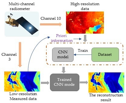
In this paper, the MWRI image deconvolution regression task was implemented by a supervised CNN model that could reconstruct the 18.7 GHz real scene apparent temperature from the observed antenna temperature images. The image deconvolution process is shown in Figure 3. Channels 1 to 10 correspond to the low-to-high-frequency bands in Table 1, respectively, so that channel 10 is 89 GHz with H polarization, and channel 4 is 18.7 GHz with H polarization.
The process contains three major steps: image degradation and dataset making, training and testing, and construction for the degraded image in the dataset and the real antenna temperature image. Image degradation is an important step, and simulates the generation of the observed images and contributes to the production of the dataset. The dataset is then used to train the CNN model. The trained CNN model reconstructs the degraded image in the dataset and in the 18.7 GHz measured image data.
In Section 3, the CNN framework was identified using a three-layer network architecture. In Long et al. [24], a typical set of parameters was determined. The first convolution layer had 64 convolution kernels, and the second convolution layer contained 32 convolution kernels. However, the observed MWRI targets were the Earth’s land, oceans, and other geographical objects. The edge changes of the temperature image are less complex than that of natural images. So, a set of alternative network parameters were used in our network structure. The number of convolution kernels in the first layer was 20, in the second layer was 10, and the experimental results showed that fewer convolution kernels still achieved good results, with a gain of about 5 dB at peak signal-to-noise ratio (PSNR) compared to the Wiener filtering deconvolution method.
To obtain better features, the antenna temperature image data of the 89 GHz channel—which contains 60 images from January to July 2017—was selected as the 18.7 GHz apparent temperature images dataset. The ground resolution of the selected image was 9 × 15 km, which is the highest resolution of all MWRI channels, meaning the temperature feature can be effectively extracted from these images. The dataset contained the degraded image, obtained by image degradation, in addition to the apparent temperature image. Ten images were randomly selected as the testing set, and the remaining 50 images served as the training set. In the training process, the images in the dataset were cropped to the size of the patch image (33,33). The input image size of the CNN model was (33,33), and the size of each convolution kernel was (9,9), so the output feature size was (33−9+1,33–9+1,20) in first layer, which is (25,25,20). The second layer had 10 kernels that were (5,5), so the size of output feature was (25–5+1,25–5+1,10), which is (21,21,10). In the final layer, a (5,5) convolution kernel was used to output the reconstruction image through the convolution operator, and the convolution kernel number of this layer was one. The size of the final output image was (17,17).
After the parameters were determined, backpropagation and stochastic gradient descendant (SGD) were used for training [40]. The training samples were divided into many minibatches to train the CNN model, and each minibatch had 128 training samples. In the training process of the experiment, the weight w could be updated with Equation (13) and (14):
where is the weight of next iteration after the ith iteration, v is the momentum variable, and is the gradient of the cost function with respect to the weights. In Equation (13), the base learning rate is 0.0001, the momentum is 0.9, and the weight decay is 0.0001. The weights were determined by the Gaussian distribution with standard deviation 0.001 in each layer.
The parameters of the CNN model were obtained following the training presented by Caffe [41], which is an open-source deep learning package. After the training procedure was finished, the optimal CNN model parameters were obtained. The estimate of the apparent temperature image was obtained from the input image using the trained CNN model. In the image degradation process, the PSF of the 18.7 GHz channel was selected as the degradation function for training, then the CNN model reconstructed the degraded images in the dataset as well as the real measured images of the 18.7 GHz channel. Figure 4 shows the internal reconstruction process used to estimate the apparent temperature image with the CNN model.
The reconstruction of this experiment contained two parts. The first part used the degraded images to reconstruct the corresponding estimate of apparent temperature images and evaluated the model. The second part input the 18.7 GHz real antenna temperature data into the trained CNN model to obtain the estimate of apparent temperature image.
The performance of the trained CNN model in the dataset is of key importance. The effect of the CNN model on the dataset must be monitored. However, the effect of reconstruction in the 18.7 GHz real measured data was also considered in our experiments, as it has more important engineering values for data usage. The goal of this work was for the trained model to ideally reconstruct both the measured data and the dataset.
6. Experimental Results
This part shows the experimental results that include the reconstruction results in the dataset and the real measured data in the 18.7 GHz channel. Before the results are displayed, the evaluation index of this work is outlined.
The image quality needs to be quantitatively described after the reconstruction of the dataset. Each pixel in the reconstruction image must be compared to that on the apparent temperature image, which served as a baseline image. The peak signal-to-noise ratio (PSNR) and structural similarity (SSIM) were chosen to evaluate the quality of the images and the effect of the trained model [42].
where and represent the temperature values of the baseline image and the awaiting evaluation image at the same location, respectively. Equation (15) shows the mean square error (MSE) which represents the difference between the reconstruction image and the high-resolution image. The PSNR calculation process is shown in Equation (16), which provides specific values to assess the quality of the reconstruction image. A larger value represents a better result.
SSIM measures the similarity of the structure between the two images, and the formula is shown in Equation (15). μ is the mean, is the standard deviation of I1, and is the covariance of I1 and I2. C is a constant used to ensure the stability of the formula. The SSIM value is between 0 and 1, and a value close to 1 represents a good image deconvolution effect.
The test images contained 10 scenes of images with 254 × 1000 pixels. The evaluation index is shown in Table 2, and the Wiener filtering deconvolution results are displayed as a comparison for the CNN model. As shown in Table 2, the PSNR results of the CNN model achieved an average increase of 5.63 dB compared to Wiener filtering. The average SSIM was also improved from 0.90 using Wiener filtering to 0.96 using the CNN model. Furthermore, the CNN model was faster than Wiener filtering, as the geometric deformation is simulated in the degradation process. Fewer calculations are required to obtain the results in the reconstruction procedure. The average run time was 1.23 s using the CNN model and 8.36 s using the Wiener filtering with an Intel i5 computer (the computer is from Lenovo Company in Beijing, China). The run time of CNN model is only related to the number of parameters in the CNN model. However, with Wiener filtering, the deconvolution operation requires multiple PSFs when the curvature of the Earth is considered, so the run time is influenced by the design of the PSF function. For example, for MWRI data, the deconvolution function contained 254 PSF when considering the curvature of the Earth.
Figure 5 shows the Caspian Sea area in test image 10. Figure 5b is the degraded image obtained from the convolution between Figure 5a and the 18.7 GHz antenna pattern. Details and edges of the area of Caspian Sea become unclear due to the effect of the antenna pattern. Figure 5c displays the result using the Wiener filtering method, showing that the contours of the Aral Sea became more apparent, but some details are missing. The CNN model reconstructed a better result than the Wiener filtering. The edges and contours of the lake and coastline were closer to the original image (Figure 5a) after the CNN reconstruction, suggesting that the diffraction blur caused by the antenna pattern can be further eliminated and more information can be obtained using this proposed method. Figure 6 and Figure 7 show the result for the local area in test images 9 and 7, respectively. The experimental results demonstrate that idea-based deep learning is effective at defining the MWRI image deconvolution problem as a regression problem in the spatial domain and solving this problem using the idea of deep learning.
In previous experiments, the CNN model was used and evaluated in the dataset. However, the validity of the CNN model for MWRI real measured data is still unknown. Figure 8 shows the experimental results for the MWRI 18.7 GHz real measured data in the Baltic Sea area. Figure 8b is the 36.5 GHz channel real measured data and the black square in the image contains Saaremaa Island and Hiiumaa Island. Their contour is visible due to the high ground resolution (18 × 30 km). However, the edge of these islands is not visible in Figure 8a due to the low ground resolution (30 × 50 km) of the 18.7 GHz channel. Figure 8c shows that the improvements due to Wiener filtering are very limited, though this method has long been proposed to solve the diffraction blur problem. Therefore, this result is insufficient for practical applications. A better result—as processed by the CNN model—is displayed in Figure 8d. The contour of Saaremaa Island is visible after the CNN model reconstruction. Although the reconstruction effect for Hiiumaa Island is less obvious, the reconstruction results of the CNN model were much better than the 18.7 GHz antenna temperature image (Figure 8a) and the reconstruction image (Figure 8c) with Wiener filtering.
In Figure 9, the 140th row of data from Figure 8 is displayed. The point near the 50th point of this row is the Saaremaa Island area. Due to low resolution, only one peak exists in this area of the 18.7 GHz data distribution curve, so distinguishing the two islands is impossible. This area is also indistinguishable using Wiener filtering in the distribution curve. However, the CNN reconstructed image has two peaks, like the 36.5 GHz image—a very effective improvement, as the CNN reconstructed image can distinguish the two islands. This also shows that the CNN reconstructed image is closer to the real ground scene and achieves a more significant effect on the real measured data than Wiener filtering.
7. Discussion
The ground truth data used in our experiments to train the CNN model was derived from the high-frequency band MWRI data. Because the 18.7 GHz ground apparent temperature is difficult to obtain for feature learning, the 89 GHz antenna temperature image was used as the 18.7 GHz simulated scene apparent temperature to learn the feature. This is a flexible approach that incorporates the multi-band radiometer data and provides a considerable amount of training data, which is also beneficial for CNN extraction features. Using this dataset, the CNN can be trained to obtain optimal model parameters. The experiment shows that the reconstruction results of this method were much better than Wiener filtering.
To obtain better training effects, we increased the number of images in the dataset, with a maximum of 150 images in the dataset. However, we found that too much data did not significantly improve the performance of the model. Using a dataset with 60 images, a good model was obtained. Continually increasing the number of images in the dataset only increased training time length. This result suggests that that the existing dataset covers enough temperature image features, and further increasing the number of images did not significantly contribute to the training of the model. In addition, since the 18.7 GHz ground truth apparent temperature was not available, we selected one row of data from the same position in Figure 8 in four plots to evaluate the performance of the proposed method. However, this is not an accurate evaluation method, which is a limitation of this experiment. This problem should be addressed in future work. In the design of the CNN model, the hyperparameter set of the CNN model is one of the most important factors to consider, including the number of kernels, size of kernels, and other training parameter settings. When experimentally tuning the model hyperparameters, different sizes of kernels were selected. We found that the size of kernels impacted the reconstructed image. For example, using a size nine kernel as the convolution kernel of the first layer achieved good results because a large kernel size can be more effective in extracting features, whereas increasing the kernel size also means increasing the number of parameters in the model. Therefore, the choice of network parameters is a trade-off between performance and speed.
8. Conclusions
In this paper, deep learning was proposed to implement deconvolution techniques for radiometer data. The CNN obtained a better deconvolution result and was more accurate for an end-to-end framework compared to Wiener filtering. For the training of the CNN model, the high-frequency high-resolution data was used as the ground truth image of the dataset, which includes degradation information in the low-frequency band. The proposed method can be adapted to a variety of degradation factors, so a more accurate degradation model that considers more degradation factors can be built into our approach. The deformation of the antenna during the operation of the satellite and the shake generated by the satellite platform affect the observed antenna temperature. These factors can be added to the degradation procedure in our algorithm in future work. This would improve the accuracy and generality of our deconvolution model. This model is also important for radiometer image engineering applications.
The image deconvolution method allows the subsequent use of radiometer data, including rainfall retrieval [43], sea ice concentration estimate [44], etc. From a satellite system engineering viewpoint, image deconvolution is a convenient and feasible method. It not only lifts the restrictions on satellite antenna size, but also improves the quality of low-resolution images in low bands. This paper proves the effectiveness of deep learning for radiometer image deconvolution, which shows potential for microwave remote sensing image processing.
Acknowledgments
This work is supported by Major Instrument Project of National Natural Science Foundation of China (Grants no. 61527805), Group Project of National Natural Science Foundation of China (Grants no. 61421001) and Project of Innovation & Introduced Intelligence for colleges and universities of China (Grants no. B14010). We are grateful to National Satellite Meteorological Centre for providing the data of MWRI and information of the instrument.
Author Contributions
Weidong Hu and Wenlong Zhang carried out the experiment and dataset making, and contributed to the research design and manuscript writing. Shi Chen performed data processing and manuscript writing. Xin Lv contributed to the simulation tools and co-supervised this study. Dawei An provided the FY-3 measured data. Leo P. Ligthart contributed to the research design and manuscript writing, and co-supervised this study.
Conflicts of Interest
The authors declare no conflict of interest.
References
- Ulaby, F.T.; Moore, R.K.; Fung, A.K. Volume 1-Microwave remote sensing fundamentals and radiometry. In Microwave Remote Sensing: Active and Passive; Artech House: Norwood, MA, USA, 1981; pp. 1223–1227. [Google Scholar]
- Bindlish, R.; Jackson, T.J.; Wood, E.; Gao, H.; Starks, P.; Bosch, D.; Lakshmi, V. Soil moisture estimates from trmm microwave imager observations over the southern united states. Remote Sens. Environ. 2003, 85, 507–515. [Google Scholar] [CrossRef]
- Wang, J.R.; Tedesco, M. Identification of atmospheric influences on the estimation of snow water equivalent from AMSR-E measurements. Remote Sens. Environ. 2007, 111, 398–408. [Google Scholar] [CrossRef]
- Grody, N.C. Classification of snow cover and precipitation using the special sensor microwave imager. J. Geophys. Res. Atmos. 1991, 96, 7423–7435. [Google Scholar] [CrossRef]
- Ferraro, R.R.; Smith, E.A.; Berg, W.; Huffman, G.J. A screening methodology for passive microwave precipitation retrieval algorithms. J. Atmos. Sci. 1996, 55, 1583–1600. [Google Scholar] [CrossRef]
- Pampaloni, P.; Paloscia, S. Microwave emission and plant water content: A comparison between field measurements and theory. IEEE Trans. Geosci. Remote Sens. 1986, 900–905. [Google Scholar] [CrossRef]
- Min, Q.; Lin, B. Remote sensing of evapotranspiration and carbon uptake at Harvard forest. Remote Sens. Environ. 2006, 100, 379–387. [Google Scholar] [CrossRef]
- Sethmann, R.; Burns, B.A.; Heygster, G.C. Spatial resolution improvement of SSM/I data with image restoration techniques. IEEE Trans. Geosci. Remote Sens. 1994, 32, 1144–1151. [Google Scholar] [CrossRef]
- Lenti, F.; Nunziata, F.; Estatico, C.; Migliaccio, M. On the spatial resolution enhancement of microwave radiometer data in banach spaces. IEEE Trans. Geosci. Remote Sens. 2014, 52, 1834–1842. [Google Scholar] [CrossRef]
- Backus, G.E.; Gilbert, J.F. Numerical applications of a formalism for geophysical inverse problems. Geophys. J. Int. 1967, 13, 247–276. [Google Scholar] [CrossRef]
- Long, D.G.; Hardin, P.J.; Whiting, P.T. Resolution enhancement of spaceborne scatterometer data. IEEE Trans. Geosci. Remote Sens. 1993, 31, 700–715. [Google Scholar] [CrossRef]
- Backus, G.; Gilbert, F. The resolving power of gross earth data. Geophys. J. Int. 1968, 16, 169–205. [Google Scholar] [CrossRef]
- Backus, G.; Gilbert, F. Uniqueness in the inversion of inaccurate gross earth data. Philos. Trans. R. Soc. Lond. 1970, 266, 123–192. [Google Scholar] [CrossRef]
- Farrar, M.R.; Smith, E.A. Spatial resolution enhancement of terrestrial features using deconvolved SSM/I microwave brightness temperatures. IEEE Trans. Geosci. Remote Sens. 1992, 30, 349–355. [Google Scholar] [CrossRef]
- Chakraborty, P.; Misra, A.; Misra, T.; Rana, S.S. Brightness temperature reconstruction using BGI. IEEE Trans. Geosci. Remote Sens. 2008, 46, 1768–1773. [Google Scholar] [CrossRef]
- Long, D.G.; Daum, D.L. Spatial resolution enhancement of SSM/I data. IEEE Trans. Geosci. Remote Sens. 1998, 36, 407–417. [Google Scholar] [CrossRef]
- Early, D.S.; Long, D.G. Image reconstruction and enhanced resolution imaging from irregular samples. IEEE Trans. Geosci. Remote Sens. 2001, 39, 291–302. [Google Scholar] [CrossRef]
- Sethmann, R.; Heygster, G.; Burns, B. Image Deconvolution Techniques for Reconstruction of SSM/I Data. In Proceedings of the International Geoscience and Remote Sensing Symposium, IGARSS, Remote Sensing: Global Monitoring for Earth Management, Espoo, Finland, 3–6 June 1991; pp. 2377–2380. [Google Scholar]
- Liu, D.; Liu, K. Resolution enhancement of passive microwave images from geostationary earth orbit via a projective sphere coordinate system. J. Appl. Remote Sens. 2014, 8, 98–109. [Google Scholar] [CrossRef]
- Lecun, Y.; Bengio, Y.; Hinton, G. Deep learning. Nature 2015, 521, 436. [Google Scholar] [CrossRef] [PubMed]
- Krizhevsky, A.; Sutskever, I.; Hinton, G.E. Imagenet classification with deep convolutional neural networks. In Proceedings of the International Conference on Neural Information Processing Systems, Lake Tahoe, NV, USA, 3–8 December 2012; pp. 1097–1105. [Google Scholar]
- Girshick, R. Fast R-CNN. arXiv, 2015; arXiv:arXiv:1504.08083. [Google Scholar]
- Long, J.; Shelhamer, E.; Darrell, T. Fully convolutional networks for semantic segmentation. In Proceedings of the 2015 IEEE Conference on Computer Vision and Pattern Recognition (CVPR), Boston, MA, USA, 7–12 June 2015; pp. 3431–3440. [Google Scholar]
- Dong, C.; Chen, C.L.; He, K.; Tang, X. Learning a Deep Convolutional Network for Image Super-Resolution; Springer International Publishing: Berlin, Germany, 2014; pp. 184–199. [Google Scholar]
- Kim, J.; Lee, J.K.; Lee, K.M. Deeply-recursive convolutional network for image super-resolution. In Proceedings of the 2016 IEEE Conference on Computer Vision and Pattern Recognition (CVPR), Las Vegas, NV, USA, 27–30 June 2016; pp. 1637–1645. [Google Scholar]
- Shi, W.; Caballero, J.; Huszár, F.; Totz, J.; Aitken, A.P.; Bishop, R.; Rueckert, D.; Wang, Z. Real-time single image and video super-resolution using an efficient sub-pixel convolutional neural network. In Proceedings of the 2016 IEEE Conference on Computer Vision and Pattern Recognition (CVPR), Las Vegas, NV, USA, 27–30 June 2016; pp. 1874–1883. [Google Scholar]
- Schuler, C.J.; Burger, H.C.; Harmeling, S.; Schölkopf, B. A machine learning approach for non-blind image deconvolution. In Proceedings of the 2013 IEEE Conference on Computer Vision and Pattern Recognition, Portland, OR, USA, 23–28 June 2013; pp. 1067–1074. [Google Scholar]
- Burger, H.C.; Schuler, C.J.; Harmeling, S. Image denoising: Can plain neural networks compete with BM3D? In Proceedings of the 2012 IEEE Conference on Computer Vision and Pattern Recognition, Providence, RI, USA, 16–21 June 2012; pp. 2392–2399. [Google Scholar]
- Zhang, K.; Zuo, W.; Gu, S.; Zhang, L. Learning deep CNN denoiser prior for image restoration. In Proceedings of the 2017 IEEE Conference on Computer Vision and Pattern Recognition (CVPR), Honolulu, HI, USA, 21–26 July 2017; pp. 2808–2817. [Google Scholar]
- Bengio, Y. Learning deep architectures for AI. Found. Trends Mach. Learn. 2009, 2. [Google Scholar] [CrossRef]
- Wei, Y.; Yuan, Q.; Shen, H.; Zhang, L. A universal remote sensing image quality improvement method with deep learning. In Proceedings of the 2016 IEEE International Geoscience and Remote Sensing Symposium (IGARSS), Beijing, China, 10–15 July 2016; pp. 6950–6953. [Google Scholar]
- Ducournau, A.; Fablet, R. Deep learning for ocean remote sensing: An application of convolutional neural networks for super-resolution on satellite-derived sst data. In Proceedings of the 2016 9th IAPR Workshop on Pattern Recogniton in Remote Sensing (PRRS), Cancun, Mexico, 4 December 2016; pp. 1–6. [Google Scholar]
- Yang, Z.; Lu, N.; Shi, J.; Zhang, P.; Dong, C.; Yang, J. Overview of FY-3 payload and ground application system. IEEE Trans. Geosci. Remote Sens. 2013, 50, 4846–4853. [Google Scholar] [CrossRef]
- Wu, S.; Chen, J. Instrument Performance and Cross Calibration of FY-3C MWRI. In Proceedings of the 2016 IEEE International Geoscience and Remote Sensing Symposium (IGARSS), Beijing, China, 10–15 July 2016; pp. 388–391. [Google Scholar]
- Yang, H.; Weng, F.; Lv, L.; Lu, N.; Liu, G.; Bai, M.; Qian, Q.; He, J.; Xu, H. The fengyun-3 microwave radiation imager on-orbit verification. IEEE Trans. Geosci. Remote Sens. 2011, 49, 4552–4560. [Google Scholar] [CrossRef]
- Paola, F.D.; Dietrich, S. Resolution enhancement for microwave-based atmospheric sounding from geostationary orbits. Radio Sci. 2008, 43. [Google Scholar] [CrossRef]
- Dietrich, S.; Paola, F.D.; Bizzarri, B. MTG: Resolution enhancement for MW measurements from geostationary orbits. Adv. Geosci. 2006, 7, 293–299. [Google Scholar] [CrossRef]
- Goodfellow, I.; Bengio, Y.; Courville, A. Deep Learning; MIT Press: Cambridge, MA, USA, 2016. [Google Scholar]
- Nair, V.; Hinton, G.E. Rectified Linear Units Improve Restricted Boltzmann Machines. In Proceedings of the International Conference on International Conference on Machine Learning, Bangalore, India, 9–11 February 2010; pp. 807–814. [Google Scholar]
- Melorose, J.; Perroy, R.; Careas, S. Efficient backprop. Neural Netw. Tricks Trade 2015, 1524, 9–50. [Google Scholar]
- Jia, Y.; Shelhamer, E.; Donahue, J.; Karayev, S.; Long, J.; Girshick, R.; Guadarrama, S.; Darrell, T. Caffe: Convolutional architecture for fast feature embedding. In Proceedings of the ACM International Conference on Multimedia, Glasgow, Scotland, 1–4 April 2014; pp. 675–678. [Google Scholar]
- Wang, R.; Tao, D. Recent progress in image deblurring. arXiv, 2014; arXiv:arXiv:1409.683. [Google Scholar]
- Farrar, M.R.; Smith, E.A.; Xiang, X. The impact of spatial resolution enhancement of SSM/I microwave brightness temperatures on rainfall retrieval algorithms. J. Appl. Meteorol. 1994, 33, 313–333. [Google Scholar] [CrossRef]
- Zhang, S.; Zhao, J.; Frey, K.; Su, J. Dual-polarized ratio algorithm for retrieving arctic sea ice concentration from passive microwave brightness temperature. J. Oceanogr. 2013, 69, 215–227. [Google Scholar] [CrossRef]
Figure 1.
The scan geometry of the MWRI.

Figure 2.
The architecture of the proposed convolutional neural network (CNN).

Figure 3.
Microwave radiation imager (MWRI) image deconvolution algorithm flow chart.

Figure 4.
The reconstruction internal process of the estimate of apparent temperature image by the CNN model.
Figure 4.
The reconstruction internal process of the estimate of apparent temperature image by the CNN model.

Figure 5.
Experimental results for the Caspian Sea area in test image 10 of the dataset: (a) The 18.7 GHz simulated scene apparent temperature image; (b) The 18.7 GHz simulated antenna temperature image; (c) Wiener reconstructed image from the 18.7 GHz simulated antenna temperature image; and (d) the CNN reconstructed image from the 18.7 GHz simulated antenna temperature image.

Figure 6.
Experimental results for test image 9 of the dataset: (a) the 18.7 GHz simulated apparent temperature image; (b) the 18.7 GHz simulated antenna temperature image; (c) Wiener reconstructed image from the 18.7 GHz simulated antenna temperature image; and (d) CNN reconstructed image from the 18.7 GHz simulated antenna temperature image.

Figure 7.
Experiment results for test image 7 of the dataset: (a) the 18.7 GHz simulated apparent temperature image; (b) the 18.7 GHz simulated antenna temperature image; (c) the Wiener reconstructed image from the 18.7 GHz simulated antenna temperature image; and (d) the CNN reconstructed image from the 18.7 GHz simulated antenna temperature image.

Figure 8.
Experimental results for the Baltic Sea area with 18.7 GHz real measured data: (a) the 18.7 GHz antenna temperature image; (b) the 36.5 GHz antenna temperature image: (c) Wiener reconstructed image from the 18.7 GHz antenna temperature image; and (d) the CNN reconstructed image from the 18.7 GHz antenna temperature image.

Figure 9.
The distribution curve of real measured data of 18.7 GHz.


Table 1.
Performance of the microwave radiation imager (MWRI).
| Center Frequencies (GHz) | Polarization | Ground Resolution (km) | Beam Width | NE△T (K) |
|---|---|---|---|---|
| 10.65 | V/H | 51 × 85 | 2.03/2.01 | 0.5 |
| 18.7 | V/H | 30 × 50 | 1.17/1.18 | 0.5 |
| 23.8 | V/H | 27 × 45 | 1.17/1.18 | 0.5 |
| 36.5 | V/H | 18 × 30 | 0.62/0.62 | 0.5 |
| 89 | V/H | 9 × 15 | 0.29/0.29 | 1 |
Table 2.
The evaluation index of the test images in the dataset. PSNR: peak signal-to-noise ratio; SSIM: structural similarity.
Table 2.
The evaluation index of the test images in the dataset. PSNR: peak signal-to-noise ratio; SSIM: structural similarity.
| Evaluation Index | Test Image | Wiener | CNN | Test Image | Wiener | CNN |
|---|---|---|---|---|---|---|
| PSNR/dB | Image 1 | 33.50 | 38.72 | Image 6 | 35.77 | 40.83 |
| SSIM | 0.8827 | 0.9549 | 0.9153 | 0.9667 | ||
| Time/s | 8.44 | 1.21 | 8.29 | 1.24 | ||
| PSNR/dB | Image 2 | 33.29 | 38.89 | Image 7 | 34.99 | 40.9 |
| SSIM | 0.8789 | 0.9567 | 0.9238 | 0.9718 | ||
| Time/s | 8.33 | 1.29 | 8.24 | 1.21 | ||
| PSNR/dB | Image 3 | 34.96 | 40.28 | Image 8 | 33.97 | 39.51 |
| SSIM | 0.9078 | 0.9636 | 0.8989 | 0.9596 | ||
| Time/s | 8.58 | 1.23 | 8.3 | 1.21 | ||
| PSNR/dB | Image 4 | 35.84 | 40.79 | Image 9 | 35.49 | 40.6 |
| SSIM | 0.9113 | 0.9658 | 0.9037 | 0.9642 | ||
| Time/s | 8.32 | 1.26 | 8.66 | 1.28 | ||
| PSNR/dB | Image 5 | 31.42 | 39.67 | Image 10 | 34.91 | 40.25 |
| SSIM | 0.9223 | 0.9692 | 0.9064 | 0.9638 | ||
| Time/s | 8.17 | 1.23 | 8.28 | 1.2 | ||
| PSNR/dB | Average | 34.41 | 40.04 | |||
| SSIM | 0.9051 | 0.9636 | ||||
| Time/s | 8.36 | 1.23 |
© 2018 by the authors. Licensee MDPI, Basel, Switzerland. This article is an open access article distributed under the terms and conditions of the Creative Commons Attribution (CC BY) license (http://creativecommons.org/licenses/by/4.0/).
Share and Cite
MDPI and ACS Style
Hu, W.; Zhang, W.; Chen, S.; Lv, X.; An, D.; Ligthart, L. A Deconvolution Technology of Microwave Radiometer Data Using Convolutional Neural Networks. Remote Sens. 2018, 10, 275. https://doi.org/10.3390/rs10020275
AMA Style
Hu W, Zhang W, Chen S, Lv X, An D, Ligthart L. A Deconvolution Technology of Microwave Radiometer Data Using Convolutional Neural Networks. Remote Sensing. 2018; 10(2):275. https://doi.org/10.3390/rs10020275
Chicago/Turabian StyleHu, Weidong, Wenlong Zhang, Shi Chen, Xin Lv, Dawei An, and Leo Ligthart. 2018. "A Deconvolution Technology of Microwave Radiometer Data Using Convolutional Neural Networks" Remote Sensing 10, no. 2: 275. https://doi.org/10.3390/rs10020275
Note that from the first issue of 2016, this journal uses article numbers instead of page numbers. See further details here.