Radiometric Correction of Close-Range Spectral Image Blocks Captured Using an Unmanned Aerial Vehicle with a Radiometric Block Adjustment


Finnish Geospatial Research Institute, National Land Survey of Finland, Geodeetinrinne 2, 02430 Masala, Finland
*
Author to whom correspondence should be addressed.
Remote Sens. 2018, 10(2), 256; https://doi.org/10.3390/rs10020256
Submission received: 25 November 2017
/
Revised: 16 January 2018
/
Accepted: 3 February 2018
/
Published: 7 February 2018
(This article belongs to the Special Issue Recent Progress and Developments in Imaging Spectroscopy)
Abstract
:Unmanned airborne vehicles (UAV) equipped with novel, miniaturized, 2D frame format hyper- and multispectral cameras make it possible to conduct remote sensing measurements cost-efficiently, with greater accuracy and detail. In the mapping process, the area of interest is covered by multiple, overlapping, small-format 2D images, which provide redundant information about the object. Radiometric correction of spectral image data is important for eliminating any external disturbance from the captured data. Corrections should include sensor, atmosphere and view/illumination geometry (bidirectional reflectance distribution function—BRDF) related disturbances. An additional complication is that UAV remote sensing campaigns are often carried out under difficult conditions, with varying illumination conditions and cloudiness. We have developed a global optimization approach for the radiometric correction of UAV image blocks, a radiometric block adjustment. The objective of this study was to implement and assess a combined adjustment approach, including comprehensive consideration of weighting of various observations. An empirical study was carried out using imagery captured using a hyperspectral 2D frame format camera of winter wheat crops. The dataset included four separate flights captured during a 2.5 h time period under sunny weather conditions. As outputs, we calculated orthophoto mosaics using the most nadir images and sampled multiple-view hyperspectral spectra for vegetation sample points utilizing multiple images in the dataset. The method provided an automated tool for radiometric correction, compensating for efficiently radiometric disturbances in the images. The global homogeneity factor improved from 12–16% to 4–6% with the corrections, and a reduction in disturbances could be observed in the spectra of the object points sampled from multiple overlapping images. Residuals in the grey and white reflectance panels were less than 5% of the reflectance for most of the spectral bands.
Keywords:
UAV; UAS; drone; hyperspectral; calibration; photogrammetry; radiometry; BRDF; radiometric correction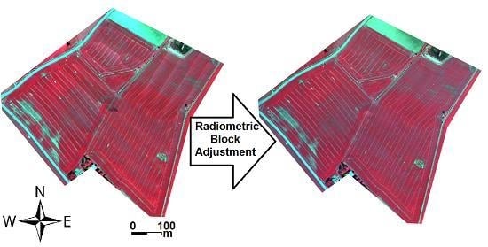
1. Introduction
Unmanned Aerial Vehicles (UAVs, drones) equipped with miniaturized multi- and hyperspectral imaging sensors offer completely new possibilities for carrying out close-range remote sensing tasks [1]. Using these technologies, spectral remote sensing measurements can be made cost-efficiently, with greater accuracy and detail than ever before. Several pushbroom hyperspectral imaging sensors [2,3,4,5,6] and point spectrometers [7,8] have recently been implemented in UAVs. Hyperspectral cameras based on the 2D frame format sensors have entered the market in recent years, offering an interesting alternative for hyperspectral data capture [9,10,11,12,13,14,15]. Commercially available sensors and products include for example the Rikola Hyperspectral Camera [16] and the Cubert UHD 185-Firefly [17]. Multi-spectral cameras based on 2D format sensors are also being rapidly developed, such as the Parrot Sequoia [18].
This study focuses on the radiometric calibration and correction of close-range 2D frame format image datasets captured using drones. The approach in a drone remote sensing campaign is to capture an image block with overlapping image strips and overlapping images within each strip while flying over the area of interest, providing multiple overlapping views of each object point. The complete image over the object is obtained by orthorectifying the images and combining them to a mosaic [19]. Using the 2D format images, 3D point clouds or the object 3D geometric model can also be created [20] together with spectral data [13]. The images typically do not provide a uniform radiometric response as a result of many disturbances in the imaging process [12,21,22,23,24,25]. In order to utilize the radiometric information of hyper- and multispectral data in quantitative analysis, such as in the analysis of object condition or a comparison of multi-temporal and multi-sensorial data acquisitions, the data has to be radiometrically calibrated so that information from all individual images are at the same scale and comparable.
Measuring reflectance in passive imaging is a complex process, one influenced by lighting conditions, scattering processes in the atmosphere and the surrounding environment, adjacent objects, and finally, the spectral, directional (typically anisotropic) reflectance characteristics of the object itself and the topography of the object [23,24,25] (Figure 1). Under practical conditions, in airborne and space-borne remote sensing applications, the direct reflected solar radiance (Lsu), reflected diffuse (sky) radiance (Lsd) and the atmospheric path radiance (Lsp) are generally considered as the major components of the at-sensor radiance entering the sensor (Ls_at_sensor), and they form the basis of the conventional rigorous correction methods [23,24,25]. In the close-range imaging from UAVs and terrestrial vehicles, the atmospheric path radiance (Lsp) has minor impact because of the short path length. In the shadowed areas, Lsu is non-existent and other radiance components dominate. Further components of Ls_at_sensor include the reflected background radiance (Lsbg), the multiple radiance reflected first by the background objects and then by the atmosphere (Lsbg_mult) and the radiance from adjacent objects. Comprehensive studies about impacts and significance of these factors under different conditions in the case of UAV based close-range spectrometry are still missing, and this is important topic for future studies.
Corrections for the atmospheric and illumination conditions are required in order to transform image grey values (DN) to reflectance. In the classical physically based correction approach, a radiometrically-calibrated sensor is the prerequisite [23,24,25]. The fundamental calibration parameters include the photon response nonuniformity correction (PRNU) to compensate for the vignetting effects and the nonuniformity of the detector [4,13,14,15,23,24]; the sensor calibration parameters may also include the absolute calibration model from DNs to physical units of radiance. For absolutely calibrated sensors, the physically based atmospheric correction can be utilized; corrections for the path radiance, impacts of the adjacent objects and irradiance levels can be estimated utilizing the atmospheric radiative transfer codes, such as Modtran or 6S and the insitu observations of weather conditions [25,26,27]. Important challenges in the use of this approach in typical UAV operating scenarios include the missing calibration and potential instability of the UAV sensors and the fact that UAVs are often operated at low altitudes, where cloudy weather conditions are typical. Therefore, the empirical line method [28] is highly relevant for UAV applications, because it replaces the need for modeling the atmospheric effects and the illumination level via a simple linear transformation; furthermore, absolute radiance calibration of the sensor is not required. As most natural objects display anisotropic reflectance characteristics [29], further corrections are needed to compensate for these effects by utilizing a bidirectional reflectance distribution function (BRDF) based correction. In steep environments, the topographic effects must also be corrected [14,23,24,25]. In the final step, shadow correction is performed if necessary [30].
In recent studies, the radiometric correction of UAV imagery and spectrometry has mostly emphasized the atmospheric correction using reflectance panels [6,12,13,14,15,31,32,33,34,35,36,37], atmospheric radiative transfer modeling [2,4] or normalization of UAV based radiance observations using field based radiance observations of a reference panel or irradiance [7,8,31]. Aasen et al. [13] and Yang et al. [15] calibrated the Cubert UHD 185-Firefly hyperspectral imagery; they emphasized the sensor calibration and performed reflectance calibration using single or multiple reflectance panels. To cope with varying illumination conditions, methods based on continuous illumination monitoring are highly relevant; in previous studies either ground based [7,31] or onboard-based solutions [8,31] have been used. These studies have reported about challenges related to the irradiance sensor calibration and tilting during the flights. Disturbances due to the object reflectance anisotropy have been corrected from 2D frame format images using statistical approaches, such as dodging [37,38], or using the model based BRDF correction [12,32,33,34,35,36]. Jakob et al. [14] presented a processing toolbox for 2D frame format images suitable for a mine exploration environment; the radiometric corrections included the sensor corrections as well as the topographic correction that accounted for the influences of terrain topography; the reflectance transformation was carried out using the empirical line method.
The previous studies have offered only partial solutions for the radiometric correction process, by mostly considering the sensor calibration and the atmospheric correction. We have developed a radiometric block adjustment-based approach to carry out radiometric correction and to provide homogeneous reflectance data from 2D frame format hyperspectral drone image datasets [12,32]. The approach is to model the radiometric imaging process and its disturbances and then solve the parameters of this model using least squares optimization utilizing the redundant observations; all fundamental factors can be included in the single, combined adjustment task. The outputs of the process are the radiometric model parameters, which are used to produce radiometrically corrected image products, such as reflectance mosaics, reflectance point clouds or multi-view and -angular reflectance observations of objects of interest. Similar approaches have previously been used with aircraft images [39,40,41,42]. We have used the radiometric block adjustment method already in various applications, including for agricultural and forest use [12,32,33,34,35,36]. In those studies, the weather included different combinations of sunny, cloudy or variable conditions. The objective of this investigation is to implement and investigate an extended, combined radiometric block adjustment method, and specifically, to study in detail the weighting (or stochastic model) aspects when correcting UAV image blocks captured in an agricultural environment. The method and an empirical study conducted using a dataset captured over a winter wheat canopy are described in Section 2. The results of the study are presented in Section 3 and discussed in Section 4. The results show that the method performed consistently and clearly improved the homogeneity of the image blocks.
2. Materials and Methods
2.1. Radiometric Block Adjustment of UAV Image Blocks
The radiometric block adjustment method used in this study was previously developed by Honkavaara et al. [12,32]. In this study we extended the model to allow different solar elevations (Equations (4), (6) and (10)) and we integrated the reflectance panel observations (Equation (8)) to the combined model. In order to be able to combine various observations optimally in the calculation process, it was necessary to develop the comprehensive stochastic model, i.e., weighting of different observations (Equations (12)–(16)). In the following, we present the extended combined model and the weighting scheme, and the practical implementation of the method.
2.1.1. Radiometric Model
The following formulation assumes that the sensor radiometric disturbances have been corrected based on sensor calibration information. The current approach utilizes empirical line method for the reflectance transformation. This approach was selected because there are many uncertainties in physically-based reflectance retrieval, and the reflectance targets provide a simple approach for reflectance transformation. The complete model for the image DN accounting for the variability of the radiance measurement and the BRDF effects is given for image j and object k as follows:
where is the reflectance factor for specific view/illumination geometry, is the incident illumination zenith angle; is the reflection view zenith angle; is the relative azimuth angle, where and are the azimuth angles of reflected and incident light, respectively; and are the linear parameters to transform reflectance to DN; and are the relative image-wise gain and offset parameters; in this study we are using only the parameters. The definition for the reflectance factor is the hemispherical directional reflectance factor (HDRF) [22].
can be presented using the vertical reflectance of the object at the specific solar illumination angle, , and the anisotropy factor, . The anisotropy factor is derived as the ratio of the modelled directional and vertical reflectance, and , respectively [43]:
where is a selected sun illumination angle that appeared during the campaign. In our current implementation, we use the simple empirical BRDF model developed by Walthall et al. [44] and Nilson and Kusk [45]. Previously, the model was used by Beisl et al. [43,46] with 1D pushbroom and 2D frame format images. The 3-parameter model, , is feasible for data collected during a short period of time (Equation (3)), but an extended version, , is used for cases with a varying sun zenith angle (Equation (4)):
where , m = 1, …, 4, are the BRDF parameters. A hot-spot term can also be included [45], but such an option is not used in this particular study. In the adjustment, the anisotropy factor is used, which reduces the number of BRDF parameters for the 3-parameter model to 2. The anisotropy factors for models 3 and 4, respectively, are given as follows:
The complete error equation for a radiometric tie point is as follows:
In addition to the radiometric tie points, other observations can also be included to the combined adjustment. In the current implementation, we use radiometric control points (RCP) (reflectance panels) to calculate the reflectance transformation. The error equation for RCP k with reflectance and reflectance observation is as follows:
In order to avoid instability of the calculation, the relative parameters and the BRDF parameters (in the 4-parameter case; Equation (4)) are also treated as weighted observations. The error equation for the relative image-wise gain parameter with an observation is given as follows:
Error equations for the BRDF parameters are formed for each m (m = 1, …, 4) parameter with observation :
An optimal solution can be calculated using nonlinear weighted regression by minimizing the weighted sum of residuals [47]:
where is the vector of unknowns, is the weight matrix i.e., the stochastic model (Section 2.1.2), is the design (Jacobian) matrix, including the derivatives of the functional model with respect to unknowns, and is the vector of observations.
The unknowns of the model can be summarized as follows:
- Absolute reflectance transformation parameters for the entire block: ,
- image-wise relative correction parameters for number-of-images—1 images (one of the images is selected as the reference image): , ;
- BRDF model parameters: , m = 1, …, number-of-parameters;
- nadir reflectance for each radiometric tie point k: .
Relevant parameters are selected for each adjustment task. For example, during overcast conditions it is not necessary to use the BRDF model, whereas under stable conditions the relative correction parameters are not usually necessary.
2.1.2. Weighting the Observations
The weighting of the observations, has considerable impact on the fitting process [47]. The rule of employing weights is to adjust the impact of using observations with different relative accuracies. For independent observations, the corresponding weights are considered based on a priori known standard deviations. By employing this scheme, an observation with a larger standard deviation will less contribute in the adjustment result. For independent observations, the weights are introduced to the fitting process as the diagonal elements in the matrix W. One of the objectives of this investigation is to study impacts of different weighting settings. The practical values used for the dataset in this study are presented in Section 2.4.2.
The weight of an image observation of a radiometric tie point () is based on the standard deviation of the image observation () scaled by the image DN:
where is the a priori standard deviation of unit weight. is defined separately for each object type and spectral band based on expected variations in the tie point windows. Based on our experience, feasible values are 0.05–0.10 for crops and 0.2–0.3 for forest; furthermore, variations are larger in the sunny conditions than in overcast conditions due to the impacts of shadows, specular reflection and other impacts.
The weight for the relative image-wise correction parameter () is based on the estimated variation of the illumination conditions and the estimated quality of the a priori estimates ():
The weights for the RCPs () are based on the estimated standard deviation of the reference reflectance observations ():
The weights for the BRDF parameters (; m = 1, …, 4) are based on the estimated standard deviations of the a priori values of parameters ():
The a priori standard deviation of the unit weight is calculated for the desired object type as follows:
where is considered as the expected reflectance for selected object type, for example, the average reflectance spectra of canopy under study. This setting impacts only to the a posteriori stochastic model of the adjustment. When considering weight of an image DN (Equation (12)), it can be seen that if the DN represents average object reflectance in the area, the corresponding radiometric tie point has the unit weight (1.0).
2.1.3. Implementation
In a typical radiometric block adjustment task for mosaic generation, a uniform grid of radiometric tie points is generated in the ground coordinate system utilizing the digital surface model (DSM) from the area so that 20–100 tie points appear in each image. In order to take DNs from the images, the image coordinates of the tie points are calculated in each image using the collinearity equation augmented with the radial and tangential lens distortion parameters [19]. The visibility of the radiometric tie point in each image is checked. For flat environments, such as agricultural fields, a simple projection of the XYZ coordinates in images is sufficient; for complex environments, such as forest, the analysis of the 3D environment is often needed. If a point is visible in a certain image, then the observation equation is formed; an average DN within an image window of suitable size is used as the radiometric tie point observation. The image observations of the RCPs are obtained similarly; the reflectance reference is based on a laboratory or in situ measurement of the targets with a spectrometer. Observations for the relative parameters can be based on drone or terrestrial irradiance measurements [31], or else a constant value (e.g., 1.0) can be used. The least squares method is then run to find the optimal values for the unknowns. Each spectral band is processed separately. After solving the radiometric model parameters, the radiometric output products are calculated, such as hyperspectral orthophoto mosaics or hyperspectral point clouds.
Inputs to the processing include the images corrected using the laboratory based radiometric corrections, the image geometric model parameters (camera interior orientations and lens distortions and exterior orientations of images), the 3D model of the object (a DSM or point cloud), the coordinates of the reflectance panels and the reflectance spectra, information of the solar angles and the irradiance information for each image if available. The user gives parameters of the processing, including the radiometric model, radiometric tie point window size, distribution of the radiometric tie points, as well as the a priori standard deviations of observations for the weighting purposes. All this information is given in input files and afterwards the entire processing is carried out automatically. After adjustment, the statistical analysis of the results can be carried out using statistical tools of the least squares regression. The results are evaluated using different statistics, such as the values and the a posteriori standard deviations of the parameters, and uniformity statistics.
The radiometric block adjustment has been developed as C++ software at the Finnish Geospatial Research Institute (FGI). It is part of the complete UAV image data processing environment, including image pre-processing tools, photogrammetric software for geometric processing and GIS software for data analysis.
2.2. Agricultural Test Site
Dataset for the empirical study was captured in an agricultural test site in southern Finland, in the city of Vihti (355466 E, 6701384 N; the ETRS-TM35FIN coordinate system); the site belongs to the Natural Resources Institute Finland. The area of interest was approximately 20 ha and was covered with winter wheat; the canopies were in a pre-heading stage thus the top layers were mainly formed by leaves (Figure 2a).
For geo-referencing purposes, a total of 15 GCPs were targeted using circular targets with a 30 cm diameter. They were measured using the virtual reference station real-time kinematic GPS (VRS-GPS) method with accuracies (RMSE) of approximately 3 cm in the X and Y coordinates and 4 cm in the Z coordinates [48]. Black, grey and white reflectance reference panels of a size of 1 m × 1 m and a nominal reflectance of 0.03, 0.09 and 0.50 [49] were deployed in the area. The targets were organized into two groups for all targets (W1,G1,B1; W2,G2,B2) and four white targets were distributed to different parts of the area (Wf1; Wf2; Wf3; Wf4) (Figure 2b). Altogether 21 vegetation samples were used when evaluating the spectral quality; their measured dry biomass range was 0.9 to 266.5 g·m−2, with an average and median of 126.4 g·m−2 and 122.0 g·m−2, respectively.
2.3. UAV Campaign
An octocopter UAV with a MikroKopter autopilot was used (Figure 2a). Its payload capacity was 1.5 kg, and the maximum flight time was 10 min. A tunable Fabry-Pérot Interferometer (FPI) based hyperspectral camera was used for the image capture (the model 2012b owned by the FGI) [9,10,11,12]. The camera weighs about 700 g and has an image size of 1024 × 648 pixels, an 11 μm pixel size and a focal length of 10.9 mm; the image field of view (FOV) is ±18° in the flight direction, ±27° in the cross-flight direction and ±31° at the format corner. GPS and irradiance sensors were fixed to the frame of the UAV and connected to the imager. The spectral range of the imager is 500–900 nm, and the spectral channels can be selected flexibly for each application. In this study, 35 bands were captured with a full width at half maximum (FWHM) of 24–32 nm (Table 1).
The UAV flight campaign was carried out on 23 May 2014. The area was covered with four flights during a time period of 2.5 h (Table 2). The flying altitude was 100 m above ground level, giving a ground sampling distance (GSD) of 10 cm. The number of images capture during each flight was 100–200. The forward overlaps were 68–74% and the side overlaps were 51–60%. The resulting view-zenith angles in the output mosaics were mostly less than ±15° but in some areas the view zenith angles were up to ±25° (Figure 3a); it is expected that these large view angles will cause anisotropy effects in the mosaics. The largest view zenith angles appeared between the flight lines; within the flight lines the view zenith angles were mostly less than ±5°.
An irradiance sensor based on the Intersil ISL29004 photodetector with a spectral sensitivity range of 400–1000 nm was integrated into the camera to measure the irradiance during each exposure. Since the sensor is not calibrated, relative, broadband irradiance intensity values can be obtained [31]. Consistent with our previous experience, the flight direction influenced the irradiance recording due to the tilting of the irradiance sensor with respect to the sun’s illumination, because the tilt compensation was not applied. This caused large variability in the irradiance recordings (Figure 3b). Some low irradiance values appeared during flights f3 and f4 (indicated with arrows in Figure 3b), which were due to the clouds blocking the sun’s illumination. Only a few images were captured in cloud shadow during the experiments, which could be eliminated from the analysis process. In the following analysis flights f3 and f4 are combined because they were captured within 20 min time period; the combined dataset is referred as f34. Medians of the irradiance observations were used as a priori irradiance levels of the flights in the processing (shown as dashed lines in Figure 3b). The a priori value for the parameter was calculated for each flight as the ratio of the median of the irradiances of each flight j () and the selected reference flight ()
2.4. Data Processing Chain
The entire processing chain for the FPI imagery has been developed in previous studies [12,32,33,34,35] and it includes the following steps:
- Applying radiometric laboratory calibration corrections to images;
- Determining the orientation parameters of the images;
- Using dense image matching to create a DSM;
- Determining a radiometric imaging model;
- Calculating the hyperspectral image mosaics.
In the following sections, the geometric (2–3) and radiometric (1, 4, 5) processing steps used in this investigation are described.
2.4.1. Geometric Processing
During the geometric processing phase, the orientations of selected three reference bands (bands 2, 13 and 24 in Table 1) were first determined using the Agisoft PhotoScan Professional commercial software (AgiSoft LLC, St. Petersburg, Russia). All flights were processed separately. The outputs of the process included the camera calibrations (Interior Orientation Parameters—IOP, including the models for the lens distortions), the exterior orientations of each image (Exterior Orientation Parameters—EOP) and the 3D object coordinates of the tie points; they were transformed to the ETRS-TM35FIN coordinate system using the GCPs for the area. The dense DSM was calculated using the PhotoScan software with a better than 10 cm point interval. Reprojection errors as a result of the PhotoScan processing were approximately 0.5 pixels or less, which indicated good accuracy (Table 3). Point densities in the dense point clouds were 107–157 points/m2. EOPs of the remaining 32 unaligned bands were calculated automatically by matching to the reference bands using the in-house software; this procedure provided subpixel accuracy in the band alignment [50].
2.4.2. Radiometric Processing
The sensor corrections included the correction for vignetting and other sensor nonuniformities, which were determined in the laboratory and the dark current correction that was determined using a black image taken before each flight [9].
The radiometric block adjustment method was used to calculate the radiometric imaging model. Different parametrizations were used (the case numbers refer to Table 4):
- Absolute calibration via the empirical line method for each of flights: f1, f2 and f34 (el3) and the combined flight f34 (el1); cases 1, 5;
- el3 or el1 and BRDF correction; cases 2, 6;
- or el1 and BRDF and relative image-wise corrections (); cases 3, 7;
- full model with absolute calibration and BRDF and corrections; cases 4, 8.
The above cases 2–4 included the radiometric block adjustment. In the cases 1–3, the empirical line parameters were calculated using panels measured in a single image. In the case 4, the absolute calibration parameters were treated as unknowns and solved in the adjustment; the panels were measured in all images where the view zenith angle to the panel was smaller than 10°. The calculations were performed for the full dataset (flights f1, f2, f34) and for the dataset consisting of flight f34. In the former dataset, the full four-parameter BRDF model (Equation (4)) was used, whereas for the latter dataset only the three parameter model was used (Equation (3)).
A uniform grid of tie points was generated in the area with a 15 m point interval; this provided approximately 25 radiometric tie points for each image. In most cases, the DN observation of the radiometric tie point was calculated using an image area of 30 × 30 pixels (3 m × 3 m at object), but tie point areas of 10 × 10 pixels (1 m × 1 m) and 2 × 2 pixels (0.20 m × 0.20 m) were also evaluated. The image observations for RCPs were calculated as the average for an object area with a size of 0.20 m × 0.20 m.
The impacts of the observation weighting and other settings were studied empirically using green (L0 = 549.6 nm), red (L0 = 663.8 nm) and NIR (L0 = 794.0 nm) bands. The tested settings are based on considerations of feasible values and experience gained in our earlier studies and the present dataset (Table 5). The values were 0.05, 0.10 and 0.20, indicating expected precision of approximately 5%, 10% and 20% of the a priori parameter values. For , values of 0.05 and 0.10 were used, indicating a 5% and 10% variation within the window, which is feasible for homogeneous crop canopies. Two different a priori values were used for the BRDF parameters. The major analyses were made using (m = 1, …, 4) of 20, 50 or 100% of the a priori values, and also another weighting approach was used; BRDF observations were included to the adjustment for the first time and they were investigated in this study. The values were 0.01 and 0.001 in reflectance units. To calculate (Equation (16)), the expected reflectance was set to 0.05 in the red and green wavelengths and 0.30 in the NIR range. The a priori values for the were calculated based on the medians of the irradiance recordings by the Intersil radiometer during the flights (Equation (17)) or a constant value of 1.0 were used. A priori values for the and were calculated using the empirical line method and the a priori values for the reflectance unknowns were calculated by scaling the average DNs of each tie point with the a priori values of the reflectance transformation.
2.4.3. Mosaic and Point Cloud Calculations
Image mosaics were calculated using a GSD of 20 cm. For the mosaic calculation, the image pixel value was taken from the image where the ground points appeared in the most nadir geometry. We also sampled multi-view observations for the vegetation samples. Various radiometric processing options, depicted in Section 2.4.2, were used for these calculations.
2.5. Performance Assessment
The performance assessment of the radiometric block adjustment included an evaluation of the internal quality and the external accuracy.
After the radiometric adjustment the quality of the calculated parameters were assessed by considering the validity of the parameters and evaluating the estimated standard deviations. Additionally, the mosaics were considered visually. The internal uniformity of the dataset was evaluated quantitatively using a coefficient of variation (CV) over the entire block area:
where and are the average and standard deviation of DNs respectively and is the CV, for tie point k, calculated on the overlapping images. The average CV of all radiometric tie points was used as metrics.
In the external evaluation, the reflectance spectra of the reference panels were used to consider the quality of the corrected image mosaics. Likewise, the reflectance spectra of the 21 vegetation samples were used to assess the quality of the mosaics and the consistency of the multi-view observations.
3. Results
3.1. Studies of the Radiometric Model Parameters
We calculated radiometric block adjustments with different settings for selected bands in the green, red and NIR regions. We first studied impacts of weighting and adjustment settings on the BRDF corrections, relative image-wise corrections () and the absolute calibration parameters using the values presented in Table 5. After that we studied different radiometric models using the models presented in Table 4. In most cases we assessed the results by considering the parameter values; the setting did not have impact if it did not change the parameter values. To assess the impact of calibration model we considered the image mosaics. We also studied the CV-statistics in all cases. The full dataset and the flight f34 dataset gave consistent results thus in most cases only results of full dataset are presented.
3.1.1. Impact of Different Weighting, a Priori Values and Parameters
Impacts of different parameters on the estimated BRDF parameters and their standard deviations are shown in Figure 4. In Figure 4a,b, the adjustment settings are given in the x-axis and they are defined in detail in Table 5. The y-axis provides the parameter values and standard deviations.
All BRDF parameters behaved similarly and therefore only results of parameter (Equation (4)) are presented. The BRDF parameters were highly stable with respect to different settings, including different weighting of parameters, BRDF parameters, DNs, and the size of radiometric tie point window (Figure 4a). The a priori values of BRDF parameters had a large effect on the estimated values of the BRDF parameters (Figure 4a; case: r10i, b50, g001 vs. r10i, b_c, g001), but both sets of BRDF parameters provided similar anisotropy values in the solar principal plane (Figure 4c), thus the differences did not impact on the radiometric correction in practice. Secondly, decreasing weights of the RCPs greatly impacted the BRDF parameters of the green band (Figure 4a, case: r10i, b50, g01); this setting also reduced the estimated anisotropy (Figure 4d) and thus impacted also the mosaic quality.
Weighting settings of the BRDF parameters impacted significantly to the a posteriori standard deviations of the BRDF parameters (Figure 4b, cases with b100, b50 and b20). The lower the weights of the BRDF parameters were (i.e., the larger the a priori standard deviation), the larger the a posteriori standard deviations. Furthermore, deceasing size of the tie point windows increased the standard deviations of BRDF parameters (for example, case: r10i, b50, g001, w2). Increasing the DN a priori standard deviation decreased the standard deviations of BRDF parameters (case: r10i, b50, g001, dn10).
Results of the evaluation of the parameters are presented in Figure 5.
Weighting of the parameters had significant impact on their adjusted values; the larger the , the more the parameters changed in the adjustment (Figure 5a, for example, cases: r05i, b50, g001 vs. r20i, b50, g001). The a priori values of the parameters were either based on the median values of the irradiance measurements (Equation (17)) or else we used a constant value of 1.0 (e.g., cases: r20i, b50, g001 and r20c, b50, g001). The results indicated that in areas f1 and f2, the different a priori values provided similar results; this was due to the small differences in the a priori values in these two cases. The differences were larger in areas f3 and f4, where the parameters based on the irradiance data were 15–20% larger than the constant value of 1.0. The a priori standard deviations of the parameters impacted significantly to the a posteriori standard deviations in most cases (Figure 5b).
The adjustment of the parameter was smaller when was larger, which was consistent with our expectations, since the adjustment allowed for larger residuals for the radiometric tie points; the larger resulted in lower a posteriori deviation of parameters (Figure 5c,d, case: r10i, b50, g001, dnsd10). Decreasing weighting of RCPs had minor impact on the parameters (Figure 5c, case: r10i, b50, g01).
Deceasing size of the tie point window caused some deviations on the estimated the parameters, but their average levels were similar to the cases with the largess tie point window size (Figure 5e, case: r10i, b50, g001, w2). The decreasing tie point window size also increased the a posteriori standard deviations of parameters (Figure 5f). These impacts were caused by the noise in the radiometric tie point windows that was compensated for when using averages of larger windows as radiometric tie point observations.
The absolute calibration parameters were stable throughout most of the calculations; the results of are given in Figure 6 as an example. Differences were mostly less than 5%. The largest difference appeared in the green band when using lower weights for the RCPs (case: r10i, b50, g01). The largest impacts in the standard deviations of the parameters could be observed when decreasing weights of RCPs and decreasing the tie point window size (cases: r10i, b50, g01; r10i, b50, g001, w2).
3.1.2. Impact of the Calibration Model
We studied the impact of calibration model according to the plan shown in Table 4. First, we only calculated the absolute calibration for each flight using the empirical line method by measuring the panels using single image in each block. Then, we calculated the radiometric block adjustment by adding the BRDF, and absolute parameters sequentially. When the absolute parameters were included, the panels were measured in all images where the view angle to the panel was less than 10°. Standard deviations for the parameters were as follows: = 0.05; = 0.05; 50% of the a priori value; = 0.001; this model corresponds the model r05i, b50, g001, (w30) in Figure 4, Figure 5 and Figure 6.
We conducted visual assessments to obtain a rough impression of the results. When we only performed the reflectance calibration using the empirical line method, the individual flight lines were clearly visible in the mosaics due to the BRDF effects (Figure 7a and Figure 8a). Adding the BRDF parameters improved the homogeneity significantly (Figure 7b and Figure 8b). The impact of the relative parameters can be seen in particular in the beginning of flight f3 (in the center of the block), where the impacts of a cloud shadow is compensated for (Figure 7c). For flight f34, adding the absolute parameters caused some nonuniformity in the mosaic in the upper part of the area (Figure 8c); this effect did not appear in the full block, however. The likely reason for this effect is that the weighting settings favored minimization of RCP residuals for the f34-case whereas in the full block calculation the radiometric tie point residuals had larger impact. This indicates that careful selection of weighting settings are of importance.
3.1.3. Coefficient of Variation Statistics
Figure 9 shows CVs in the radiometric tie points for the selected green, red and NIR bands. The CVs were highly uniform in most cases. The CVs were on the level of 4%, 5% and 6% for the NIR, green and red bands, respectively. In the poorest cases, the CVs were on the level of 14% for the green and red bands and 11% for the NIR band. When taking into account the different weighting of the parameters, the largest impact could be observed in the green band for cases where we decreased the weighting of the RCPs (case: r10i, b50, g01); the CV was approximately 3%. However, it can be considered that the result was not accurate, because the calculated parameters had non-realistic values and the reflectance values in the mosaic of the green band were too high, for example, the black panel reflectance was 0.082 while the reference value is 0.029 (measurement was performed directly on mosaics). The size of the radiometric tie point window had a large impact on the CV. When using a 20 cm × 20 cm window, the CV was quite poor (case: r05i, b50, abs, w2); increasing the window size to 1 m × 1 m (case: r05i, b50, abs, w10) improved the CV close to the level for a window of 3 m × 3 m (case: r05i, b50, abs, w30). However, the large CVs were due to the DN variability within the tie point windows, not due to the non-uniformity of the block; when using large windows the averaging compensated for the DN deviations due to the texture and resulted in better uniformity results. The adjustment model also greatly impacted the CV. When the BRDF parameters were not included in the calculations, the CVs were approximately 100% larger than with the BRDF correction (case: el3 vs. el3, b50); adding parameters improved homogeneity by up to 20% (case: el3, r05i, b50).
3.1.4. Selected Adjustment Model
Based on the previous evaluations, we concluded that the global adjustment model with absolute calibration, and BRDF and corrections provided the best results and we used it as the basis for the following analyses. In addition, we evaluated all the cases presented in Table 4.
For the RCPs, we used a 3 m × 3 m window size, because the results showed that the deviations of the parameters were lower when larger window size was used. We selected relatively small value of 0.05 in order to not permit too large drifting of the parameters. The selected value of 0.05 is realistic for crops and gives enough weight to the DN observations in order to enable calculation of the BRDF and parameters. We used small value of 0.001 to obtain high weights for the RCPs in order to constrain the block tightly to the RCPs. of 50% of the a priori values was used because we did not have accurate estimates for the BRDF parameters.
3.2. Radiometric Adjustment of All Bands
The following sections present the results of all bands with the selected adjustment model (Section 3.1.4).
3.2.1. Reflectance Transformation Parameters
We calculated the reflectance transformation parameters (, ) using the empirical line method for each flight and band together with three reference panels and also using the simultaneous radiometric block adjustment (Figure 10). Parameters that were calculated using different datasets and techniques followed similar trends but small differences appeared. Differences between bands were caused by the sensor characteristics and the atmospheric and background conditions. Differences between different flights were mainly due to changes in the illumination during the day. The increasing level of illumination can be seen in the gain factor () (Figure 10a). However, flight f3 had the lowest level of illumination due to cloudiness in the image used in the calibration, which resulted in the lowest values for the parameter. The impact of the high reflectance on the background vegetation in the NIR range was visible in the offset factor () (Figure 10c). The standard deviations of the parameters based on the radiometric block adjustment had smooth behaviour and indicated good accuracy of the parameters; the standard deviations based on the empirical line method had much larger variations (Figure 10b,d).
3.2.2. Relative Parameters
Figure 11 shows the relative parameters () for each image in green (L0 = 549.6 nm), red (L0 = 663.8 nm) and NIR (L0 = 794.0 nm) bands. Deviations from the a priori parameters were up to 20%. The corrections were quite similar for the green and the NIR bands; the largest corrections appeared with the red band. A posterior standard deviations were approximately 0.01, 0.015 and 0.02 for NIR, green and red bands, respectively. Larger values appeared in the ends of the flight lines, which was due to the lower number of radiometric tie points in those images.
3.2.3. BRDF Correction
All HDRF observations of flights f34 were plotted as a function of the solar zenith and azimuth angles (Figure 12a,d). The plots were quite noisy because observations were not filtered. The modeled anisotropy (Equation (5); Figure 12b,e) followed the expected behavior [51]. The sensor is viewing the well-illuminated side of the canopies in the backward direction, which results in a higher reflectance, whereas in the forward scattering direction, the shadowed side of the canopies is viewed, which results in a lower reflectance. This behavior was highlighted in the red band due to the absorption of radiance by chlorophyll which caused strong reduction of reflectance in the forward scattering direction (Figure 12b). In the NIR band the anisotropy plot was bowl shaped and the anisotropy factor increased as the function of the view zenith angle, because the shadow effects were weaker due to lower absorption of radiance by chlorophyll (Figure 12e). The BRDF correction reduced the anisotropy effects (Figure 12c,f).
Figure 13 shows the estimated BRDF parameters and standard deviations of all bands for the full dataset and for the f34 dataset. The parameters of the neighboring bands correlated while the greatest difference appeared between the visible and NIR spectral ranges, which we had expected [51]. Some differences also appeared between the neighboring bands, which can partially be attributed to uncertainties in the sensor calibration and band quality. The a posteriori standard deviations of parameters were quite high in the four-parameter model (Figure 13b); this is due to fact that we considered these parameters unknown and therefore used large a priori standard deviation values. In the three-parameter model, the standard deviations were at low level (Figure 13d). Considering the reflectance values calculated using the estimated parameters in the four-parameter case, we could see that they were not correct. For example, in the NIR-band (L0 = 794.0 nm) the resulting nadir reflectance was 0.09, which was significantly lower than the expected value on the level of 0.3. This indicates that the absolute values of the parameters were not accurate; however, as the results have shown, the relative anisotropy factors were consistent.
We calculated anisotropy factors at the solar principal plane using the BRDF model equations for the full dataset and the sub-dataset consisting of flights f34 (Figure 14). The visual bands had quite similar anisotropy factors, whereas anisotropy of the NIR bands was different. The anisotropy plots are consistent with the HDRF plots in Figure 12. The anisotropy for the full dataset and the flight f34 were similar indicating that the adjustment process was consistent.
3.3. Performance Assessment
3.3.1. Uniformity of the Image Block
The different settings impacted on the homogeneity of the mosaics (Figure 7 and Figure 8) and the CVs (Figure 15). The CVs in the radiometric tie points were mostly 0.10–0.16 when not using the radiometric block adjustment. Adding the BRDF parameters improved the results to the level of 0.06–0.08. We achieved the best CVs at the level of 0.04–0.06 with the full radiometric model including the BRDF, , and . In the cases when not using the BRDF correction, the CVs of the flight f34 were lower than of the full dataset (Figure 15, case: nocorr); when the BRDF correction was used the CVs were in the same level for the both scenarios. The logical explanation for this behavior is that the variation was larger during the 2.5 h time period than during the 20 min time period, but the estimated model efficiently compensated for these variations.
The spectra of the reflectance panels were sampled from the images without applying BRDF correction, because the correction was calculated for the areas covered by vegetation, and were not likely to be suitable for the panels. The spectra followed the reference values quite well (Figure 16a). The RMSEs of the reflectance panels’ residuals were in reflectance units in the range of 0–0.01 for the black and grey panels, and about 0.01–0.03 for the white panel (when excluding the extremes of the reflectance range) (Figure 16b); in percentages of the brightness they were at the level of 5% for the grey and white panels and almost 10–30% for the black panel. These are good quality levels; the high relative RMSEs at low reflectance levels could be expected [52].
3.3.2. Vegetation Spectra
We took vegetation spectra for the vegetation sample points from the most nadir mosaics calculated with only the empirical line calibration (Figure 17a) and with the BRDF and corrections and reflectance calibration (Figure 17b,c). We did not include the three first bands and the bands exceeding 800 nm in these plots because of the uncertainties in the sensor calibration and stability in these bands. The resulting spectra followed the typical form of vegetation. Some undulations appeared in the spectra, which are likely due to remaining calibration uncertainties of the sensor and effects caused by vibrations of the platform. Different models provided quite similar spectra.
We took the spectra of the high biomass sample (dry biomass 266.5 g·m−2) from all the images where it appeared (Figure 18). The different reflectance levels, which were due to the different view angles, can be observed in the uncorrected datasets (Figure 18a). The BRDF correction compensated for most parts of the view angle-related differences both with the f34 and full dataset processing (Figure 18b,c).
4. Discussion
This investigation studied the performance of a global optimization-based radiometric correction of hyperspectral, close-range image blocks captured using a drone. The method was developed in a previous study [12,32], and it has been used to correct datasets captured in various environmental remote sensing applications [12,33,34,35,36]. In this study, we implemented and assessed the combined adjustment model including the absolute calibration using reflectance panels and option to process images captured with different solar elevations simultaneously. Furthermore, it was crucial to implement the rigorous weighting scheme for the combined adjustment task. We then systematically assessed the impacts of different settings and weighting of the observations in the radiometric correction results in order to find the optimal parameters.
The dataset for the empirical study covered an area of 20 ha and consisted of four sub-blocks that were captured under sunny conditions during an approximately 2.5 h time range. We used a hyperspectral 2D frame format camera based on the tunable FPI. The resulting view zenith angles in the mosaics were in most cases less than ±15°; this resulted in maximum intersection angles of 30° between adjacent strips, thus significant anisotropy effects appeared in the mosaics [29,53]. The empirical results showed that the BRDF correction was crucial for the datasets captured over homogenous crop canopies in sunny conditions. The relative image-wise parameters were not critical to the dataset, but they did improve the homogeneity. For the multi-temporal dataset, a good mosaic uniformity could be obtained by various approaches: (1) The full radiometric block adjustment including absolute calibration parameters and relative image-wise and BRDF corrections; (2) the empirical line method with reflectance panels in each subarea and a global BRDF correction; (3) the empirical line method in one area, an image-wise relative correction with a priori values based on irradiance recordings and a global BRDF correction. The processing improved the radiometric uniformity of the mosaics and spectra significantly. Good enough a priori values are required for different parameters in order to ensure that the estimation converges to the correct values. Our results showed that the weighting of parameters had significant impact on the results; in this study, the a priori values and weighting of the parameters had the largest impacts.
These results support our previous results. The image-wise relative correction parameters () have been significant in the studies carried out under varying weather conditions [12,34,35,36], while when capturing images in sunny conditions, the BRDF corrections have been significant [12,33]. The importance of utilizing the onboard irradiance recordings were shown in particular in the investigation concerning tree species classification and estimating forest stand variables, where the datasets were captured over a test area covering over 10 km during two days under highly variable weather conditions [35,36]. Comparisons of analysis with and without radiometric correction have shown that the radiometric correction improved the estimation results [12,36].
The corrections of the sensor artifacts, such as the vignetting corrections, have been common in UAV remote sensing research literature [4,7,13,14,15,23,24]. In most studies, single or multiple reflectance panels have been used to carry out the reflectance transformation [6,13,14,15]. Some of the previous studies have reported of the normalization of UAV based radiance observations using the field based radiance observations of a reference panel [7,31] or irradiance observations measured on the ground or onboard UAV to support radiometric processing in varying conditions [8,31], but in most cases the instability of the illumination conditions has not been considered. The instability of illumination conditions has not been critical in most research projects to date, which have been optimized to be carried out under good conditions. Potential approaches for eliminating the need for BRDF correction is to use image blocks with greater side and forward overlaps, thus minimizing the view angle differences in the mosaics, and to use flight directions towards and away from the sun. When considering Figure 14, we can conclude that in order to obtain <±2.5% anisotropy effects at the solar principal plane in the red and green bands, the view zenith angle range should be below <±3° and this would require image overlaps of 80% for the camera used in this study. The presented approach is vital for practical applications, in order to enable the utilization of datasets captured under different conditions and to minimize the number of image lines (and side overlaps).
The residuals in the reflectance panels were less than 5% in most of the bands. These results were in similar levels as obtained in previous studies. Aasen et al. [13] and Yang et al. [15] developed sensor calibration procedures for the Cubert UHD 185-Firefly and performed the reflectance calibration using single or several reflectance panels. The extracted reflectance had good correspondence with the reference values; for example in [15] the discrepancies between reflectance values derived from calibrated images and the ASD Field Spec Pro spectrometer were of less than 3–4% in the spectral range of 500–950 nm for the green tarp. Jakob et al. [14] used the radiometric correction toolbox in two test areas in rough mine exploration sites with single strip datasets consisting of 10 or 20 images. Their study with the Rikola hyperspectral imager yielded smooth spectra with a high similarity to measured validation spectra, but relatively large differences appeared in overall reflectance intensity. It was explained by non-identical measurement conditions and spatial coverages of the sensors, as well as potential position errors of the measurement spots; furthermore, they processed only single strips with 10 or 20 images. Laliberte et al. [37] used the dodging method of a commercial software to compensate for the BRDF effects and other nonuniformities in the multispectral camera (Mini MCA-6) datasets, and the empirical line calibration method to transform the digital numbers to the ground measured reflectance spectra; their results showed less than 2% (in reflectance) residual when calculating linear fit of the reflectance mosaic and reference reflectance.
Our approach was to compensate for the disturbance due to the reflectance anisotropy. Another option is to utilize the anisotropy as an additional feature in the remote sensing process [51,53,54]. For example, Roosjen et al. [53] used commercial software to calculate orthophotos for each overlapping image and to model the anisotropy using the reflectance values obtained from the images. Our method combines the radiometric processing into single process and enables capture of HDRF observations of selected objects directly from image block data (Figure 12). In this study we showed that the BRDF correction eliminated efficiently differences of multiview observations. The anisotropy factors estimated in the global adjustment process were consistent to theoretical expectations and previous results [51], but the estimated BRDF parameters did not converge to correct absolute values. In future studies, better approximate values for the BRDF model parameters should be tested, for example, by first estimating the parameters from the dataset and using those as approximate parameters. In future studies, also implementation of different BRDF models to the radiometric block adjustment should be investigated. Detailed considerations about the resulting reflectance quantities and their uncertainty analysis are also vital [22].
The approach presented here provides a theoretically sound approach to radiometric correction. It is suitable for homogeneous targets (e.g., typical agricultural crops) as such, but further developments are needed to optimize it for all of the different situations encountered in UAV remote sensing, and also to make the method more reliable and fast. For different objects, important parameters to be considered include suitable BRDF models and the parameters of the method being used (radiometric tie points, weighting of observations). The model can also be extended by different parameters if necessary, for example, using physical atmospheric parameters and topographic correction. The method was sensitive to a priori values, in particular to the illumination level of the dataset; thus more accurate methods for measuring the incident irradiance would help in improving the estimation process. The current method solves the reflectance of each radiometric tie point and uses a similar BRDF model over the entire object area. In future developments, a division of the area according to the illumination conditions (overcast, direct sun illumination) is necessary, and several BRDF models should be used for nonhomogeneous datasets; in this study we intentionally removed the few images captured below cloud shadow. To accelerate the method, the number of reflectance unknowns could be minimized by segmenting the object into uniform areas and solving reflectance only for those particular segments. A more efficient matrix inversion is possible by considering the sparsity in the Jacobian matrix and efficiently employing the block diagonal sub-matrices. Finally, as the parameters solved for the neighboring bands were correlated; the process could be accelerated by estimating parameters only for those bands having significantly different values.
5. Conclusions
Remote sensing using drones equipped with miniaturized 2D frame format multi-spectral and hyperspectral cameras represents a powerful and low-cost tool for measuring various phenomena at ever greater levels of accuracy. Typically, the area of interest is covered by hundreds of overlapping, small-format images, which provide redundant information about the object. However, due to various disturbances the reflectance values of overlapping images are not consistent. We have proposed a radiometric block adjustment method for instituting the radiometric correction. It estimates a radiometric correction model using a global optimization method that utilizes redundant information in the image block and also makes it possible to integrate various external observations during the processing phase. Different observations are weighted using their realistic standard deviations. This study extended the combined adjustment model, by including processing of images with different solar elevations and reflectance panels observations, and developed a comprehensive weighting scheme for different types of observations. The combined model required careful consideration of the weighting of the observations. We systematically assessed the impacts of method parameters and the weighting of observations regarding the quality of the output products. The empirical results showed that the method performed consistently and significantly improved the uniformity of the datasets. It was shown that the block homogeneity was similar for the dataset captured over the 2.5 h time as for the dataset capture during shorter time of 20 min. However, it also appeared that the method was sensitive to a priori values, in particular to the illumination level; thus, we suggest that it would be advantageous to devise more accurate measurement methods for the incident irradiance. The current practice is to calculate image mosaics using the most nadir parts of images. We also demonstrated how spectral multi-view point clouds can be corrected using the model calculated by the radiometric block adjustment. Our results increased understanding of the global optimization-based radiometric correction methods and provided information for the further development of the method. The results are vital for developing rigorous, automated procedures for processing and analysis of large multi- and hyperspectral image block data captured using 2D frame-format cameras.
Acknowledgments
This study was supported by the Academy of Finland, grants No. 273806 and No. 305994. The authors are grateful to Teemu Hakala and Lauri Markelin for the data capture flights and to Niko Viljanen for the georeferencing. Jere Kaivosoja from the Natural Resources Institute is acknowledged for the field reference data.
Author Contributions
Eija Honkavaara and Ehsan Khoramshahi contributed software development; Eija Honkavaara conceived and designed the experiments, performed the experiments, analyzed the data and wrote the paper. Eija Honkavaara and Ehsan Khoramshahi accepted the results and analysis.
Conflicts of Interest
The authors declare no conflict of interest. The founding sponsors had no role in the design of the study; in the collection, analyses or interpretation of the data; in the writing of the manuscript; and in the decision to publish the results.
Abbreviations
| , | The empirical line parameters to transform reflectance to DN |
| The relative image-wise gain and offset parameters | |
| The reflectance factor for specific view/illumination geometry of image | |
| , | Incident illumination zenith and azimuth angles |
| , | Reflectance zenith and azimuth angles |
| Digital grey value of object k in image j | |
| The vertical reflectance of object k at the specific solar illumination angle of | |
| The modeled reflectance based on the 4-parameter BRDF-model | |
| The modeled reflectance based on the 3-parameter BRDF-model | |
| The anisotropy factor | |
| Parameter of the 3 or 4 parameter BRDF-model, m = 1, …, 3 or 4 | |
| , | Calculated and observed reflectance of a radiometric control point |
| Weight matrix used in the radiometric block adjustment | |
| A priori standard deviation of unit weight | |
| Standard deviation of the image observation | |
| Standard deviation and weight for the relative image-wise correction parameter | |
| , | Standard deviation and weight of the RCP |
| , | Standard deviations and weight of the BRDF parameters, m = 1, …, 3 or 4 |
| Coefficient of variation for radiometric tie point k | |
| f1, f2, f3, f4 | Independent flights 1, 2, 3 and 4 used in the study. f34 is combination of flights f3 and f4. |
| BRDF | Bidirectional Reflectance Distribution Function |
| CV | Coefficient of Variation |
| DN | Digital Number (Image grey value) |
| DSM | Digital Surface Model |
| EL | Empirical Line method |
| EOP | Exterior Orientation Parameter |
| FPI | Fabry-Pérot Interferometer |
| FWHM | Full Width of Half Maximum |
| G | Green |
| GCP | Ground Control Point |
| HDRF | Hemispherical Directional Reflectance Factor |
| IOP | Interior Orientation Parameter |
| NIR | Near-Infrared |
| R | Red |
| RCP | Radiometric control points |
| RMSE | Root-Mean-Square-Error |
| RTP | Radiometric Tie Point |
| UAV | Unmanned Aerial Vehicle |
| VRS-GPS | Virtual reference station real-time kinematic GPS method |
References
- Colomina, I.; Molina, P. Unmanned aerial systems for photogrammetry and remote sensing: A review. ISPRS J. Photogramm. Remote Sens. 2014, 92, 79–97. [Google Scholar] [CrossRef]
- Zarco-Tejada, P.J.; Gonzalez-Dugo, V.; Berni, J.A.J. Fluorescence, temperature and narrow-band indices acquired from a UAV platform for water stress using a micro-hyperspectral images and a thermal camera. Remote Sens. Environ. 2012, 117, 322–337. [Google Scholar] [CrossRef]
- Hruska, R.; Mitchell, J.; Anderson, M.; Glenn, N.F. Radiometric and Geometric Analysis of Hyperspectral Imagery Acquired from an Unmanned Aerial Vehicle. Remote Sens. 2012, 4, 2736–2752. [Google Scholar] [CrossRef]
- Büttner, A.; Röser, H. Hyperspectral Remote Sensing with the UAS “Stuttgarter Adler”–System Setup, Calibration and First Results. Photogramm. Fernerkund. Geoinf. 2014, 4, 265–274. [Google Scholar] [CrossRef] [PubMed]
- Lucieer, A.; Malenovský, Z.; Veness, T.; Wallace, L. HyperUAS—Imaging spectroscopy from a multirotor unmanned aircraft system. J. Field Robot. 2014, 31, 571–590. [Google Scholar] [CrossRef]
- Suomalainen, J.; Anders, N.; Iqbal, S.; Roerink, G.; Franke, J.; Wenting, P.; Hünniger, D.; Bartholomeus, H.; Becker, R.; Kooistra, L. A lightweight hyperspectral mapping system and photogrammetric processing chain for unmanned aerial vehicles. Remote Sens. 2014, 6, 11013–11030. [Google Scholar] [CrossRef]
- Burkart, A.; Aasen, H.; Alonso, L.; Menz, G.; Bareth, G.; Rascher, U. Angular Dependency of Hyperspectral Measurements over Wheat Characterized by a Novel UAV Based Goniometer. Remote Sens. 2015, 7, 725–746. [Google Scholar] [CrossRef] [Green Version]
- Burkhart, J.F.; Kylling, A.; Schaaf, C.B.; Wang, Z.; Bogren, W.; Storvold, R.; Solbø, S.; Pedersen, C.A.; Gerland, S. Unmanned aerial system nadir reflectance and MODIS nadir BRDF-adjusted surface reflectances intercompared over Greenland. Cryosphere 2017, 11, 1575–1589. [Google Scholar] [CrossRef]
- Mäkynen, J.; Holmlund, C.; Saari, H.; Ojala, K.; Antila, T. Unmanned aerial vehicle (UAV) operated megapixel spectral camera. Proc. SPIE 2011. [Google Scholar] [CrossRef]
- Saari, H.; Pellikka, I.; Pesonen, L.; Tuominen, S.; Heikkilä, J.; Holmlund, C.; Mäkynen, J.; Ojala, K.; Antila, T. Unmanned Aerial Vehicle (UAV) operated spectral camera system for forest and agriculture applications. Proc. SPIE 2011. [Google Scholar] [CrossRef]
- Saari, H.; Pölönen, I.; Salo, H.; Honkavaara, E.; Hakala, T.; Holmlund, C.; Mäkynen, J.; Mannila, R.; Antila, T.; Akujärvi, A. Miniaturized hyperspectral imager calibration and UAV flight campaigns. Proc. SPIE 2013. [Google Scholar] [CrossRef]
- Honkavaara, E.; Saari, H.; Kaivosoja, J.; Pölönen, I.; Hakala, T.; Litkey, P.; Mäkynen, J.; Pesonen, L. Processing and Assessment of Spectrometric, Stereoscopic Imagery Collected Using a Lightweight UAV Spectral Camera for Precision Agriculture. Remote Sens. 2013, 5, 5006–5039. [Google Scholar] [CrossRef] [Green Version]
- Aasen, H.; Burkart, A.; Bolten, A.; Bareth, G. Generating 3D hyperspectral information with lightweight UAV snapshot cameras for vegetation monitoring: From camera calibration to quality assurance. ISPRS J. Photogramm. Remote Sens. 2015, 108, 245–259. [Google Scholar] [CrossRef]
- Jakob, S.; Zimmermann, R.; Gloaguen, R. The Need for Accurate Geometric and Radiometric Corrections of Drone-Borne Hyperspectral Data for Mineral Exploration: MEPHySTo—A Toolbox for Pre-Processing Drone-Borne Hyperspectral Data. Remote Sens. 2017, 9, 88. [Google Scholar] [CrossRef]
- Yang, G.; Li, C.; Wang, Y.; Yuan, H.; Feng, H.; Xu, B.; Yang, X. The DOM Generation and Precise Radiometric Calibration of a UAV-Mounted Miniature Snapshot Hyperspectral Imager. Remote Sens. 2017, 9, 642. [Google Scholar] [CrossRef]
- Rikola Hyperspectral Camera Web Site. Available online: http://senop.fi/optronics-hyperspectral#hyperspectralCamera (accessed on 23 November 2017).
- Cubert Hyperspectral Camera Web Site. Available online: http://cubert-gmbh.de/ (accessed on 23 November 2017).
- Sequioa Multispectral Camera Web Site. Available online: https://www.parrot.com/us/business-solutions/parrot-sequoia#parrot-sequoia- (accessed on 23 November 2017).
- Mikhail, E.M.; Bethel, J.S.; McGlone, J.C. Introduction to Modern Photogrammetry; John Wiley & Sons: New York, NY, USA, 2001. [Google Scholar]
- Hirshmüller, H. Semi-Global matching: Motivation, development and applications. In Photogrammetric Week 2011; Fritsch, D., Ed.; Wichmann Verlag: Heidelberg, Germany, 2011; pp. 173–184. [Google Scholar]
- Honkavaara, E.; Arbiol, R.; Markelin, L.; Martinez, L.; Cramer, M.; Bovet, S.; Chandelier, L.; Ilves, R.; Klonus, S.; Marshal, P.; et al. Digital Airborne Photogrammetry—A New Tool for Quantitative Remote Sensing?—A State-of-the-Art Review On Radiometric Aspects of Digital Photogrammetric Images. Remote Sens. 2009, 1, 577–605. [Google Scholar] [CrossRef] [Green Version]
- Schaepman-Strub, G.; Schaepman, M.E.; Painter, T.H.; Dangel, S.; Martonchik, J.V. Reflectance quantities in optical remote sensing—Definitions and case studies. Remote Sens. Environ. 2006, 103, 27–42. [Google Scholar] [CrossRef]
- Schott, J.R. Remote Sensing: The Image Chain Approach, 2nd ed.; Oxford University Press: New York, NY, USA, 2007. [Google Scholar]
- Schowengerdt, R.A. Remote Sensing–Models and Methods for Image Processing, 3rd ed.; Academic Press: San Diego, CA, USA, 2007. [Google Scholar]
- Richter, R.; Schläpfer, D. Geo-atmospheric processing of airborne imaging spectrometry data. Part 2: Atmospheric/topographic correction. Int. J. Remote Sens. 2002, 23, 2631–2649. [Google Scholar] [CrossRef]
- Berk, A.; Anderson, G.P.; Acharya, P.K.; Bernstein, L.S.; Muratov, L.; Lee, J.; Fox, M.J.; Adler-Golden, S.M.; Chetwynd, J.H.; Hoke, M.L.; et al. MODTRAN5: A reformulated atmospheric band model with auxiliary species and practical multiple scattering options. Proc. SPIE 2004. [Google Scholar] [CrossRef]
- Vermote, E.F.; Tanré, D.; Deuzé, J.L.; Herman, M.; Morcrette, J.-J. Second simulation of the satellite signal in the solar spectrum, 6S: An overview. IEEE Trans. Geosci. Remote Sens. 1997, 35, 675–686. [Google Scholar] [CrossRef]
- Smith, G.M.; Milton, E.J. The use of the empirical line method to calibrate remotely sensed data to reflectance. Int. J. Remote Sens. 1999, 20, 2653–2662. [Google Scholar] [CrossRef]
- Von Schönermark, M.; Geiger, B.; Röser, H. Reflection Properties of Vegetation and Soil with a BRDF Data Base; Wissenschaft und Technik Verlag: Berlin, Germany, 2004. [Google Scholar]
- Dare, P.M. Shadow analysis in high resolution satellite imagery of urban areas. Photogramm. Eng. Remote Sens. 2005, 71, 169–177. [Google Scholar] [CrossRef]
- Hakala, T.; Honkavaara, E.; Saari, H.; Mäkynen, J.; Kaivosoja, J.; Pesonen, L.; Pölönen, I. Spectral imaging from UAVs under varying illumination conditions. In Proceedings of the International Archives of the Photogrammetry, Remote Sensing and Spatial Information Sciences, Rostock, Germany, 4–6 September 2013; pp. 189–194. [Google Scholar] [CrossRef]
- Honkavara, E.; Hakala, T.; Saari, H.; Markelin, L.; Mäkynen, J.; Rosnell, T. A process for radiometric correction of UAV image blocks. Photogramm. Fernerkund. Geoinf. 2012, 2012, 115–127. [Google Scholar] [CrossRef]
- Honkavaara, E.; Eskelinen, M.A.; Pölönen, I.; Saari, H.; Ojanen, H.; Mannila, R.; Holmlund, C.; Hakala, T.; Litkey, P.; Rosnell, T.; et al. Remote sensing of 3-D geometry and surface moisture of a peat production area using hyperspectral frame cameras in visible to short-wave infrared spectral ranges onboard a small unmanned airborne vehicle (UAV). IEEE Trans. Geosci. Remote Sens. 2016, 54, 5440–5454. [Google Scholar] [CrossRef]
- Näsi, R.; Honkavaara, E.; Lyytikäinen-Saarenmaa, P.; Blomqvist, M.; Litkey, P.; Hakala, T.; Viljanen, N.; Kantola, T.; Tanhuanpää, T.; Holopainen, M. Using UAV-based photogrammetry and hyperspectral imaging for mapping bark beetle damage at tree-level. Remote Sens. 2015, 7, 15467–15493. [Google Scholar] [CrossRef]
- Nevalainen, O.; Honkavaara, E.; Tuominen, S.; Viljanen, N.; Hakala, T.; Yu, X.; Hyyppä, J.; Saari, H.; Pölönen, I.; Imai, N.N.; Tommaselli, A.M.G. Individual Tree Detection and Classification with UAV-Based Photogrammetric Point Clouds and Hyperspectral Imaging. Remote Sens. 2017, 9, 185. [Google Scholar] [CrossRef]
- Tuominen, S.; Balazs, A.; Honkavaara, E.; Pölönen, I.; Saari, H.; Hakala, T.; Viljanen, N. Hyperspectral UAV-imagery and photogrammetric canopy height model in estimating forest stand variables. Silva Fenn. 2017, 51, 5. [Google Scholar] [CrossRef]
- Laliberte, A.S.; Goforth, M.A.; Steele, C.M.; Rango, A. Multispectral Remote Sensing from Unmanned Aircraft: Image Processing Workflows and Applications for Rangeland Environments. Remote Sens. 2011, 3, 2529–2551. [Google Scholar] [CrossRef]
- Lelong, C.C.D.; Burger, P.; Jubelin, G.; Roux, B.; Labbé, S.; Baret, F. Assessment of Unmanned Aerial Vehicles Imagery for Quantitative Monitoring of Wheat Crop in Small Plots. Sensors 2008, 8, 3557–3585. [Google Scholar] [CrossRef] [PubMed]
- Chandelier, L.; Martinoty, G. Radiometric aerial triangulation for the equalization of digital aerial images and orthoimages. Photogramm. Eng. Remote Sens. 2009, 75, 193–200. [Google Scholar] [CrossRef]
- Collings, S.; Cacetta, P.; Campbell, N.; Wu, X. Empirical models for radiometric calibration of digital aerial frame mosaics. IEEE Trans. Geosci. Remote Sens. 2011, 49, 2573–2588. [Google Scholar] [CrossRef]
- López, D.H.; García, B.F.; Piqueras, J.G.; Aöcázar, G.V. An approach to the radiometric aerotriangulation of photogrammetric images. ISPRS J. Photogramm. Remote Sens. 2011, 66, 883–893. [Google Scholar] [CrossRef]
- Gehrke, S.; Beshah, B.T. Radiometric normalization of large airborne image data sets acquired by different sensor types. In Proceedings of the International Archives of the Photogrammetry, Remote Sensing and Spatial Information Sciences, Prague, Czech Republic, 12–19 July 2016; pp. 317–326. [Google Scholar] [CrossRef]
- Beisl, U. Reflectance calibration scheme for airborne frame camera images. In Proceedings of the 2012 XXII ISPRS Congress International Archives of the Photogrammetry, Remote Sensing and Spatial Information Sciences, Melbourne, Australia, 25 August–1 September 2012; pp. 1–5. [Google Scholar]
- Walthall, C.L.; Norman, J.M.; Welles, J.M.; Campbell, G.; Blad, B.L. Simple equation to approximate the bidirectional reflectance from vegetative canopies and bare soil surfaces. Appl. Opt. 1985, 24, 383–387. [Google Scholar] [CrossRef] [PubMed]
- Nilson, T.; Kuusk, A. A reflectance model for the homogeneous plant canopy and its inversion. Remote Sens. Environ. 1989, 27, 157–167. [Google Scholar] [CrossRef]
- Beisl, U.; Telaar, J.; von Schönemark, M. Atmospheric Correction, Reflectance Calibration and BRDF Correction for ADS40 Image Data. In Proceedings of the XXI ISPRS Congress Archives of the Photogrammetry, Remote Sensing and Spatial Information Sciences, Commission VII, Beijing, China, 3–11 July 2008. [Google Scholar]
- Mikhail, E.M. Observations and Least Squares; Thomas, Y., Ed.; Crowell Company, Inc.: New York, NY, USA, 1976. [Google Scholar]
- Häkli, P. Practical test on accuracy and usability of Virtual Reference Station method in Finland. In Proceedings of the FIG Working Week, The Olympic Spirit in Surveying, Athens, Greece, 22–27 May 2004. [Google Scholar]
- Honkavaara, E.; Markelin, L.; Hakala, T.; Peltoniemi, J. The metrology of directional, spectral reflectance factor measurements based on area format imaging by UAVs. Photogramm. Fernerkund. Geoinf. 2014, 2014, 175–188. [Google Scholar] [CrossRef]
- Honkavaara, E.; Rosnell, T.; Oliveira, R.; Tommaselli, A. Band registration of tuneable frame format hyperspectral UAV imagers in complex scenes. ISPRS J. Photogramm. Remote Sens. 2017, 134, 96–109. [Google Scholar] [CrossRef]
- Roosjen, P.P.J.; Suomalainen, J.M.; Bartholomeus, H.M.; Clevers, J.G.P.W. Hyperspectral Reflectance Anisotropy Measurements Using a Pushbroom Spectrometer on an Unmanned Aerial Vehicle—Results for Barley, Winter Wheat, and Potato. Remote Sens. 2016, 8, 909. [Google Scholar] [CrossRef]
- Markelin, L.; Honkavaara, E.; Schläpfer, D.; Bovet, S.; Korpela, I. Assessment of radiometric correction methods for ADS40 imagery. Photogramm. Fernerkund. Geoinf. 2012, 3, 251–266. [Google Scholar] [CrossRef] [PubMed]
- Roosjen, P.P.J.; Suomalainen, J.M.; Bartholomeus, H.M.; Kooistra, L.; Clevers, J.G.P.W. Mapping Reflectance Anisotropy of a Potato Canopy Using Aerial Images Acquired with an Unmanned Aerial Vehicle. Remote Sens. 2017, 9, 417. [Google Scholar] [CrossRef]
- Hakala, T.; Suomalainen, J.; Peltoniemi, J.I. Acquisition of Bidirectional Reflectance Factor Dataset Using a Micro Unmanned Aerial Vehicle and a Consumer Camera. Remote Sens. 2010, 2, 819–832. [Google Scholar] [CrossRef]
Figure 1.
The at-sensor radiance (Ls_at_sensor) components in sunny conditions include the surface-reflected direct solar radiance (Lsu), the reflected skylight (Lsd), the reflected background radiance (Lsbg), the multiple radiance reflected first by the background objects and then by the atmosphere (Lsbg_mult), the radiance scattered from adjacent objects (Lsadj) and the atmospheric path radiance (Lsp) [23,24].

Figure 2.
(a) An unmanned airborne vehicle (UAV) flight on 23 May 2014 (Photo by Lauri Markelin); (b) map of the test area showing flights f1, f2, f3, f4, ground control points (GCP), vegetation samples and reflectance panels.
Figure 2.
(a) An unmanned airborne vehicle (UAV) flight on 23 May 2014 (Photo by Lauri Markelin); (b) map of the test area showing flights f1, f2, f3, f4, ground control points (GCP), vegetation samples and reflectance panels.

Figure 3.
(a) View zenith angle to each point of image mosaics; (b) onboard irradiance recordings for each image during flights f1, f2, f3 and f4. The dashed lines are medians of irradiance recordings during each flight.
Figure 3.
(a) View zenith angle to each point of image mosaics; (b) onboard irradiance recordings for each image during flights f1, f2, f3 and f4. The dashed lines are medians of irradiance recordings during each flight.

Figure 4.
Impact of adjustment settings on the BRDF parameters and anisotropy factors for green (L0 = 549.6 nm), red (L0 = 663.8 nm) and NIR (L0 = 794.0 nm) bands. (a) Values of the BRDF parameter with different settings and (b) a posteriori standard deviations of ; (c) Anisotropy factors in the solar principal plane for green band resulting from different initial values of the BRDF parameters; (d) anisotropy factors in the solar principal plane obtained using low and high a priori standard deviations for RCPs. Weighting and a priori value settings: r05i, r10i, r20i: = 0.05, 0.1 and 0.2, respectively, a priori values: Intersil irradiance; r10c, r20c: : 0.1 and 0.2, respectively, a priori values: 1.0; b100, b50, b20: 100%, 50% and 20% of a priori values; b_c: Second BRDF setting; g001, g01: = 0.001 and 0.01, respectively; dn10: = 0.10, in other cases = 0.05; w2, w10, w30: tie point window size 2 × 2, 10 × 10 and 30 × 30 pixels, respectively (if not marked, 30 × 30 pixels).

Figure 5.
Impact of the adjustment settings on parameters and their standard deviations for all images. Green band with L0 = 549.6 nm. (a) Impacts of varying weighting and the initial values of the on the adjusted values of and (b) on their a posteriori standard deviations; (c) impacts of varying weighting of RCPs and DNs on the parameters and (d) on their a posteriori standard deviations; (e) impact of the varying size of the tie points’ image window size on the adjusted values of and (f) on their a posteriori standard deviations. Weighting and a priori value settings: r05i, r10i, r20i: = 0.05, 0.1 and 0.2, respectively, a priori values: Intersil irradiance; r10c, r20c: : 0.1 and 0.2, respectively, a priori values: 1.0; b100, b50, b20: 100%, 50% and 20% of a priori values; g001, g01: = 0.001 and 0.01, respectively; dn10: = 0.10, in other cases = 0.05; w2, w10, w30: tie point window size 2 × 2, 10 × 10 and 30 × 30 pixels, respectively (if not marked, 30 × 30 pixels).

Figure 6.
Impact of different adjustment settings on (a) parameters and (b) a posteriori standard deviation of for green (L0 = 549.6 nm), red (L0 = 663.8 nm) and NIR (L0 = 794.0 nm) bands. Weighting and a priori value settings: r05i, r10i, r20i: = 0.05, 0.1 and 0.2, respectively, a priori values: Intersil irradiance; r10c, r20c: : 0.1 and 0.2, respectively, a priori values: 1.0; b100, b50, b20: 100%, 50% and 20% of a priori values; g001, g01: = 0.001 and 0.01, respectively; dn10: = 0.10, in other cases = 0.05; w2, w10, w30: tie point window size 2 × 2, 10 × 10 and 30 × 30 pixels, respectively (if not marked, 30 × 30 pixels).

Figure 7.
Color infrared mosaics of the entire flight area with green (L0 = 549.6 nm), red (L0 = 663.8 nm) and NIR (L0 = 794.0 nm) bands. Radiometric model: (a) Reflectance transformation using empirical line method; (b) reflectance transformation using empirical line method and BRDF-correction, and (c) full radiometric block adjustment with absolute calibration and relative image-wise corrections and BRDF correction.

Figure 8.
Color infrared mosaics of the area of flights f34 with green (L0 = 549.6 nm), red (L0 = 663.8 nm) and NIR (L0 = 794.0 nm) bands. Radiometric model: (a) Reflectance transformation using empirical line method; (b) reflectance transformation using empirical line method and BRDF-correction, and (c) full radiometric block adjustment with absolute calibration and relative image-wise corrections and BRDF correction.

Figure 9.
Mosaic homogeneity evaluation using coefficient-of-variation (CV) of radiometric tie points after adjustment for bands green (L0 = 549.6 nm), red (L0 = 663.8 nm) and NIR (L0 = 794.0 nm). Weighting and a priori value settings: r05i, r10i, r20i: = 0.05, 0.1 and 0.2, respectively, a priori values: Intersil irradiance; r10c, r20c: : 0.1 and 0.2, respectively, a priori values: 1.0; b100, b50, b20: 100%, 50% and 20% of a priori values; g001, g01: = 0.001 and 0.01, respectively; dn10: = 0.10, in other cases = 0.05; w2, w10, w30: tie point window size 2 × 2, 10 × 10 and 30 × 30 pixels, respectively (if not marked, 30 × 30 pixels). el3: Empirical line model for flights f1, f2 and f34; el1: Empirical line model for flight f2.

Figure 10.
The empirical line parameters and their a posteriori standard deviations for all bands: (a) (a_abs) and (b) a posteriori standard deviation; (c) (b_abs) and (d) a posteriori standard deviation. el-f1 to el-f4: parameters by empirical line method using three targets for flights f1, f2, f3 and f4; ba-full: radiometric block adjustment with full dataset; ba-f34: radiometric block adjustment using flight f34.
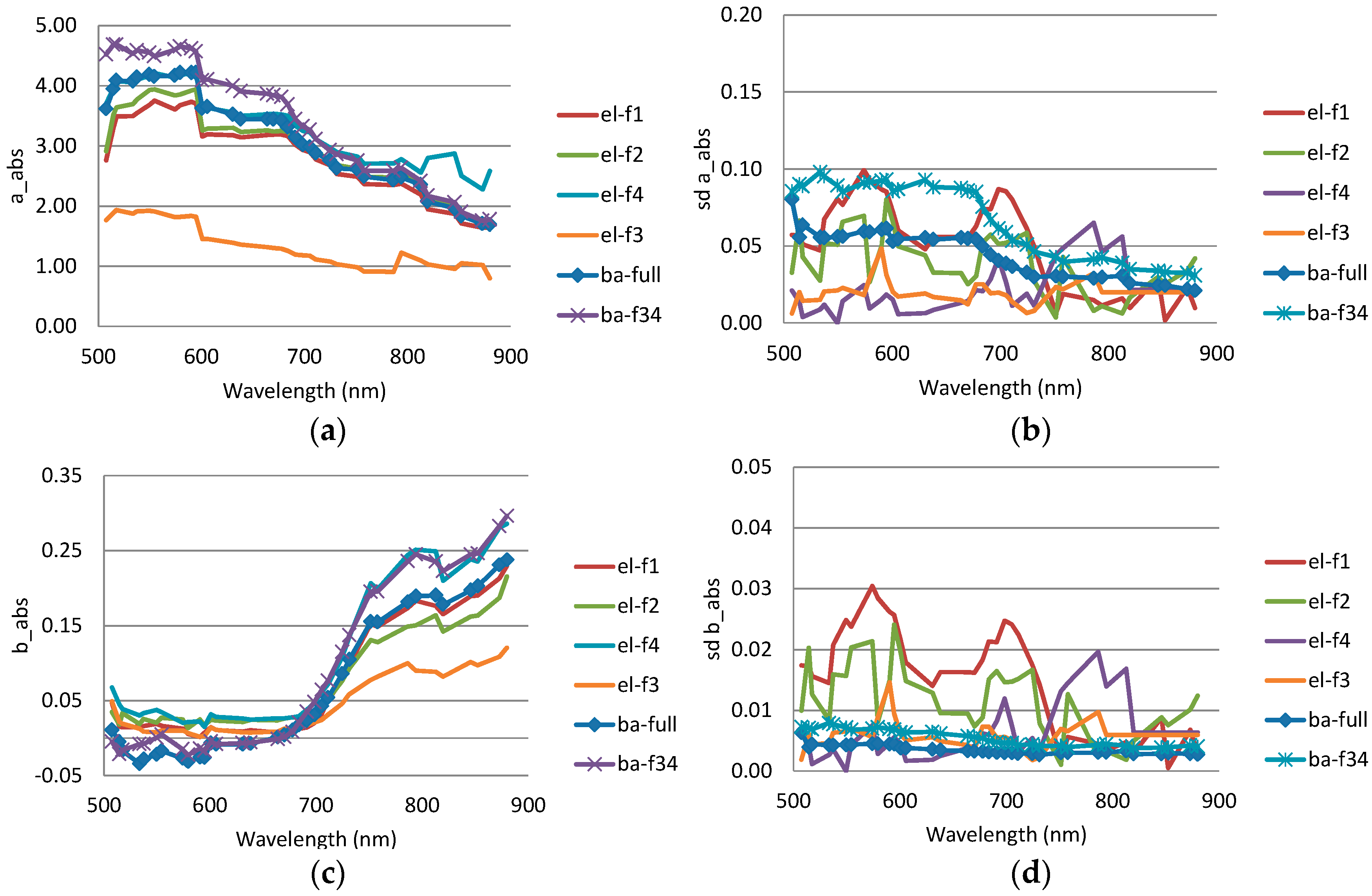
Figure 11.
(a) Estimated parameters and (b) their a posteriori standard deviations for green (L0 = 549.6 nm), red (L0 = 663.8 nm) and NIR (L0 = 794.0 nm) bands.
Figure 11.
(a) Estimated parameters and (b) their a posteriori standard deviations for green (L0 = 549.6 nm), red (L0 = 663.8 nm) and NIR (L0 = 794.0 nm) bands.
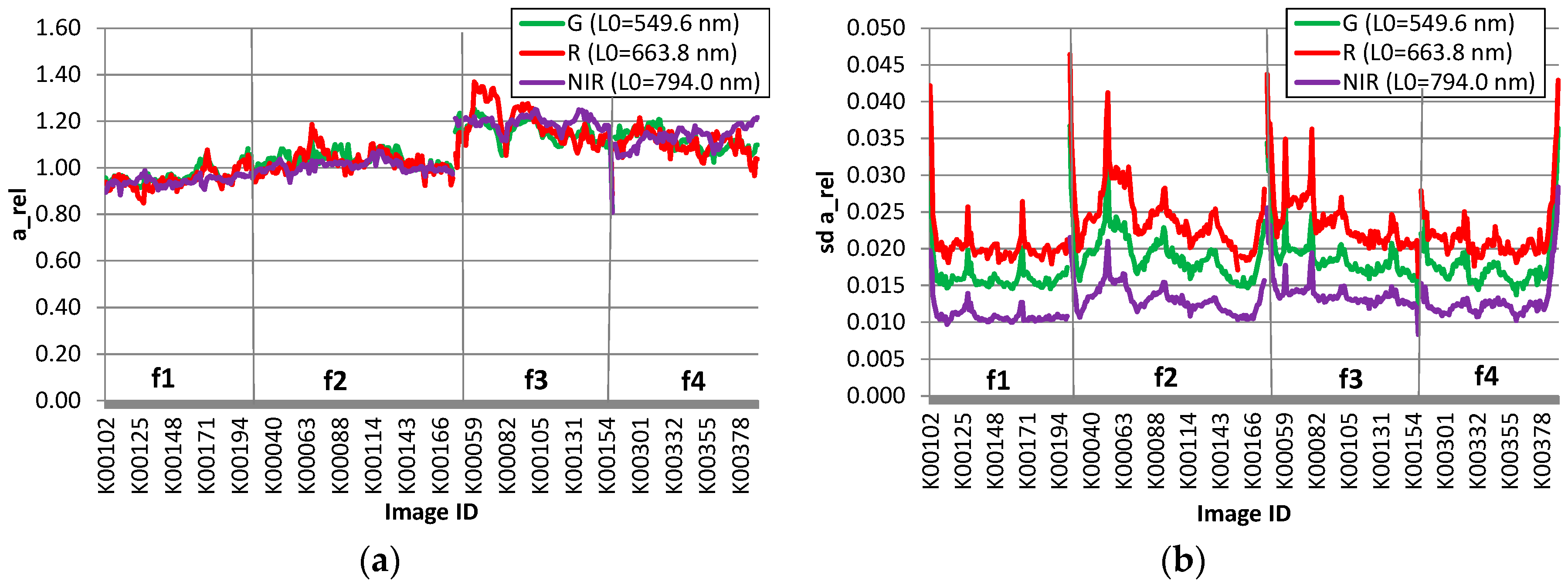
Figure 12.
Hemispherical directional reflectance factor (HDRF) plots created using the flight f34 data. (a) Raw HDRF observations; (b) anisotropy model and (c) BRDF corrected reflectance factors of green band; (d) Raw HDRF observations; (e) anisotropy model and (f) BRDF corrected reflectance factors of NIR band. In (b,e) the model is based on block adjustment.

Figure 13.
(a) BRDF parameters and (b) their standard deviations in the 4-parameter case for the full data; (c) BRDF parameters and (d) their standard deviations in the 2-parameter case for the flight f34.
Figure 13.
(a) BRDF parameters and (b) their standard deviations in the 4-parameter case for the full data; (c) BRDF parameters and (d) their standard deviations in the 2-parameter case for the flight f34.
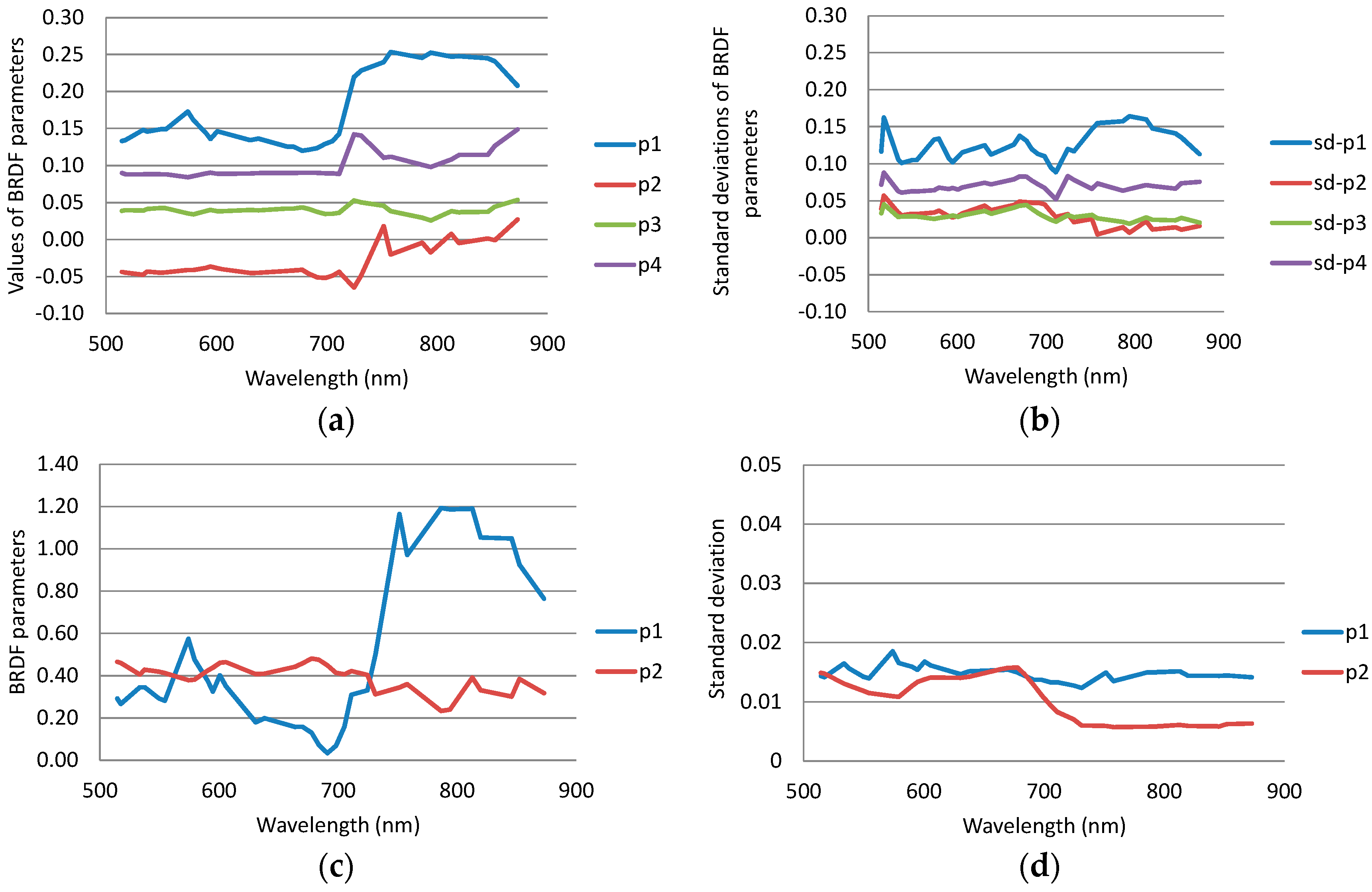
Figure 14.
Anisotropy factors for green (L0 = 549.6 nm), red (L0 = 663.8 nm) and NIR (L0 = 794.0 nm) bands in the solar principal plane for (a) the full dataset and (b) flight f34 with sun zenith angle of 39.8°.
Figure 14.
Anisotropy factors for green (L0 = 549.6 nm), red (L0 = 663.8 nm) and NIR (L0 = 794.0 nm) bands in the solar principal plane for (a) the full dataset and (b) flight f34 with sun zenith angle of 39.8°.

Figure 15.
Coefficient of variation (CV) for the (a) full dataset and (b) flight f34 dataset. nocorr: no radiometric correction; brdf-el: empirical line based reflectance transformation separately for each flight and BRDF correction; a_rel-brdf-el: empirical line based reflectance transformation separately for each flight and BRDF and relative image-wise correction; a_rel-brdf-abs: full radiometric block adjustment with absolute calibration and BRDF and relative image-wise correction.
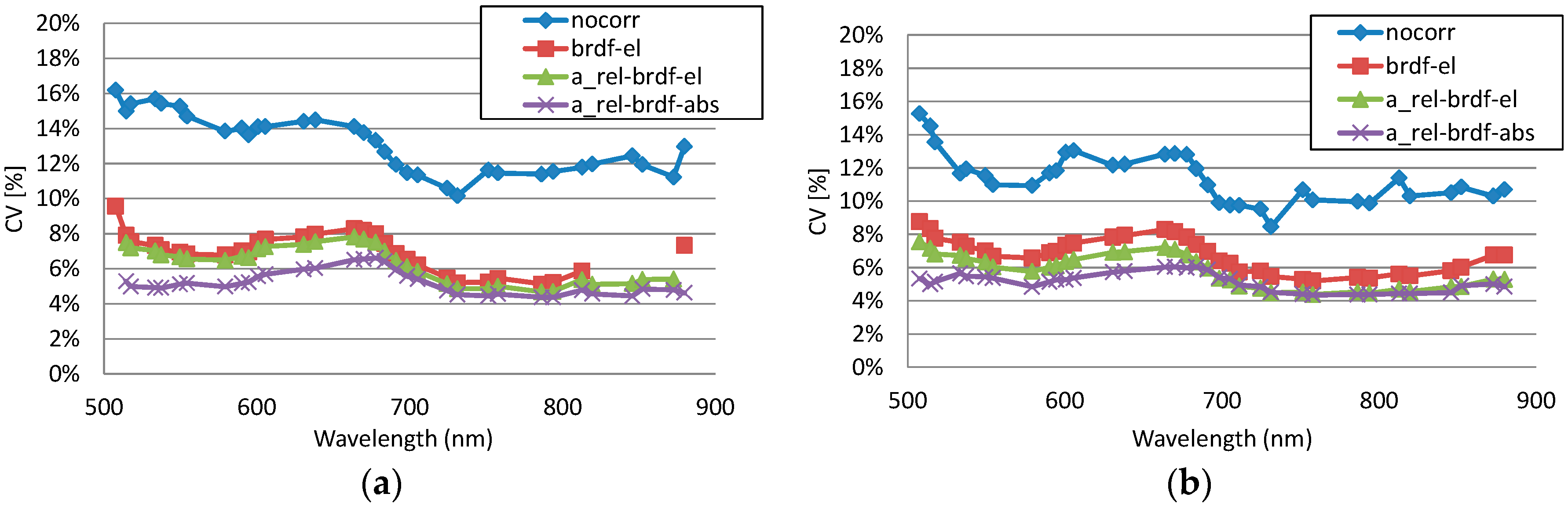
Figure 16.
Evaluation of quality of the mosaics using reflectance panels. (a) Spectra of white (W), grey (G) and black (B) reflectance panels; (b) RMSEs of residuals of panel spectra in corrected data with respect to the reference spectra for each panel. RCP: Radiometric control point; W-ref, B-ref and G-ref show the reference spectra measured in laboratory.

Figure 17.
Spectra sampled for selected soil (dry biomass < 53 g·m−2) and vegetation samples (dry biomass > 100 g·m−2) from the most nadir images; the legend shows the measured dry biomass as g·m−2 for each sample. (a) Full dataset with empirical line based reflectance calibration and no BRDF correction; (b) the full dataset and (c) the dataset with flights f34 with BRDF and relative corrections and the reflectance calibration.
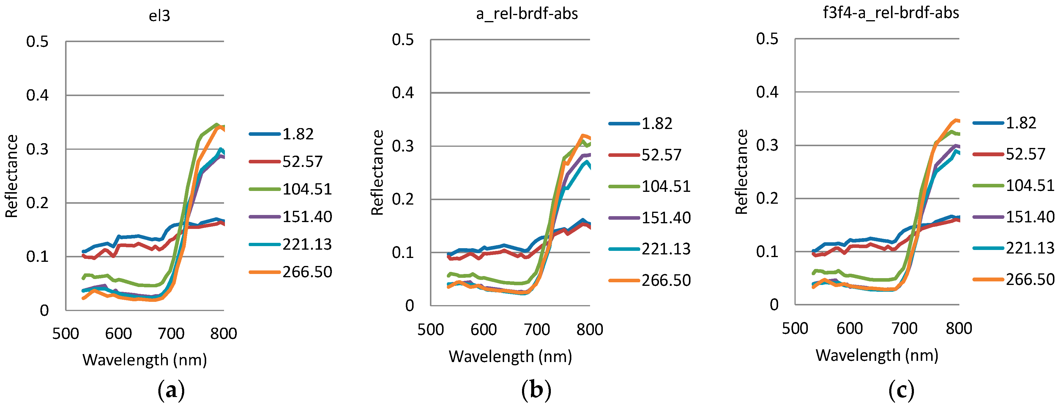
Figure 18.
Impact of radiometric processing in spectral values on multiple overlapping images. Reflectance spectra of vegetation sample 21 was observed in seven overlapping images; individual lines plotted with different colors represent spectra taken from the images. The radiometric processing options were as follows: (a) Full dataset with empirical line based reflectance calibration and no BRDF correction; (b) the full dataset and (c) the dataset with flight f34 with BRDF and relative image-wise corrections and the reflectance calibration.


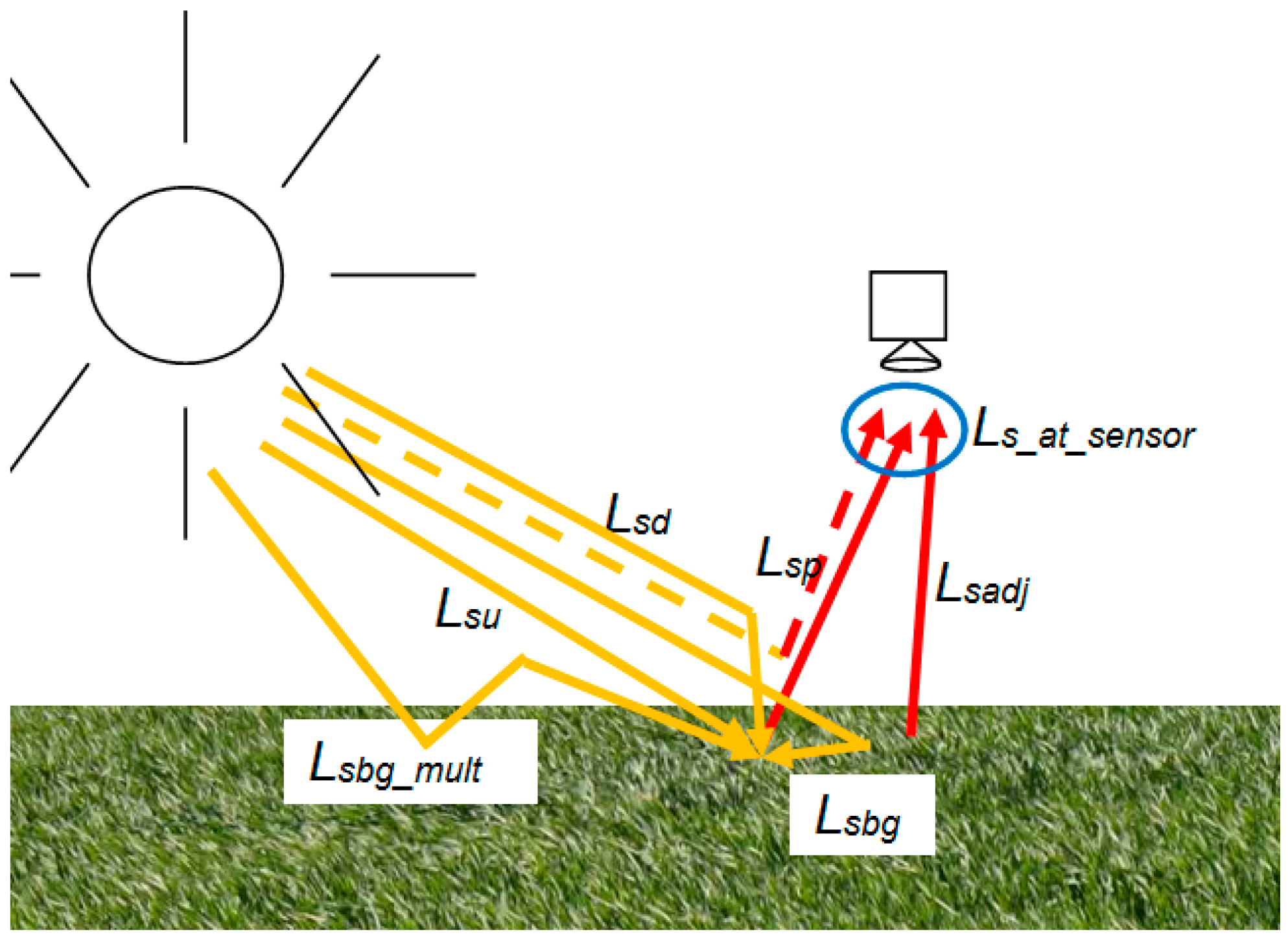
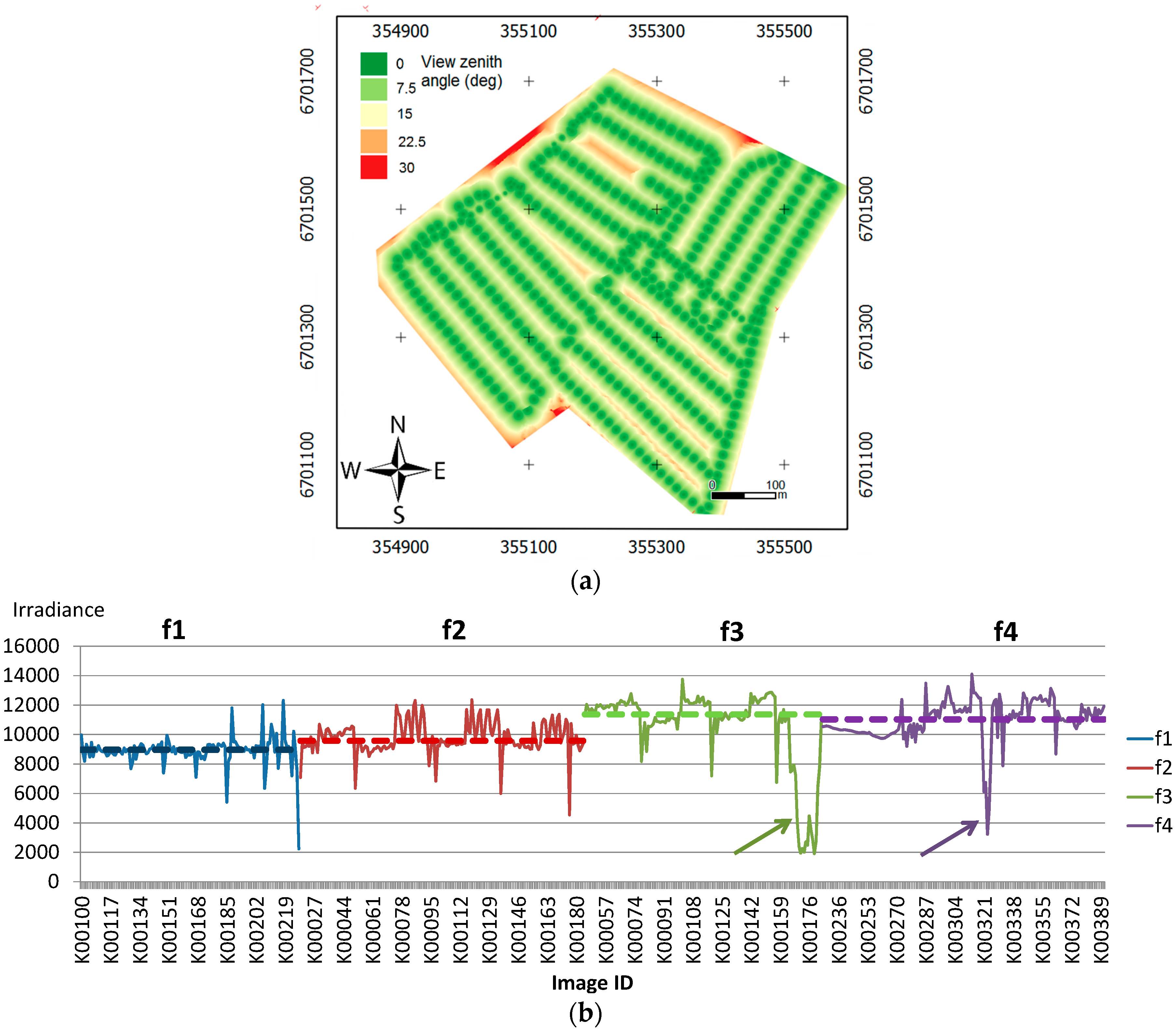
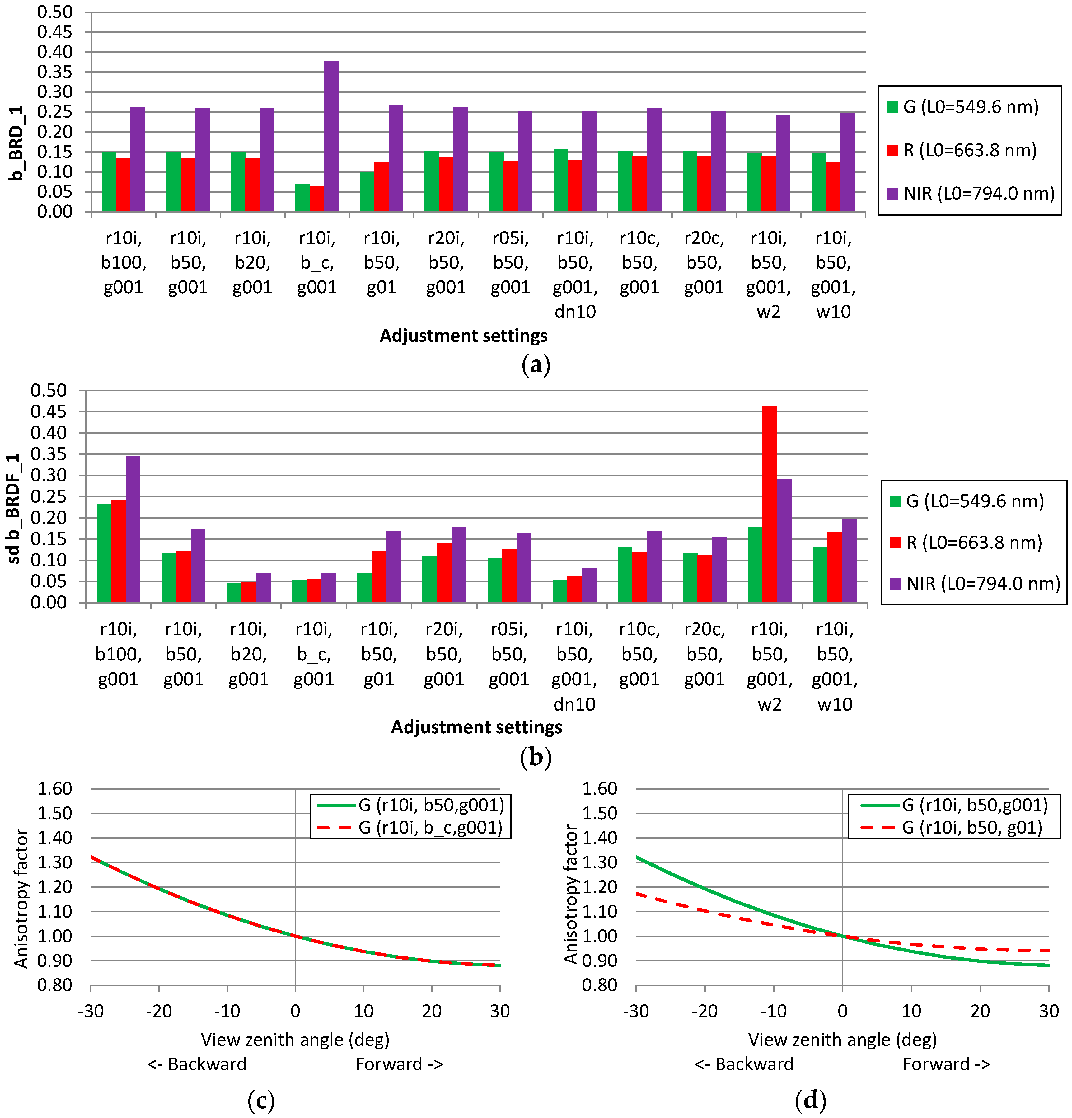
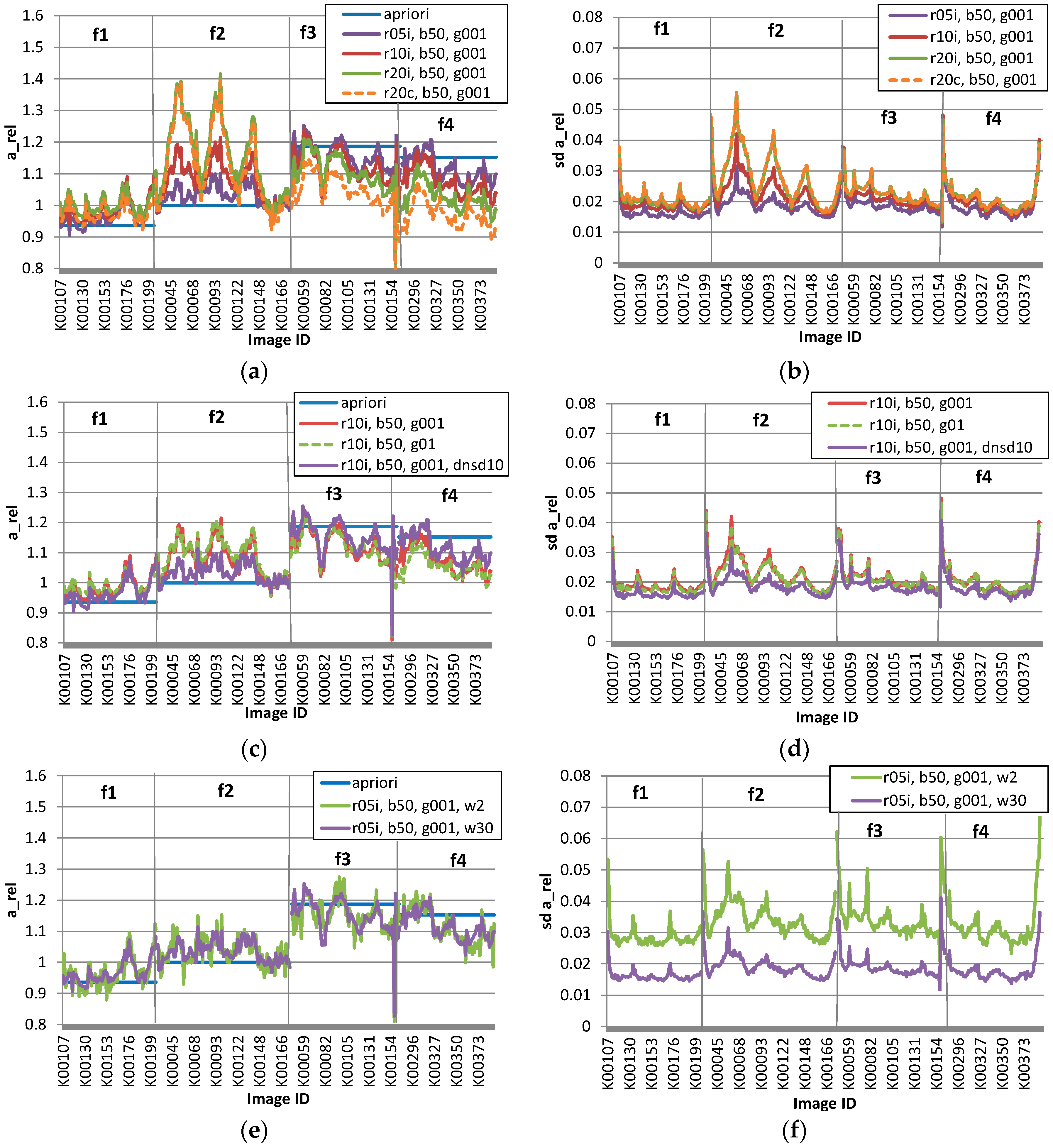
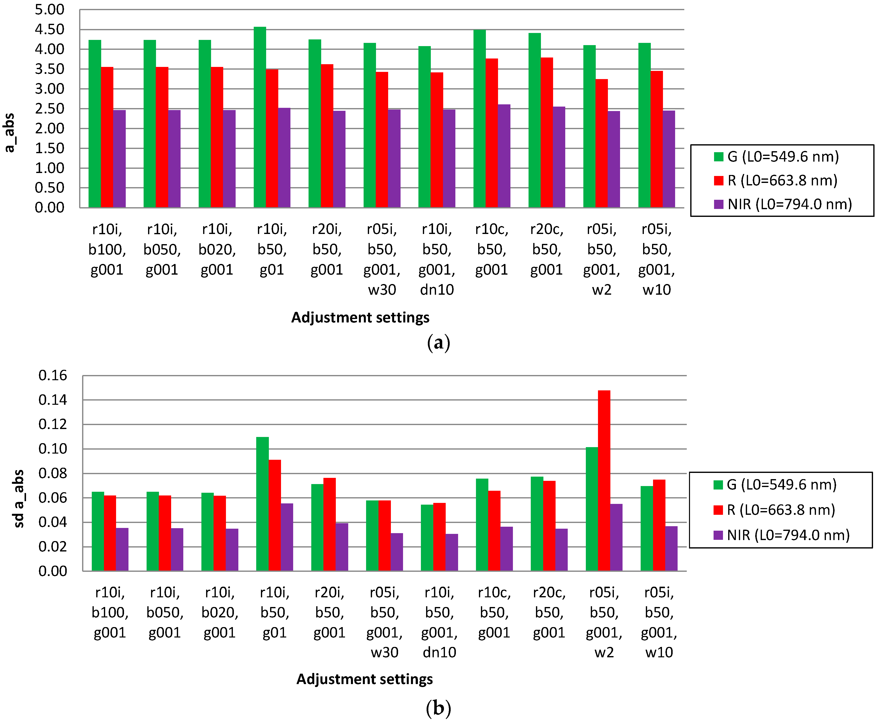
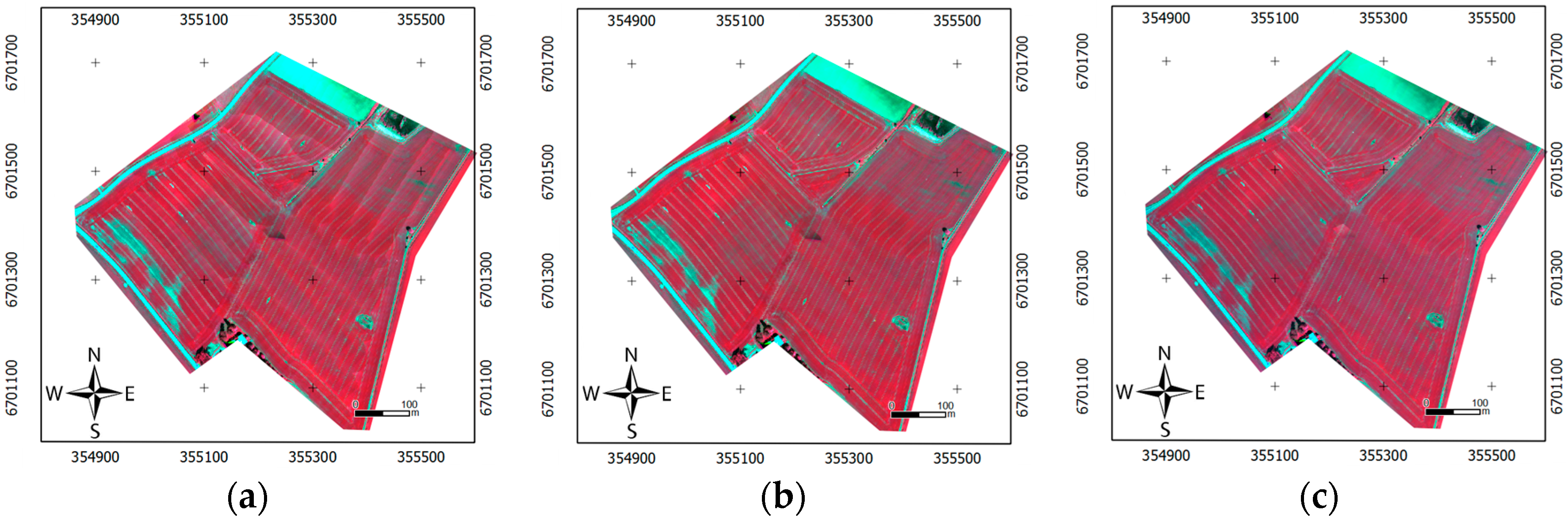
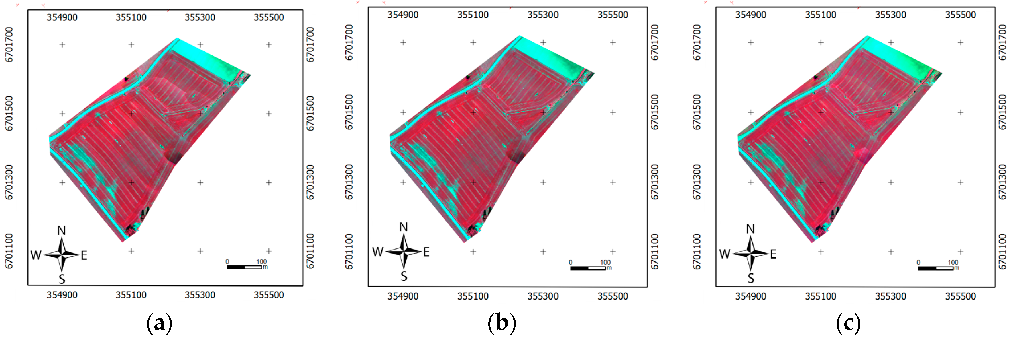
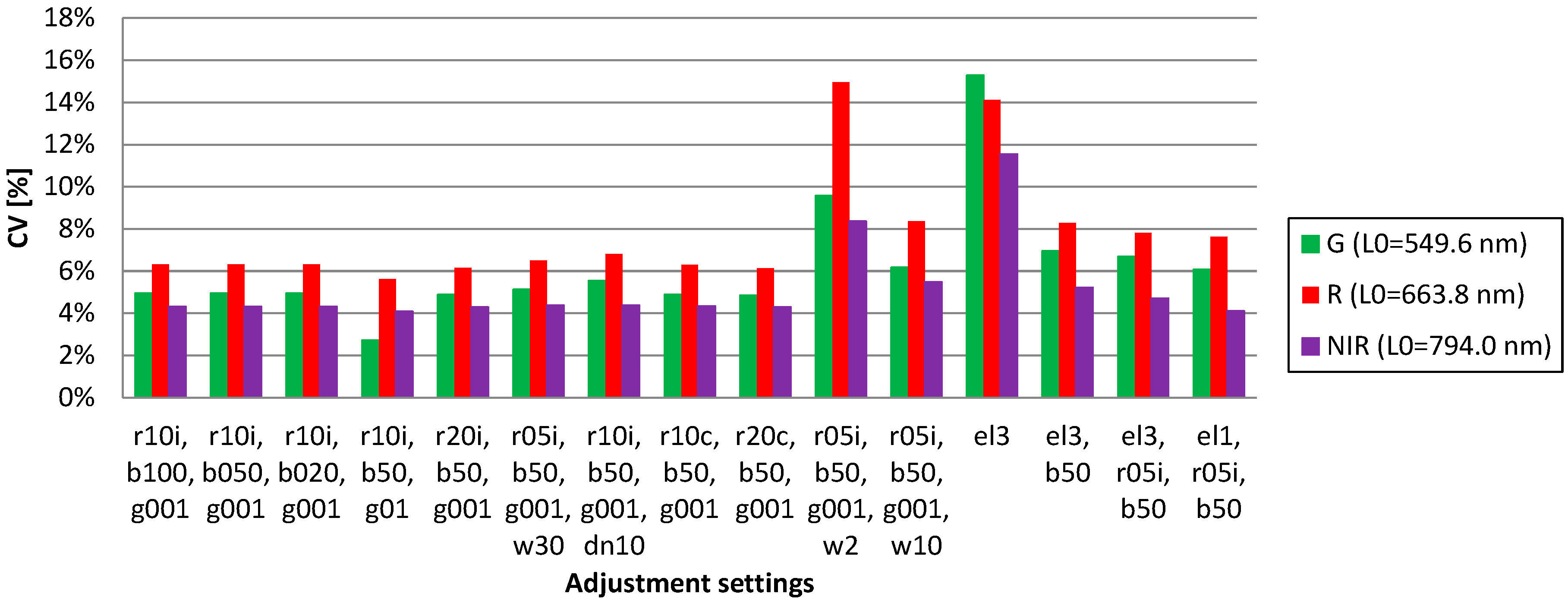
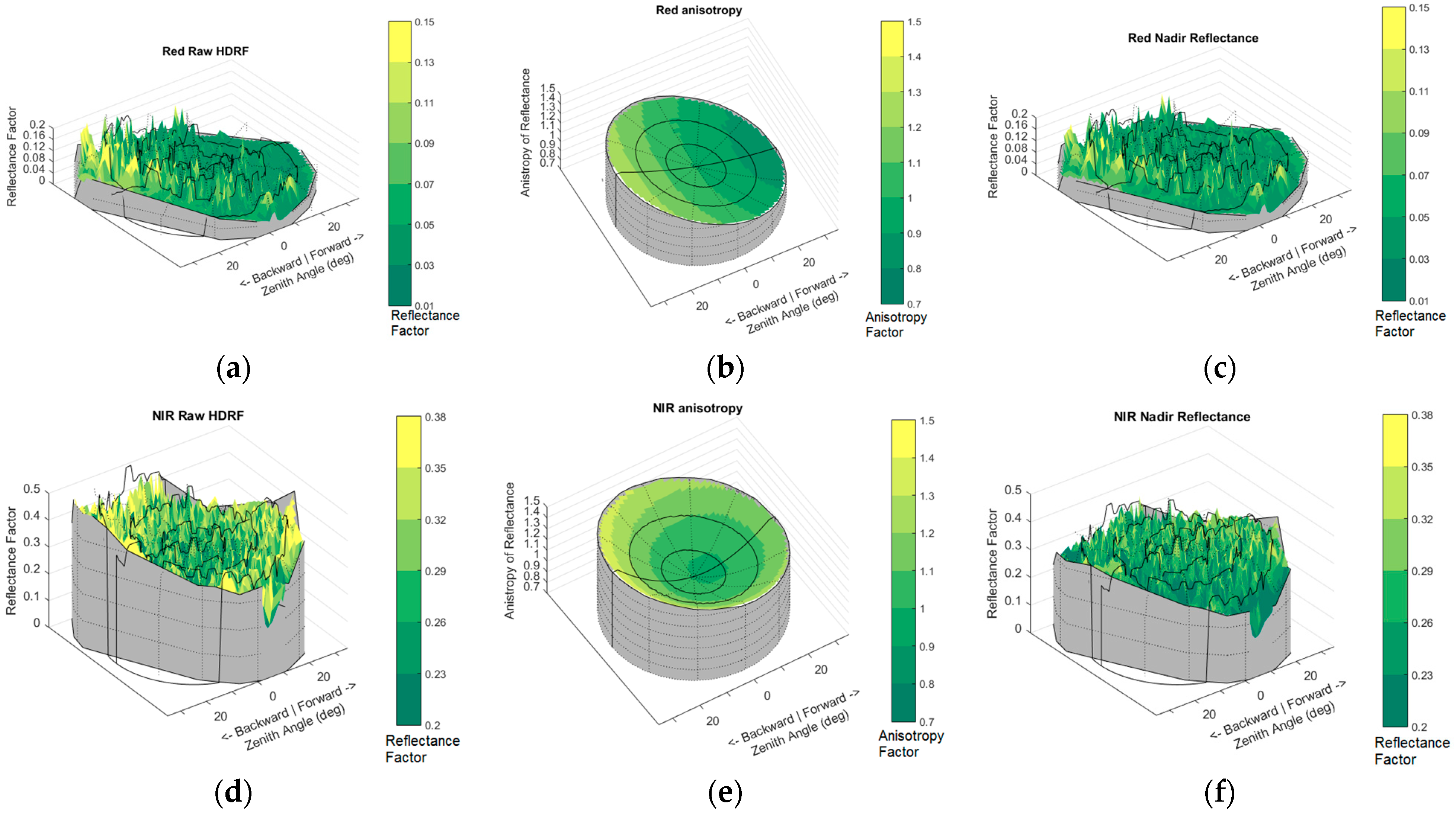
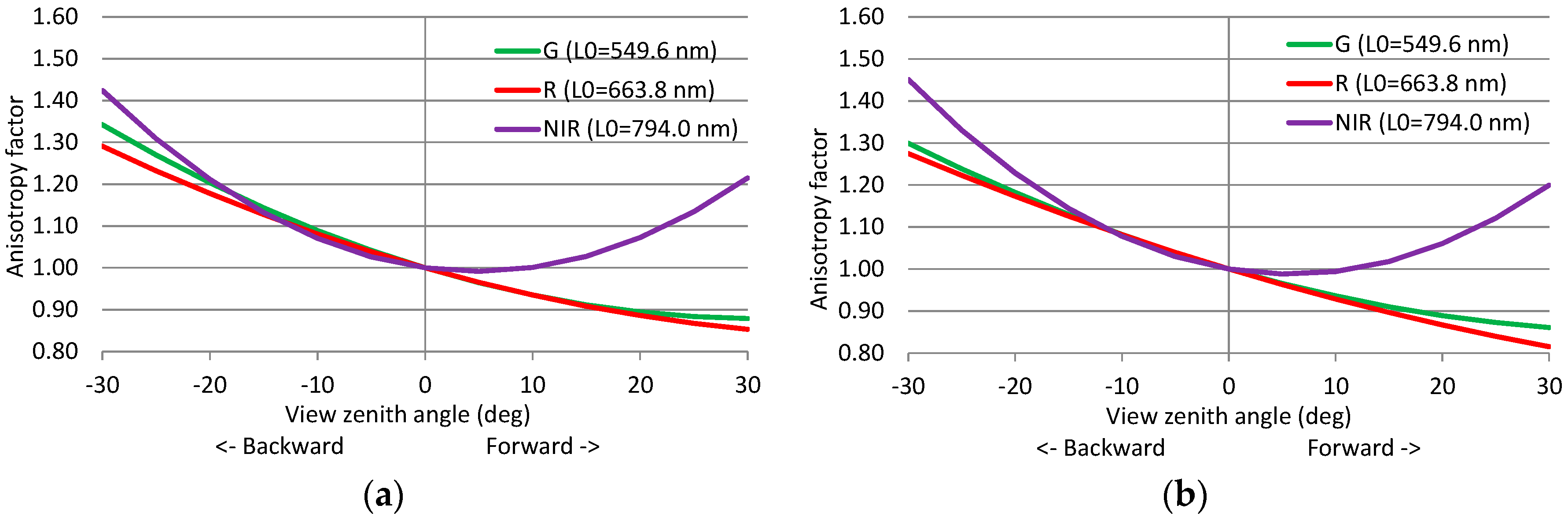
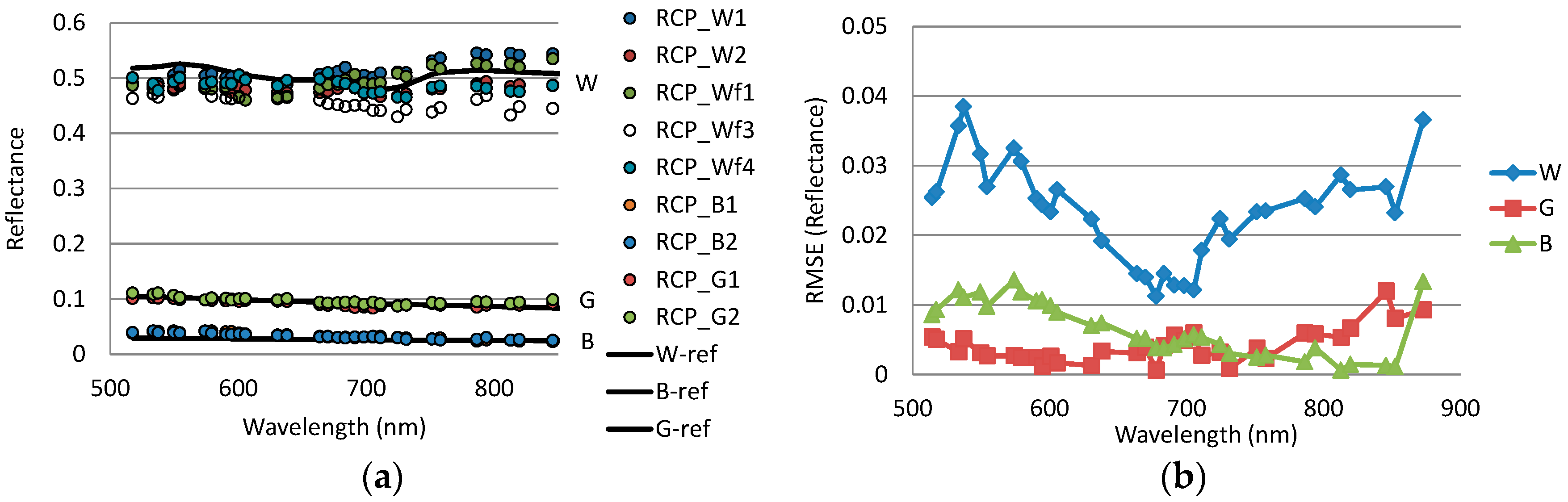
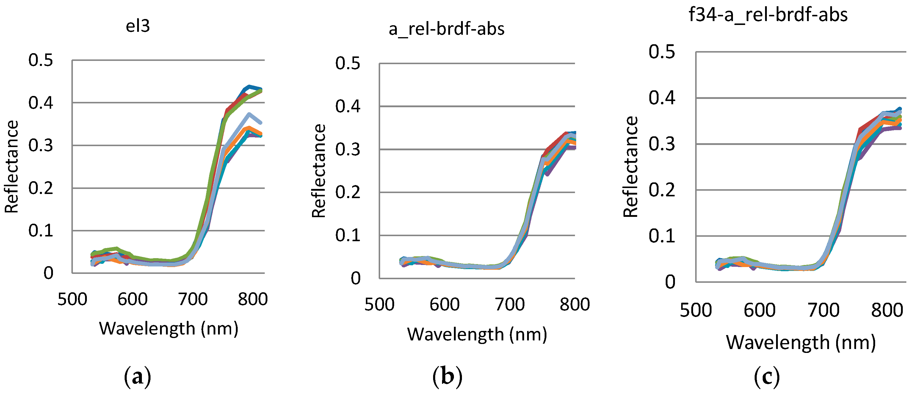
Table 1.
Spectral settings of the UAV hyperspectral camera.
| Central wavelength L0 (nm) | 507.60, 514.50, 517.50, 533.60, 537.40, 549.60, 554.40, 574.20, 579.30, 590.40, 594.70, 600.80, 605.70, 630.70, 638.20, 663.80, 670.10, 677.80, 683.70, 691.10, 698.40, 705.30, 711.10, 724.60, 731.30, 751.50, 757.90, 786.40, 794.00, 812.80, 819.70, 845.80, 852.30, 872.80, 879.90 |
| FWHM (nm) | 24.00, 20.00, 22.00, 24.00, 24.00, 24.00, 24.00, 24.00, 20.00, 22.00, 22.00, 32.00, 28.00, 32.00, 30.00, 32.00, 30.00, 28.00, 32.00, 32.00, 30.00, 28.00, 28.00, 30.00, 30.00, 28.00, 30.00, 30.00, 28.00, 30.00, 32.00, 30.00, 34.00, 32.00, 30.00 |
Table 2.
Characteristics of the image blocks. SunZen: Sun zenith angle; SunAz: Sun azimuth angle; FH: Flying height; GSD: Ground sample distance; p, q: Forward and side overlap, respectively.
Table 2.
Characteristics of the image blocks. SunZen: Sun zenith angle; SunAz: Sun azimuth angle; FH: Flying height; GSD: Ground sample distance; p, q: Forward and side overlap, respectively.
| Date, Flight | Time (UTC + 3) | Exposure (ms) | SunZen (°) | SunAz (°) | FH (m) | GSD (cm) | Overlaps p, q (%) |
|---|---|---|---|---|---|---|---|
| Flight 1 (f1) | 10:39–10:47 | 4 | 48.2 | 128.2 | 97.9 | 9.4 | 74, 60 |
| Flight 2 (f2) | 11:17–11:26 | 4 | 45 | 139.2 | 83.5 | 7.97 | 68, 51 |
| Flight 3 (f3) | 13:03–13:11 | 4 | 39.9 | 175.9 | 94.4 | 9.12 | 72, 60 |
| Flight 4 (f4) | 13:17–13:23 | 4 | 39.8 | 187.3 | 99.2 | 9.65 | 74, 60 |
Table 3.
Results of geometric processing by the PhotoScan. N adj ima: number of images used in the adjustment; N GCPs: number of GCPs; GSD: Ground Sample Distance; N pts/m2: number of points in m2 in the dense digital surface model.
Table 3.
Results of geometric processing by the PhotoScan. N adj ima: number of images used in the adjustment; N GCPs: number of GCPs; GSD: Ground Sample Distance; N pts/m2: number of points in m2 in the dense digital surface model.
| Flight number | Number of Cubes | N adj ima | N GCPs | GSD (cm) | N pts/m2 | Reprojection Error (pix) |
|---|---|---|---|---|---|---|
| Flight 1 | 128 | 426/384 | 5 | 9.4 | 113.177 | 0.419 |
| Flight 2 | 166 | 498/498 | 6 | 7.97 | 157.322 | 0.377 |
| Flight 3 | 139 | 414/414 | 7 | 9.12 | 120.24 | 0.39 |
| Flight 4 | 204 | 612/611 | 7 | 9.65 | 107.389 | 0.435 |
Table 4.
Parameter settings, number of parameters and number of observations used in calculations for different adjustment models. The cases 1–4 were calculated using the full blocks with all four flights and the cases 5–8 were calculated with the flight f34. : Number of relative image-wise correction unknowns; Bidirectional Reflectance Distribution Function (BRDF): number of BRDF unknowns; ,: number of reflectance calibration unknowns; EL: number of empirical line unknows; RTP: number of radiometric tie points; RTP-obs: number of radiometric tie point DN observations; RCP: number of reflectance panels.
| Case | BRDF | , | EL | RTP | RTP-obs | RCP | |
|---|---|---|---|---|---|---|---|
| (1) full, el3 | - | - | - | 3 × 2 | - | - | - |
| (2) full, brdf, el3 | - | 4 | - | 3 × 2 | 1426 | 10,303 | - |
| (3) full, , brdf, el3 | 451 | 4 | - | 3 × 2 | 1426 | 10,303 | - |
| (4) full, , brdf, abs | 451 | 4 | 2 | - | 1426 | 10,303 | 8 |
| (5) f34, el1 | - | - | - | 2 | - | - | - |
| (6) f34, brdf, el1 | - | 2 | - | 2 | 816 | 5252 | - |
| (7) f34, , brdf, el1 | 212 | 2 | - | 2 | 816 | 5252 | - |
| (8) f34, , brdf, abs | 212 | 2 | 2 | - | 816 | 5252 | 4 |
Table 5.
A priori values and standard deviations for the observations used in the calculations. : relative image-wise correction parameters; Irrad.: median irradiance observation; : standard deviations of ; : a priori values of the BRDF parameters; : standard deviations of the BRDF parameters 1,…, 4; p4_1: p4 settings for bands 1–23; p4_2: p4 settings for bands 24–35; : standard deviation of radiometric control point; : standard deviation of image observations.
| Case | a Priori | m: 1; 2; 3; 4_1/4_2 | m: 1; 2; 3; 4_1/4_2 | |||
|---|---|---|---|---|---|---|
| r10i,b50,g001 | Irrad. | 0.10 | 0; 0; 0; 0.1/0.2 | 0.25; 0.25; 0.25; 0.05/0.1 | 0.001 | 0.05 |
| r10i,b20,g001 | Irrad. | 0.10 | 0; 0; 0; 0.1/0.2 | 0.10; 0.10; 0.10; 0.02/0.04 | 0.001 | 0.05 |
| r10i,b100,g001 | Irrad. | 0.10 | 0; 0; 0; 0.1/0.2 | 0.50; 0.50; 0.50; 0.1/0.2 | 0.001 | 0.05 |
| r05i,b50,g001 | Irrad. | 0.05 | 0; 0; 0; 0.1/0.2 | 0.25; 0.25; 0.25; 0.05/0.1 | 0.001 | 0.05 |
| r10i,b_c,g001 | Irrad. | 0.10 | 0; 0; 0; 0.05/0.4 | 0.10; 0.10; 0.10; 0.025/0.05 | 0.001 | 0.05 |
| r20i,b50,g001 | Irrad. | 0.20 | 0; 0; 0; 0.1/0.2 | 0.25; 0.25; 0.25; 0.05/0.1 | 0.001 | 0.05 |
| r10i,b50,g01 | Irrad. | 0.10 | 0; 0; 0; 0.1/0.2 | 0.25; 0.25; 0.25; 0.05/0.1 | 0.01 | 0.05 |
| r10i,b50,g001,dn10 | Irrad. | 0.10 | 0; 0; 0; 0.1/0.2 | 0.25; 0.25; 0.25; 0.05/0.1 | 0.001 | 0.10 |
| r10c,b50,g001 | 1.0 | 0.10 | 0; 0; 0; 0.1/0.2 | 0.25; 0.25; 0.25; 0.05/0.1 | 0.001 | 0.05 |
| r20c,b50,g001 | 1.0 | 0.20 | 0; 0; 0; 0.1/0.2 | 0.25; 0.25; 0.25; 0.05/0.1 | 0.001 | 0.05 |
© 2018 by the authors. Licensee MDPI, Basel, Switzerland. This article is an open access article distributed under the terms and conditions of the Creative Commons Attribution (CC BY) license (http://creativecommons.org/licenses/by/4.0/).
Share and Cite
MDPI and ACS Style
Honkavaara, E.; Khoramshahi, E. Radiometric Correction of Close-Range Spectral Image Blocks Captured Using an Unmanned Aerial Vehicle with a Radiometric Block Adjustment. Remote Sens. 2018, 10, 256. https://doi.org/10.3390/rs10020256
AMA Style
Honkavaara E, Khoramshahi E. Radiometric Correction of Close-Range Spectral Image Blocks Captured Using an Unmanned Aerial Vehicle with a Radiometric Block Adjustment. Remote Sensing. 2018; 10(2):256. https://doi.org/10.3390/rs10020256
Chicago/Turabian StyleHonkavaara, Eija, and Ehsan Khoramshahi. 2018. "Radiometric Correction of Close-Range Spectral Image Blocks Captured Using an Unmanned Aerial Vehicle with a Radiometric Block Adjustment" Remote Sensing 10, no. 2: 256. https://doi.org/10.3390/rs10020256
Note that from the first issue of 2016, this journal uses article numbers instead of page numbers. See further details here.