Retrieval of Effective Correlation Length and Snow Water Equivalent from Radar and Passive Microwave Measurements

Abstract

Current methods for retrieving SWE (snow water equivalent) from space rely on passive microwave sensors. Observations are limited by poor spatial resolution, ambiguities related to separation of snow microstructural properties from the total snow mass, and signal saturation when snow is deep (~>80 cm). The use of SAR (Synthetic Aperture Radar) at suitable frequencies has been suggested as a potential observation method to overcome the coarse resolution of passive microwave sensors. Nevertheless, suitable sensors operating from space are, up to now, unavailable. Active microwave retrievals suffer, however, from the same difficulties as the passive case in separating impacts of scattering efficiency from those of snow mass. In this study, we explore the potential of applying active (radar) and passive (radiometer) microwave observations in tandem, by using a dataset of co-incident tower-based active and passive microwave observations and detailed in situ data from a test site in Northern Finland. The dataset spans four winter seasons with daily coverage. In order to quantify the temporal variability of snow microstructure, we derive an effective correlation length for the snowpack (treated as a single layer), which matches the simulated microwave response of a semi-empirical radiative transfer model to observations. This effective parameter is derived from radiometer and radar observations at different frequencies and frequency combinations (10.2, 13.3 and 16.7 GHz for radar; 10.65, 18.7 and 37 GHz for radiometer). Under dry snow conditions, correlations are found between the effective correlation length retrieved from active and passive measurements. Consequently, the derived effective correlation length from passive microwave observations is applied to parameterize the retrieval of SWE using radar, improving retrieval skill compared to a case with no prior knowledge of snow-scattering efficiency. The same concept can be applied to future radar satellite mission concepts focused on retrieving SWE, exploiting existing methods for retrieval of snow microstructural parameters, as employed within the ESA (European Space Agency) GlobSnow SWE product. Using radar alone, a seasonally optimized value of effective correlation length to parameterize retrievals of SWE was sufficient to provide an accuracy of <25 mm (unbiased) Root-Mean Square Error using certain frequency combinations. A temporally dynamic value, derived from e.g., physical snow models, is necessary to further improve retrieval skill, in particular for snow regimes with larger temporal variability in snow microstructure and a more pronounced layered structure.

1. Introduction

The mass of seasonal snow cover, or snow water equivalent (SWE) remains difficult to estimate on a global scale. Observational needs in terms of spatial resolution and product accuracy cannot be met by present satellite, in situ, or model-based data products at the global or regional-scale [1,2]. Global scale EO (Earth-Observation)-based products [3,4] rely on passive microwave sensors, while watershed-scale SWE has been successfully tracked with airborne LiDAR by relating observed snow height to the snow free DEM (Digital Elevation Model), and inferring SWE from the observations by modeling snow density [5]. The cost of timely airborne LiDAR surveys, however, is prohibitive for large-scale applications beyond individual watersheds or regions, so continuing efforts are made to apply Earth Observing satellite sensors for this purpose. Applying passive microwave observations from space for snow cover detection is appealing due to the availability of a long time series of daily observations with near global coverage, extending back almost 40 years. However, estimation of SWE has proved challenging despite several decades of efforts in developing retrieval approaches [6,7]. The main challenges hampering retrieval accuracy are related to the separation of the effect of increasing snow mass from other varying microstructural properties of the snowpack (density, layering, snow structural properties), and mitigating mixed pixel effects in the coarse scale passive microwave observations over heterogeneous landscapes. Existing active microwave sensors are unable to estimate SWE at the global scale and within user requirements because of the lack of current sensors at frequencies higher than X-band. In order to overcome these limits, a dual-band (X- and Ku) SAR mission called CoReH2O (Cold Regions Hydrology High-resolution Observatory, [8]), was proposed as a candidate for the 7th Earth Explorer mission of the European Agency (ESA), with the objective to provide SWE products at a spatial resolution of 200 m, exceeding that of current passive microwave methods. However, following phase-A CoReH2O was not selected for further development.

A priori characterization of snow structural parameters determining the scattering efficiency of microwaves in snow is of primary importance in the accuracy of SWE retrieval algorithms based on radiometer measurements, as this knowledge is required to resolve the total snow mass from observed signal changes [9,10,11]. A key parameter defining the scattering of microwaves has conventionally been the snow grain size, an estimate of the average size of snow grains in the snowpack [12]. The snow grain size has been used to empirically define the rate of microwave extinction in snow [13], which in turn has been applied in a radiative transfer model simulating emission from snow covered ground [14]. An effective grain size can be determined directly from passive microwave measurements, using widely available measurements from weather stations to fix the snow depth for the grain size inversion [15]; an effective grain size determined in this fashion can be related to grain sizes observed in the field [16]. Grain size estimates for application in SWE retrievals can also be obtained by means of applying a model to estimate snow grain metamorphism during the snow season [17].

The snow structural parameter itself remains difficult to measure, and the conversion from the 3D structure to effective model grain size is not unique due to the complex nature of snow grain metamorphism [18,19]. Theoretically-based emission and backscattering models based on the Dense Medium Radiative Transfer (DMRT) theory have assumed snow as a collection of spherical particles, introducing a stickiness parameter to emulate the sintering and clustering of snow grains [20,21,22]. However, it remains difficult to assign properties of snow observed in nature directly to these formulations of DMRT. While measurements of snow specific surface area (SSA) can be applied to estimate the snow optical grain diameter, empirical scaling is required to translate this value to one explaining the observed microwave response [23]. Recent efforts have focused on simulating snow as a bicontinuous medium, simulating the resulting active and passive microwave response with some success [24]. Arguably, statistical parameters such as autocorrelation length of the snow structure in different axial directions are able to describe the snow microstructure with higher fidelity than the conventional measure of grain size [25].

An effective grain size can be used to approximate the scattering behavior of the snowpack using a forward model based on that parameter [15,16]. The term ‘effective’ refers to the fact that the grain size may compensate for simplifications in the model setup (namely the aggregation of a multiple-layered snowpack to a single layer, a practical implementation for operational SWE retrieval schemes, including the one envisaged for CoReH2O), as well as other deficiencies in model input data or model physics. In this study, we present the retrieval of an effective correlation length, which similarly describes the radiative transfer properties of snow by a single parameter. The effective correlation length is retrieved from active and passive microwave observations of naturally accumulated snow over four winter seasons at a test site in northern Finland. We examine the interchangeability of the retrieved correlation length (derived independently from active and passive measurements at different frequencies) for the purpose of initializing the retrieval of SWE from radar observations. Specifically, the study has the following objectives;

• Retrieve an effective snow correlation length by matching emission and backscattering model predictions to the radiometer and radar measurements, respectively. Examine the seasonal behavior in the observed changes and relate these to physical properties of the snowpack
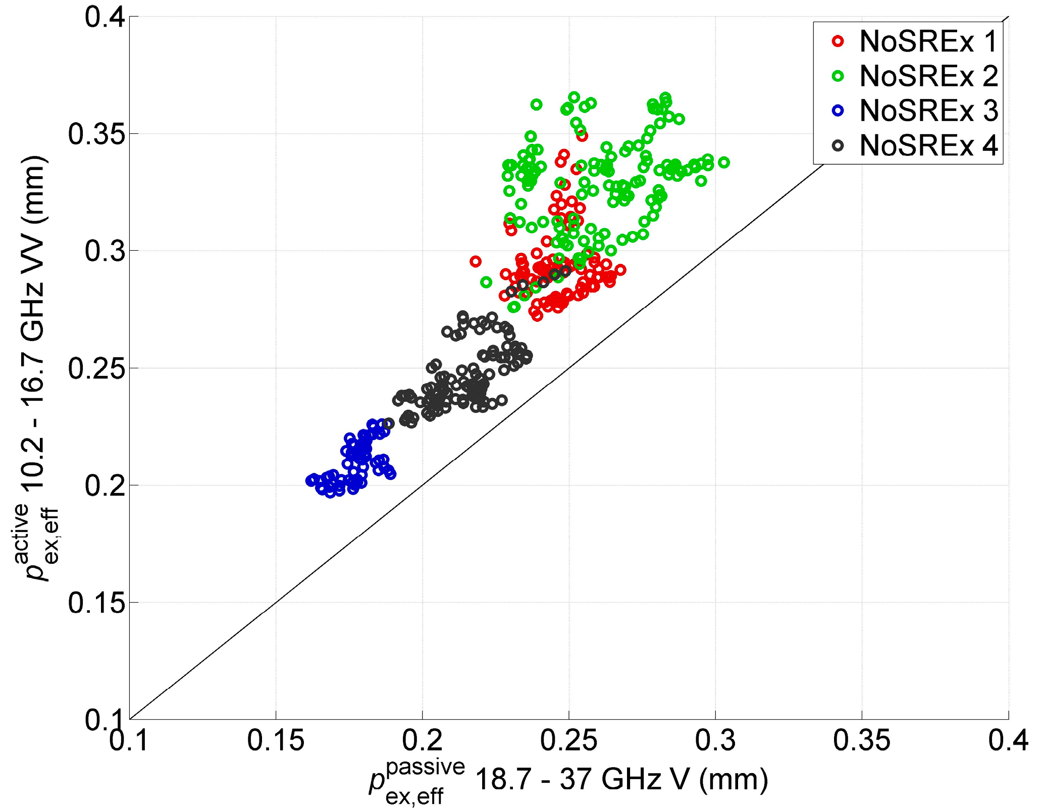
• Examine the interchangeability of the active and passive microwave effective correlation length, and determine the sensitivity of these estimates to observation frequency and polarization.
• Apply an effective correlation length derived from one sensor type (passive) to initialize the retrieval of SWE using the other (active). Compare the impact on SWE retrievals of applying temporally dynamic effective correlation length versus a seasonally constant value, optimized separately for each winter season.

The third objective is meant as a first feasibility demonstration of synergistic active/passive retrieval methods for potential implementation in proposed satellite mission concepts exploiting co-incident radar and radiometer measurements [26].

The study makes use of data acquired from the NoSREx (Nordic Snow Radar Experiment, [27]). The experiment was initiated in November 2009 in support of CoReH2O geophysical algorithm development and included observations of a boreal forest snowpack using both active and passive microwave instruments over four winter seasons.

Section 2 of the study describes the forward model and the methods applied for retrieval of correlation length, and SWE. Section 3 presents the NoSREx datasets. Section 4 presents the main results of the study. These are discussed and the conclusions of the study are given in Section 5.

2. Forward Model and Retrieval Method

2.1. MEMLS3&a Model

The Microwave Emission Model for Layered Snowpacks (MEMLS, [28,29]) is a semi-empirical model utilizing snow correlation length (i.e., the autocorrelation of snow structural variations in a spatial dimension) to define snow microstructure. This can be related to snow-scattering parameters better than the ambiguous snow grain size [25], and is also a parameter that can be objectively estimated from field and laboratory observations. A recent modification to MEMLS expanded the model to also simulate microwave backscattering from snow (MEMLS3&a, [30]). MEMLS3&a allows, by means of model inversion, determination of an effective correlation length describing the average scattering properties of a snowpack using a unified physical approach for both active and passive microwave observations.

The original MEMLS model considers snow as a vertically stacked system of homogeneous snow layers, with each layer characterized by temperature, thickness, liquid water content, salinity, density and correlation length. Radiative transfer in individual layers is calculated using a two-flux approach (fluxes propagating in forward and backward directions), while scattering and absorption coefficients are functions of a six-flux model (including fluxes in perpendicular directions). The absorption coefficient is obtained from density, frequency, temperature, moisture and salinity; the scattering coefficient is determined based on frequency, density, and correlation length. Several empirical formulations have been derived to relate correlation length with the six-flux scattering coefficient [28]; MEMLS also includes an option to use the Improved Born Approximation (IBA) to estimate correlation length, expanding the model for coarse-grained snow [29]. For multiple layers, a sandwich model is applied to determine the effects of internal scattering and reflections at layer interfaces. In the MEMLS3&a model, a prediction of backscattering from snow is calculated based on the specular and diffuse components of snow reflectivity. The specular component is determined from a mean-square slope of slight surface undulations, assuming a Gaussian distribution. The diffuse component is determined from the diffuse component of the total snow reflectivity, which in turn is related to the total emissivity of the snowpack [30].

2.2. Retrieval of Effective Correlation Length

MEMLS3&a was applied in a one-layer configuration to retrieve effective exponential correlation length p_ex,eff (i.e., a value of correlation length matching model predictions to observations). The approach is analogous to the method introduced by Pulliainen [15] for large-scale passive microwave data using conventional snow grain size. The cost function for iterative inversion can be formulated as

$$CF\left(p_{\mathrm{ex},\mathrm{eff}}\right)={\displaystyle \sum }_{k=1}^P\frac{{\left[{\mathrm{\Phi }}_k^s\left(p_{\mathrm{ex},\mathrm{eff}},SD,x_1,\dots ,x_n\right)-{\varphi }_k^s\right]}^2}{{\sigma }_k^s}$$

(1)

where SD is the snow depth, p_ex,eff the effective (exponential) correlation length, P the number of observation channels k, ${\mathrm{\Phi }}_k^s$ the forward model estimate for sensor types (active or passive), x_n the model parameters excluding SD and p_ex,eff, ${\varphi }_k^s$ the observed microwave response and ${\sigma }_k^s$ the variance of the combined error of the sensor and the forward model. The same a priori parameters x were applied in both active and passive forward model simulations. The Improved Born Approximation (IBA) was applied to calculate the snow-scattering coefficient [29]. Ground reflectivity (s0v, s0h) at different frequencies corresponds to bare soil with a surface roughness (h_rms) of 1 cm and a ground permittivity (ε_gnd) of 4, calculated using an empirical model [31]. The specular part of reflectivity in MEMLS was considered to be 0.9 across all frequencies. Downwelling sky brightness temperature was estimated using a 55% fractile atmosphere transmissivity model [32]. Snow density (ρ_snow) was assigned a constant value of 200 kg m⁻³, which closely corresponds to the approximate bulk density over the four seasons at the test site [27], and which is also very close to the typical taiga snow density [33]. SD was taken from measured in situ snow depth, and was in baseline retrievals the only temporally variable ancillary input. All other parameters were kept as constants, while p_ex,eff was the sole free parameter in the iterative optimization (minimization) of F. It should be noted that this approach was chosen as the baseline, although measured values for factors such as air temperature (T_air), ground temperature (T_gnd), ground permittivity and snow density would have been available from the NoSREx experiment. However, our purpose was to emulate potential satellite scale retrievals, where such values are likely not widely available. The retrieved effective correlation length thus accounts also for potential errors arising from the use of these constant ancillary parameters.

The retrievals of effective correlation length using active and passive microwave observations are henceforth labeled p^active_ex,eff and p^passive_ex,eff, respectively. The ancillary parameters x, as well as other setting of MEMLS3&a, are summarized in

Table 1. Ancillary input parameters and MEMLS3&a model settings.

Parameter	Description	Value
F	Centre frequency	active: 10.2, 13.3, 16.7 GHz passive: 18.7, 37 GHz
θk	Incidence angle	50°
s0v	V-pol reflectivity of snow-ground interface	0.03(@37 GHz)…0.06(@10.2 GHz) using εgnd = 4 and hrms = 1 cm [31]
s0h	H-pol reflectivity of snow-ground interface	0.05(@37 GHz)…0.07(@10.2 GHz) using εgnd = 4 and hrms = 1 cm [31]
ss0v, ss0h	Specular part of reflectivity	0.9
q	Fraction of cross-polarized scattering	(cross polarization not used)
Tsky	Downwelling sky brightness temperature	5 (@10.2 GHz) to 35 K (@37 GHz) [32]
Tgnd	Ground temperature	−5 °C
Tsnow	Snow temperature	−5 °C
ρsnow	Snow density	200 kg m−3
Scattering model		IBA
Number of layers		1

.

To analyze the effect of uncertainties of the approach, retrievals of p^active_ex,eff and p^passive_ex,eff were repeated using measured values for available ancillary parameters for T_air, T_gnd, ε_gnd and ρ_snow. T_air, T_gnd and ε_gnd were taken from automated sensors. The ground reflectivity was recalculated based on the measured ε_gnd, considering the measured value valid across all frequencies, which is a reasonable assumption for frozen ground [34]. The measured density was taken from weekly manual observations of bulk snow density (measurements were made twice a week for the first season of NoSREx). To reduce random variability due to variable location of the manual measurements, and to obtain an estimate for each day, a third order fit was performed on the density data, using the fitted values in retrievals.

2.3. Retrieval of SWE

SWE was determined iteratively from active and passive microwave measurements by inverting the MEMLS3&a model. The cost function used in iterative minimization is analogous to Equation (1), so that

$$CF\left(\mathrm{SWE}\right)={\displaystyle \sum }_{k=1}^P\frac{{\left[{\mathrm{\Phi }}_k^s\left(p_{\mathrm{ex},\mathrm{eff}},\mathrm{SWE},x_1,\dots ,x_n\right)-{\varphi }_k^s\right]}^2}{{\sigma }_k^s}$$

(2)

where SWE is the sole free parameter and p_ex,eff is given a priori. The SWE retrieval tests in this study were made using radar backscattering observations; four configurations (labeled Configurations 1 to 4) were used to initialize p_ex,eff in the retrieval:

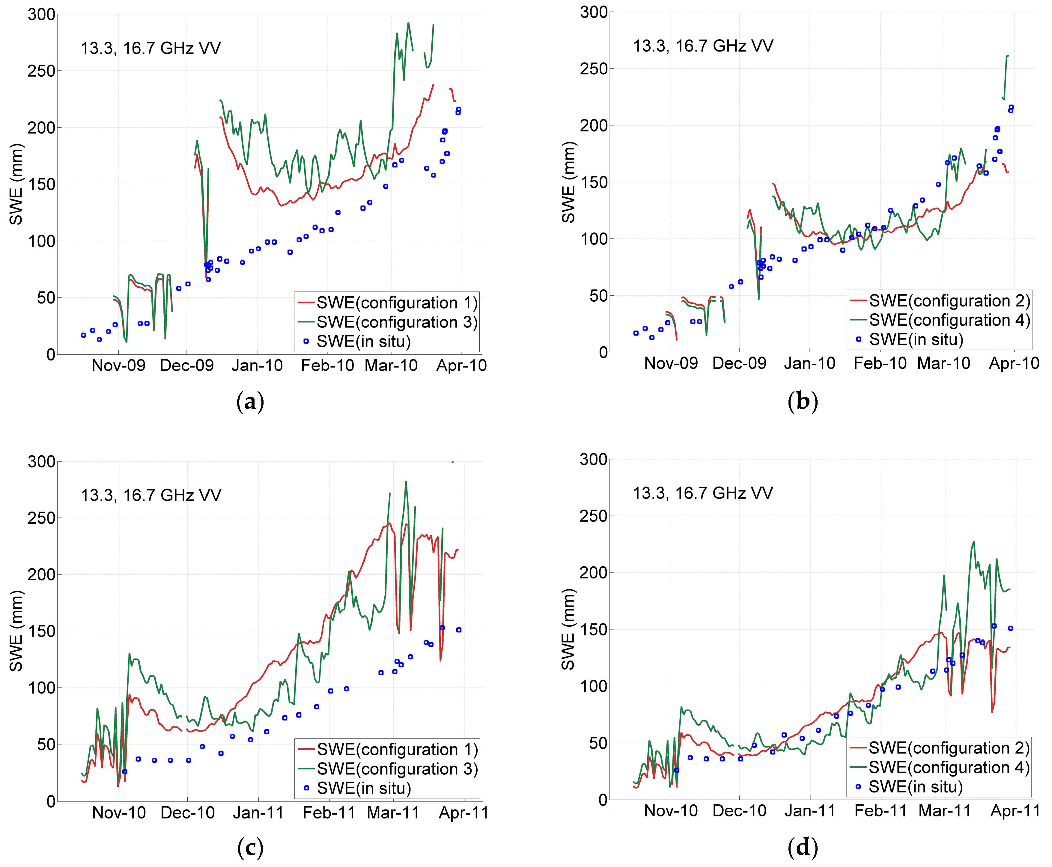
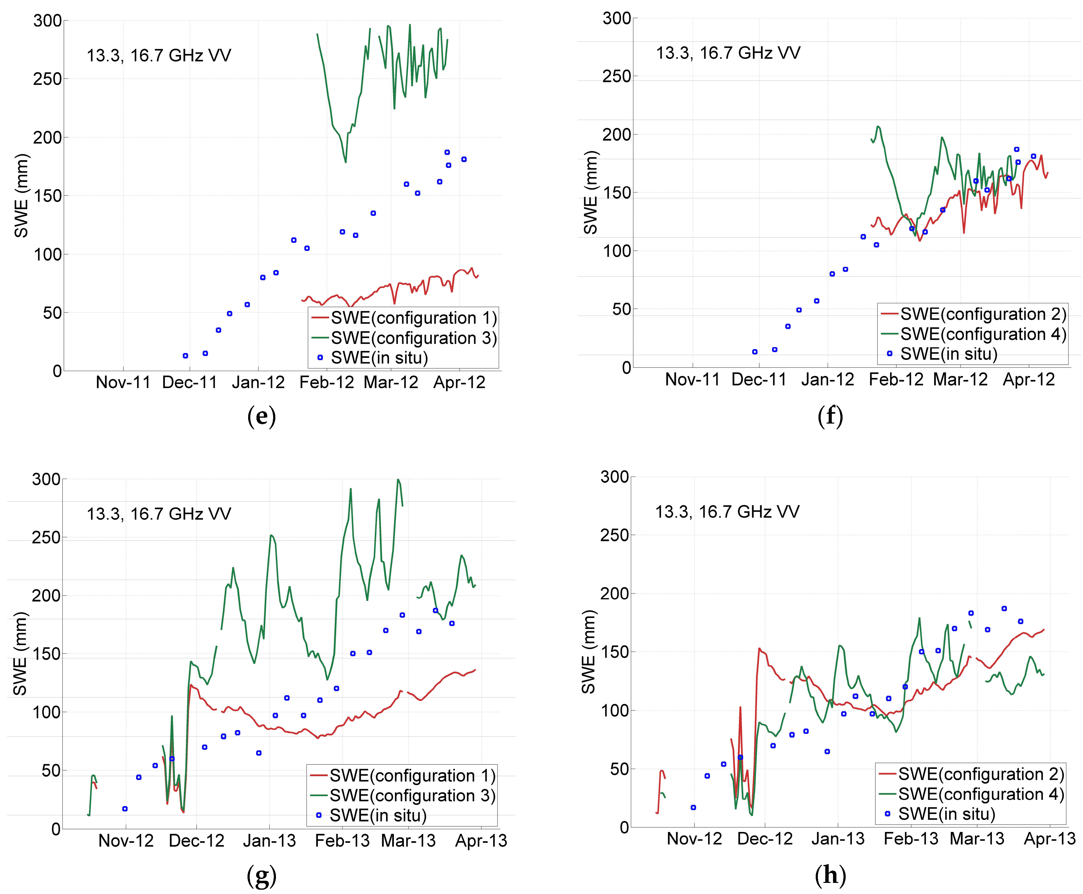
• Configuration 1: An overall average of optimized daily values <p^active_ex,eff> was calculated from all retrievals of p^active_ex,eff under dry snow conditions for all four seasons. Averages were calculated separately for each channel and combination. These average values of optimizations were used to initialize the respective retrievals of SWE at time t (p_ex,eff (t) = <p^active_ex,eff>).
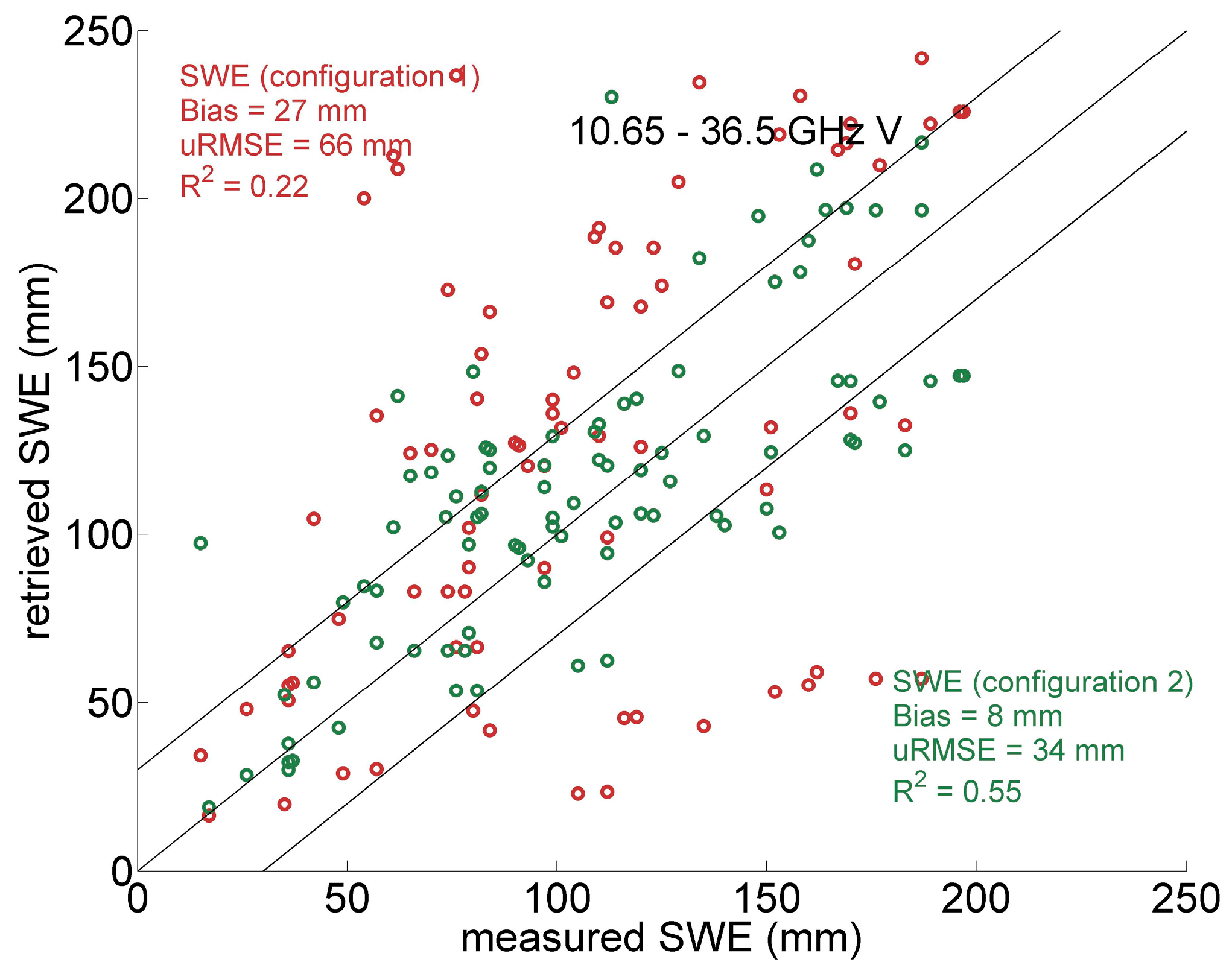
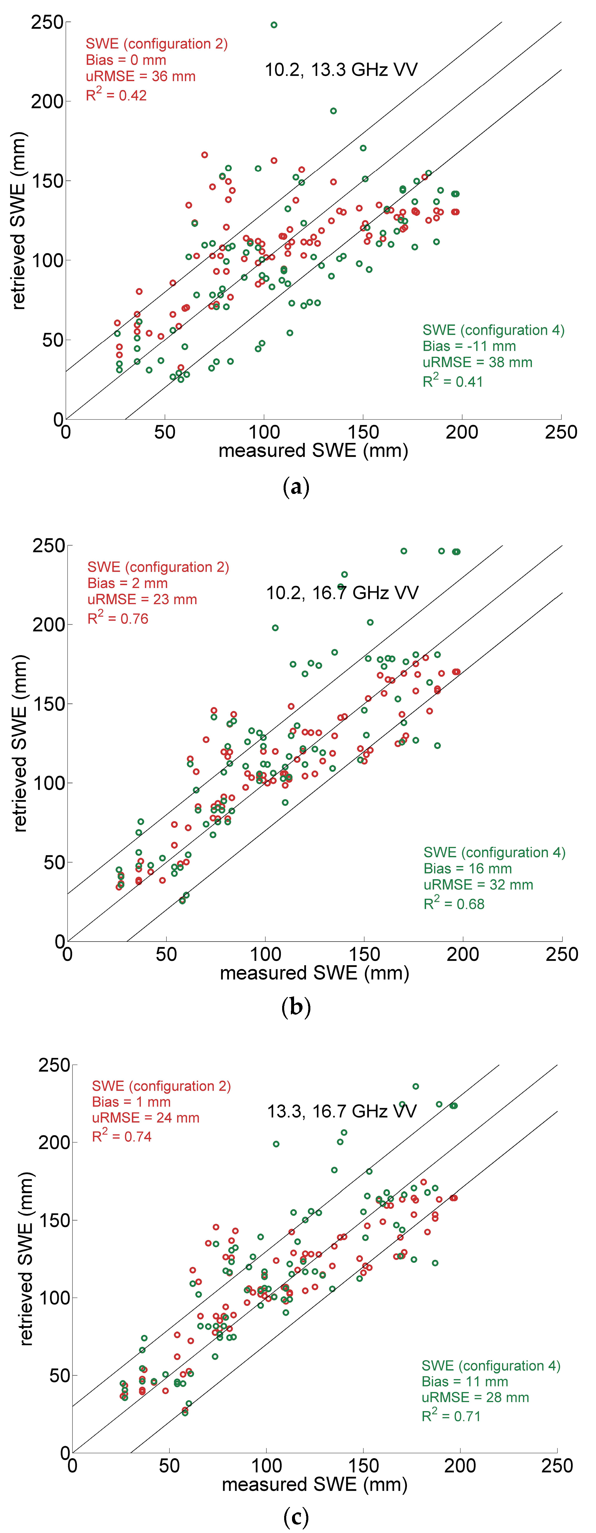
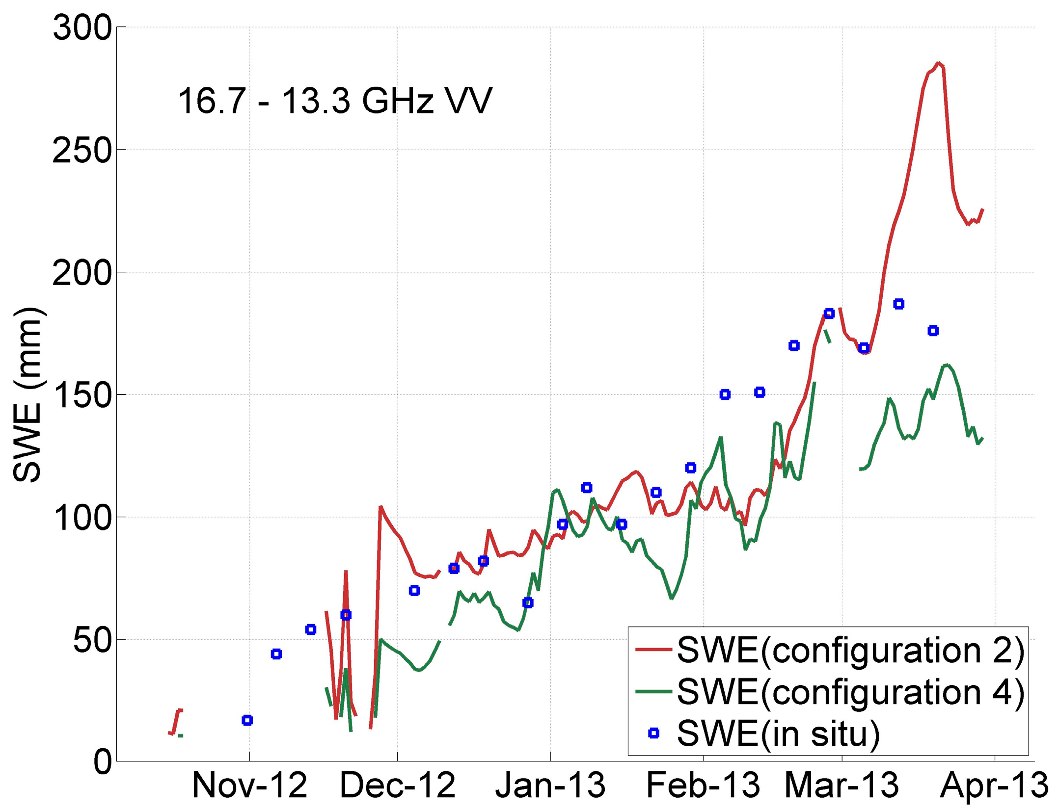
• Configuration 2: As in Configuration 1, but the average of optimized daily values <p^active_ex,eff> was calculated and applied in SWE retrieval individually for each of the four winter seasons, thus applying seasonal optimization to the retrieval.
• Configuration 3: For each radar retrieval of SWE at time t, the effective correlation length was acquired from the temporally closest passive microwave retrieval (p_ex,eff (t) = p^passive_ex,eff (t)). As a default, p^passive_ex,eff was obtained from 18.7–37 GHz, V-pol, radiometer retrievals.
• Configuration 4: As in Configuration 3, but the value of p^passive_ex,eff was scaled so that p_ex,eff (t) = β p^passive_ex,eff (t). A constant scaling value β was applied in SWE retrieval across all seasons.

The first of the above configurations represents a baseline retrieval where p_ex,eff is optimized for the site in question based on a climatological average, but without any seasonal sensitivity to potential changes. The second configuration emulates a retrieval where p^active_ex,eff has been seasonally optimized, but otherwise kept temporally constant. In practice, this could be achieved e.g., by means of applying e.g., a physical snow model. The contrast with Configuration 1 thus demonstrates the effect of using a seasonally sensitive microstructural indicator, compared to a static climatological average. The third and fourth configurations emulate a scheme where the active microwave retrieval is initialized using effective correlation length derived from passive microwave observations, with the last configuration applying an additional scaling factor, to account for the mean difference in the retrieved p^active_ex,eff and p^passive_ex,eff. All other input variables of the MEMLS3&a model were kept constant in the retrieval, following Table 1, as in the retrieval of p_ex,eff.

As with retrievals of p_ex,eff (see Section 2.2), SWE retrievals were repeated using measured ancillary data for T_air, T_gnd, ε_gnd and ρ_snow. Furthermore, comparative retrievals using passive microwave observations were made adapting Configurations 1 and 2 for SodRad radiometer observations, as the seasonal and overall average of p^passive_ex,eff to initialize the retrievals.

3. The NoSREx Campaign

3.1. Microwave Observations

The objective of the NoSREx campaign [27] was to provide a continuous time series of active and passive microwave observations of snow cover in a representative location of boreal forest, covering the complete snow accumulation and ablation period. The campaign lasted four full snow seasons, providing near-continuous observations of snow cover microwave signatures. The campaign hosted two tower-based microwave instruments; SnowScat, a stepped-frequency, fully polarized radar operating on frequencies from X- to Ku band, and the SodRad radiometer, a microwave dual-polarization radiometer system operating from X- to W bands. SnowScat was installed on a tower at the height of 9.6 m overlooking a large forest clearing. SodRad was installed on an adjacent platform at the height of 4 m, overlooking the same general test area. However, the footprints of the instruments were not entirely co-incident (see e.g., [27,30], for a detailed description).

The standard measurement of SnowScat during the NoSREx experiment took place every three to four hours (the measurement sequence was changed to four hours after the first season to allow for scanning of a secondary observation area); co- and cross-polarized backscattering was measured at four incidence angles (30°, 40°, 50°, and 60°). Each elevation scan in the main observation area contained 17 azimuth looks at 6° intervals. Observations at 50° angle of incidence were chosen for this study. The data for each incidence angle were averaged over all measured azimuth directions in order to reduce effects of random speckle and to increase the number of independent looks. The stepped-frequency scan was integrated over three bands of 2 GHz, with center frequencies 10.2, 13.3 and 16.7 GHz. Only the co-polarized vertical measurements (VV-polarization) were used in this study. The inherent reason was that the MEMLS3&a model essentially calculates cross-polarized backscattering from co-polarization using a fixed ratio; thus applying cross-polarized observations was not seen to provide additional benefit.

Brightness temperatures from SodRad at 10.65, 18.7, 21, 37, 90 and 150 GHz (H and V pol) were available at incidence angles ranging from 40 to 60°; however, only the vertically polarized 10.65, 18.7 and 37 GHz channels at 50° were used for this study, as initial retrieval tests with H polarization resulted in larger temporal variability and decreased correlation with p^active_ex,eff and so were omitted from further study. SodRad measurements took place in-between SnowScat scans to avoid RFI (radio frequency interference) from the radar signal.

3.2. In Situ Data

The microwave observations were supported by regular manual snow profile measurements as well as extensive array of automated measurements on snow, ground and meteorological parameters [27]. SWE measured from snow profile measurements served as the main reference for SWE retrievals. For the third and fourth season, collected data included vertical profiles of snow specific surface area (SSA), using an infrared laser and integrating sphere [35]. The commercial IceCube instrument was used; the SSA measurements are described by Leppänen et al. [36]. In addition, the SnowMicroPen (SMP; [37]) was used on several occasions—these measurements allowed the quantitative extraction of snow correlation length from the measured vertical profile of penetration resistance [38]. Field data included also conventional measurements of snow grain size [39]; however, these data were not applied here.

3.3. Campaign Summary

Figure 1 depicts the data measured during the four seasons of NoSREx. The data are presented as channel differences to reveal trends associated with snow cover changes. For SnowScat, the channel differences of VV-pol backscattering for 13.3–10.2 GHz, 16.7–10.2 GHz, and 16.7–13.3 GHz are depicted (the data are shown in linear units). For SodRad brightness temperatures, channel differences of 10.65–18.7 GHz, 10.65–37 GHz, and 18.7–37 GHz are shown for the vertical polarization (V-pol). The main reason for applying a channel difference in passive microwave retrievals is to reduce sensitivity to variations in physical temperature affecting microwave emission; in the case of microwave backscattering, the potential benefits of examining channel differences in backscattering are less obvious, but are presented here to determine any potential improvement in retrieval results compared to individual channels.

Also depicted in Figure 1 are in situ measured air temperature (T_air), as well as the 2 cm depth ground temperature (T_gnd) and ground permittivity (ε_gnd) measured at the NoSREx test site. Manual snow profile measurements were conducted weekly (twice a week during the first season of NoSREx) at the test site. Bulk snow density (ρ_snow), measured using a manual snow scale, is shown in the lowest panel, together with the measured snow depth (SD) from an automated sensor. A third order fit to measured ρ_snow is shown, which can be used to reduce the effect of random errors in the manual measurements, which in the case of density arises from local-scale variability in density conditions (each density sample was taken from a different location due to the destructive nature of the measurement). Bulk SWE values calculated from the density measurements were used as reference to retrieved SWE in this study.

Clear differences in backscattering signatures between the four NoSREx seasons are apparent; the second season (Figure 1b) shows a large dynamic range in the channel differences involving the 16.7 GHz channel, while the third season (Figure 1c) shows comparatively less temporal dynamics; the first and fourth seasons exhibit a dynamic range between these two extremes. The channel difference of the two lower frequencies (13.3–10.2 GHz), on the other hand, shows stable behavior over all four seasons with very low dynamics relative to changing SWE. It should be noted that for the third season, radar measurements were available only after January 23. The microwave emission shows similarly large dynamics for the second season applying the frequency combinations involving the 37 GHz channel, while the overall response during the third season in particular is muted. The channel difference of the two lower frequencies (10.65 and 18.7 GHz) shows notably low dynamic behavior during the observed winter periods.

It is difficult to directly associate observed increases in microwave backscattering or decreases in microwave emission to snowfall events; rather, significant increases in backscattering at Ku-bands (shown as an increase of the difference of the 16.7 and 10.2 GHz channels, as well as the difference between 16.7 and 13.3 GHz channels) occur often in periods with no significant precipitation, indicating that such increases are due to other changes in snow or soil backscattering characteristics (e.g., in March 2011, Figure 1b). Similarly, significant precipitation events, such as those occurring in February 2013, induce little or no increases in backscattering or dampening of microwave emission, indicating low sensitivity of the microwave response to newly fallen snow. The new snow may in fact work as a dampening layer, reducing backscattering from lower layers with coarser snow microstructure (see e.g., [40]). This may also partly account for the early season decrease in the backscattering signal.

4. Results

4.1. Retrieved Active and Passive Correlation Length

The SnowScat and SodRad measurements were applied in Equation (1) to retrieve an effective correlation length p_ex,eff for all observation cases in dry snow conditions. These were determined from air temperatures, discarding all cases where air temperature was above −1 °C to allow for margin for unclear cases close to melting point. The measured in situ snow depth was used to initialize the retrieval; as described in Section 2.2, other forward model parameters were kept constant following Table 1. Individual channels, and combinations of two channels were used in the retrieval, mimicking possible satellite sensor configurations. In the case of SnowScat, p_ex,eff was retrieved using 10.2, 13.3 and 16.7 GHz observations as individual channels, using the combinations 10.2 & 13.3, 10.2 & 16.7, and 13.3 & 16.7 both independently and as a channel difference in the cost function (total of nine different retrieval combinations). VV polarized backscattering observations for each frequency channel or channel combination were used in all cases. Similarly, in the case of SodRad V-pol radiometer measurements, both individual channels, combinations of channels and channel differences were applied (total nine combinations).

Figure 2 depicts the time series of retrieved p^active_ex,eff and p^passive_ex,eff during the four seasons of NoSREx. Retrievals of p^active_ex,eff using the three combinations of channel differences between the 10.2, 13.3 and 16.7 GHz are shown, as well as retrieved p^passive_ex,eff using the channel difference combinations between the 10.65, 18.7 and 37 GHz channels. The three time series of p^active_ex,eff correspond largely to one another in terms of temporal behavior, in particular in the beginning and end of the snow season, but exhibit clear differences in magnitude; also the channel difference of 13.3–10.2 GHz produces a less dynamic time series of p^active_ex,eff . With the exception of 2012–2013, as well as February 2012, the channel difference of 16.7–13.3 GHz gives the largest value of p^active_ex,eff, while the channel difference of 13.3–10.2 GHz results in the smallest values. Interestingly, for the last season these relations are reversed. The passive-microwave derived p^passive_ex,eff follows some of the temporal behavior of the three p^active_ex,eff time series, with notable exceptions in the beginnings of the first and second seasons. This may be related to early-season snow melt-refreeze and consequent metamorphism, which caused early-season scattering behavior that was not captured by the MEMLS3&a model when driven directly using in situ snow measurements [27]. It should be noted that radar observations were missing from the beginning of the third snow season of NoSREx. For the last season, both p^active_ex,eff and p^passive_ex,eff follow a similar temporal trend; the overall spread in the magnitude of retrievals is also the smallest for this season.

Figure 2 also shows in situ measured values of p_ex using the IceCube instrument and the SMP. SMP data were available from only a few days throughout the season, while IceCube measurements were conducted weekly during the third and fourth seasons. The measurements of IceCube SSA, made at approximately 5 cm vertical intervals, were averaged throughout the entire snowpack. Depth-weighted averaging was applied, estimating the layer depth represented by the sample from the recorded snow heights. The average values were converted to optical equivalent grain size D₀, so that [25]

$$D_0=\frac{6}{{\rho }_i·\mathrm{SSA}}$$

(3)

The following empirical linear relations between D₀ and p_ex have been derived [29]

$$p_{\mathrm{ex}}=0.4·D_0\mathrm{for}\mathrm{dendritic}\mathrm{grains}$$

(4)

$$p_{\mathrm{ex}}=0.3·D_0\mathrm{for}\mathrm{non}-\mathrm{dendritic}\mathrm{grains}$$

(5)

Similar scaling values, ranging from 0.25 to 0.4, have been presented elsewhere in literature [41]. Here, the scaling value of 0.4 for dendritic grains (Equation (4)) was applied in all cases. The resulting comparison of p_ex measured using IceCube for the third seasons shows relatively good agreement with p^passive_ex,eff (significant R² values for the channel differences depicted in Figure 2c ranged from 0.48 to 0.61), while p^active_ex,eff generally overestimates measured values and showed a lower coefficient of determination (significant R² values ranged from 0.37 to 0.46). Nevertheless, both p^passive_ex,eff and p^active_ex,eff as well as in situ measurements show decreasing values of p_ex in mid-February; this can be explained by snow accumulation in that period (Figure 1c), which decreased the measured average p_ex. For the fourth season, both p^active_ex,eff and p^passive_ex,eff overestimate measured values until mid-March 2013 by 20–30% using the channel difference depicted in Figure 2d. However, again the general trend of measured p_ex is closely replicated by the retrievals, with a generally decreasing trend in p_ex, p^active_ex,eff and p^passive_ex,eff until February 2013. Significant R² values against in situ p_ex for the fourth season ranged from 0.30 to 0.61 and 0.27 to 0.34, for p^active_ex,eff and p^passive_ex,eff respectively.

Measurements of p_ex using IceCube generally agree well with SMP measurements of p_ex for the third and fourth snow seasons, although the IceCube values show more variability, as depicted by error bars in Figure 2. The results provide some confirmation of the physical representativeness of the retrieved p_{ex, eff}; it should, however, be noted the method for active/passive SWE retrieval presented in this study (Section 2.3) does not rely on matching of p_{ex, eff} with in situ measurements.

One objective of this study was to examine the interchangeability of the retrieved correlation length derived independently from active and passive observations. Consequently, the relationships between daily averages of p^active_ex,eff to p^passive_ex,eff were analyzed by calculating basic statistics between parameters retrieved using different channel configurations.

Table 2. Coefficient of determination between daily averages of p^active_ex,eff and p^passive_ex,eff retrieved using different channels and channel combinations. All four seasons of retrievals from NoSREx summarized. Statistically insignificant R² values indicated with asterisks (*). Results from retrievals with measured ancillary data given in parenthesis.

R2	10.2 GHz	13.3 GHz	16.7 GHz	10.2 & 13.3 GHz	10.2 & 16.7 GHz	13.3 & 16.7 GHz	13.3–10.2 GHz	16.7–10.2 GHz	16.7–13.3 GHz
10.65 GHz	0.07 (0.11)	0.13 (0.07)	0.00 (0.20)	0.12 (0.08)	0.00 (0.21)	0.00 (0.20)	0.15 (0.01)	0.01 (0.15)	0.03 * (0.17)
18.7 GHz	0.00 (0.08)	0.10 (0.39)	0.04 (0.02)	0.07 (0.35)	0.04 (0.03)	0.02 (0.06) *	0.27 (0.53)	0.04 (0.01)	0.10 (0.01)
37 GHz	0.00 (0.09)	0.40 (0.47)	0.74 (0.79)	0.33 (0.41)	0.73 (0.79)	0.75 (0.80)	0.59 (0.65)	0.74 (0.79)	0.59 (0.63)
10.65 & 18.7 GHz	0.01 (0.09)	0.13 * (0.41)	0.03 (0.03)	0.10 (0.37)	0.03 * (0.03)	0.01 * (0.06) *	0.29 (0.53)	0.04 (0.02)	0.10 (0.01)
10.65 & 37 GHz	0.00 (0.04)	0.40 (0.47)	0.73 (0.79)	0.33 (0.41)	0.73 (0.78)	0.75 (0.80)	0.59 (0.65)	0.74 (0.79)	0.58 (0.63)
18.7 & 37 GHz	0.00 (0.04)	0.42 (0.49)	0.72 (0.77)	0.34 (0.42)	0.72 (0.77)	0.74 (0.79)	0.62 (0.68)	0.73 (0.78)	0.56 (0.61)
10.65–18.7 GHz	0.03 (0.05)	0.27 (0.10)	0.19 (0.07)	0.19 (0.05)	0.19 (0.06)	0.23 (0.08)	0.62 (0.40)	0.23 (0.09)	0.09 (0.02)
10.65–37 GHz	0.01 (0.01)	0.34 (0.38)	0.74 (0.79)	0.27 (0.32)	0.74 (0.78)	0.75 (0.78)	0.59 (0.60)	0.78 (0.82)	0.62 (0.68)
18.7–37 GHz	0.00 (0.02)	0.29 (0.34)	0.78 (0.82)	0.24 (0.29)	0.78 (0.82)	0.77 (0.80)	0.44 (0.47)	0.79 (0.84)	0.69 (0.76)

summarizes the coefficient of determination of p^active_ex,eff relative to p^passive_ex,eff. Coefficients of determination which are not statistically significant (p > 0.05) are indicated with asterisks. Results are shown as a matrix of the different active and passive channels and channel combinations. When calculating the daily average, obvious erroneous retrievals were ruled out from the analysis (p_ex,eff < 0.05 mm or p_ex,eff > 0.5 mm, which correspond to typical minimum and maximum values measured for natural snow [37]). Passive microwave V-pol and active microwave VV pol combinations are shown; retrievals using in situ measured values for model ancillary parameters are shown in parenthesis. The retrievals were also performed using passive microwave H-pol observations as well as a combination of H- and V-pol observations, with largely similar results, the main difference being that H-pol retrievals of p^passive_ex,eff exhibited increased temporal variability compared to V-pol retrievals, arising directly from the larger variability of the observed brightness temperature at H-pol. This resulted in most cases in decreased correlation and increased bias and uRMSE against p^active_ex,eff. Therefore, only the results for V-pol are presented and discussed further.

Overall, the results show that retrievals derived from single channels show low correlation between frequencies, with the exception of the highest frequencies of 16.7 GHz for active and 37 GHz for passive. Moderate association is apparent also between retrievals at 13.3 (active) and 37 (passive) GHz. Increasingly better results in terms of the coefficient of determination are obtained using multiple channels, and in particular channel differences. The highest overall R² for most active microwave channels were obtained against the channel differences of 18.7–37 GHz; this combination also typically presented the smallest bias or uRMSE when compared to other passive microwave retrievals. Analysis for individual seasons (not shown) provided higher coefficients of determination between p^active_ex,eff and p^passive_ex,eff in particular for the third and fourth season of NoSREx, with R² values exceeding 0.8. The use of measured in situ data in place of constants increased correlations moderately for most frequencies and combinations (values given in parenthesis in Table 2); a notable exception are correlations of p^active_ex,eff with p^active_ex,eff derived from the 10.6–18.7 GHz channel difference, where almost all correlations were deteriorated by use of in situ data.

Figure 3 shows the retrieved p^passive_ex,eff against p^active_ex,eff separately for the four seasons of NoSREx, using the channel differences of 16.7–10.2 GHz (active) and 18.7–37 GHz (passive). This comparison gave the best overall coefficient of determination over the four seasons (0.79). However, a consistent underestimation of 0.03–0.06 mm for p^passive_ex,eff relative to p^active_ex,eff was apparent. Against retrievals with 18.7–37 GHz, p^active_ex,eff was on average 15% larger. This value was applied in SWE retrieval Configuration 4 (see Section 2.3) to scale between p^passive_ex,eff and p^active_ex,eff.

It is notable in Figure 3 that retrievals from both sensor types similarly resolve the differing magnitudes of p_ex,eff between the seasons; the second season gave on average the largest values, while the third season indicated the lowest values of p_ex,eff. This confirms that snow microstructure strongly depends on meteorologically driven seasonal variability in snowpack temporal evolution, so a temporal (or at least seasonal) dynamic retrieval of correlation length is desirable. Incidentally, these results concur with the inter-seasonal relations of the average size of snow grains derived from conventional grain size observations (Table 4 in [27]). The second season, with the largest average p_ex,eff, also exhibits the largest scatter and lowest correlation coefficient between active and passive retrievals.

The average of retrieved p_ex,eff for the four NoSREx seasons are summarized in

Table 3. The average of p^active_ex,eff (in mm) across seasons for different channels and channel combinations.

Season	10.2 GHz	13.3 GHz	16.7 GHz	10.2 & 13.3 GHz	10.2 & 16.7 GHz	13.3 & 16.7 GHz	13.3–10.2 GHz	16.7–10.2 GHz	16.7–13.3 GHz
NoSREx 1	0.28	0.27	0.29	0.27	0.29	0.29	0.26	0.29	0.31
NoSREx 2	0.21	0.26	0.31	0.25	0.31	0.30	0.28	0.33	0.36
NoSREx 3	0.23	0.21	0.21	0.21	0.21	0.21	0.19	0.21	0.22
NoSREx 4	0.23	0.25	0.24	0.25	0.24	0.25	0.27	0.25	0.23

and

Table 4. The average of p^passive_ex,eff (in mm) across seasons for different channels and channel combinations. Retrievals at 10.65 and 18.7 GHz or with the channel difference of these frequencies for NoSREx 3 did not produce realistic values of p^passive_ex,eff and were discarded.

Season	10.65 GHz	18.7 GHz	37 GHz	10.65 & 18.7 GHz	10.65 & 37 GHz	18.7 & 37 GHz	10.65–18.7 GHz	10.65–37 GHz	18.7–37 GHz
NoSREx 1	0.25	0.16	0.23	0.17	0.23	0.23	0.18	0.24	0.25
NoSREx 2	0.31	0.18	0.24	0.18	0.24	0.24	0.26	0.26	0.26
NoSREx 3	-	-	0.17	-	0.17	0.16	0.11	0.17	0.18
NoSREx 4	0.34	0.22	0.22	0.22	0.22	0.22	0.27	0.23	0.22

for active and passive retrievals, respectively, using the applied frequencies and combinations. For most cases, the second season exhibits the largest, and the third season the smallest p_ex,eff for both active and passive cases; notable exceptions are retrievals involving the lower X-band frequencies (10.2 and 10.65 GHz). The values represent retrievals with constant ancillary model parameters; the use of measured in situ data increased the value of p^active_ex,eff on average by 15%, 7% and 5% for 10.2, 13.3 and 16.7 GHz, respectively. For p^passive_ex,eff, the induced differences were on average 21%, 10% and −3.0% for 10.65, 18.7 and 37 GHz, respectively. For channel combinations, the effect was typically smaller (2 to 8% increase for p^active_ex,eff, and a change of −3 to 16% for p^passive_ex,eff). In most cases, the use of ancillary data increased the absolute difference between p^active_ex,eff and p^passive_ex,eff; the average difference between all retrievals increased from 22 to 40%. The difference between p^active_ex,eff and p^passive_ex,eff retrieved with the 18.7–37 GHz channel difference increased from 15 to 30%, which was used to scale p^passive_ex,eff in Configuration 4, when performing comparative SWE retrievals with measured ancillary in situ information.

4.2. SWE Retrieval Using Radar Observations

SWE was retrieved from SnowScat observations by applying the four retrieval configurations described in Section 2. Retrievals for each season were compared to manual in situ measurements of bulk SWE made weekly at the test site. The retrievals were again constrained to the dry snow season. As described in Section 2, in the first and second configurations, p_ex,eff in Equation (2) was set to be the overall average, or the seasonal average, of retrieved <p^active_ex,eff>, respectively. In the third configuration, p_ex,eff was taken from the temporally closest retrieval of p^passive_ex,eff, thus testing the suitability of passive- microwave derived p_ex,eff in informing the SWE retrieval from radar observations. The fourth configuration applied this same method, but using also an additional linear scaling factor (20%, as described in Section 4.1), so that p_ex,eff = β*p^passive_ex,eff. A constant value of β = 1.2 was applied over all seasons, based on the average difference between p^passive_ex,eff and p^active_ex,eff.

Similarly to the retrieval of p_ex,eff, SWE retrievals were performed for several channels and channel combinations. In Configurations 1 and 2, <p^active_ex,eff> was always chosen from the corresponding retrieval at the same channel or combination of radar channels, while in Configurations 3 and 4, p^passive_ex,eff was always obtained from the retrieval using the 18.7–37 GHz, V-pol channel difference (retrievals from H-pol were not applied). Retrievals using this passive microwave channel combination showed the best overall agreement with p^active_ex,eff retrievals (Table 2).

Figure 4 shows the time series of retrieved SWE for the four seasons of the experiment using retrieval Configurations 1 and 3 (left panels) and 2 and 4 (right panels), using the 13.3 and 16.7 GHz channel combinations. Red lines represent retrievals with Configurations 1 and 2, applying either the overall, or the seasonal average of <p^active_ex,eff>; green lines represent retrievals using p^passive_ex,eff (Configurations 3 and 4). In comparison to in situ data, retrievals using Configurations 1 and 3 show large biases for all seasons, in particular for the third season (Figure 4e). Applying the seasonally optimized < p^active_ex,eff> (Configuration 2, right panels) produces SWE estimates which closely match the in situ measured values, with the most notable discrepancies apparent for the fourth season. Even the weak signal dynamics observed during the third season (see Figure 1c) is sufficient to result in an increase of retrieved SWE which closely matches that of in situ observations (Figure 4f). Similarly, without scaling, the temporally dynamic p^passive_ex,eff produces estimates which overestimate in situ measured SWE for all seasons (green lines in left panels. Applying the constant scaling factor β corrects for the overestimation, but actually results in underestimation of SWE in particular for the first and second seasons. This can be explained by the scaling factor β being generally applicable to scale p^passive_ex,eff for all frequency combinations of p^active_ex,eff; a more optimized fit could be achieved by defining β individually for each channel or combination of channels, as well as for each season.

A comparison of SWE retrievals against in situ measured SWE using the three individual SnowScat frequency bands of 10.2, 13.3 and 16.7 GHz is shown in Figure 5. The data represent all four seasons of NoSREx; the red markers represent SWE retrievals with using the seasonally optimized <p^active_ex,eff> (Configuration 2), while green markers denote retrievals with a temporally dynamic but scaled p^passive_ex,eff (Configuration 4). Error metrics in terms of the coefficient of determination, bias and uRMS errors are also displayed. Retrievals using 10.2 GHz (Figure 5a) show little or no correlation with measured in situ SWE, denoted by a low coefficient of determination for both configurations. With the higher frequency bands, correlation as well as bias and uRMSE are improved for both configurations. Overall, Configuration 2, using a seasonally optimized, but otherwise temporally static p_ex,eff = <p^active_ex,eff> yields better error metrics compared to Configuration 4. The good performance of Configuration 2 can be expected due to the seasonal optimization of p_ex,eff; this is reflected in particular by the low retrieval bias. However, the correlation and uRMSE values also indicate good agreement, suggesting that such a static value, if optimized for a given season, is sufficient to account for most of the seasonal dynamics in snow microstructure at the test site.

Figure 6 shows a comparison of retrieved vs. measured SWE retrievals using retrieval Configurations 2 and 4 for different channel combinations, again for all seasons of NoSREx. The combination of the two lower bands (Figure 6a) yields the largest discrepancies against in situ measured SWE; the use of the 10.2 GHz channel even slightly degrades the error metrics when compared to using 13.3 GHz alone (Figure 5b). Of the combinations, the use of 10.2 and 16.7 GHz (Figure 6b) gives for both configurations the best overall error metrics. However, the results against using the 16.7 GHz channel alone are practically the same, thus any benefit of applying the 10.2 GHz channel cannot be shown.

Error metrics for SWE retrieval tests using Configurations 1 and 2 are summarized in

Table 5. Bias, uRMSE and R² of retrieved SWE against in situ observations using retrieval Configurations 1 and 2. Error metrics shown for NoSREx individual seasons as well as for the whole dataset.

Configuration 1	NoSREx 1			NoSREx 2			NoSREx 3			NoSREx 4			All
Frequency	Bias (mm)	uRMSE (mm)	R2	Bias (mm)	uRMSE (mm)	R2	Bias (mm)	uRMSE (mm)	R2	Bias (mm)	uRMSE (mm)	R2	Bias (mm)	uRMSE (mm)	R2
10.2 GHz	68	63	0.01	−22	37	0.13	−26	42	0.40	−12	49	0.02	18	68	0.05
13.3 GHz	40	35	0.44	14	14	0.89	−72	32	0.19	14	48	0.03	16	48	0.18
16.7 GHz	53	32	0.70	78	45	0.91	−80	19	0.86	−31	32	0.59	27	64	0.19
10.2 & 13.3 GHz	43	37	0.38	9	17	0.86	−67	33	0.24	10	48	0.03	15	48	0.16
10.2 & 16.7 GHz	51	31	0.69	71	38	0.91	−78	19	0.86	−31	32	0.57	25	61	0.19
13.3 & 16.7 GHz	47	29	0.67	60	29	0.92	−78	20	0.84	−24	34	0.48	22	55	0.20
13.3–10.2 GHz	31	29	0.61	41	15	0.92	−92	29	0.00	36	51	0.02	21	51	0.16
16.7–10.2 GHz	56	40	0.74	72	44	0.70	−87	16	0.87	−34	29	0.70	24	67	0.19
16.7–13.3 GHz	53	42	0.36	93	64	0.71	−85	13	0.81	−59	27	0.74	18	80	0.02
Configuration 2	NoSREx 1			NoSREx 2			NoSREx 3			NoSREx 4			All
Frequency	Bias (mm)	uRMSE (mm)	R2	Bias (mm)	uRMSE (mm)	R2	Bias (mm)	uRMSE (mm)	R2	Bias (mm)	uRMSE (mm)	R2	Bias (mm)	uRMSE (mm)	R2
10.2 GHz	−6	51	0.01	6	39	0.13	−12	44	0.40	0	50	0.02	−2	48	0.09
13.3 GHz	2	34	0.44	3	17	0.88	−11	37	0.19	0	47	0.03	0	35	0.45
16.7 GHz	3	25	0.70	7	13	0.91	−3	11	0.86	−2	29	0.59	2	23	0.77
10.2 & 13.3 GHz	0	36	0.38	3	18	0.86	−11	38	0.24	0	47	0.03	0	36	0.42
10.2 & 16.7 GHz	3	26	0.68	6	12	0.91	−4	11	0.85	−2	30	0.57	2	23	0.76
13.3 & 16.7 GHz	2	26	0.67	5	11	0.92	−6	14	0.84	−2	33	0.48	1	24	0.74
13.3–10.2 GHz	9	29	0.61	4	12	0.92	−11	33	0.00	1	48	0.02	4	32	0.54
16.7–10.2 GHz	8	25	0.74	10	16	0.91	1	13	0.87	−2	25	0.70	6	22	0.78
16.7–13.3 GHz	16	38	0.73	17	28	0.87	13	32	0.80	2	31	0.70	13	34	0.75

. Using a single value for p_ex,eff (Configuration 1) results in bias errors for several frequency combinations, particularly notable for the third season. R² values against the whole dataset of four seasons were below 0.2 for any frequency combination. For individual seasons using the 16.7 GHz channel, however, reasonable correlations were found (namely for the second and third seasons). Using Configuration 2, obtained bias errors are on average below 10 mm for all frequencies and combinations, demonstrating the sensitivity of the retrieval to p_ex,eff and the necessity for seasonal optimization. All frequency combinations show both reduced uRMSE and an increased R² value when using Configuration 2, compared to Configuration 1. Furthermore, all retrievals with Configuration 2 using the 16.7 GHz channel give an R² value exceeding 0.7 on average for the whole dataset, with values exceeding 0.9 for the second season. The fourth season provides the worst results in terms of R². It can be also observed that, in this case, the addition of a secondary channel to 16.7 provides an improvement in R² and uRMSE.

Table 6. Same as Table 5 but for Configurations 3 and 4.

Configuration 3	NoSREx 1			NoSREx 2			NoSREx 3			NoSREx 4			All
Frequency	Bias (mm)	uRMSE (mm)	R2	Bias (mm)	uRMSE (mm)	R2	Bias (mm)	uRMSE (mm)	R2	Bias (mm)	uRMSE (mm)	R2	Bias (mm)	uRMSE (mm)	R2
10.2 GHz	41	43	0.29	−34	40	0.07	111	38	0.34	14	46	0.12	21	59	0.29
13.3 GHz	41	26	0.71	6	24	0.65	61	49	0.24	86	57	0.15	43	46	0.49
16.7 GHz	81	41	0.57	59	28	0.81	108	21	0.61	59	35	0.62	73	38	0.69
10.2 & 13.3 GHz	41	27	0.67	0	25	0.61	70	48	0.27	75	54	0.16	40	46	0.48
10.2 & 16.7 GHz	79	40	0.56	68	38	0.84	109	20	0.58	57	35	0.61	74	39	0.68
13.3 & 16.7 GHz	70	36	0.58	58	35	0.81	104	19	0.56	65	39	0.52	69	37	0.70
13.3–10.2 GHz	41	29	0.78	36	33	0.75	32	56	0.26	112	65	0.05	51	51	0.44
16.7–10.2 GHz	82	43	0.34	91	45	0.82	110	30	0.56	67	36	0.63	85	43	0.61
16.7–13.3 GHz	113	52	0.53	87	36	0.67	100	42	0.01	35	33	0.87	84	55	0.43
Configuration 4	NoSREx 1			NoSREx 2			NoSREx 3			NoSREx 4			All
Frequency	Bias (mm)	uRMSE (mm)	R2	Bias (mm)	uRMSE (mm)	R2	Bias (mm)	uRMSE (mm)	R2	Bias (mm)	uRMSE (mm)	R2	Bias (mm)	uRMSE (mm)	R2
10.2 GHz	−12	38	0.31	−51	38	0.08	29	43	0.38	−32	42	0.12	−23	45	0.28
13.3 GHz	−14	25	0.73	−25	25	0.62	1	57	0.43	12	45	0.16	−10	37	0.44
16.7 GHz	23	32	0.77	32	34	0.88	23	27	0.20	−8	28	0.62	19	34	0.67
10.2 & 13.3 GHz	−14	27	0.69	−28	26	0.58	8	61	0.45	5	44	0.16	−11	38	0.41
10.2 & 16.7 GHz	21	31	0.77	26	28	0.88	24	28	0.13	−9	28	0.61	16	32	0.68
13.3 & 16.7 GHz	13	26	0.77	16	22	0.87	18	32	0.02	−4	31	0.52	11	28	0.71
13.3–10.2 GHz	−15	21	0.78	−7	19	0.76	−32	43	0.25	46	55	0.15	−2	42	0.41
16.7–10.2 GHz	19	27	0.64	47	41	0.84	16	19	0.60	−1	26	0.67	21	35	0.57
16.7–13.3 GHz	41	38	0.47	59	38	0.89	55	39	0.73	−25	16	0.88	31	47	0.45

summarizes similarly the retrievals using Configurations 3 and 4, i.e., by applying p_ex,eff from passive microwave observations in the retrieval. Relatively large bias errors are obtained when using p^passive_ex,eff directly without scaling (Configuration 3); however, R² values in the order of 0.6 are still obtained for several frequency combinations on average, with R² values exceeding 0.8 for several frequency combinations for the second season, and the 16.7–13.3 GHz combination for the fourth season. This provides an indication that the passive microwave derived p_ex,eff is able to improve radar retrievals, at least when compared to applying a single value for the whole dataset (i.e., Configuration 1, Table 5). Applying a scaling factor to p^passive_ex,eff (Configuration 4) further improves the error metrics against in situ SWE, in particular in terms of reduced bias and uRMSE. R² values for some frequency combinations also show improvement (e.g., combinations of 10.2 & 16.7 GHz and 13.3 & 16.7 GHz), while e.g., retrievals using 16.7 GHz and the channel difference of 16.7–10.2 GHz shows slight deterioration.

Retrievals are generally overestimated during the early winter, in particular for the first and fourth seasons (see Figure 4). This is a direct result of increased backscattering observed in early winter, possibly associated with formation of basal crusts due to snow melt-refreeze events (Figure 1; see also [27,42]). Applying the channel difference mitigates this feature for some seasons and channel combinations; as an example, Figure 7 demonstrates the retrieval for the fourth season of NoSREx using the channel difference of 16.7–13.3 GHz. The overestimation in early winter retrievals for Configuration 2 (red line) is reduced compared to applying the channels individually in the cost function (compare to Figure 4h). While helpful in this case, applying the channel difference in place of individual channels in the retrieval was not found to universally improve retrieval error statistics (see Table 5).

SWE retrievals were repeated using available measured in situ data (T_air, T_gnd, ε_gnd, and ρ_snow). Values of p_ex,eff applied in the various SWE retrieval configurations were also derived from retrievals involving measured in situ data. For Configurations 1, 2 and 4 retrievals involving the 16.7 GHz channel (including channel combinations) yielded on average a 27 to 75% reduction in bias errors, a reduction in uRMSE from 5 to 14%, and a 7 to 15% improvement in the coefficient of determination. For Configuration 3, however, the use of in situ data resulted in an increase of retrieval bias and uRMSE by 33 and 16%, respectively, while the coefficient of determination was marginally reduced, compared to retrievals with static ancillary parameters.

Retrievals of SWE using the SodRad radiometer observations generally showed less skill compared to radar retrievals. Figure 8 shows retrieved against measured SWE from the 10.65–36.5 GHz channel difference, which yielded the best overall error metrics. Results from Configurations 1 and 2, adapted for radiometer observations, are shown. Use of the seasonal average of p^passive_ex (Configuration 2) can be seen to reduce both the bias and uRMSE, and increase the coefficient of determination compared to Configuration 1, where the overall average of p^passive_ex was used. However, the error metrics are inferior compared to any radar channel combination involving the 16.7 GHz channel and using the seasonal average of p^active_ex (Configuration 2 in Table 5), with the exception of the larger bias error of the 13.3–16.7 GHz channel difference retrievals.

5. Discussion

Results in Section 4.1 demonstrated that at certain frequencies and combinations of frequencies, active and passive -derived p_ex,eff were shown to be temporally correlated (Table 2). This can be expected, as similar physics drive the backscattering and emission signal behavior, linked to varying scattering and absorption properties induced by precipitation events, and snowpack metamorphism over time. On average, obtained correlations were higher between higher frequencies which are generally more sensitive to the volume properties of snow cover, while lower X-band active and passive frequencies were found to be mostly uncorrelated, affirming that the underlying soil and not dry snow-scattering properties govern the signal at these frequencies and snow depths. However, even at higher frequencies a seasonally consistent bias between active and passive -derived p_ex,eff was found (Figure 3), indicating deficiencies in either the model physics or the applied ancillary data. Possible reasons for the bias include the omission of snow layering in the applied one-layer model configuration which affects in particular the highest 37 GHz passive microwave channel simulations, as well as deficiencies in the applied ground reflectivity model [31], which is not verified for active microwave observations beyond this paper and tests conducted by Proksch et al. [30].

Considering practical satellite scale retrievals, obtaining seasonal characteristics for snow microstructure and thus scattering properties could be realized by assigning e.g., seasonally or regionally dynamic values for correlation length, derived from snow climatology or physical snow models. However, as demonstrated in this study, passive microwave observations may also be of use in providing a priori information on snow microstructure for radar retrievals. This implies a method analogous to the one introduced in [15], characterizing snow-scattering efficiency over regions where in situ data is available and extending this over larger areas by means of spatio-temporal interpolation. In such a scheme, an effective correlation length derived at large scales with daily coverage from passive microwave observations could initialize active microwave retrievals of SWE from backscattering observations at suitable frequencies. This naturally implies assuming that differences in the scale and geometry of observations do not result in detrimental differences affecting the interchangeability of p^passive_ex,eff and p^active_ex,eff.; this matter was not accounted for in this study and should be investigated before the method proposed here could be applied at the satellite scale. Forest cover in particular poses a challenge in relating coarse scale passive microwave observations to high resolution SAR. However, new methods for mitigating forest canopy effects in snow parameter retrieval from both radar and passive microwave measurements have been developed using recent experimental data [43].

Taiga snow typically has a poorly defined internal layer structure compared to other classes of seasonal snow: snow grains near the base are larger than snow grains near the surface (with depth hoar by the end of the season) but the internal boundaries between layers are weak. This means a single snow layer was sufficient for the MEMLS3&a simulations in this study, in particular for late winter. This may not be the case for strongly layered snowpacks that are found in open tundra and prairie environments where wind processes strongly influence snow distribution. Tundra snow is typically composed of fine-grained wind slab layers overlying depth hoar composed of large faceted grains. Under these conditions, it is likely that two layer snow simulations would be necessary [44]. However, also in the case of NoSREx data, early season radar observations, and thus retrievals of both p^active_ex,eff and SWE, were assumed to be influenced by melt-refreeze crusts in the base of the snowpack; causing the high backscattering values seen in the early season (Figure 1). Accounting for these would require use of a multi-layer model to properly represent the snow-scattering properties.

Reasonable estimates of SWE (Section 4.2) were achieved by inverting active microwave backscattering observations, provided that the mean level of snowpack scattering efficiency for each season was known (i.e., retrieval Configuration 2, see Table 5). This is partly incidental, as increases in snow mass and evolution of snow microstructure both occur over the season, while the direct impact of newly precipitated snow on the microwave signature was in many cases very small (see Figure 1); the new snow may also dampen the backscattering signature from lower snow layers thus compensating for any potential increase in total volume scattering from the new snow layer [40]. Snow regimes with more short-term temporal changes in microstructure may necessitate temporally dynamic estimates of the microstructure to achieve the same retrieval skill. In an operational context, assigning seasonally constant estimates of scattering efficiency is unrealistic if short latency is required (a seasonal average can be assigned only after the snow season is over). Tests with Configuration 2 nevertheless demonstrate that temporal dynamics may not in all cases be critical for SWE retrieval performance, if the average magnitude of scattering efficiency is correctly estimated. Retrievals of SWE using passive microwave observations produced generally inferior results (Figure 8), indicating that radar retrievals may have the potential to improve the absolute accuracy of current SWE products from space.

The use of temporally variant, measured ancillary information for snow and soil properties was shown to generally improve the coefficient of determination between correlation length derived active and passive measurements (Table 2), as well as error metrics of SWE retrievals, compared to retrievals using constant values. The exception was retrieval Configuration 3, where p^passive_ex was used without scaling to initialize SWE retrievals from radar. However, the average improvement in e.g., the uRMSE were less than 14% in any configuration when applying the 16.7 GHz channel. The results show that while the use of accurate ancillary information is preferable, retrieval skill may still be acceptable when using constant values derived from e.g., climatology, when measured or modeled data is unavailable.

Similar retrieval results for SWE were obtained by using an absorption-loss-based methodology using the same NoSREx dataset [45]; that study also showed that a priori definition of snow-scattering characteristics (in the form of single scattering albedo) was essential to achieve reasonable retrievals. Nevertheless, further improvement may be achieved by applying more sophisticated retrieval schemes, including balancing or constraining the parameterization of the retrieval (following e.g., [45]), as well as by estimating the microstructural evolution of snow based on a physical model. Direct coupling with physical snow models has been previously demonstrated using the same dataset [46], including retrieval of SWE using a coupled model. A demonstration of different microstructural parameterizations and their use in emission models using a suite of different emission and physical models is given in [47]. Similar schemes have been demonstrated previously for SWE estimation [48] and for forward model simulations [41,49] using other datasets.

Information on SWE can be coupled with land surface models by assimilation of snow mass estimates [50] or by direct radiance assimilation [51,52,53]. With respect to direct assimilation of radiances, this study indicates that the MEMLS3&a model may be applied to simulate both active and passive microwave data streams, provided a suitable proxy of snow microstructure (i.e., correlation length) is produced by the land surface model (e.g., [54]).

6. Conclusions

This study investigated the seasonal behavior of snow bulk scattering properties by means of retrieving a proxy variable, the effective snow correlation length, from active and passive microwave observations. Tower-based measurements from the NoSREx campaign, representing four years of differing snow conditions in a taiga environment, were used. A numerical inversion of the MEMLS3&a backscattering and emission model was used to retrieve an effective correlation length matching model estimates to observations. Snow depth was used as the only temporally variable ancillary input, mimicking a similar scheme applied for satellite passive microwave SWE retrievals, in which conventional snow grain size is used as a proxy [4]. The effective snow-scattering efficiency derived in this fashion accounts also for deficiencies in e.g., ancillary data supplied to the forward model used in the inversion, as well as physics of the forward model itself. If these deficiencies are severe, the retrieved effective snow parameters (either effective grain size or correlation length) may lose any physical relation to actual snow microstructural conditions. Nevertheless, for the last two seasons when weekly observations of SSA profiles in snow were available, the retrieved values showed similar temporal trends with MEMLS3&a retrievals of p_ex,eff, (Figure 2c,d). A bias was apparent for the fourth NoSREx season (Figure 2d), but these discrepancies can be due to uncertainties in the SSA measurement, the empirical relation applied to convert SSA to p_ex, and the use of a one-layer model for the snowpack to retrieve p_ex,eff, which complicates the relation to physical snow microstructure in the presence of a vertically inhomogeneous snowpack. Similar results for the second season of NoSREx were obtained using the Helsinki University of Technology (HUT) snow emission model [14] and conventional snow grain size measured in situ (see Figure 9 in [16]). This indicates that effective snow microstructural parameters may under certain conditions bear relation to measured physical snow characteristics.

This study also demonstrated SWE retrievals from radar observations, parameterizing the retrieval by a temporally static effective value for snow-scattering efficiency (Configurations 1 and 2), and by a temporally dynamic estimate, derived from passive microwave observations (Configurations 3 and 4). Applying seasonal scaling to the average scattering efficiency (Configuration 2), retrievals yielded on average highly correlated estimates against in situ observations, when higher Ku band radar (16.7 GHz) observations were applied either in a single frequency retrieval (R² values between 0.59 and 0.91 for different seasons), or in combination with lower frequencies (R² values between 0.48 and 0.92). It is notable that high correlations were achieved despite the value of snow correlation length being static for each season. However, when attempting to apply a single value for the whole dataset (Configuration 1), error metrics for the whole dataset deteriorated with the coefficient of determination falling below 0.2 regardless of the frequencies applied in the retrieval, highlighting the need for at least seasonal characterization of the scattering efficiency. For individual seasons, R² values of up to 0.92 were still found, but retrieval skill was hampered by large biases (Table 5). This is consistent with different bulk and microstructural properties of the snowpack influencing the radar backscatter response each season. Applying an effective correlation length derived from passive microwave measurements to initialize the active microwave retrievals (Configurations 3 and 4) was shown to provide improvement compared to using a single constant value (i.e., Configuration 1). This indicates that passive microwave observations may, in some cases, serve to initialize retrievals using radar backscattering, in particular at Ku band frequencies.

In summary, the presented results suggest that synergistic active-passive microwave observations, such as those provided by a new radar mission concept [26], may enable the retrieval of terrestrial SWE via the method of assigning an effective parameter for snow-scattering efficiency based on passive microwave retrievals. Such retrieval products are available already from current passive microwave satellite estimates [4]. Further work includes demonstrating the synergistic retrieval method beyond plot scale observations. Being sensitive to snow volumetric properties, synergistic passive microwave and Ku-band radar measurements also support land surface modeling within operational forecast systems through radiance-based assimilation of backscatter.

References

1. Mudryk, L.R.; Derksen, C.; Kushner, P.J.; Brown, R. Characterization of Northern Hemisphere snow water equivalent datasets, 1981–2010. J. Clim. 2015, 28, 8037–8051. [Google Scholar] [CrossRef]
2. Larue, F.; Royer, A.; De Sève, D.; Langlois, A.; Roy, A.; Brucker, L. Validation analysis of the GlobSnow-2 database over an eco-climatic latitudinal gradient in Eastern Canada. Remote Sens. Environ. 2016, 194, 264–277. [Google Scholar] [CrossRef]
3. Kelly, R.E.J. The AMSR-E Snow depth algorithm: Description and initial results. J. Remote Sens. Soc. Jpn. 2009, 29, 307–317. [Google Scholar]
4. Takala, M.; Luojus, K.; Pulliainen, J.; Derksen, C.; Lemmetyinen, J.; Kärnä, J.-P.; Koskinen, J.; Bojkov, B. Estimating northern hemisphere snow water equivalent for climate research through assimilation of space-borne radiometer data and ground-based measurements. Remote Sens. Environ. 2011, 115, 3517–3529. [Google Scholar] [CrossRef]
5. Painter, T.H.; Berisford, D.F.; Boardman, J.W.; Bormann, K.J.; Deems, J.S.; Gehrke, F.; Hedrick, A.; Joyce, M.; Laidlaw, R.; Marks, D.; et al. The Airborne Snow Observatory: Fusion of scanning LiDAR, imaging spectrometer, and physically-based modeling for mapping snow water equivalent and snow albedo. Remote Sens. Environ. 2016, 184, 139–152. [Google Scholar] [CrossRef]
6. Foster, J.; Sun, C.; Walker, J.; Kelly, R.; Chang, A.; Dong, J.; Powell, H. Quantifying uncertainty in passive microwave snow water equivalent observations. Remote Sens. Environ. 2005, 94, 187–203. [Google Scholar] [CrossRef]
7. Clifford, D. Global estimates of snow water equivalent from passive microwave instruments: History, challenges and future developments. Int. J. Remote Sens. 2010, 31, 3707–3726. [Google Scholar] [CrossRef]
8. Rott, H.; Yueh, S.H.; Cline, D.W.; Duguay, C.; Essery, R.; Haas, C.; Hélière, F.; Kern, M.; Macelloni, G.; Malnes, E.; et al. Cold regions hydrology high-resolution observatory for snow and cold land processes. Proc. IEEE 2010, 98, 752–765. [Google Scholar] [CrossRef] [Green Version]
9. Dai, L.Y.; Che, T.; Wang, J.; Zhang, P. Snow depth and snow water equivalent estimation from AMSR-E data based on a priori snow characteristics in Xinjiang, China. Remote Sens. Environ. 2012, 127, 14–29. [Google Scholar] [CrossRef]
10. Davenport, I.J.; Sandells, M.J.; Gurney, R.J. The effects of variation in snow properties on passive microwave snow mass estimation. Remote Sens. Environ. 2012, 118, 168–175. [Google Scholar] [CrossRef]
11. Durand, M.; Liu, D. The need for prior information in characterizing snow water equivalent from microwave brightness temperatures. Remote Sens. Environ. 2012, 126, 248–257. [Google Scholar] [CrossRef]
12. Fierz, C.; Armstrong, R.L.; Durand, Y.; Etchevers, P.; Greene, E.; McClung, D.M.; Nishimura, K.; Satyawali, P.K.; Sokratov, S.A. The International Classification for Seasonal Snow on the Ground; IACS Contribution no. 1; UNESCOIHP, I HP-VII Technical Documents in Hydrology 83; UNESCO: Paris, France, 2009. [Google Scholar]
13. Hallikainen, M.T.; Ulaby, F.; Deventer, T. Extinction behavior of dry snow in the 18- to 90-GHz range. IEEE Trans. Geosci. Remote Sens. 1987, GE-25, 737–745. [Google Scholar] [CrossRef]
14. Pulliainen, J.T.; Grandell, J.; Hallikainen, M.T. HUT snow emission model and its applicability to snow water equivalent retrieval. IEEE Trans. Geosci. Remote Sens. 1999, 37, 1378–1390. [Google Scholar] [CrossRef]
15. Pulliainen, J. Mapping of snow water equivalent and snow depth in boreal and sub-arctic zones by assimilating space-borne microwave radiometer data and ground-based observations. Remote Sens. Environ. 2006, 101, 257–269. [Google Scholar] [CrossRef]
16. Lemmetyinen, J.; Derksen, C.; Toose, P.; Proksch, M.; Pulliainen, J.; Kontu, A.; Rautiainen, K.; Seppänen, J.; Hallikainen, M. Simulating seasonally and spatially varying snow cover brightness temperature using HUT snow emission model and retrieval of a microwave effective grain size. Remote Sens. Environ. 2015, 156, 71–95. [Google Scholar] [CrossRef]
17. Kelly, R.; Chang, A.; Tsang, L.; Foster, J. A prototype AMSR-E global snow area and snow depth algorithm. IEEE Trans. Geosci. Remote Sens. 2003, 41, 230–242. [Google Scholar] [CrossRef]
18. Pinzer, B.; Schneebeli, M. Snow metamorphism under alternating temperature gradients: Morphology and recrystallization in surface snow. Geophys. Res. Lett. 2009, 36, L23503. [Google Scholar] [CrossRef]
19. Pinzer, B.; Schneebeli, M.; Kaempfer, T. Vapor flux and recrystallization during dry snow metamorphism under a steady temperature gradient as observed by time-lapse micro-tomography. Cryosphere 2012, 6, 1141–1155. [Google Scholar] [CrossRef] [Green Version]
20. Tsang, L.; Chen, C.-T.; Chang, A.T.C.; Guo, J.; Ding, K.-H. Dense media radiative transfer theory based on quasi-crystalline approximation with applications to microwave remote sensing of snow. Radio Sci. 2000, 35, 731–749. [Google Scholar] [CrossRef]
21. Tsang, L.; Pan, J.; Liand, D.; Li, Z.; Cline, D.W.; Tan, Y. Modeling active microwave remote sensing of snow using dense medium radiative transfer (DMRT) theory with multiple-scattering effects. IEEE Trans. Geosci. Remote Sens. 2007, 45, 990–1004. [Google Scholar] [CrossRef]
22. Picard, G.; Brucker, L.; Roy, A.; Dupont, F.; Fily, M.; Royer, A. Simulation of the microwave emission of multi-layered snowpacks using the dense media radiative transfer theory: The DMRT-ML model. Geosci. Model Devel. 2013, 6, 1061–1078. [Google Scholar] [CrossRef]
23. Löwe, H.; Picard, G. Microwave scattering coefficient of snow in MEMLS and DMRT-ML revisited: The relevance of sticky hard spheres and tomography-based estimates of stickiness. Cryosphere 2015, 9, 2101–2117. [Google Scholar] [CrossRef] [Green Version]
24. Tan, S.; Chang, W.; Tsang, L.; Lemmetyinen, J.; Proksch, M. Modeling both active and passive microwave remote sensing of snow using dense media radiative transfer (DMRT) theory with multiple scattering and backscattering enhancement. IEEE J. Sel. Top. Appl. Earth Obs. Remote Sens. 2015, 8, 4418–4430. [Google Scholar] [CrossRef]
25. Mätzler, C. Relation between grain-size and correlation length of snow. J. Glaciol. 2002, 162, 461–466. [Google Scholar] [CrossRef]
26. Derksen, C.; Lemmetyinen, J.; King, J.; Garnaud, C.; Belair, S.; Lapointe, M.; Crevier, Y.; Girard, R.; Burbidge, G.; Marquez-Martinez, J.; et al. A new dual-frequency Ku-band radar mission concept for cryosphere applications. Proc. EUSAR 2018. submitted. [Google Scholar]
27. Lemmetyinen, J.; Kontu, A.; Pulliainen, J.; Vehviläinen, J.; Rautiainen, K.; Wiesmann, A.; Mätzler, C.; Werner, C.; Rott, H.; Nagler, T.; et al. Nordic snow radar experiment. Geosci. Instrum. Methods Data Syst. 2016, 5, 403–415. [Google Scholar] [CrossRef]
28. Wiesmann, A.; Mätzler, C. Microwave emission model of layered snowpacks. Remote Sens. Environ. 1999, 70, 307–316. [Google Scholar] [CrossRef]
29. Mätzler, C.; Wiesmann, A. Extension of the microwave emission model of layered snowpacks to coarse grained snow. Remote Sens. Environ. 1999, 70, 318–326. [Google Scholar] [CrossRef]
30. Proksch, M.; Mätzler, C.; Wiesmann, A.; Lemmetyinen, J.; Schwank, M.; Löwe, H.; Schneebeli, M. MEMLS3&a: Microwave emission model of layered snowpacks adapted to include backscattering. Geosci. Model Dev. 2015, 8, 2611–2626. [Google Scholar] [CrossRef]
31. Wegmüller, U.; Mätzler, C. Rough bare soil reflectivity model. IEEE Trans. Geosci. Remote Sens. 1999, 37, 1391–1395. [Google Scholar] [CrossRef]
32. Pulliainen, J.; Kärnä, J.-P.; Hallikainen, M.T. Development of geophysical retrieval algorithms for the MIMR. IEEE Trans. Geosci. Remote Sens. 1993, 31, 268–277. [Google Scholar] [CrossRef]
33. Sturm, M.; Taras, B.; Liston, G.E.; Derksen, C.; Jonas, T.; Lea, J. Estimating snow water equivalent using snow depth data and climate classes. J. Hydrometeorol. 2010, 11, 1380–1394. [Google Scholar] [CrossRef]
34. Hallikainen, M.T.; Ulaby, F.T.; Dobson, M.C.; El-Rayes, M.A.; Wu, L.-K. Microwave dielectric behavior of wet Soil—Part I: Empirical models and experimental observations. IEEE Trans. Geosci. Remote Sens. 1985, 23, 25–33. [Google Scholar] [CrossRef]
35. Gallet, J.-C.; Domine, F.; Zender, C.; Picard, G. Measurement of the specific surface area of snow using infrared reflectance in an integrating sphere at 1310 and 1550 nm. Cryosphere 2009, 3, 167–182. [Google Scholar] [CrossRef] [Green Version]
36. Leppänen, L.; Kontu, A.; Vehviläinen, J.; Lemmetyinen, J.; Pulliainen, J. Comparison of traditional and optical grain size field measurements with SNOWPACK simulations in a taiga environment. J. Glaciol. 2015, 61, 151–162. [Google Scholar] [CrossRef]
37. Schneebeli, M.; Pielmeier, C.; Johnson, J.B. Measuring snow microstructure and hardness using a high resolution penetrometer. Cold Reg. Sci. Technol. 1999, 30, 101–114. [Google Scholar] [CrossRef]
38. Proksch, M.; Löwe, H.; Schneebeli, M. Density, specific surface area, and correlation length of snow measured by high-resolution penetrometry. J. Geophys. Res. Earth Surf. 2015, 120, 346–362. [Google Scholar] [CrossRef]
39. Leppänen, L.; Kontu, A.; Hannula, H.-R.; Sjöblom, H.; Pulliainen, J. Sodankylä manual snow survey program. Geosci. Inst. Methods Data Syst. Discuss. 2016, 5, 163–179. [Google Scholar] [CrossRef]
40. Paloscia, S.; Pettinato, S.; Santi, E.; Valt, M. COSMO-SkyMed image investigation of snow features in alpine environment. Sensors 2017, 17, 84. [Google Scholar] [CrossRef] [PubMed]
41. Brucker, L.; Royer, A.; Picard, G.; Langlois, A.; Fily, M. Hourly simulations of the microwave brightness temperature of seasonal snow in Quebec, Canada, using a coupled snow evolution-emission model. Remote Sens. Environ. 2011, 115, 1966–1977. [Google Scholar] [CrossRef]
42. Lin, C.; Rommen, B.; Floury, N.; Schûttemeyer, D.; Davidson, M.W.; Kern, M.; Kontu, A.; Lemmetyinen, J.; Pulliainen, J.; Wiesmann, A.; et al. Active Microwave Scattering Signature of Snowpack-Continuous Multiyear SnowScat Observation Experiments. IEEE J. Sel. Top. Appl. Earth Obs. Remote Sens. 2016, 9, 3849–3869. [Google Scholar] [CrossRef]
43. Cohen, J.; Lemmetyinen, J.; Pulliainen, J.; Heinilä, K.; Montomoli, F.; Seppänen, J.; Hallikainen, M.T. The effect of boreal forest canopy in satellite snow mapping—A multisensor analysis. IEEE Trans. Geosci. Remote Sens. 2015, 52, 3275–3288. [Google Scholar] [CrossRef]
44. King, J.; Derksen, C.; Toose, P.; Langlois, A.; Larsen, C.; Lemmetyinen, J.; Marsh, J.; Montpetit, B.; Roy, A.; Rutter, N.; et al. The influence of snow microstructure on dual-frequency radar measurements in a tundra environment. Remote Sens. Environ. 2018. submitted. [Google Scholar]
45. Cui, Y.; Xiong, C.; Lemmetyinen, J.; Shi, J.; Jiang, L.; Peng, B.; Li, H.; Zhao, T.; Ji, D.; Hu, T. Estimating Snow Water Equivalent with backscattering at X and Ku band based on absorption loss. Remote Sens. 2016, 8, 505. [Google Scholar] [CrossRef]
46. Kontu, A.; Lemmetyinen, J.; Vehviläinen, J.; Leppänen, L.; Pulliainen, J. Coupling SNOWPACK-modeled grain size parameters with the HUT snow emission model. Remote Sens. Environ. 2017, 194, 33–47. [Google Scholar] [CrossRef]
47. Sandells, M.; Essery, R.; Rutter, N.; Wake, L.; Leppänen, L.; Lemmetyinen, J. Microstructure representation of snow in coupled snowpack and microwave emission models. Cryosphere 2017, 11, 229–246. [Google Scholar] [CrossRef]
48. Langlois, A.; Royer, A.; Derksen, C.; Montpetit, B.; Dupont, F.; Goïta, K. Coupling the snow thermodynamic model SNOWPACK with the microwave emission model of layered snowpacks for subarctic and arctic snow water equivalent retrievals. Water Resour. Res. 2012, 48, 1–14. [Google Scholar] [CrossRef]
49. Picard, G.; Brucker, L.; Fily, M.; Gallée, H.; Krinner, G. Modelling time series of microwave brightness temperature in Antarctica. J. Glaciol. 2009, 55, 537–551. [Google Scholar] [CrossRef]
50. De Lannoy, G.J.M.; Reichle, R.H.; Houser, P.R.; Arsenault, K.R.; Verhoest, N.E.C.; Pauwels, V.N.R. Satellite-scale snow water equivalent assimilation into a high-resolution land surface model. J. Hydrometeorol. 2010, 11, 352–369. [Google Scholar] [CrossRef]
51. Durand, M.; Kim, E.J.; Marguilis, S.A. Radiance assimilation shows promise for snowpack characterization. Geophys. Res. Lett. 2009, 36, L02503. [Google Scholar] [CrossRef]
52. Kwon, Y.; Yang, Z.-L.; Hoar, T.J.; Toure, A.M. Improving the radiance assimilation performance in estimating snow water storage across snow and land-cover types in North America. J. Hydrometeorol. 2017, 18, 651–668. [Google Scholar] [CrossRef]
53. Andreadis, K.M.; Lettenmaier, D.P. Implications of representing snowpack stratigraphy for the assimilation of passive microwave satellite observations. J. Hydrometeorol. 2012, 13, 1493–1506. [Google Scholar] [CrossRef]
54. Roy, A.; Royer, A.; Montpetit, B.; Bartlett, P.A.; Langlois, A. Snow specific surface area simulation using the one-layer snow model in the Canadian LAnd Surface Scheme (CLASS). Cryosphere 2013, 7, 961–975. [Google Scholar] [CrossRef]
Figure 1. Data from four NoSREx campaigns in 2009–2010 (a); 2010–2011 (b); 2011–2012 (c); 2012–2013 (d). Panels from top to bottom: SnowScat channel differences for backscattering measured between 10.2, 13.3 and 16.7 GHz, VV-pol, 50° incidence angle; SodRad brightness temperature channel differences between 10.65, 18.7 and 37 GHz channels, V-pol, 50° incidence angle; air temperature (Tair), ground temperature (Tgnd) and ground permittivity (εgnd) at 2 cm depth; snow depth and snow density with 3rd order fit to manual density measurements shown adapted from [27].
Remotesensing 10 00170 g001aRemotesensing 10 00170 g001b
Figure 2. Time series of effective correlation length pex,eff retrieved for NoSREx campaigns in 2009–2010 (a); 2010–2011 (b); 2011–2012 (c); 2012–2013 (d). Retrieved active microwave pactiveex,eff for channel differences 13.3–10.2, 16.7–10.2, and 16.7–13.3 GHz (VV-polarization). Retrieved passive microwave ppassiveex,eff using the channel differences of 10.65–18.7 GHz, 10.65–37 GHz, and 18.7–37 GHz (V-polarization). In situ measured pex, estimated from either SMP (black) or IceCube SSA measurements (blue), averaged over whole snowpack (see [36]). Error bars reflect standard deviation of all measured samples.
Remotesensing 10 00170 g002aRemotesensing 10 00170 g002b
Figure 3. Daily ppassiveex,eff retrieved using channel difference of 18.7–37 GHz, V-pol, compared to pactiveex,eff retrieved using channel difference of 16.7–10.2 GHz, VV pol. Constant values (Table 1) used for ancillary data. Color codes represent the four different seasons of NoSREx (1 to 4).
Remotesensing 10 00170 g003
Figure 4. Retrieved SWE from 13.3 and 16.7 GHz, VV pol channels of SnowScat for NoSREx campaigns in 2009–2010 (a,b); 2010–2011 (c,d); 2011–2012 (e,f); 2012–2013 (g,h). Left panels: retrievals with Configurations 1 and 3; right panels: retrievals with Configurations 2 and 4.
Remotesensing 10 00170 g004aRemotesensing 10 00170 g004b
Figure 5. Comparison of retrieved SWE against manual measurements for all four NoSREx seasons. SnowScat channels 10.2 (a) 13.3 GHz (b) and 16.7 GHz (c). Red: retrieval using Configuration 2 with pex,eff = <pactiveex,eff> (seasonal optimization). Green: retrieval using Configuration 4 with pex,eff = β*ppassiveex,eff. The diagonal lines represent a 1:1 fit +/− 30 mm SWE; an RMSE of 30 mm was defined as a threshold for retrieval accuracy.
Remotesensing 10 00170 g005
Figure 6. Same as Figure 5 but for channel combinations of 10.2 and 13.3 GHz (a); 10.2 and 16.7 GHz (b); 13.3 and 16.7 GHz (c).
Remotesensing 10 00170 g006
Figure 7. SWE retrieved with channel difference of 16.7–13.3 GHz for NoSREx season 4.
Remotesensing 10 00170 g007
Figure 8. SWE retrieved with channel difference of 10.65–37 GHz using Configurations 1 and 2 adapted for SodRad passive microwave observations from all four NoSREx seasons.
Remotesensing 10 00170 g008