Efficiency of Individual Tree Detection Approaches Based on Light-Weight and Low-Cost UAS Imagery in Australian Savannas

Abstract

The reliability of airborne light detection and ranging (LiDAR) for delineating individual trees and estimating aboveground biomass (AGB) has been proven in a diverse range of ecosystems, but can be difficult and costly to commission. Point clouds derived from structure from motion (SfM) matching techniques obtained from unmanned aerial systems (UAS) could be a feasible low-cost alternative to airborne LiDAR scanning for canopy parameter retrieval. This study assesses the extent to which SfM three-dimensional (3D) point clouds—obtained from a light-weight mini-UAS quadcopter with an inexpensive consumer action GoPro camera—can efficiently and effectively detect individual trees, measure tree heights, and provide AGB estimates in Australian tropical savannas. Two well-established canopy maxima and watershed segmentation tree detection algorithms were tested on canopy height models (CHM) derived from SfM imagery. The influence of CHM spatial resolution on tree detection accuracy was analysed, and the results were validated against existing high-resolution airborne LiDAR data. We found that the canopy maxima and watershed segmentation routines produced similar tree detection rates (~70%) for dominant and co-dominant trees, but yielded low detection rates (<35%) for suppressed and small trees due to poor representativeness in point clouds and overstory occlusion. Although airborne LiDAR provides higher tree detection rates and more accurate estimates of tree heights, we found SfM image matching to be an adequate low-cost alternative for the detection of dominant and co-dominant tree stands.

1. Introduction

Accurate and reliable information about forest structure and composition is critical for forest management, biomass estimation, and the monitoring of health status [1]. Canopy structural parameters can be extracted directly or indirectly by ground-based, airborne, or spaceborne remote sensing techniques. Advances in airborne/satellite multispectral imagery (passive optical sensors), light detection and ranging (LiDAR), and radar technologies (active sensors) over varying spectral, spatial, and temporal scales are rapidly facilitating the benefits of remote sensing use in measurements and the monitoring of forest structure. Globally, airborne LiDAR sensing has proven to be efficient and accurate for the fine-scale estimation of forest structure parameters by indirect allometry (primarily tree height (H)) based on high-density three-dimensional (3D) point cloud canopy height models (CHM) [2,3,4,5]. The accurate estimation of canopy height is a key parameter for the remote quantification of forest structure, for both individual tree crown and plot-based canopy metrics.

Innovations in computer vision and digital photogrammetry have led to development of the structure from motion (SfM) technique for generating 3D point clouds from stereo imagery, which is similar in many aspects to LiDAR point clouds [6]. SfM relies on algorithms that reconstruct the 3D geometry and detect 3D object coordinates by simultaneously matching the same two-dimensional (2D) object points in every possible image throughout the multiple overlapping set of imagery. Camera positions and image geometry are reconstructed simultaneously using automatically measured tie points by a multi-view matching technique [7]. Image blocks are georeferenced through a combination of global positioning systems (GPS) and inertial navigation systems (INS) with or without ground control points (GCP). In the last decade, due to advances in high performance computing, hardware miniaturisation, a cost reduction of GPS, and INS, lightweight unmanned aerial systems (UAS) have developed into an alternative field portable remote sensing platform that enables the low-cost collection of very high-resolution image data when and where it is needed. The combination of UAS and modern SfM matching techniques has a wide range of applications for forest management and inventory needs with low cost, high performance, and flexibility [8,9,10].

These advances have the potential to change the way we obtain tree parameters such as location, height, and canopy cover, for the estimation and monitoring of aboveground biomass (AGB). Australia’s tropical savannas cover 1.9 million km², accounting for approximately 12% of the world’s tropical savannas [11]. It is estimated that they store 33% of Australia’s terrestrial carbon [12]. The estimation of greenhouse gas emissions due to extensive and annual burning in north Australia and changes in standing carbon stocks rely upon pre-and post-fire calculations of biomass [13]. Commonly, the monitoring of vegetation and measurement of biomass change relies on extensive field measurements (species, diameter at breast height (DBH), height etc.) [13]. However, over much of the landscape, field data collection is limited by accessibility, especially during the wet season. Our working hypothesis is that incorporating low-cost UAS image data into the existing field data collection framework can enhance performance and flexibility and improve final product outputs.

To date, there have been several successful studies investigating the potential of UAS to measure and monitor structural properties of different types of Australian forest [14,15,16,17]. Wallace [15] compared airborne LiDAR and imagery SfM point clouds for assessing absolute terrain height, and the horizontal and vertical distribution of Eucalyptus tree canopy elements. While they found that airborne laser scanning (ALS) provides more accurate estimates of the vertical structure of forests across the larger range of canopy densities, SfM was found to be an adequate standalone low-cost alternative for surveying forest stands, estimating 50% of canopy cover and 82% of tree top locations (H > 5 m). Hung [14] assessed a technique for the automatic segmentation and object detection of tree crowns in Australian open savanna based on UAS imagery spectral classification and object shadow information, detecting >75% of the trees. However, the application of low-cost UAS image data for characterising vegetation structure and the estimation of the plot/individual tree AGB has not been fully tested for Australian tropical savannas.

The main aim of this study is to evaluate the potential for imagery from consumer-grade light-weight and low-cost UAS (<$2000) for estimating tree structural parameters and quantifying biomass in Australian tropical savannas. To achieve this goal, we: (1) analyse the effect of gimbal/non-gimbal use on SfM performance and tree detection accuracy; (2) analyse the influence of SfM CHM spatial resolution on tree detection accuracy; (3) assess the applicability and accuracy of canopy maxima and watershed segmentation tree detection algorithms; and (4) compare the reliability of CHMs derived from LiDAR and UAS SfM 3D point clouds for individual tree detection and biomass estimation.

The main advantage of small and low-cost UAS is their ability to collect imagery with high spatial and temporal resolution. A stable and correct alignment of the images can be achieved by camera platform-stabilising (gimbal use) during data acquisition [18]. The base kit of many low-cost UAS do not contain a gimbal due to its additional weight and cost. Therefore, we analyse the effect of gimbal/non-gimbal use on SfM performance and tree detection accuracy.

2. Materials

2.1. Study Area

This study was undertaken in Litchfield National Park (13°10′S, 130°47′E), 100 km south of Darwin, in the Northern Territory, Australia. The study area (2.2 ha, flat terrain with elevation 215 m, mean AGB 29.3 Mg ha⁻¹) is representative of high rainfall tropical savanna across north Australia [18]. Savanna structural distribution in the Northern Territory is determined primarily by the seasonality of climate, with most rain falling from November to March; mean annual rainfall is approximately 1600 mm. Compared to South America and Africa, Australian savannas have little topographic relief and are relatively intact [19], due to low human population and minimal infrastructure. Within the study area, the vegetation is dominated by Eucalyptus miniata and E. tetrodonta open forest (>30% canopy cover), contributing more than 70% of the total tree basal area [20].

2.2. Airborne LiDAR and Reference Trees Extraction

Existing airborne LiDAR data were used as reference data for this study. LiDAR data were acquired for a 25 km² area of Litchfield National Park, including the study area, by Airborne Research Australia (ARA) in June 2013, and made available by the AusCover facility of the Terrestrial Ecosystem Research Network (TERN). A Riegl LMS-Q560 full waveform time-of-flight LiDAR sensor operating at 240 kHz, with an average flying height of 300 m AGL, swath width of ~300 m, strip spacing of 125 m, and flying speed of ~40 m/s was used. The data were decomposed into discrete returns (20 cm footprint) to obtain an average point density of 15 returns m⁻². All further point-cloud pre-processing tasks (e.g., point cloud classification, CHMs creation) were performed with the LAStools software modules [21]. In our further analysis, we assumed that the LiDAR point cloud classification and LiDAR derived ground surface data needed for CHM generation were accurate and correct.

To extract the reference data from the LiDAR data, all of the visible trees with a height >1.5 m across the study area (2.2 ha) were selected in the Fusion LiDAR point cloud data viewer (LDV) [22], and circular crown dimensions with tree top heights were digitised manually. To update the extracted information to the UAS imagery acquisition date (2016), fieldwork was undertaken to assess and correct for structural changes.

A total of 1277 trees were extracted in Fusion LDV as reference data for individual tree detection (ITD) and plot biomass estimation. The selected trees spanned a broad range of height classes, with a mean of 7.45 m and a maximum height of 25 m (Figure 1). Two hundred and fifty-eight individuals (258) were taller than 10 m, and were considered overstory trees. The trees in the field plot with a height >10 m comprised 87% of the living AGB (Figure 1).

The AGB of every reference tree was estimated using a previously fitted general allometric model for Eucalyptus spp. (root mean square error, or RMSE, 90 kg with a plot level accuracy of 10%), with tree height as an independent variable based on the power model [5]:

AGB = 0.0109 × (H)^3.58

(1)

where, AGB is estimated AGB (kg), and H is tree height (m).

2.3. UAS Platform and Image Data Acquisition

The commercially available mini-UAS quadcopter Solo (3D Robotics) was used for this study. The maximum payload of this platform is 700 g. The camera was a GoPro HERO4 Silver (GoPro, Inc., San Mateo, CA, USA) with a 4000 × 3000 pixels complementary metal–oxide–semiconductor (CMOS) detector (1.55 µm pixel size, 4.35 mm fixed focal length) that captured images in automatic exposure mode. The standard fish-eye lens was replaced with a 4.35 mm lens to reduce image distortions and adjust the field of view for this application with the infrared blocking filter removed.

The two UAS airborne flights of the study area were conducted on 4 and 19 July 2016 with the same acquisition settings (f/2.8, 1/929–1/2732 s, ISO 100, 2.5–3 m/s wind speed), but with a different gimbal and lens filter setup. During the first flight (12:00 am local time), the gimbal-mounted platform was used with a 600 nm near-infrared (NIR) long pass lens filter (Hoya R60) providing the Red+NIR/NIR/NIR spectral channels. During the second flight (11:00 am local time), the gimbal-mounted platform was not used, but with a BG3 (Schott) lens filter, providing NIR/NIR/Blue+NIR spectral channels. Use of the NIR bands provided improved discrimination between vegetation and non-vegetation. For both flights, the flying height was ~120 m above ground level, providing ∼4.4 cm ground sample distance (GSD). Each image was geotagged, using the GPS, and the triggering time was recorded. In both cases, the imagery was collected with high forward and side overlaps of at least 80%, in continuous shoot mode (1 image per second), at a flight speed of 10 m/s.

The collected imagery was not initially considered for the current study, so we were restricted to measuring well-identified man-made (poles, concrete slab corners) and natural (tree stumps) objects as ground control points (GCPs), 11 weeks later. Eight full (XYZ) and eight height (Z) GCPs were established across the study area to perform image block georeferencing (Figure 2). The GCPs were surveyed using a ProMark3 (Magellan Navigation, Inc., San Dimas, CA, USA) differential GPS. As no permanent GPS base station was available within a 100 km radius, the temporal base and rover setup were used with a final absolute point accuracy <1 m.

2.4. Image Data Processing and Point Cloud Generation

Corrupted and low-quality UAS images were removed, preserving 80–90% forward overlap. Seventy-seven (77) gimbal images and ninety-two (92) non-gimbal flight images were chosen for further processing (Figure 3). Two photogrammetric software packages Photomod and PhotoScan, with different implemented matching algorithms, were used in parallel conventional photogrammetric image data processing to fulfil the given study tasks based on automated workflows. Photomod has been chosen for processing, as one of the authors is commonly using it. PhotoScan was added due to its low cost and high popularity among UAS users and researchers.

Photomod 6.2 (Racurs, Moscow, Russia) allows for the extraction of geometrically accurate spatial information from almost all commercial imagery, whether obtained from film, digital cameras, UAS, or high-resolution satellite scanners. For 3D point cloud generation, Photomod uses semi-global matching (SGM), a SfM global matching technique performed at the pixel level with pathwise aggregation of a global cost function [23]. The second software PhotoScan 1.3.1 (Agisoft LLC, St. Petersburg, Russia) has a user-friendly processing workflow with its own image-matching algorithm, similar to the scale invariant feature transform (SIFT) object recognition algorithm and pair-wise depth map computation for dense surface reconstruction [24].

Image post-processing commenced with radiometric corrections, which were applied to both flights’ imagery data, by using only Photomod tools. Despite the fact that both software are able to handle uncorrected imagery, we did slight brightness and contrast corrections for better visualization and GCPs identification. The same radiometrically corrected images were used for further processing in both software packages. Then, automatic tie point calculation and bundle-block adjustment with the camera self-calibration algorithm was applied in both software to obtain camera orientation parameters (Figure 3). The stereo mode for manual measurements of GCPs was used in Photomod, as only a semi-automatic mono approach was available in PhotoScan.

We extracted 3D dense point clouds for both flights in Photomod with the default settings based on the census transform (CT) matching cost function. Due to insufficient quality (high noise level) of the generated raw 3D point cloud, a gridded digital surface model (DSM) with 10 cm defined cell size was used. Then, after a DSM null cell fill interpolation, the DSM was transformed to the LAS point cloud format for further processing.

The 3D dense point clouds were generated for both flights in PhotoScan in ‘High resolution’ mode (~9 cm GSD) with ‘mild’ depth filtering and exported to LAS format for subsequent processing.

All point cloud processing tasks (e.g., point classification, CHMs creation) were performed with the Fusion software modules [22]. The digital terrain models (DTM) of SfM acquired point clouds, which were needed for CHM generation, were identified using the GroundFilter and GridSurfaceCreate tools of the Fusion software. The vertical accuracy evaluation of the SfM-based DTMs were performed by their comparison with the LiDAR-based terrain model.

2.5. Local Maxima Tree Detection Approach and CHM Resolution Choice

The local maxima approach, computationally the fastest and simplest algorithm [25], was used to detect individual trees from the image derived CHMs, interpolated from the 3D dense point data using the ‘CanopyMaxima’ routine in Fusion [22]. The local maxima approach uses an appropriately sized circular search window for identifying individual canopy peaks, rather than crown delineation. If the search window size is too small, a higher number of false peaks will be detected (errors of commission; false positives); if too large, a greater number of true peaks will be missed (errors of omission; false negatives) [26]. The default search window diameter used in Fusion is based on conifer species in temperate forests, so we modified the search radius to use a height–crown diameter relationship more appropriate for the study area. To obtain a relationship between the height of eucalypt trees and their crown size, the 1277 manually digitised reference trees were selected by performing non-linear regression.

To determine the optimal spatial resolution for the local maxima detection of individual trees, we used only Photomod processed gimbal flight CHMs, with the assumption that local maxima efficiency is mostly dependent on vegetation structure rather than SfM algorithms and software choice. The raster CHMs were generated in Fusion at spatial resolutions of 30 cm, 40 cm, 50 cm, and 100 cm, which were based on previous results showing 50-cm CHM resolution as optimal for LiDAR-based local maxima models in Eucalyptus spp. tropical savanna [5]. The median convolution smoothing filter was applied to all of the CHMs for local maxima detection, with preserved local peaks in the final CHMs. Every two maxima with closest location distance 0.60 m (tree height <10 m) and 2.30 m (tree height > 10 m) were merged based on the minimum distance between the reference trees. After performing the local maxima detection on each CHM resolution, the most appropriate CHM resolution was determined by comparing the detection rates for trees with heights >10 m using GIS analysis and field observation validation.

Tree detection rates were calculated using the following equations [27,28]:

r = TP/(TP + FN)

(2)

p = TP/(TP +FP)

(3)

F_score = 2 × ((r × p)/(r + p))

(4)

where r is the tree detection rate or recall, p is the correctness of the detected trees or precision, F_score is the overall accuracy, TP (true positive) is the number of correctly detected trees, FN (false negative) is the number of trees that were not detected (omission error), and FP (false positive) is the number of extra trees that do not exist in the field (commission error).

2.6. Individual Tree Detection Processing

After the determination of the most appropriate spatial resolution of the CHM for the local maxima routine, eight models were chosen for the final individual tree detection (ITD) processing. These models include four (gimbal and non-gimbal) canopy maxima and four watershed segmentation models, based on Photomod and PhotoScan 3D data raster CHMs. For all models, we only identified individual trees with heights >1.5 m. Additionally, the individual tree detection routines were applied on dominant and co-dominant trees with heights >10 m.

The watershed segmentation workflow was performed in SAGA GIS freeware [29]. The CHMs (ASCII raster format) were imported from Fusion into SAGA. A Gaussian filter with kernel radius 2 pixels and a standard deviation of 30 were applied. To preserve the local peaks for the smoothing filter, the maximal height values of maxima seeds from the non-smoothed surface were assigned to the final segments. A 1.5 m height break limit threshold was applied to CHMs before segmentation. During watershed segmentation, the segments were joined based on a 0.5 m seed to the saddle difference threshold. Finally, the extracted segments were exported to Quantum GIS freeware [30] for further analysis. All of the segments smaller than 0.32 m² (tree height < 10 m) and 2 m² (tree heights > 10 m) were deleted based on the minimum values of the reference trees.

2.7. AGB Estimation and Data Validation

The ITD results were used to calculate plot AGB for every model. The AGB of every estimated individual tree was calculated by using Equation (1). The total plot AGB of each model was calculated as the sum of the AGB of all of the trees in a study plot (2.2 ha), and was compared to the reference biomass value. Non-linear regression was also performed to check the correlation between the reference tree AGB and the corresponding crown area segment obtained in the watershed segmentation process. To perform the ITD validation and comparison, the canopy maxima and watershed segmentation routines were applied to the LiDAR-based 50-cm resolution CHM. The tree height difference analysis was performed for every model, and was based on comparing every matched tree height with reference tree height.

3. Results

3.1. Bundle-Block Adjustments

Table 1. Results of bundle-block adjustments of two flights, where: Ϭ_o—the overall accuracy of the photogrammetric measurements; RMSE—root mean square errors based on ground control point (GCP) measurements; pitch, roll and yaw—mean sensor orientation angles.

		Ϭo (pix)	RMSE (X) (m)	RMSE (Y) (m)	RMSE (Z) (m)	Pitch (deg)	Roll (deg)	Yaw (deg)
Gimbal	Photomod	0.38	0.17	0.13	0.31	0.02	0.04	2.8
	PhotoScan	n/a	0.19	0.16	0.36	−0.05	0.28	2.8
Non-Gimbal	Photomod	0.97	0.33	0.29	0.33	−12.5	10.6	−37
	PhotoScan	n/a	0.25	0.28	0.44	−12.7	8.2	−37

shows the accuracies of the bundle-block adjustments based on quality statistics (root mean square errors (RMSE) in the X, Y, and Z coordinates of the ground control points, and the means of the rotation angles (pitch, roll, and yaw) provided by corresponding software. The bundle-block adjustment of the non-gimbal flight was the least accurate, as expected due to the instability of the platform, leading to non-systematic errors of object recognition, and of pair-wise depth map computation during tie point matching (Figure 4).

3.2. Accuracy of the SfM Based Ground Surfaces

The vertical accuracy evaluation of the SfM-based ground surfaces were based on comparison of the raster DTMs cells (40 cm) with the corresponding LiDAR reference data, and are shown in

Table 2. The results of the comparison of the structure from motion (SfM)-based raster digital terrain models (DTM_SfM) and LiDAR (DTM_LiDAR), based on corresponding ground elevation cell difference statistics: mean error, root mean square error (RMSE) and standard deviation (SD).

DTMSfM–DTMLiDAR	Photomod		PhotoScan
	Gimbal	Non-Gimbal	Gimbal	Non-Gimbal
Mean Error (m)	0.12	0.27	0.08	0.41
RMSE (m)	0.22	0.43	0.19	0.54
SD (m)	0.19	0.34	0.17	0.35

. It is apparent that all of the SfM-based DTM models show ground overestimation in comparison with LiDAR ground surface data. The largest differences in the terrain representation are provided by models based on non-gimbal flight data.

3.3. Optimal CHMs Resolution Choice

We found a strong relationship between LiDAR measured Eucalyptus spp. tree heights (H) and crown diameters (Cd) (R² = 0.84, RMSE = 0.81 m (30% of Cd mean)), according to the following relationship:

Cd = 1.22 + 0.018 × (H)²

(5)

The inclusion of this relationship in the local maxima routine led to the efficient detection of overstory trees.

Table 3. Eucalyptus spp. tree (height > 10 m) detection rates (r), using Equations (2)–(4), correctness of the detected trees (p), and overall accuracy (F_score) based on local maxima for 30 cm, 40 cm, 50 cm and 100 cm CHM resolutions derived from the Photomod gimbal flight data.

	CHM Resolutions
Rates	30 cm	40 cm	50 cm	100 cm
r	69%	70%	66%	64%
p	59%	71%	72%	77%
Fscore	64%	71%	69%	69%

lists the tree detection rates for different image-derived CHM resolutions (Figure 5), which were used for the optimal spatial resolution determination for the local maxima tree detection routine. The 40-cm resolution CHM provided the highest rate of detected trees (r) and overall accuracy (F_score). We found that using the 30-cm CHM markedly increased, by 100%, the number of extra local maxima (false tree peaks) in the tree crowns of dominant trees. This led to a lower precision (59%) of dominant tree detection, and substantial AGB overestimation.

3.4. Local Maxima Individual Tree Detection and Watershed Segmentation Results

The 40-cm resolution CHM was used for further local maxima processing and watershed segmentation as the optimal spatial resolution, as shown in Table 3. Overall, the canopy maxima and watershed segmentation routines were not able to perform sufficiently reliable tree detections of all of the trees in the study plot (

Table 4. Eucalyptus spp. tree (n = 1277) detection rates (r), using Equations (2)–(4), correctness of the detected trees (p), and overall accuracy (F_score) based on local maxima and watershed segmentation results using raster 40-cm CHMs.

	Local Maxima					Watershed Segmentation
	Photomod		PhotoScan		LiDAR	Photomod		PhotoScan		LiDAR
Rates	Gimbal	Non-gimbal	Gimbal	Non-gimbal		Gimbal	Non-gimbal	Gimbal	Non-gimbal
r	42%	43%	41%	43%	61%	32%	34%	35%	36%	43%
p	74%	68%	76%	60%	69%	76%	79%	81%	71%	83%
Fscore	53%	53%	54%	50%	65%	45%	48%	49%	48%	57%

).

The canopy maxima and watershed segmentation routines achieved adequate tree detection rates for trees with heights >10 m (Figure 6;

Table 5. Eucalyptus spp. tree (height > 10 m; n = 258) detection rates (r), using Equations (2)–(4), correctness of the detected trees (p), and overall accuracy (F_score) based on local maxima and watershed segmentation results using raster 40-cm CHMs.

	Local Maxima					Watershed Segmentation
	Photomod		PhotoScan		LiDAR	Photomod		PhotoScan		LiDAR
Rates	Gimbal	Non-gimbal	Gimbal	Non-gimbal		Gimbal	Non-gimbal	Gimbal	Non-gimbal
r	70%	71%	71%	70%	80%	67%	68%	69%	71%	81%
p	71%	72%	72%	57%	78%	68%	69%	72%	56%	72%
Fscore	71%	71%	71%	63%	79%	68%	69%	71%	63%	76%

), except in the case of the non-gimbal PhotoScan model. The low precision rate (p) is explained by a higher number of false tree detections and the high commission/omission trees ratio (1.9).

3.5. AGB Estimation

Given the limitations of the local maxima and watershed segmentation results for the detection of all of the trees, only the trees with heights >10 m were chosen for further AGB estimation/comparison and tree height difference analysis (

Table 6. Matched tree height differences (mean error values and standard deviations (SD)) and total plot AGB differences based on local maxima and watershed segmentation results (trees height > 10 m). Negative values represent an underestimation.

	Local Maxima				Watershed Segmentation
	Photomod		PhotoScan		Photomod		PhotoScan
	Gimbal	Non-gimbal	Gimbal	Non-gimbal	Gimbal	Non-gimbal	Gimbal	Non-gimbal
Mean Error (m)	−0.28	−0.04	0.09	0.55	−0.25	−0.08	0.12	0.68
SD (m)	1.22	1.36	1.18	1.42	1.27	1.39	1.21	1.50
AGB plot diff (%)	−11%	7%	12%	46%	−4%	14%	15%	57%

). The dominant and co-dominant trees in the field plot (2.2 ha) with a height >10 m (258 of 1277 trees) comprised 87% of the living AGB.

The high commission/omission tree ratio (1.9) and average 55-cm tree height overestimation resulted in significant total plot AGB overestimation (+46%) in the non-gimbal PhotoScan model. Photomod-based models underestimated H, and the corresponding AGB, compared with the PhotoScan and LiDAR-based models.

The non-linear regressions of the tree reference AGB and the corresponding crown area segments obtained in the watershed segmentation process were poorly correlated (for tree height >10 m; PhotoScan: R² = 0.12, RMSE = 191 kg/tree, 77% of mean; Photomod: R² = 0.15, RMSE = 160 kg/tree, 65% of mean). These results can be explained by the poor correlation between the reference ’tree crown area’ (calculated as, Pi × r²) and extracted tree segments from the watershed segmentation (for tree height >10 m; PhotoScan: R² = 0.25, RMSE = 21 m², 64% of mean; Photomod: R² = 0.28, RMSE = 20 m², 60% of mean).

4. Discussion

4.1. Accuracy of Individual Tree Detection Based on Canopy Maxima and Watershed Segmentation Approaches

The accuracy and completeness of CHMs generated from 3D dense point clouds have a direct effect on individual tree detection performance. CHM generation is affected by the SfM matching algorithm and the accuracy of 3D scene geometry reconstruction from 2D images. In our study, it was primarily related to: (1) the accuracy of the bundle-block adjustment; (2) the vegetation structure; (3) the spatial resolution of the raster CHMs; (4) an appropriately sized circular height–crown diameter relationship search window for identifying individual canopies by the local maxima routine; and (5) the effectiveness of the chosen SfM matching algorithm.

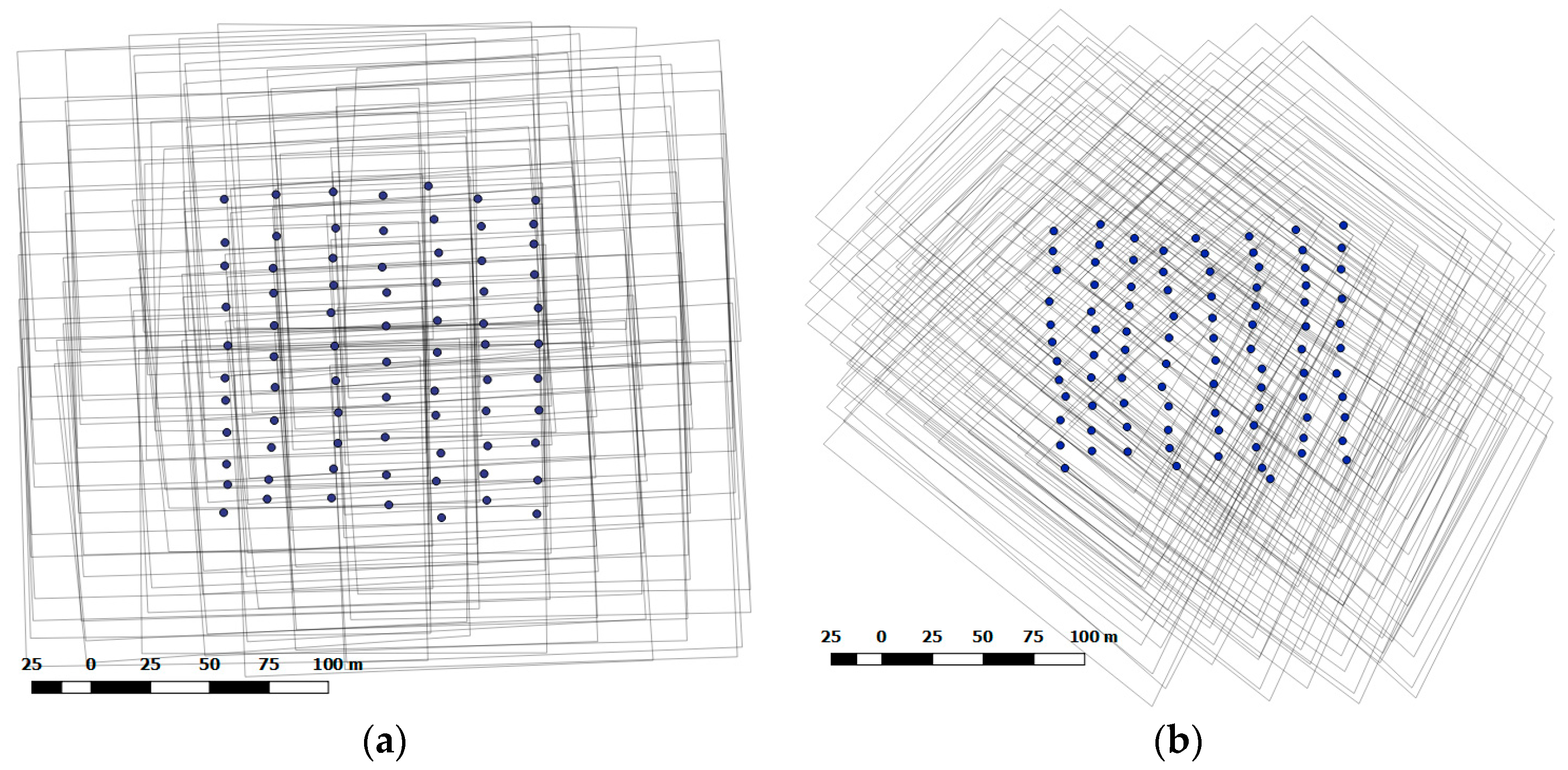
Important factors for the consideration of bundle-block adjustment accuracy include the number of GCPs needed for image georeferencing, their distribution, and camera self-calibration calculations. Agüera-Vega [31] and Goldstein [32] showed that optimal results for UAS image bundle-block adjustment and SfM can be reached with 10–15 signalised GCPs. In our case, the GCP measurements were performed after the image data acquisition, so we were restricted to measuring well identified man-made (poles, concrete slab corners) and natural (tree stumps) objects. Due to the limited number of such GCPs across the study area, the height (Z) GCPs were added to preserve the block homogenous accuracy. As vertical accuracy of the bundle-block adjustment is extremely influential on tree heights measurements, we suggest measuring additional non-signalised or even signalised height (Z) GCPs across the study area, based on a regular locational pattern. In this study, the Photomod package produced better results related to the enhanced vertical accuracy of the bundle-block adjustment; these were attributable to the stereo mode for GCP manual measurements, which is not available in PhotoScan.

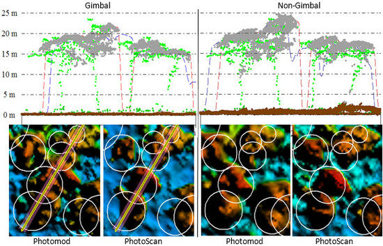
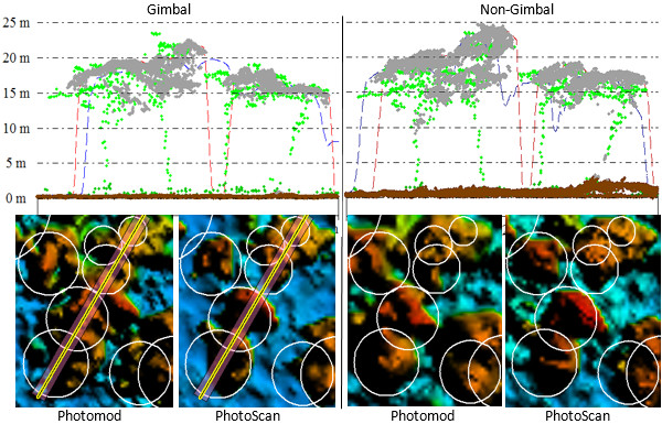
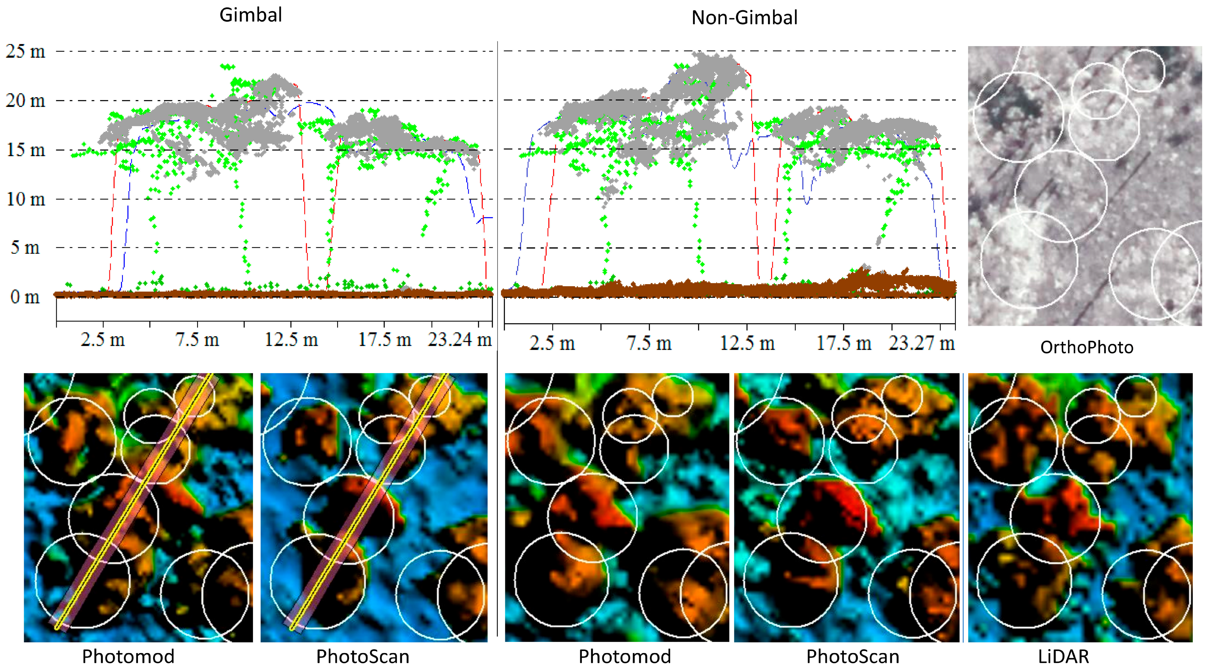
The accurate representation of the terrain is crucial for characterising the 3D structure of vegetation, which is necessary for CHM calculations [15]. The current study found that the Eucalyptus spp. savanna vegetation structure is sufficiently transparent for accurate terrain reconstruction by SfM matching techniques. Based on our results, ~50% of all 3D point cloud extracted points related to the ground surface, which negates the need to use an external digital terrain model for CHM generation (Figure 6). On the other hand, crown transparency had a direct impact on tree detection rates using SfM matching. These findings suggest that the optimal image data acquisition time is between the end of the wet and start of the dry seasons, when canopy cover of Australian tropical savanna is at maximum [33]. Overall, SfM-based ground surfaces provided an accurate and applicable representation of the terrain across the study plot (Table 2). The largest differences in the non-gimbal SfM-based models likely originated from the poor reconstructed image geometry during image block relative orientation (tie point matching) and 3D point cloud SfM calculations (high noise; Figure 6).

The spatial resolution of the CHM greatly impacts the detectability of small trees <10 m (omission error), whilst simultaneously impacting the local maxima detection of tall tree crowns (commission error). We found that small, understorey, and intermediate trees could not be reliably identified with the local maxima approach at all resolutions, where the detection rate was 35% at 0.3–0.4 m CHM resolution, and reduced to 25% at 1 m CHM resolution. 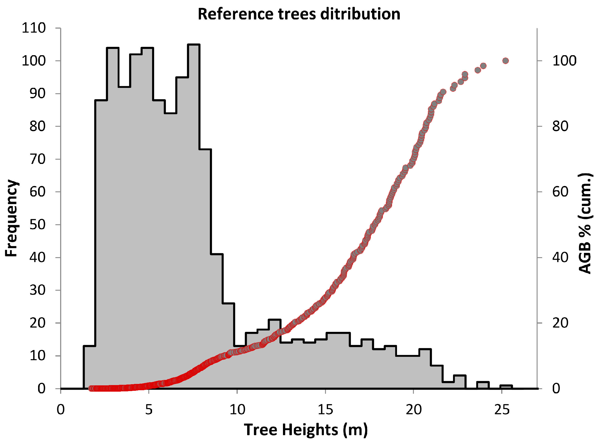Similarly, depending on the ITD approach, many other LiDAR studies [34,35,36,37] demonstrate similarly low detection rates of small trees (<40%), describing poor representativeness in point clouds due to overstory obscuration. However, in our study, the omission error for trees <10 m, had a minor influence on the final biomass estimates, since all of the small trees account for only 13% of total AGB.

The occurrence of false tree peaks (H > 10 m) added further challenges. The ~40% commission error is related to multi-local maxima in corresponding tree crowns, while the remaining proportion represent falsely detected trees. We found that using the 0.3-m CHM significantly increased (by ~100%) the number of extra local maxima in corresponding tree crowns. In turn, this led to greater commission errors and substantial AGB overestimation. The detection of dominant and co-dominant trees remained stable for the 0.5 and 1 m CHMs resolutions, providing a reliable tree detection rate (65–70%) for tropical Eucalyptus spp. savanna (Table 3).

Despite all models (Table 4 and Table 5) showing similar tree detection rates, our findings demonstrated slightly better results related to models based on the PhotoScan 3D point cloud, especially with watershed segmentation. This variance could be attributed to the different matching algorithms that were used in the two software packages. Although all of the SfM-based models showed generally adequate tree detection rates, LiDAR-based measurements were better by 17% for all of the trees, and by 9% for dominant and co-dominant trees. Comparison of the LiDAR and SfM point cloud vertical profiles (Figure 6) show that SfM did not capture the foliage distribution of the midstory and understory canopy layers. At the same time, the SfM point cloud provided a greater point density than the LiDAR data, depending only on image resolution, and used matching algorithms. It is likely that the discrepancy in detection rates between the LiDAR and SfM data could be partly ameliorated by using a camera with a larger sensor and oblique imagery, which is an important consideration for future research.

Another issue related to tree detection accuracy was the significant effect of the local maxima search window size relative to the tree crown size. Therefore, filter dimensions require careful selection [26,38]. As a result, individual tree detection accuracy can be improved through clarification of height–crown diameter relationships before each project when undertaking the canopy maxima approach. Therefore, it may be the case that watershed segmentation can be used as a key tree detection approach, as it does not need the height–crown diameter relationship calculation. To minimise tree detection commission errors, the watershed segmentation needs a definition of the threshold value for segments to join. Another advantage of watershed segmentation use over a local maxima approach is that it provides additional tree attributes, such as crown delineation and canopy area data. Similarly, the watershed segmentation approach cannot correctly extract tree segment areas, due to considerable variation in crown diameter and the crown transparency of dominant and co-dominant Eucalypt trees. Thus, the crown area segments extracted by the watershed segmentation cannot improve the AGB estimation of Eucalypt trees in Australian tropical savannas.

4.2. The Effect of Camera Calibration Precision on the Accuracy of Tree Height and Biomass Estimation

In this study, the accuracy of the CHM had a direct effect on final AGB estimation, given indirect allometry based only on tree height. Under/overestimation of tree heights (Table 6) led to corresponding variation in plot AGB estimation, from −11% to +15% for trees (H > 10 m), depending on the model (except in the case of the non-gimbal PhotoScan model). The Photomod gimbal-based CHMs tended to underestimate tree height (~−25 cm mean), while the PhotoScan models overestimated (~+10 cm mean). The tree height underestimation in the Photomod models can be partly explained by smoothing filters and the interpolation process applied during the DSM creation from the 3D point cloud. 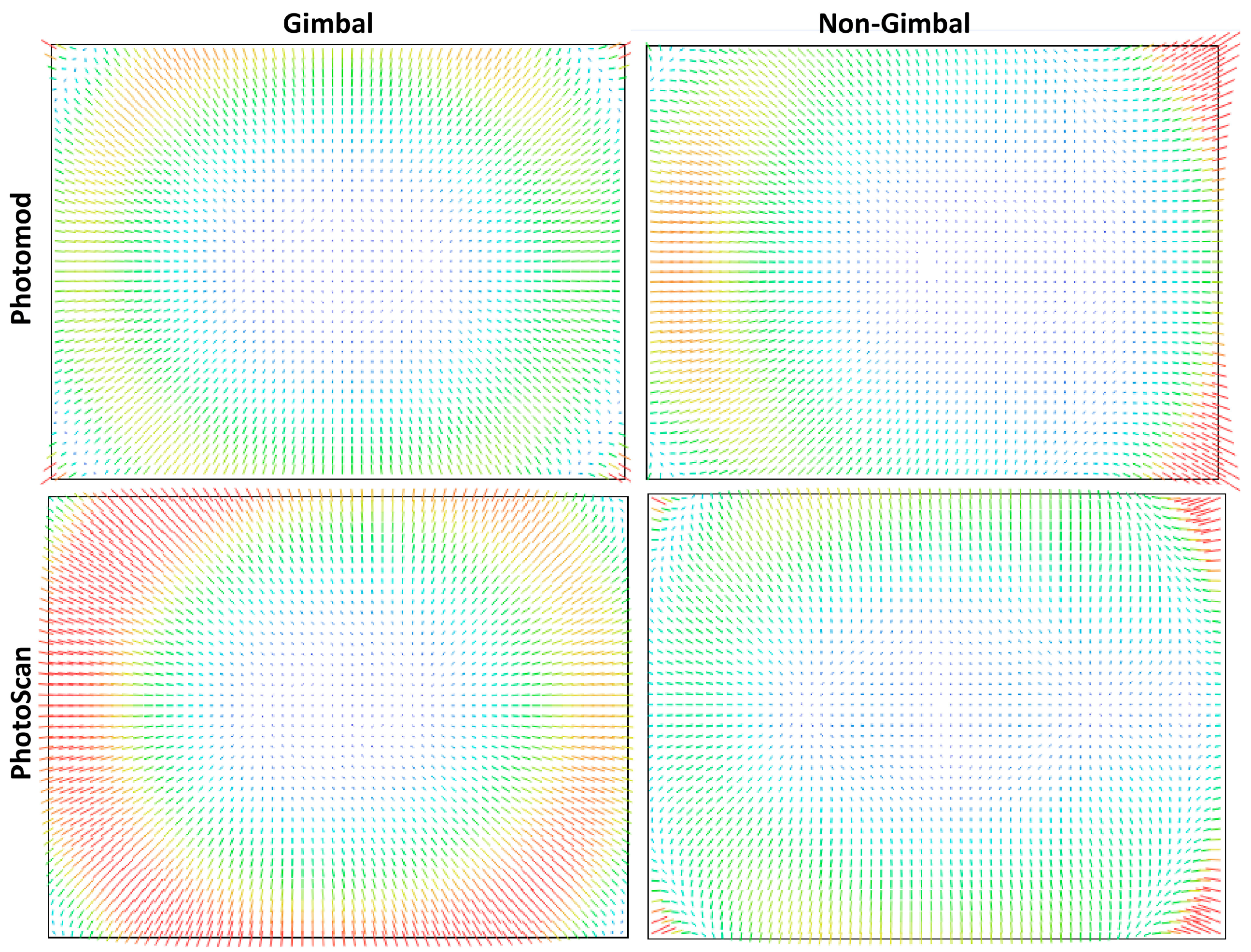As well, the results from Photomod and PhotoScan are likely to be related to volatility and errors in the camera’s self-calibration process during the independent block-bundle adjustments (Figure 7), which therefore affected the vertical accuracy of the extracted digital surface model [39].

The differences in the self-calibration results may be explained, firstly, by all of the GCPs being located on flat terrain (<0.5 m height range), which is disadvantageous in terms of accuracy and correlation between camera parameters; it is a non-optimal approach to producing metrically corrected and scene-independent calibration [40]. Based on James and Robson [39], another possible explanation for this discrepancy is that the self-calibrating bundle adjustment of non-metric cameras may not be able to derive lens radial distortion accurately, resulting in a systematic vertical error possibly remaining, even with sufficient numbers of GCPs. We anticipate that a camera with a larger sensor and detector pixel size could provide better accuracy in tree height estimation due to its more stable internal sensor geometry and better radiometry.

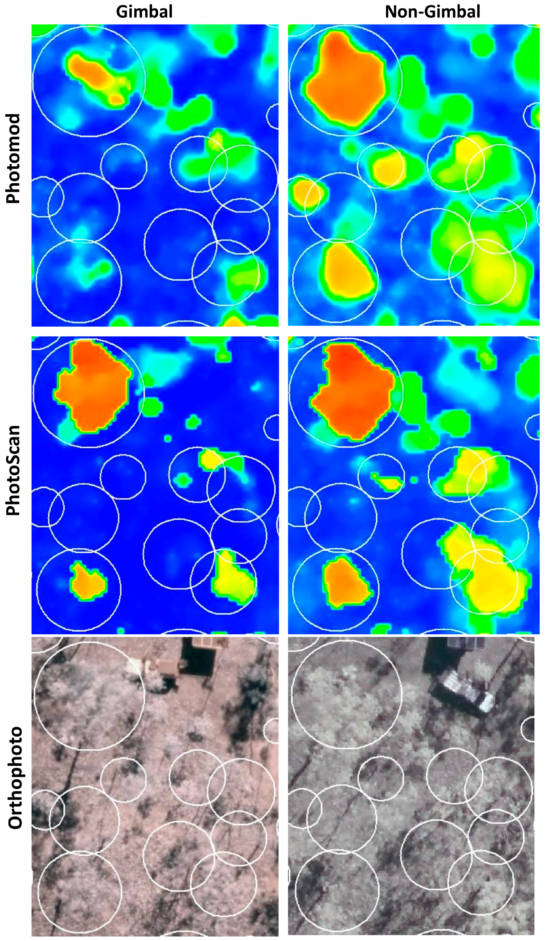
The Photomod-based model of the non-gimbal flight provided slightly better results in comparison with the gimbal flight, especially in the case of several tall tree detections (Figure 8). These results are likely related to noticeable changes of camera orientation angles, and the fact that the camera was not angled at nadir during the non-gimbal flight. Besides self-calibration issues, the tree detection omission and commission errors do not compensate for each other, which obviously leads to systematic under/overestimation of AGB in each corresponding model.

4.3. Aspects and Limitations of Data Acquisition by GoPro HERO4 Camera

The main limitation of the GoPro camera is that the very small sensor (1.55 µm detector pixel size), in combination with a small lens aperture, has low sensitivity to light (low signal to noise ratio and low dynamic range). Additionally, the operations of the camera are limited by the availability of automatic shooting and continuous data acquisition modes (1 s in our case) only. As a result, to provide a sufficient shutter speed (<1/1000 s) for image acquisition, the camera must be operated in sunny conditions with a sun angle >50°. Hence, we do not recommend using the acquired GoPro imagery without basic radiometry pre-processing (contrast, sharpness, etc.).

Direct georeferencing, based only on on-board GoPro GPS data, cannot be used for accurate forestry applications due to the low accuracy of the mobile GPS (5–20 m absolute error, in our case). The GCPs must be measured for indirect image georeferencing and camera self-calibration. This study, and our experience in UAS data processing, has demonstrated that on-board GPS precision is not a major factor defining successful UAS imagery processing results. The ability to deliver radiometrically corrected and undistorted images with high overlap and stable camera orientation angles is more important, which is in agreement with Bosak [41]. This can be achieved by camera platform-stabilising (gimbal use) during data acquisition. Despite the non-gimbal acquisition reducing the cost and weight of the equipment and sometimes providing better results in tree detection (Figure 8), we recommend using a gimbal for accurate UAS mapping. The gimbal can help prevent unexpected problems related to image block relative orientation (tie point matching) and 3D point cloud matching (high noise, which has impact on point classification accuracy (Table 2; Figure 6)). In most cases, the problems we’ve mentioned cannot be solved by an inexperienced user, and require highly skilled photogrammetric ability and experience and comprehensive software tools (stereo mode, pair-wise error deep analysis etc.). Taking all these factors together, we conclude that a GoPro camera with gimbal can be used for the AGB estimation of the dominant and co-dominant trees in Australian tropical savannas, with a plot accuracy ±15% (without counting both small and understory tress). Furthermore, the limitation of this study related to fact that presented individual tree detection results can be applied only in local areas with similar Eucalyptus spp. vegetation.

5. Conclusions

The main aim of this study was to evaluate the efficiency of consumer light-weight and low-cost UAS imagery (<$2000) for estimating tree structural parameters and quantifying biomass in Australian tropical savannas based on well-known canopy maxima and watershed segmentation tree detection algorithms. We found that the canopy maxima and watershed segmentation routines could achieve similar tree detection rates (~70%) for dominant and co-dominant trees, but low detection rates (<35%) for small trees due to poor representativeness in the point clouds and overstory obscuration. The GoPro camera, with a gimbal setup and a sufficient number of GCPs, can be used for an acceptable (±1.2 m) height estimation of dominant and co-dominant trees. We conclude that this low-cost UAS option currently cannot be used for reliable AGB estimation due to unstable sensor internal geometry, which affected the vertical accuracy of extracted CHMs. Although LiDAR data provides higher tree detection rates and more accurate estimates of tree heights, image matching was found to be an adequate low-cost alternative for the detection of dominant and co-dominant tree stands in Australian tropical savannas.

References

1. Trumbore, S.; Brando, P.; Hartmann, H. Forest health and global change. Science 2015, 349, 814–818. [Google Scholar] [CrossRef] [PubMed]
2. Maltamo, M.; Næsset, E.; Vauhkonen, J. Forestry Applications of Airborne Laser Scanning Concepts and Case Studies; Springer: Berlin/Heidelberg, Germany, 2014; Volume 27. [Google Scholar]
3. Lefsky, M.A.; Cohen, W.B.; Harding, D.J.; Parker, G.G.; Acker, S.A.; Gower, S.T. Lidar remote sensing of above-ground biomass in three biomes. Glob. Ecol. Biogeogr. 2002, 11, 393–399. [Google Scholar] [CrossRef]
4. Asner, G.P.; Mascaro, J. Mapping tropical forest carbon: Calibrating plot estimates to a simple LiDAR metric. Remote Sens. Environ. 2014, 140, 614–624. [Google Scholar] [CrossRef]
5. Goldbergs, G.; Levick, S.R.; Lawes, M.; Edwards, A. Hierarchical integration of individual tree and area-based approaches for savanna biomass uncertainty estimation from airborne LiDAR. Remote Sens. Environ. 2018, 205, 141–150. [Google Scholar] [CrossRef]
6. Colomina, I.; Molina, P. Unmanned aerial systems for photogrammetry and remote sensing: A review. ISPRS J. Photogramm. Remote Sens. 2014, 92, 79–97. [Google Scholar] [CrossRef]
7. Westoby, M.J.; Brasington, J.; Glasser, N.F.; Hambrey, M.J.; Reynolds, J.M. ‘Structure-from-Motion’ photogrammetry: A low-cost, effective tool for geoscience applications. Geomorphology 2012, 179, 300–314. [Google Scholar] [CrossRef] [Green Version]
8. Torresan, C.; Berton, A.; Carotenuto, F.; Di Gennaro, S.F.; Gioli, B.; Matese, A.; Miglietta, F.; Vagnoli, C.; Zaldei, A.; Wallace, L. Forestry applications of UAVs in Europe: A review. Int. J. Remote Sens. 2017, 38, 2427–2447. [Google Scholar] [CrossRef]
9. Tang, L.; Shao, G. Drone remote sensing for forestry research and practices. J. For. Res. 2015, 26, 791–797. [Google Scholar] [CrossRef]
10. Paneque-Gálvez, J.; McCall, M.; Napoletano, B.; Wich, S.; Koh, L. Small Drones for Community-Based Forest Monitoring: An Assessment of Their Feasibility and Potential in Tropical Areas. Forests 2014, 5, 1481. [Google Scholar] [CrossRef]
11. Beringer, J.; Hutley, L.B.; Abramson, D.; Arndt, S.K.; Briggs, P.; Bristow, M.; Canadell, J.G.; Cernusak, L.A.; Eamus, D.; Edwards, A.C.; et al. Fire in Australian savannas: From leaf to landscape. Glob. Chang. Biol. 2015, 21, 62–81. [Google Scholar] [CrossRef] [PubMed] [Green Version]
12. Williams, R.; Hutley, L.B.; Cook, G.D.; Russell-Smith, J.; Edwards, A.; Chen, X. Assessing the carbon sequestration potential of mesic savannas in the Northern Territory, Australia: Approaches, uncertainties and potential impacts of fire. Funct. Plant Biol. 2004, 31, 415–422. [Google Scholar] [CrossRef]
13. Russell-Smith, J.; Murphy, B.P.; Meyer, C.P.; Cooka, G.D.; Maier, S.; Edwards, A.C.; Schatz, J.; Brocklehurst, P. Improving estimates of savanna burning emissions for greenhouse accounting in northern Australia: Limitations, challenges, applications. Int. J. Wildland Fire 2009, 18, 1–18. [Google Scholar] [CrossRef]
14. Hung, C.; Bryson, M.; Sukkarieh, S. Multi-class predictive template for tree crown detection. ISPRS J. Photogramm. Remote Sens. 2012, 68, 170–183. [Google Scholar] [CrossRef]
15. Wallace, L.; Lucieer, A.; Malenovský, Z.; Turner, D.; Vopěnka, P. Assessment of Forest Structure Using Two UAV Techniques: A Comparison of Airborne Laser Scanning and Structure from Motion (SfM) Point Clouds. Forests 2016, 7, 62. [Google Scholar] [CrossRef]
16. Wallace, L.; Lucieer, A.; Watson, C.; Turner, D. Development of a UAV-LiDAR System with Application to Forest Inventory. Remote Sens. 2012, 4, 1519. [Google Scholar] [CrossRef]
17. Whiteside, T.G.; Bartolo, R.E. Robust and Repeatable Ruleset Development for Hierarchical Object-Based Monitoring of Revegetation Using High Spatial and Temporal Resolution UAS Data. In Proceedings of the GEOBIA 2016: Solutions and Synergies, Enschede, The Netherlands, 14–16 September 2016. [Google Scholar]
18. TERN. Litchfield Savanna SuperSite. Available online: http://www.tern-supersites.net.au/supersites/lfld (accessed on 30 March 2015).
19. Beringer, J.; Hacker, J.; Hutley, L.B.; Leuning, R.; Arndt, S.K.; Amiri, R.; Bannehr, L.; Cernusak, L.A.; Grover, S.; Hensley, C.; et al. SPECIAL—Savanna Patterns of Energy and Carbon Integrated across the Landscape. Bull. Am. Meteorol. Soc. 2011, 92, 1467–1485. [Google Scholar] [CrossRef]
20. O’Grady, A.P.; Chen, X.; Eamus, D.; Hutley, L.B. Composition, leaf area index and standing biomass of eucalypt open forests near Darwin in the Northern Territory, Australia. Aust. J. Bot. 2000, 48, 629–638. [Google Scholar] [CrossRef]
21. Isenburg, M. LAStools—Efficient LiDAR Processing Software (Version 141017, Unlicensed). Available online: https://rapidlasso.com/lastools/ (accessed on 30 May 2015).
22. McGaughey, R.J. FUSION/LDV: Software for LIDAR Data Analysis and Visualization; Version 3.50; US Department of Agriculture, Forest Service, Pacific Northwest Research Station: Seattle, WA, USA, 2015.
23. Hirschmüller, H. Semi-global matching-motivation, developments and applications. In Proceedings of the Photogrammetric Week 11, Stuttgart, Germany, 9–13 September 2011; pp. 173–184. [Google Scholar]
24. Agisoft. PhotoScan Community Forum Topic: Algorithms Used in Photoscan. Available online: http://www.agisoft.com/forum/index.php?topic=89.msg13780;topicseen#msg13780 (accessed on 27 February 2017).
25. Kaartinen, H.; Hyyppä, J.; Yu, X.; Vastaranta, M.; Hyyppä, H.; Kukko, A.; Holopainen, M.; Heipke, C.; Hirschmugl, M.; Morsdorf, F. An international comparison of individual tree detection and extraction using airborne laser scanning. Remote Sens. 2012, 4, 950–974. [Google Scholar] [CrossRef] [Green Version]
26. Popescu, S.C.; Wynne, R.H.; Nelson, R.F. Estimating plot-level tree heights with lidar: Local filtering with a canopy-height based variable window size. Comput. Electron. Agric. 2002, 37, 71–95. [Google Scholar] [CrossRef]
27. Li, W.; Guo, Q.; Jakubowski, M.K.; Kelly, M. A new method for segmenting individual trees from the lidar point cloud. Photogramm. Eng. Remote Sens. 2012, 78, 75–84. [Google Scholar] [CrossRef]
28. Goutte, C.; Gaussier, E. A probabilistic interpretation of precision, recall and F-score, with implication for evaluation. In Proceedings of the 27th European conference on Advances in Information Retrieval Research (ECIR), Santiago de Compostela, Spain, 21–23 March 2005; pp. 345–359. [Google Scholar]
29. Conrad, O.; Bechtel, B.; Bock, M.; Dietrich, H.; Fischer, E.; Gerlitz, L.; Wehberg, J.; Wichmann, V.; Böhner, J. System for Automated Geoscientific Analyses (SAGA) v. 2.1.4. Geosci. Model Dev. 2015, 8, 1991–2007. [Google Scholar] [CrossRef]
30. QGIS. QGIS Geographic Information System. Open Source Geospatial Foundation Project. Available online: http://www.qgis.org (accessed on 30 May 2015).
31. Agüera-Vega, F.; Carvajal-Ramírez, F.; Martínez-Carricondo, P. Assessment of photogrammetric mapping accuracy based on variation ground control points number using unmanned aerial vehicle. Measurement 2017, 98, 221–227. [Google Scholar] [CrossRef]
32. Goldstein, E.B.; Oliver, A.R.; de Vries, E.; Moore, L.J.; Jass, T. Ground control point requirements for structure-from-motion derived topography in low-slope coastal environments. PeerJ PrePrints 2015, 3, e1444v1441. [Google Scholar] [CrossRef]
33. Russell-Smith, J.; Murphy, B.; Edwards, A.; Meyer, C.P. Carbon Accounting and Savanna Fire Management; CSIRO Publishing: Clayton, Australia, 2015. [Google Scholar]
34. Ferraz, A.; Bretar, F.; Jacquemoud, S.; Gonçalves, G.; Pereira, L.; Tomé, M.; Soares, P. 3-D mapping of a multi-layered Mediterranean forest using ALS data. Remote Sens. Environ. 2012, 121, 210–223. [Google Scholar] [CrossRef]
35. Reitberger, J.; Schnörr, C.; Krzystek, P.; Stilla, U. 3D segmentation of single trees exploiting full waveform LIDAR data. ISPRS J. Photogramm. Remote Sens. 2009, 64, 561–574. [Google Scholar] [CrossRef]
36. Duncanson, L.I.; Cook, B.D.; Hurtt, G.C.; Dubayah, R.O. An efficient, multi-layered crown delineation algorithm for mapping individual tree structure across multiple ecosystems. Remote Sens. Environ. 2014, 154, 378–386. [Google Scholar] [CrossRef]
37. Edson, C.; Wing, M.G. Airborne Light Detection and Ranging (LiDAR) for Individual Tree Stem Location, Height, and Biomass Measurements. Remote Sens. 2011, 3, 2494–2528. [Google Scholar] [CrossRef] [Green Version]
38. Turner, R.S. An Airborne Lidar Canopy Segmentation Approach for Estimating Above-Ground Biomass in Coastal Eucalypt Forests. Ph.D. Thesis, University of New South Wales, Sydney, Australia, 2006. [Google Scholar]
39. James, M.R.; Robson, S. Mitigating systematic error in topographic models derived from UAV and ground-based image networks. Earth Surf. Process. Landf. 2014, 39, 1413–1420. [Google Scholar] [CrossRef]
40. Luhmann, T.; Fraser, C.; Maas, H.-G. Sensor modelling and camera calibration for close-range photogrammetry. ISPRS J. Photogramm. Remote Sens. 2016, 115, 37–46. [Google Scholar] [CrossRef]
41. Bosak, K. Secrets of UAV Photomapping. Pteryx: Poland, 2011. Available online: http://www.academia.edu/download/32814759/pteryx-mapping-secrets.pdf (accessed on 30 September 2014).
Figure 1. The height class and cumulative aboveground biomass (AGB) (red line) distribution of reference trees (n = 1277) in the 2.2 ha study area.
Remotesensing 10 00161 g001
Figure 2. The 2.2 ha study area: (a) with ground control points (GCPs) locations (∆—full GCP (XYZ), O—height GCP (Z)); (b) dominated by Eucalyptus spp.; (c) in the north Australian tropical savanna (in green).
Remotesensing 10 00161 g002
Figure 3. Workflow outline for this case. The two unmanned aerial systems (UAS) imagery sets with and without gimbal setup, and light detection and ranging (LiDAR) reference data were used to perform individual tree detection and AGB estimation. The software used are shown in blue boxes.
Remotesensing 10 00161 g003
Figure 4. The block schemes (imagery footprints and projection centers) of two unmanned aerial systems (UAS) flights based on block adjustment results (Photomod) (a) with gimbal, and (b) without gimbal.
Remotesensing 10 00161 g004
Figure 5. Study area subset (35 × 42 m) of Photomod processed raster canopy height models (CHMs) with different ground sample distance (GSD) resolutions, and applied a 3 × 3 smoothing kernel filter. (a) Original 10-cm GSD; (b) 30 cm; (c) 40 cm; (d) 1 m and (e) LiDAR 50-cm CHM. White circles represent the crowns of reference trees (height > 10 m).
Remotesensing 10 00161 g005
Figure 6. Horizontal transect (1.6 m wide) of study area subset. Reference LiDAR three-dimensional (3D) point cloud (green dots), PhotoScan extracted point cloud (grey dots—vegetation; brown dots—classified terrain), Photomod digital surface model (DSM) (blue line), PhotoScan DSM (red line), and their corresponding 40 cm raster DSMs used for local maxima and watershed segmentation.
Remotesensing 10 00161 g006
Figure 7. GoPro camera lens distortion plots based on camera self-calibration results in Photomod and PhotoScan. The estimated camera distortions are presented at the same scale (×161) across all of the figures.
Remotesensing 10 00161 g007
Figure 8. Study area subsets (28 × 24 m) demonstrating the better results of the non-gimbal over the gimbal-derived raster CHMs. CHM resolution is 40-cm GSD. White circles represent the crowns of reference trees (height > 10 m).
Remotesensing 10 00161 g008