Crustal Deformation Prior to the 2017 Jiuzhaigou, Northeastern Tibetan Plateau (China), Ms 7.0 Earthquake Derived from GPS Observations


1
College of Surveying and Geo-informatics, Tongji University, Shanghai 200092, China
2
Institute of Earthquake Forecasting, China Earthquake Administration, Beijing 100036, China
*
Author to whom correspondence should be addressed.
Remote Sens. 2018, 10(12), 2028; https://doi.org/10.3390/rs10122028
Submission received: 4 November 2018
/
Revised: 29 November 2018
/
Accepted: 11 December 2018
/
Published: 13 December 2018
(This article belongs to the Special Issue Remote Sensing of Tectonic Deformation)
Abstract
:The 2017 Jiuzhaigou Ms 7.0 earthquake occurred on the northeastern margin of the Tibetan Plateau, with no noticeable rupture surface recognized. We characterized the pre-seismic deformation of the earthquake from GPS (Global Positioning System) data at eight continuous and 73 campaign sites acquired over the 2009–2017 period. With respect to the Eurasian plate, the velocity field showed a noticeable decrease, from west of the epicenter of the Jiuzhaigou earthquake to the western edge of the Longmenshan fault, in the southeast direction. The total northwest west–southeast east shortening rate in the vicinity of the epicentral area was in the range of 1.5 mm/y to 3.1 mm/y. With a GPS velocity transect across the Huya fault (HYF), where the epicenter was located, we estimated the activity of the HYF, showing a dominant left-lateral slip rate of 3.3 ± 0.2 mm/y. We calculated strain rates using a spherical wavelet-based multiscale approach that solved for the surface GPS velocity according to multiscale wavelet basis functions while accounting for spatially variable spacing of observations. Multiscale components of the two-dimensional strain rate tensor showed a complex crustal deformation pattern. Our estimates of strain rate components at the scale of seven and eight revealed extensional strain rate on the northern extension of the HYF. The Jiuzhaigou earthquake occurred at the buffer zone between extensional and compressional deformation, and with significant maximum shear rates being 100–140 nanostrain/y. In addition, a maximum shear strain rate of 60–120 nanostrain/y appeared around the epicenter of the 2013 Ms 6.6 Minxian–Zhangxian earthquake. These findings imply that inherent multiscale strain rates could be separated to identify strain accumulation related to medium- and large-sized earthquakes.

1. Introduction
The ongoing collision between the Indian and Eurasian plates has caused the eastward extrusion of the Tibetan Plateau and the uplift of Tibet [1,2]. Over the past decades, multiple models were proposed to interpret the tectonic evolution of the Tibetan Plateau. Previous studies claimed that the uplift of Eastern Tibetan Plateau is due to the thickening of brittle crust [3,4] related to thrust fault rooted in the lithosphere with large amounts of slip. However, some researchers argued that a lower crustal flow (channel flow) [5,6], in which low-viscosity material in the lower crust flows outward from the interior of the Plateau and inflates the crust in Eastern Tibet, is responsible for the low-rate east–west shortening across the mountains and within the Sichuan Basin. In both models, Tibet was regarded as moving eastward with respect to the Sichuan Basin across the northeastern borderland of the Bayan Har block, with strain accommodated predominantly by the Longriba fault (LRF), Minjiang fault (MJF), Huya fault (HYF), and other secondary faults in the region [7,8].
The northeastern borderland of the Bayan Har block undergoes remarkable crustal deformation due to the uplift, eastward extrusion, and southeastern escape of the Tibetan Plateau. The regions are bounded by the left-lateral strike-slip East Kunlun fault (EKF) zone at its northern boundary, the left-lateral strike-slip Yushu–Xianshuihe fault (YXF) system at its southern boundary. Its eastern boundary zone is composed of the Longmenshan fault (LMF) zone and several secondary faults at its northwestern extension (Figure 1). The topographic margin of the Tibetan Plateau along the LMF is one of most remarkable continental escarpments on Earth: the elevation rises from ~500 m in the Sichuan Basin to peaks exceeding 6500 m over a horizontal distance of ~50 km [9].
On the evening of (19:46.4, local time) of 8 August 2017, an Ms 7.0 earthquake struck Jiuzhaigou area, Sichuan Province. The earthquake epicenter was located at 103.82°E, 33.20°N, on the northern extension of the HYF, with a focal depth being ~20 km, as registered by the China Earthquake Networks Center (CENC). The devastating earthquake destroyed 73,671 houses to different degrees, and caused heavy damage to the Jiuzhaigou scenic zone, and the UNESCO (United Nations Educational, Scientific, and Cultural Organization)-listed world natural heritage site had to be closed for months. The casualty toll as of 14 August 2017 was 25 dead, 11,305 injured, and six missing [10]. In total, 6838 aftershocks were recorded as of 30 October 2017, with two events being between Ms 4.0–4.9, and one maximum aftershock being Ms 4.8 [11].
The GPS (Global Positioning System) measurements had been conducted in the eastern Bayan Har tectonic block by several institutions prior to the Jiuzhaigou earthquake. Previous studies showed the present-day crustal motion in this region was predominantly southeastward extrusion of the Eastern Tibetan Plateau with respect to the stable Sichuan Basin, part of the South China block (Figure 1). However, several issues remain regarding the crustal deformation regime of this region. What was the strain pattern prior to the recent Ms 7.0 Jiuzhaigou earthquake? Is there any relationship between spatial strain buildup and seismic activities in this region? In this study, we explored the pre-seismic strain based on the GPS observations spanning from 2009 to 2017 and employed a multiscale spherical wavelet approach to calculate strain rate fields, as well as analyzed the correlation between crustal strain and seismicity.
2. Tectonic Setting
The northeastern margin zone of the Bayan Har block exhibits a complex tectonic pattern, with small-scale terranes sliced and bounded by multiple faults [8,12]. The EKF is segmented into an array of the Guanggaishan–Dieshan (GDF), Tazang (TZF), MJF, HYF, and LRF in its eastern part [13]. The LRF, MJF, and the HYF are all active during the Holocene [8]. The NS (north–south)-striking MJF and HYF bound the Minshan Uplift Zone at its western and eastern margins, respectively. Both the faults dip to the west [12].
Geomorphologic studies identify a left-lateral slip rate of ~1 mm/y and a vertical slip rate of ~1 mm/y along the MJF [14]. The crustal shortening is ~0.8 mm/y and >0.3 mm/y in near EW (east–west) direction across the LRF and MJF, respectively [8]. Crustal shortening is around 0.5–0.7 mm/y across the HYF in the near EW direction [14]. The NE (northeast)-striking Wenxian fault (WXF) is also active during late Quaternary, with a shortening rate in the near NS direction being about 1.1 ± 0.1 mm/y [15]. Ms > 4.5 earthquakes since 1976 on the eastern margin of the Bayan Har block show a diffuse spatial distribution (Figure 1). The HYF was ruptured by the 1976 Songpan earthquake sequence, which was composed of two Ms 7.2 and one Ms 6.7 events. The northern segment of the HYF was ruptured during the 1973 Ms 6.5 Huanglong and 2017 Ms 7.0 Jiuzhaigou earthquakes with similar sinistral strike-slip focal mechanisms. The MJF was ruptured by the 1933 Ms 7.5 Diexi, 1938 Ms 6, and 1960 Ms 6.8 earthquakes [16]. Moreover, the Lintan–Dangchang fault (LDF) was ruptured by the recent 2013 Minxian–Zhangxian Ms 6.6 earthquake [16].
The 2017 Jiuzhaigou earthquake occurred on the northern extension of the HYF, where three active faults intersect, that is, the blind northern extensional segment of the HYF, MJF, and TZF [15]. The epicentral zone was recognized as high seismic risk prior to the Jiuzhaigou earthquake, according to an interdisciplinary study [17]. No surface rupture zone was recognized during the field investigation carried out shortly after the Jiuzhaigou event [18]. The major axis azimuth of the seismic intensity ellipse, relocated aftershock distribution, earthquake-triggered bedrock collapse, and landslides in the epicentral zone jointly showed that the faulting of the northern extension of the HYF was causative of the 2017 Jiuzhaigou earthquake [11,15,16].
3. GPS Observations and Data Processing
The GPS observations have been carried out in the northeastern borderland of the Bayan Har block since 1999, when the Crustal Movement Observation Network of China (CMONOC) was initiated, and its successor commenced in 2010, which constitute the backbone of GPS networks in China. In total, 260 continuously operating and 2000 campaign sites of the backbone network in monitoring crustal motion are distributed over the Chinese mainland, of which eight continuous and 59 campaign sites are distributed within the study area (Figure 1). Moreover, we deployed 14 GPS campaign sites throughout the northeastern margin of the Tibetan Plateau with the financial support of the project of the 2008 Wenchuan Ms 8.0 Earthquake and Regional Dynamics (WERD, 973 project).
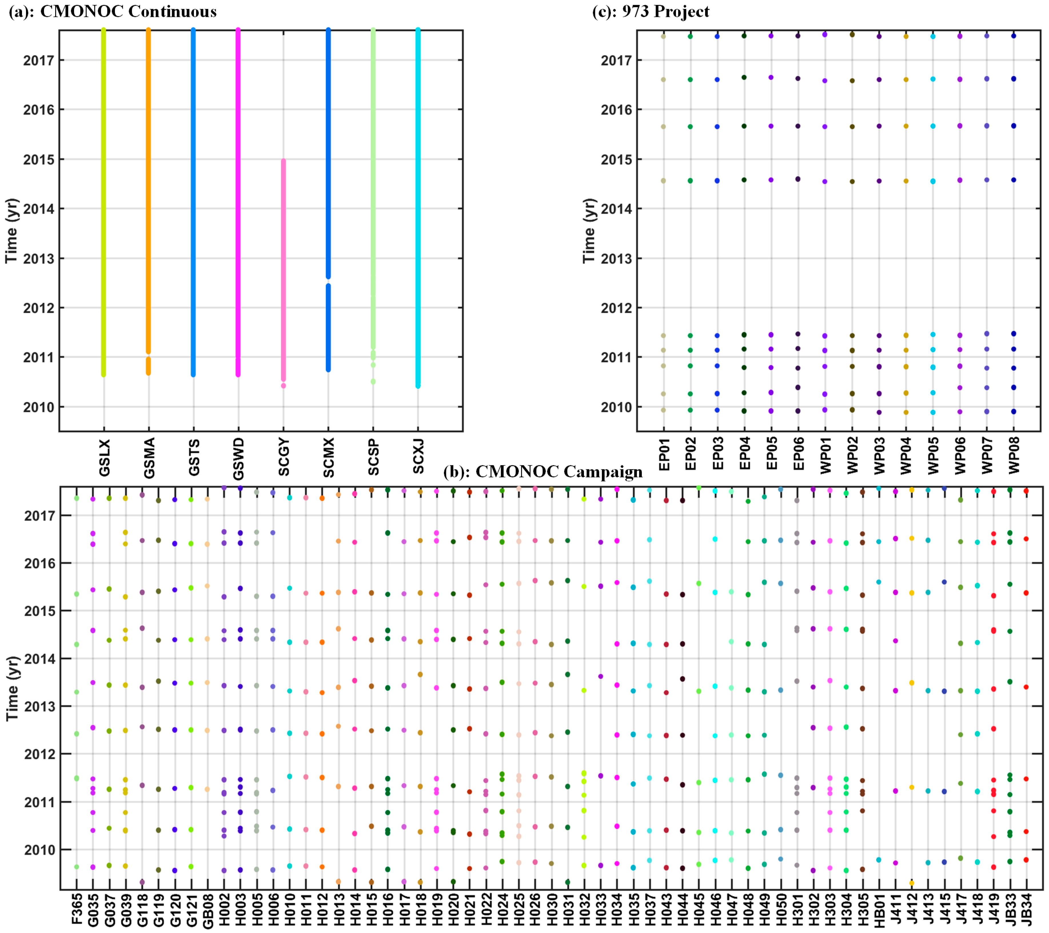
In Figure 2, we present the time occupation history of involved GPS sites. The eight CMONOC continuous sites started operating in late 2010, with one site halted at the end of 2014 and data span for other seven sites being about seven years (Figure 2a). The 59 CMONOC campaign sites are regularly biennially observed, while almost all sites have intensive observations, extending the temporal resolution of observations to be annual or biannual (Figure 2b). The 14 campaign sites from the 973 Project were activated in late 2009, biannually observed in both 2010 and 2011, annually observed from 2014 to 2017, and lack of observations between 2012 and 2014, with nine campaigns in total (Figure 2c). Each site is consecutively observed for three days in each occupation period.
The GAMIT/GLOBK (Global navigation satellite system At Massachusetts Institute of Technology/Global Kalman filter) 10.6 software packages [19] were employed to resolve daily position solutions during the period of 2009–2017. For daily processing of GPS observations, we included all sites (continuous and campaign) from both CMONOC and WERD networks, as well as 127 globally distributed IGS (International Global navigation satellite system Service) sites [20], in constructing the daily network configuration and divided it into several subnetworks with each comprising less than 40 sites. During the resolving of loosely constrained solutions on GAMIT, the sampling frequency and the elevation cut-off angle of GPS observations was set to 30 s and 10°, respectively. The ionosphere-free combination of double-differenced phase observations was formed to eliminate the first-order ionosphere delay effects, and the second-order ionosphere effects [21] were modified by models reported by Petrie et al. [22]. The VMF1 (Vienna Mapping Function type-1) [23] was used to model the dry part of the troposphere delay effects, with atmosphere pressure and temperature parameters collected from station-wise meteorological files and GPT2 (Global Pressure and Temperature version 2) grid files [24]. The IGS14 absolute phase center model was applied to correct the variation of phase center for both satellites and receivers [25]. The FES2004 (Finite Element Solution 2004) tidal model was employed to account for ocean tide corrections [26,27]. Satellite orbits and earth orientation parameters (EOPs) were extracted from IGS ephemeris files. Other classical parameters and models were all referred to the newly updated results from MIT (Massachusetts Institute of Technology, http://www-gpsg.mit.edu). Finally, station position parameters, together with satellite orbits and EOPs, as well as related variance and covariance matrices, were simultaneously estimated as unknowns in the loosely constrained daily solution. During the position estimation stage on GLOBK, loosely constrained solutions were treated as quasi-observations, and minimal constraints were applied to align daily solutions to the International Terrestrial Reference Frame 2014 (ITRF2014) [28] through the six-parameters similarity transformation of 127 evenly distributed sites in globe. With the daily estimation of position solutions on GAMIT/GLOBK, we obtained eight continuous and 73 campaign position time-series in the study area (Figure S1).
4. GPS Velocity Field
For the velocity estimation of continuous GPS sites, each component of the position time-series was modeled with a constant velocity term, two pairs of annual and semiannual sinusoidal variation terms, and several offset terms [29]. As noise model can efficiently affect the estimation of velocity parameters, especially on their accuracy [30], we employed Hector software [31] to estimate noise characteristics and model terms simultaneously. The results showed that the noise model of continuous position time-series was nearly white plus flicker noise model. For the velocity estimation of campaign GPS sites, due to the limited amount of observations, the function model only contained one velocity term, with the statistic model being constructed by white plus flicker noise model, which is analogous to nearby continuous sites. Through above estimation strategies, we obtained an integral ITRF2014 velocity field, with average root mean squares (RMS) of horizontal velocities being ~0.36 mm/y.
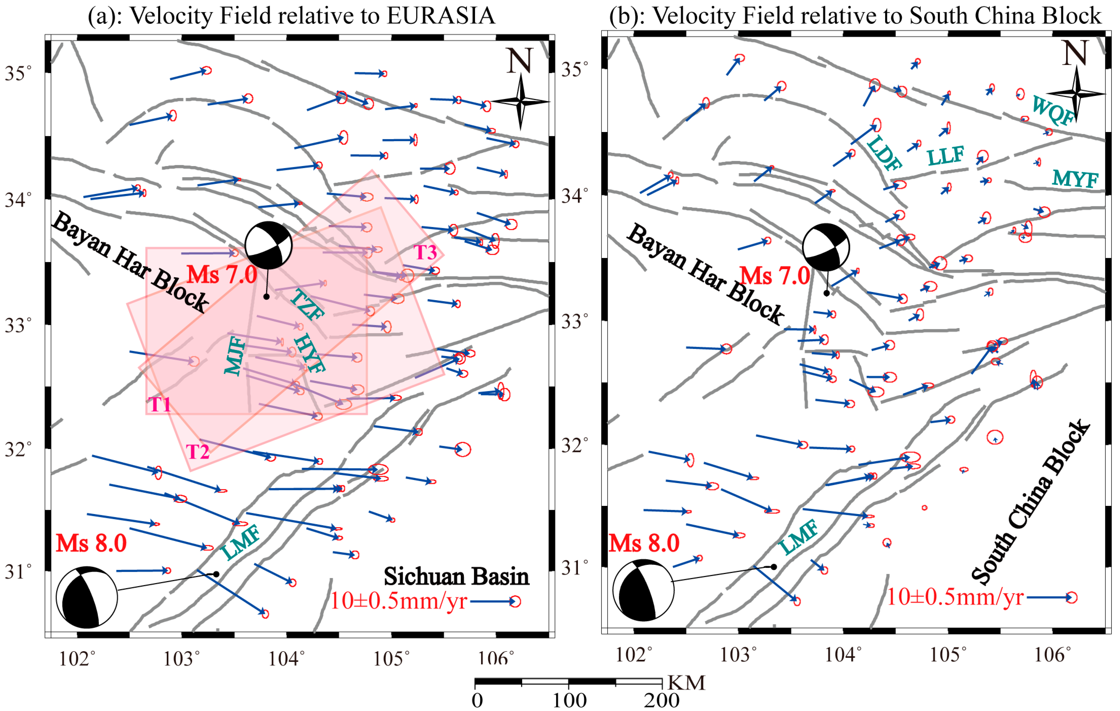
To elaborately depict the pattern of regional crustal deformation, we transformed ITRF2014 velocities into the Eurasia-fixed reference frame [32]. The GPS velocity field with respect to the stable Eurasian plate (Table S1 and Figure 3a) demonstrates that the northeastern margin of the Tibetan Plateau was dominated by southeastward movement. The GPS velocity field gradually decreased from west to east, demonstrating that the eastern extrusion of the Bayan Har block was resisted by the rigid Sichuan Basin and present-day crustal deformation was accommodated by tectonic activities in this region. The velocities are approximately 16.8 ± 0.5 mm/y with orientations at ~110° southwest of the LMF. At the epicentral zone of the Jiuzhaigou earthquake, the GPS velocities are about 11.4 ± 0.4 mm/y, with azimuths being ~105°. The GPS sites move nearly eastward at the zone of 103°E–104.5°E, 34°N–35°N, with an average velocity magnitude being 9.0 ± 0.5 mm/y. At the northeastern part of the study area, GPS velocities are generally 6.8 ± 0.3 mm/y with azimuths being about 110°.
To characterize the pattern of related crustal deformation, we transformed ITRF2014 velocities into a velocity field relative to the South China block. With extra GPS velocities in the Sichuan Basin, we estimated the Euler angular velocity of the South China block with an iterative approach [9]. The angular rotation is 0.3146 ± 0.0583° per million year, with the Euler pole being at (−106.71 ± 1.9484°E, 61.98 ± 1.3864°N). The velocity field with respect to the South China block (Figure 3b) shows that the eastern margin of the Bayan Har block is generally experiencing clockwise rotation. The epicentral zone of the Jiuzhaigou earthquake displays notable velocity decrease from west to east, indicating strain accumulation localized in this zone. No significant deformation was found around the northeastern part of the study zone, where there are four active faults, which are, the West Qinling North fault (WQF), the LDF, Lixian–Luojiapu fault (LLF), and the Mayanhe fault (MYF). Four Ms > 4.5 earthquakes have occurred in this area since 1976, including the 2013 Minxia–Zhangxian Ms 6.6 earthquake, close to the LDF (Figure 1). Around the LMF zone, the velocities are extremely larger than the values from previously published results in Shen et al. [9]. This inconsistency should be attributed to the post-seismic effects of the 2008 Ms 8.0 Wenchuan earthquake, thus contaminating the precise estimation of the velocity field around the epicentral zone of the Wenchuan earthquake.
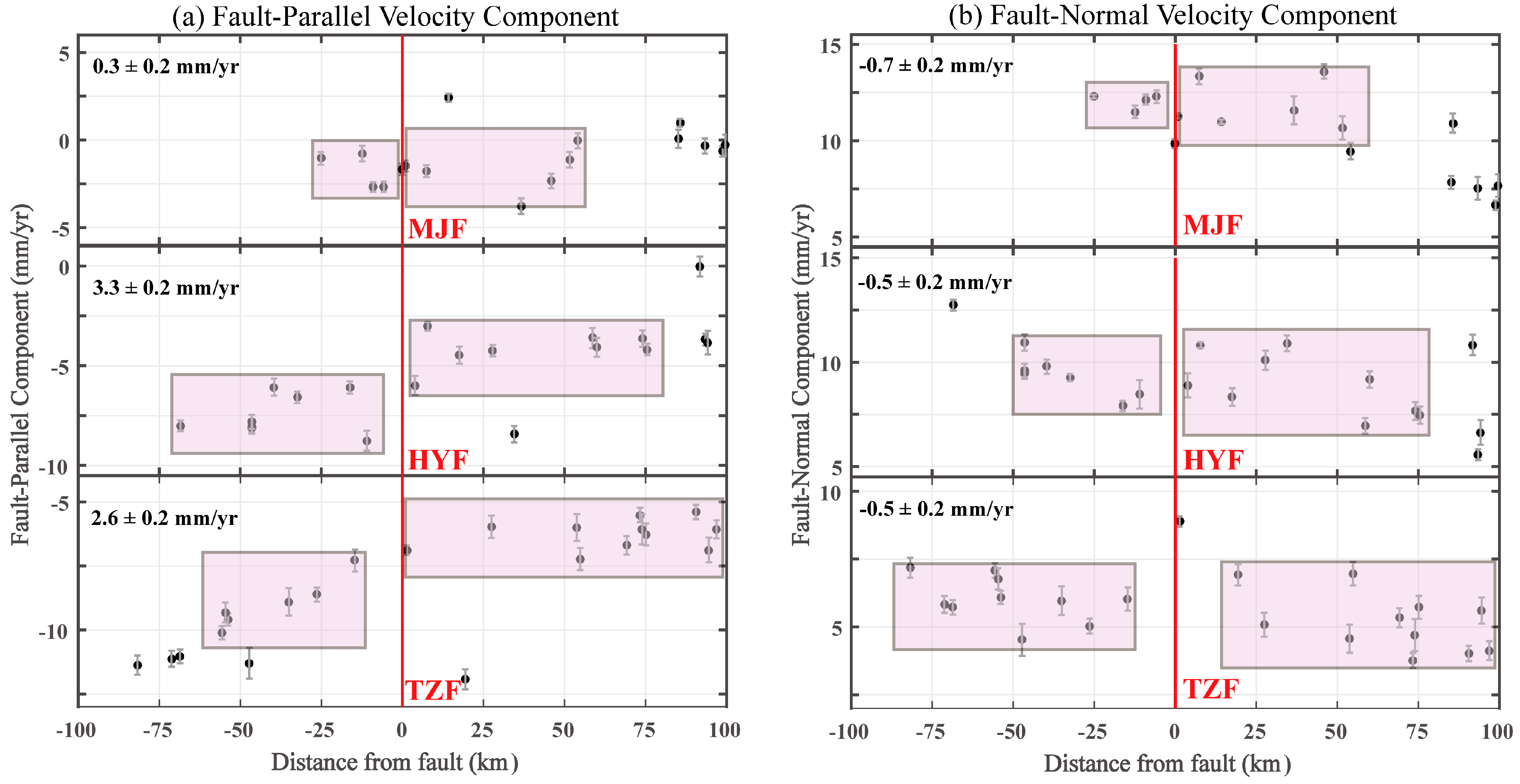
To quantificationally analyze the activities in the epicentral zone (including the MJF, HYF, and TZF) prior to the Jiuzhaigou Ms 7.0 earthquake, we took three GPS velocity profiles to estimate slip rates of these faults. Velocity profiles are shown by the rectangles in Figure 3a. The GPS velocities within the rectangles were decomposed into fault-parallel and fault-normal components, respectively (Figure 4). A noticeable velocity gradient across the HYF was identified from fault-parallel velocity components. However, no significant differential motions were identified for the fault-normal velocity components. We estimated a left-lateral slip rate of 3.3 ± 0.2 mm/y and an insignificant contraction motion of 0.5 ± 0.2 mm/y for the HYF. Moreover, the MJF was found to be less active, with a left-lateral slip rate of 0.3 ± 0.2 mm/y and a compressional motion of 0.7 ± 0.2 mm/y. The results are slightly different from geomorphological studies, which determined that sinistral slips were 1.4 mm/y and 0.37–0.53 mm/y for the HYF and the MJF, respectively [14]. Furthermore, we roughly obtained a 2.6 ± 0.2 mm/y left-lateral-slip motion and a 0.5 ± 0.2 mm/y contraction motion for the eastern part of the TZF with scattered data on its southwestern side. The estimates were nearly consistent with the result of the field investigation, which determined a reverse motion that decreases eastward from ~1.5 mm/y to 0.2–0.3 mm/y (averaged over thousands of years), inferred from a displaced terrace [8].
5. GPS Strain Rate Field
5.1. Methodology
The GPS strain rate can be calculated using various approaches, which can be categorized into two strategies. The first strategy lies on the construction of physical models embedded in elastic half-space or a multi-layered lithosphere of heterogeneous properties with the constraint of GPS velocity field, and the strain rate can be calculated with physical deformation models [33,34,35]. The second strategy exists for calculating 2D (two-dimensional) strain and rotation rates from a GPS velocity field, including Delaunay triangulation [36] and various gridded solutions with multiple mathematical approaches, such as multi-surface function [37], least-square collocation [38], and multiscale spherical wavelet function [39]. In this study, we take the last approach to derive the multiple wavelength strain rate components.
5.1.1. Multiscale Spherical Wavelet Basis Functions
We employ the difference of Gaussian (DOG) wavelet basis function in the decomposition of the velocity field on the sphere [39,40]. The DOG wavelet basis function can be expressed by [39,40]:
where is a constant to adjust the shape of the basis function, and is set to 1.25 (see details in Su et al. [41]) in this study; is the scale expressed as , with being the integer factor and realizing the multiscale purpose; is the angle between the position of the GPS site and the center of the wavelet basis function . The parametric function is expressed as [39]:
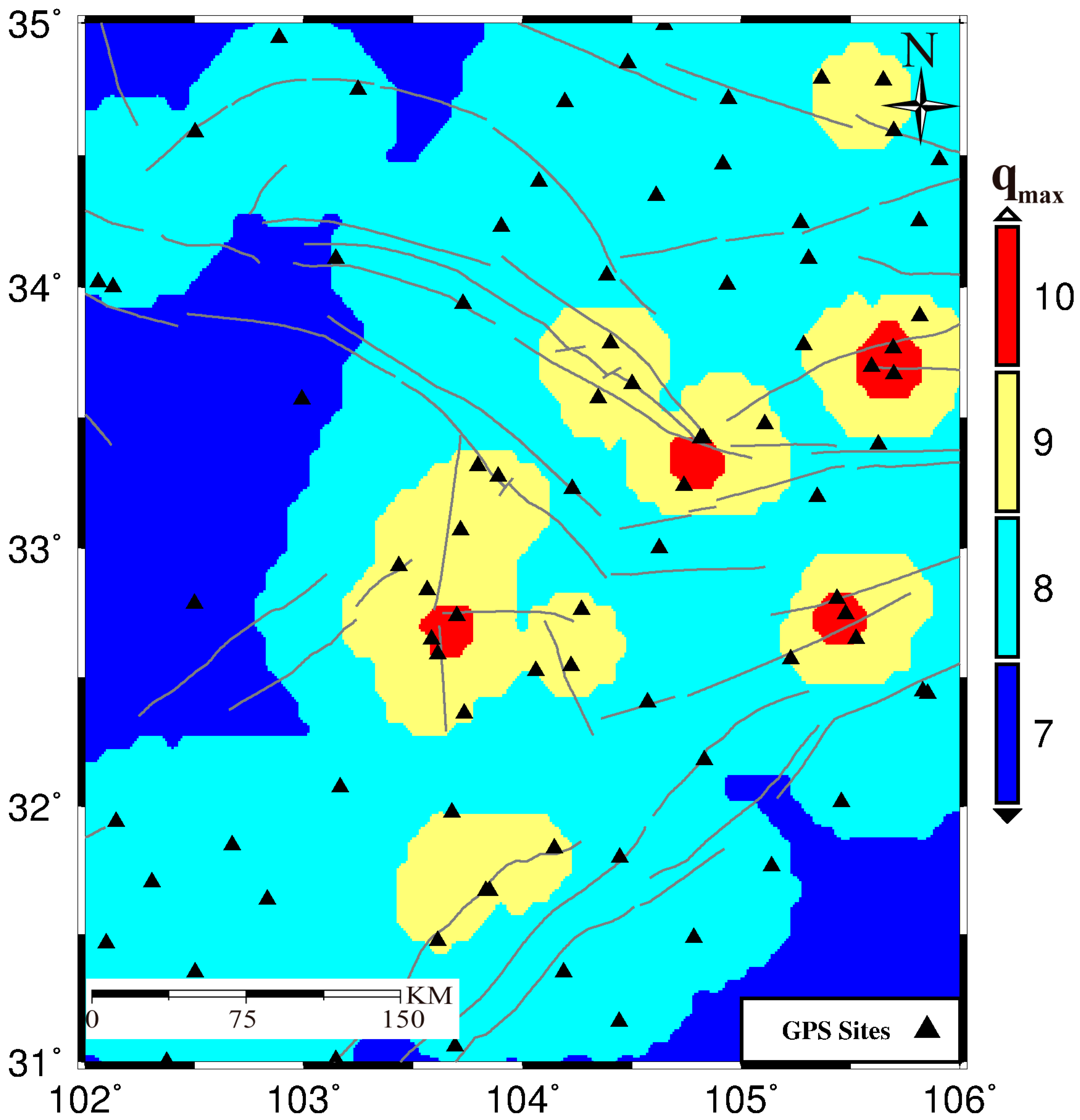
On the selection of the scale factor , the maximum value depends on the spatial density of GPS sites [39,41]. As shown in Figure 5, we present the spatial distribution of the maximum in the study area. Only three small regions can reach , with inter-site distance being less than 6.9 km (see Table 1 in Su et al. [41]), and six discrete regions are with (inter-site distance being 13.8 km). Except for boundary areas, most regions reach with inter-site distance being 27.5 km. To reduce the possibility of overfitting from large scale wavelet functions and stabilizing the estimation problem [39], we restrict to be eight in the following decomposition of the velocity field. As to the minimum value of , it is always constrained by the extent of the study area [39], which is set at in this study.
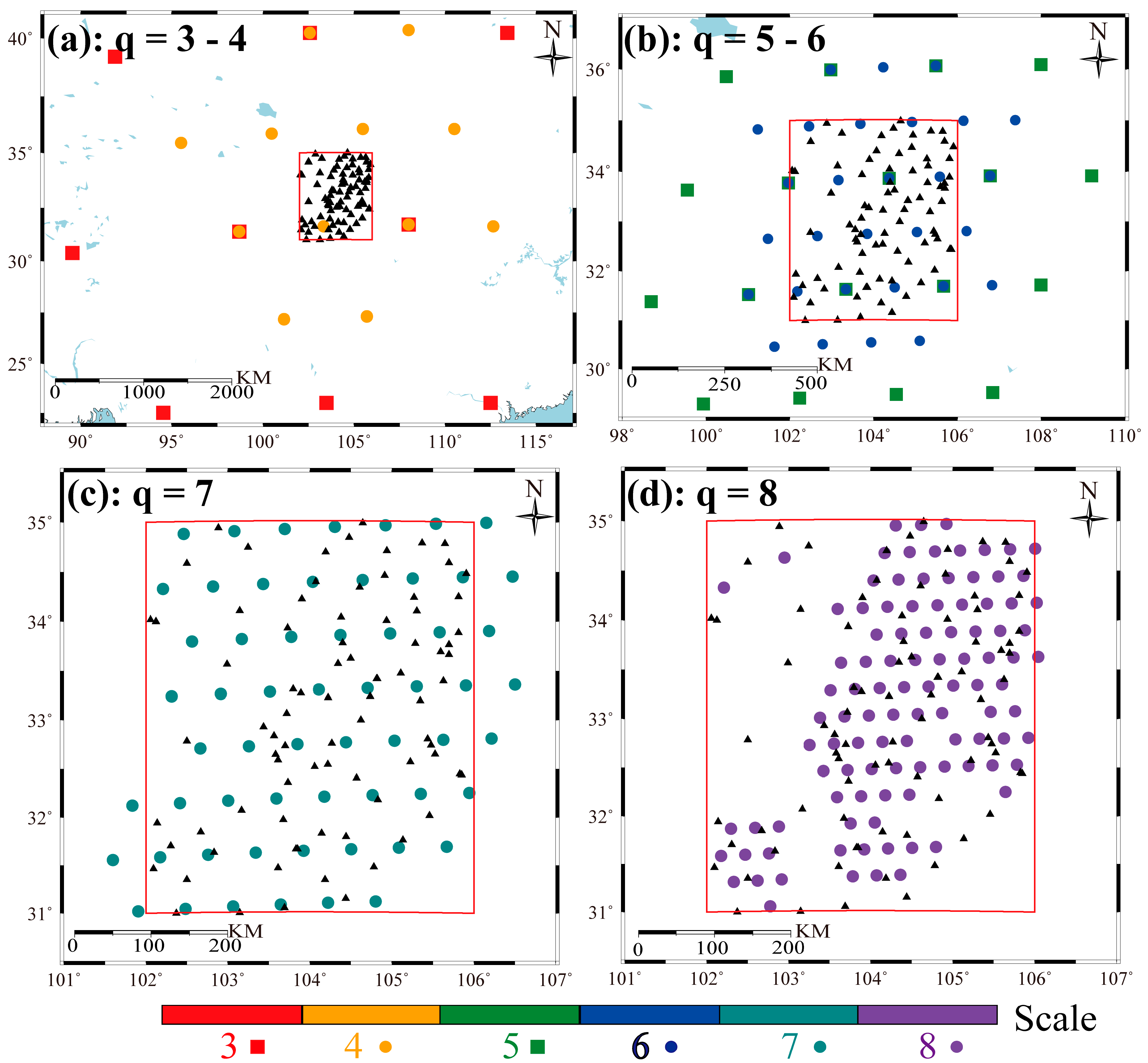
With the scale ranging between three and eight, we present the spatial distribution of centers for multiscale spherical wavelet basis functions in Figure 6, with the total number of wavelet basis functions being 231 as sampling interval being 0.2° × 0.2°. Individually, there are 10, 12, 18, 29, 59, and 103 wavelet basis functions for the scales of 3, 4, 5, 6, 7, and 8, respectively. As small scales (q = 3–5) have large spatial coverage (see Figure 1 in Tape et al. [39]), most centers of these basis functions are sparsely distributed outside of the study area, while for large scales (q = 6–8), most centers are concentrated in the rectangle area with larger scales having denser distributions, indicating their ability on depicting subtle information.
5.1.2. Fitting of the Velocity Field
The 2D GPS velocity field on a sphere can be expressed by [36]:
where and are latitude and longitude of the specified GPS site, respectively, is unit vector of the NS direction and is the unit vector of the EW direction, respectively, is the observational velocity vector, and are corresponding scalar functions on the NS and EW direction, respectively. Substituting the scalar functions with spherical wavelet basis functions, then Equation (3) can be written as:
where is the kth DOG wavelet basis function for the GPS site at , and are modeled parameters. By decomposing Equation (4) into individual components at , it leads to:
where and are noisy observations, and denote the measurement noises on the NS and EW components, respectively.
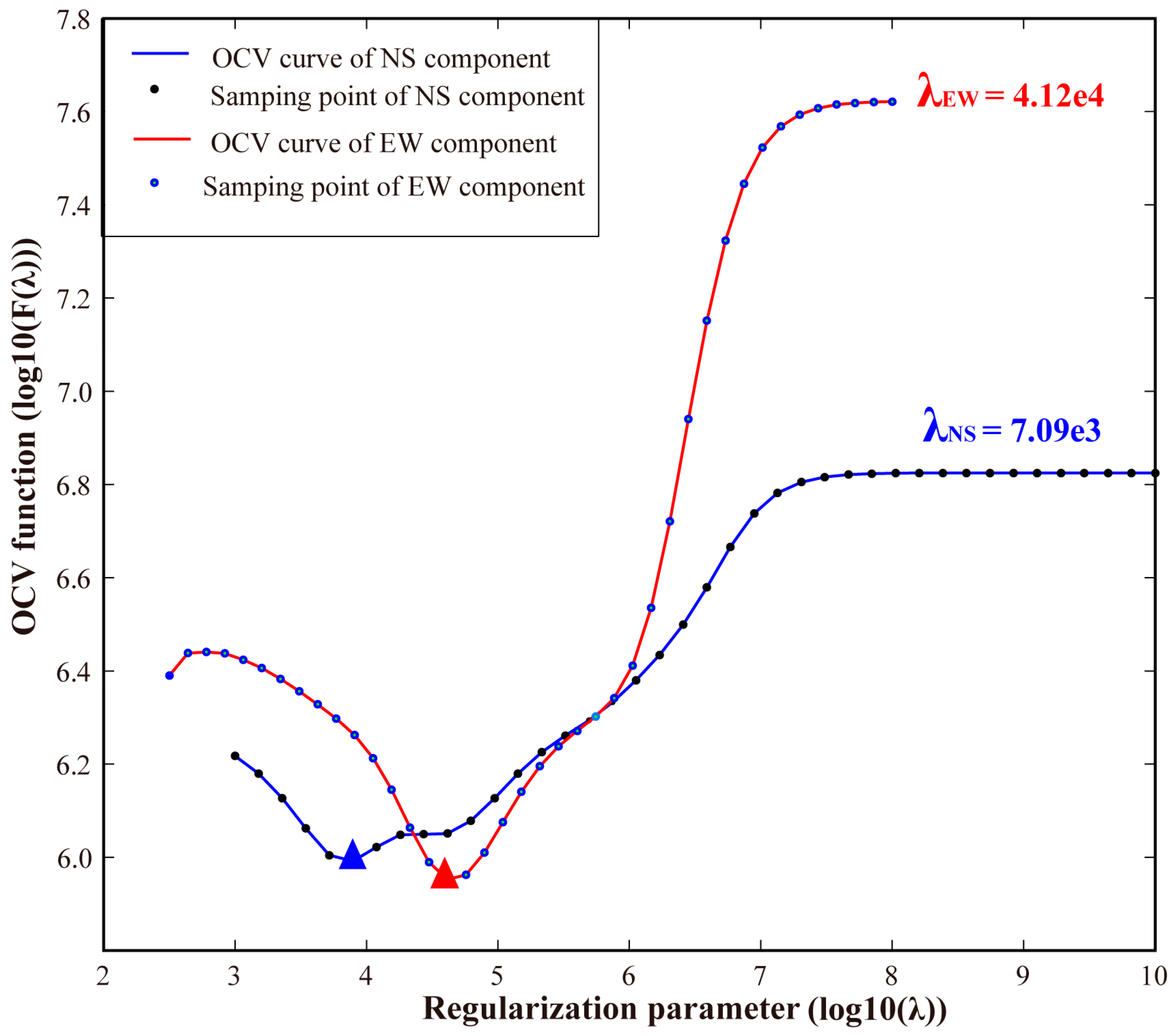
As the DOG wavelet basis functions are derived from the translation and expansion of their mother functions (Equation (1)), they are non-orthogonal, resulting in rank deficiency of the normal equation obtained from the least squares adjustment of Equation (5) [39]. The Tikhonov regularization [42] was applied to controlling the trade-off between the data fit and smoothness of the solution to address this issue (see Equation (B8) in Tape et al. [39]). On the implementation of the Tikhonov regularization, the ordinary cross-validation (OCV) method [43] was employed to determine the regularization parameters. The regularization parameters were determined by searching for the minimum values of OCV functions for EW and NS velocity components, respectively. The OCV function can be expressed as [43]:
where is the index of GPS sites, is the total number GPS sites, is the regularization parameter, is the diagonal element of the regularized data resolution matrix, is the design wavelet basis function matrix with being the kth wavelet basis function of the GPS site at , the superscript represents the matrix transpose, is the estimated value from a model obtained by using all observations, and is the estimated value from a model obtained by using the remaining observations after the ith one being removed. Figure 7 shows the selection of the regularization parameters in the fitting of the GPS velocities. The optimized regularization parameters are 4.12 × 10⁴ and 7.09 × 10³ for the EW and NS components, respectively.
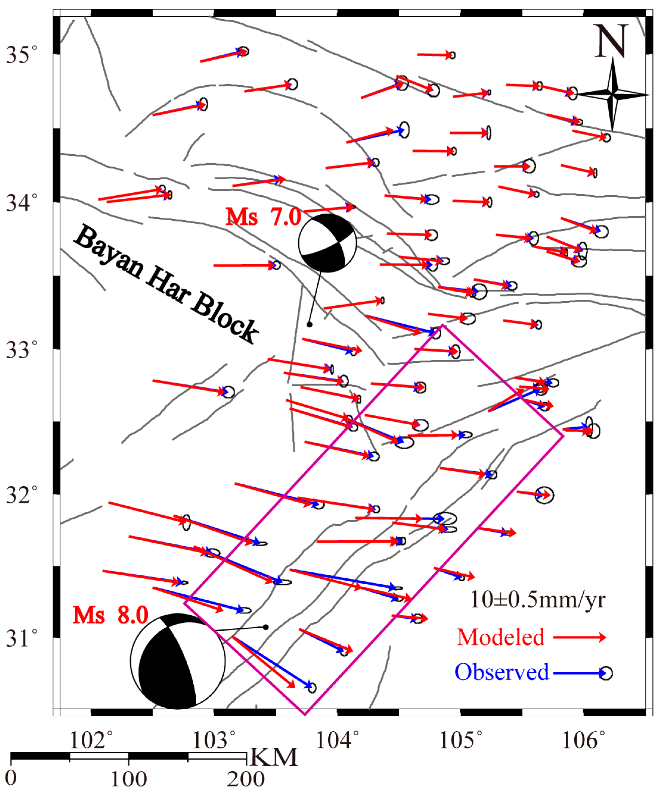
With the Tikhonov regularization on the estimation of modeled parameters, we obtain corresponding modeled velocities through Equation (5). The comparison of the observed and the modeled velocities (Figure 8) shows that the modeled velocities (Table S2) agree well with the observational data except for the southeastern part of the study area (outlined in the pink rectangle), where observed GPS velocities are contaminated by the post-seismic effects of the 2008 Ms 8.0 Wenchuan earthquake. The RMS of the velocity differences is 0.31 mm/y, which is smaller than the mean uncertainties (0.36 mm/y) of the observed GPS velocity field, indicating that the modeled velocity field derived from the multiscale spherical wavelet approach could reflect the observed deformation of the eastern Bayan Har block.
5.1.3. Strain Rates Estimation
The first-order partial differential was performed for the wavelet basis functions, and the components of velocity gradient tensor at a specified point can be expressed as:
where , , and are the components of the velocity gradient tensor, and are the first-order partial differential of the wavelet basis functions in the NS and EW components, respectively, and are estimated parameters for the two components, respectively, expressed as:
With the estimated velocity gradient tensor, strain components at a specified grid point can be expressed as [36]:
where and are EW and NS velocity components at the specific grid point, respectively, is the radius of the Earth.
5.2. GPS Strain Rate Field in the Northeastern Tibetan Plateau
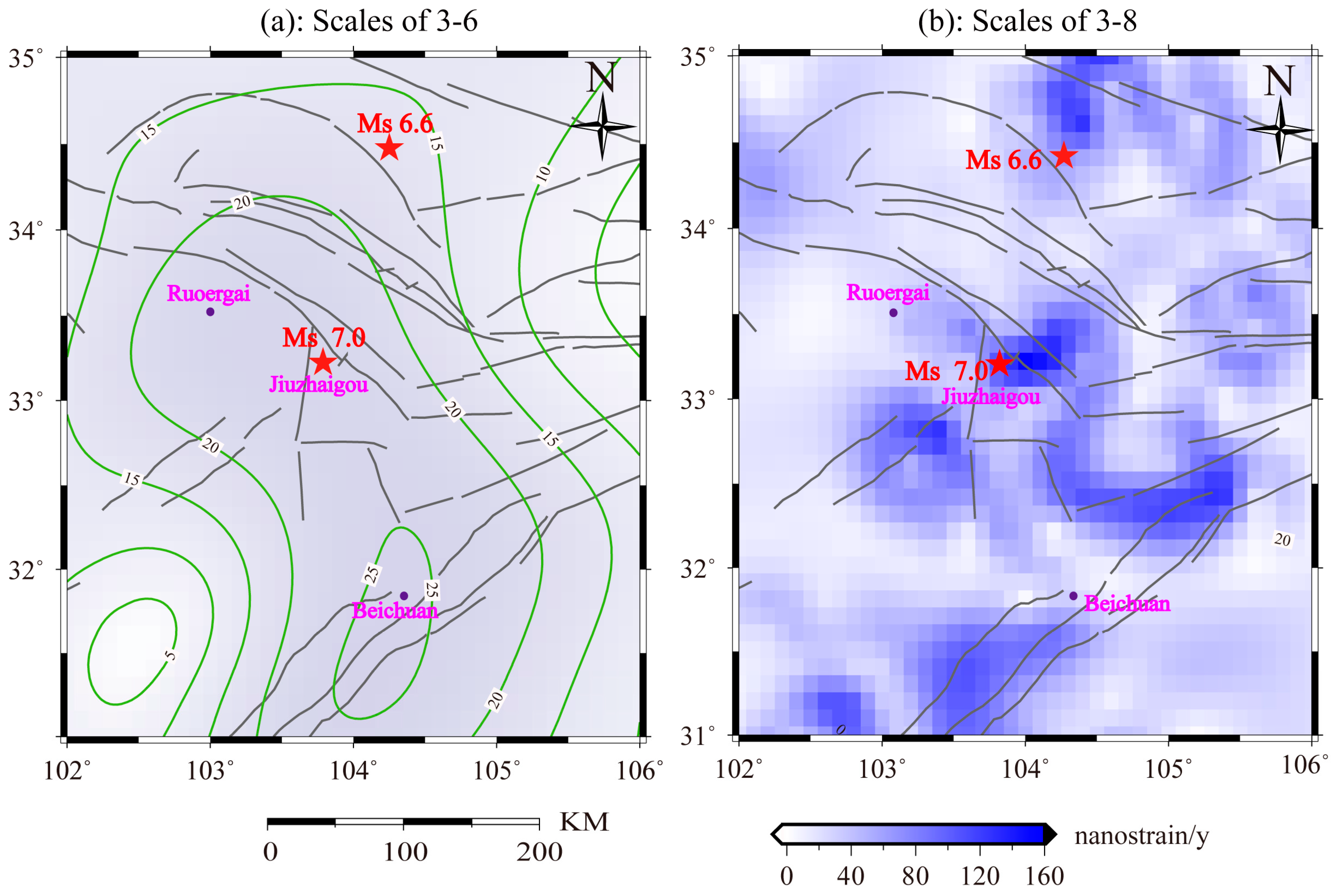
Strain rates at different decomposition scales represent the strain accumulation of different spatial wavelengths. Figure 9 shows the distribution of the maximum shear strain rates in the Northeastern Tibetan Plateau. The strain rate at the scales 3–6 (Figure 9a) represents the strain accumulation of large spatial scale, comprising contributions from the scales of 3-6, which indicates strain rate with the wavelength being from 174 km to 1389.9 km (see Table 3 in Tape et al. [39]). The maximum value of 20–30 nanostrain/y appeared at an elongated zone from Ruoergai to Beichuan nearly in the NS direction. Figure 9b shows the strain rates at the scales of 3–8, which involves the contribution with spatial scales ranging from 43.6 km to 87.2 km [39], other than the contribution from the scales of 3–6. The result demonstrates that localized strain accumulation appeared around the epicentral area of the Jiuzhaigou earthquake, with maximum shear rates being 100–140 nanostrain/y. Moreover, the epicentral area of the 2013 Minxian–Zhangxian Ms 6.6 earthquake also exhibited noticeable localized maximum shear strain rates.
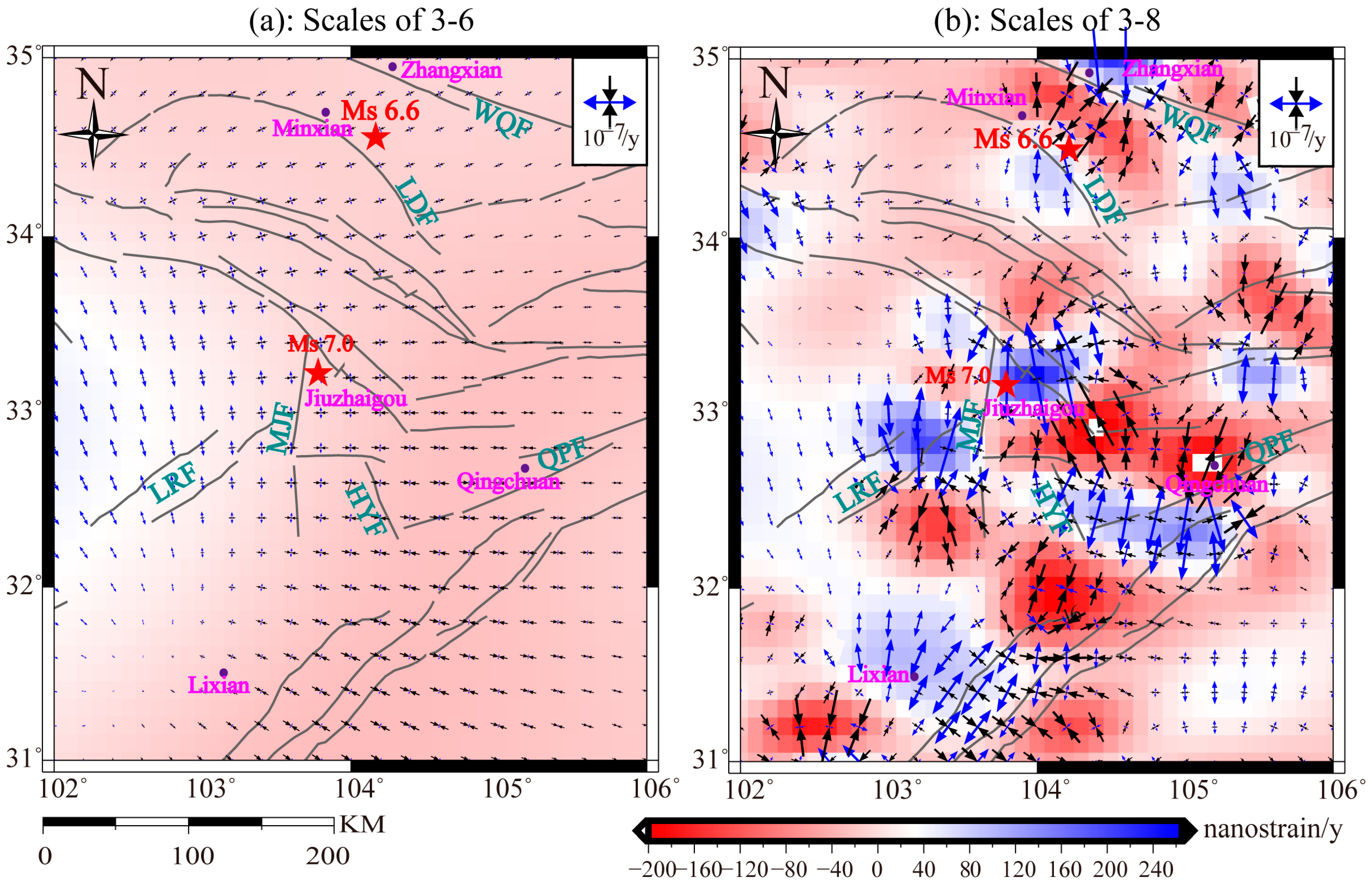
Figure 10 shows the distribution of the principal and dilatation strain rates. The principal and dilatation strain rates at the scales of 3–6 (Figure 10a) show that the region west of the MJF was dominated by near NS extension, and notable dilatation changes (gradually increasing of compressional rate from west to east). However, the region east of the MJF experienced large magnitude of compression, with the principal compression axis being in the near EW direction.
The principal and dilatation strain rates at the scales of 3–8 (Figure 10b) represent a comprehensive contribution from crustal deformation at the scales of 3–6, scale 7, and scale 8. It can be seen that the epicentral zone of the Jiuzhaigou earthquake experienced significant extension, with the maximum extensional strain rate being 100–160 nanostrain/y. In the three regions close to Lixian, Qingchuan, and Minxian, the principal strain and dilation rates were also significant. To the northwest of the LRF, it generally underwent extensional deformation. However localized compression was identified around the southeastern part of the LRF, with an elongated zone in the SE direction. The compression zone between the MJF and HYF coincides with uplift of Minshan Mountain, which is bounded by the MJF in the west and the HYF in the east (Figure 1). The HYF was characterized by left-lateral shear deformation, in agreement with the estimated sinistral slip rate in Section 4. On the both sides of the WQF, the Qingchuan–Pingwu fault (QPF) and the LDF, localized compression and extension were identified in pairs, indicating notable strain accumulation of small scales. Pronounced dilatation rate changes occurred along the HYF, with values switching from positive in the northern extension part to negative in the middle segment and turning back to positive in the south. The epicenter of the Jiuzhaigou earthquake was located at the buffer zone between the compressional and extensional segments of the HYF. In addition, localized compressional deformation was also identified between Minxian and Zhangxian, as well as near Qingchuan.
6. Discussion
6.1. Benefit of the Wavelet-Based Strain Rate Calculation
Various methods were proposed to calculate GPS strain rate. However, the problem is poorly defined due to the non-uniform distribution of GPS sites within the study area [44]. Comparative studies using modeled data showed that different functions used in the strain rate computation might produce varied results even if identical data sets were employed [45], mostly because the adopted parameterization was uniform or quasi-uniform in spatial scale, based on the spacing within a nearly uniform grid of estimation points [46] or based on explicit use of a parameter that weights observational data regarding distance from the specified estimation point [47,48,49].
As crustal deformation occurs at multiple scales in space, a multiscale representation is needed to characterize its spatial characteristics. The multiscale spherical wavelet method has an inherent strength to localize a given deformation field in space and scale as well as to detect outliers in the set of observations [39]. Meanwhile, this method can also locally match the smallest resolved signal to the local spatial density of observational data, maximizing the amount of derived deformation signal and also allowing the comparison of derived signals at the same scale but in different areas [39,41]. In addition, the multiscale spherical wavelet basis function are analytically differentiable, leading to the straightforward computation of the strain rates from the estimated parameters in modeling the observed GPS velocity field (Equation (7)).
6.2. Heterogeneous Strain Buildup in the Northeastern Tibetan Plateau
The multiscale spherical wavelet approach was well suited to study the strain rate in the Northeastern Tibetan Plateau, where crustal deformation was found to be spatially complex due to the inter-connection of multiple faults cutting crust into multiscale tectonic terrains. A cluster of NW (northwest)- and NE-trending conjugate shear faults connects the NS-trending MJF and HYF in this region. These faults are characterized by various geometries and displayed different degrees of activities [7]. The quantitative study on the late Quaternary activity of the major tectonics demonstrated that only a small fraction of left-lateral slip on the TZF was transferred onto the WXF zone, whereas most motion was transformed into nearly NS-striking LRF, MJF, and HYF, south of the TZF, thus leading to the uplift of the Minshan Mountain [15]. The tectonic complexity gives rise to a heterogeneous strain buildup which might be sampled by present-day GPS observations.
On the other hand, GPS sites are unevenly distributed in this region, sampling various spatial scales of crustal deformation. The derived strain rate at the scales of 3–6, with spherical triangular length in the range of 110.2–881.7 km (see Table 1 in Su et al. [41]), mostly represents relatively long wavelength of crustal deformation. This can be seen from the fact that there are no sharp gradients for the maximum shear strain rates in Figure 9a. Dilatation strain rate at the scales of 3–6 demonstrates that compressional deformation is dominant at the eastern zone of the study area, with localized extensional deformation in the west of the MJF, indicating the inherited uplift of the Minshan Mountain (Figure 10a). As shown by Figure 11 and Figure 12, the strain rates at the scales of 7 and 8, with spherical triangular length of 55.1 km and 27.5 km [41], respectively, could reflect localized heterogeneous deformation due to the small scale of tectonic terrains and/or active faults.
6.3. Comparison between Strain Rates and Seismicity
We collected the earthquake catalogue from China Earthquake Data Center (CEDC), which provides the earthquake locus, local magnitude, and seismic phase information free online (http://data.earthquake.cn). We selected Ms > 4.5 earthquakes which occurred after the 2008 Ms 8.0 earthquake in the study area. There were four Ms > 4.5 earthquakes, including the 22 July 2013 Ms 6.6 Minxian–Zhangxian earthquake, the 11 April 2014 Ms 4.8 Lixian earthquake, the 10 June 2014 Ms 4.8 Qingchuan earthquake, and the 8 August 2017 Ms 7.0 Jiuzhaigou earthquake.
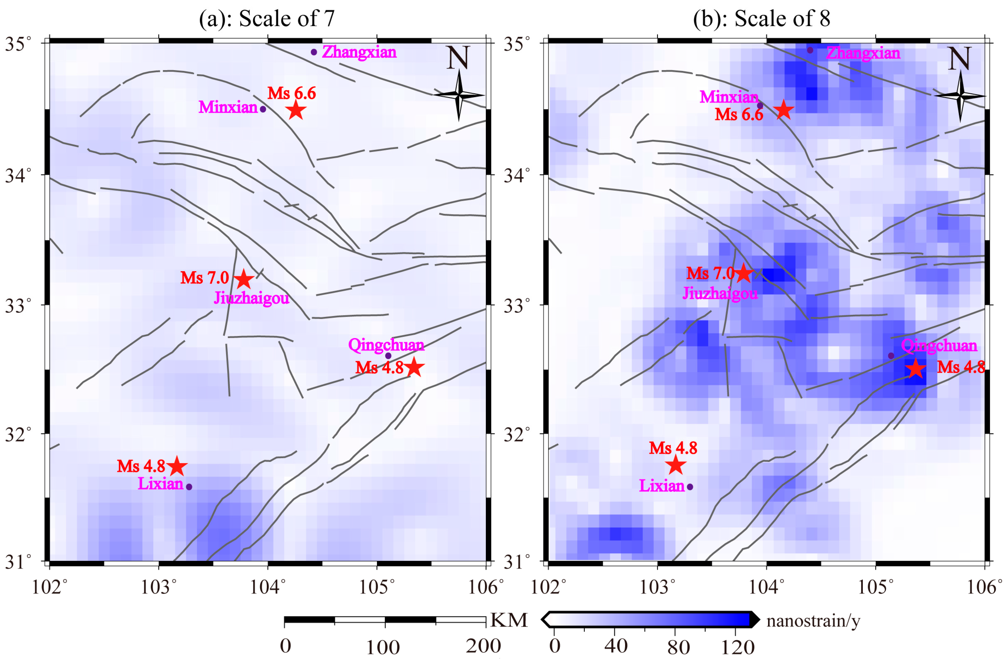
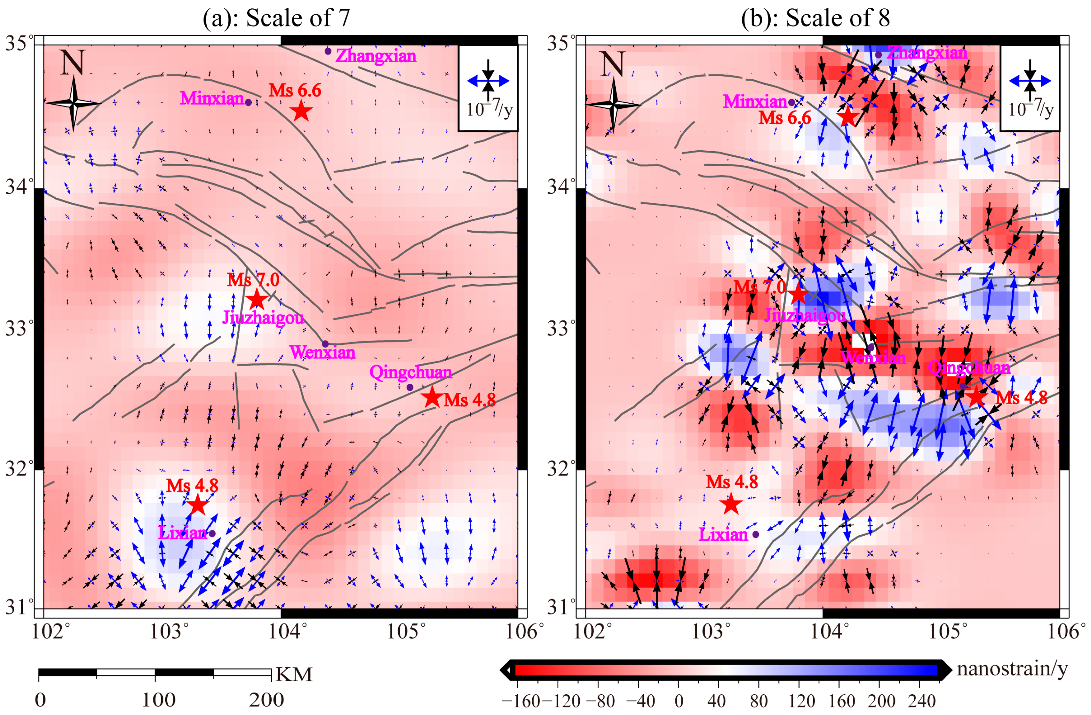
At the decomposition scale of 7 for the maximum shear strain rates (Figure 11a), localized deformation appeared around the Lixian zone, with maximum value reaching ~100 nanostrain/y. However, the rest of the regions displayed insignificant shear strain. At the scale of 8, the maximum shear strain around the Lixian zone was still significant (Figure 11b). Additionally, the broad region was characterized by significant maximum shear strain rate, including the region around the epicenter of the Jiuzhaigou earthquake, with a maximum value being 100–120 nanostrain/y, the region between Minxian and Zhangxian, with a maximum value being 60–120 nanostrain/y, and the region near Qingchuan, with a maximum value being 60–120 nanostrain/y. The localized maximum shear strain around the Lixian Ms 4.8 and the Qingquan Ms 4.8 earthquakes were possibly due to the post-seismic deformation of the 2008 Wenchuan Ms 8.0 earthquake.
The principal and dilatation strain rates at the scale of 7 (Figure 12a) show that maximum extensional deformation appeared near Lixian, reaching ~80 nanostrain/y. Compressional deformation dominated in an elliptical zone with a major axis nearly perpendicular to the LMF. Another compressional zone was identified around Jiuzhaigou. In the northeastern segment of the LMF, the principal strain rates perpendicular to the fault exhibited compressional deformation; strain rates parallel to the fault were dominated by extension. This strain pattern agrees with previous a study showing that the northeastern segment of the LMF exhibited compressional and right lateral shear deformation after the 2008 Ms 8.0 Wenchuan earthquake [50].
The principal and dilatation rate at the scale of 8 (Figure 12b) demonstrates that significant extension occurred at the epicentral zone of the Jiuzhaigou earthquake, with a maximum value being ~160 nanostrain/y. The principal strain rate (Figure 12b) shows significant extension in the NW–SE (northwest-southeast) direction. Localized compression rates were found near the epicentral zone of the 2013 Ms 6.6 Minxian–Zhangxian earthquake. The epicenter of this earthquake was also located between a localized extension zone to the south and a localized compression zone to the north, which has a similar pattern compared to the Jiuzhaigou earthquake. In addition, significant localized principal and dilatation strain rates were also identified near the Lixian area, where an Ms 4.8 earthquake occurred on 11 April 2014, and Qingchuan area, where another Ms 4.8 earthquake occurred on 10 June 2014. As these areas are located close to the rupture belt of the 2008 Ms 8.0 Wenchuan earthquake, the estimated GPS velocities were enlarged (Figure 3) by the post-seismic effects of the large earthquake, and the fitting of multiscale wavelet functions were defective (Figure 8), thus inferring inaccurate strain rate estimation around the LMF zone. Therefore, the significant localized strain rate was possibly due to the post-seismic relaxation of the large earthquake.
7. Conclusions
Using GPS data at 81 continuous and repeatedly surveyed campaign sites in the northeastern borderland of the Tibetan Plateau over the period of 2009–2017, we characterized the crustal deformation prior to the 2017 Jiuzhaigou Ms 7.0 earthquake, the largest earthquake after the 2008 Wenchuan Ms 8.0 earthquake in this region. The velocity field shows a noticeable decrease, from the west of the epicenter of the Jiuzhaigou earthquake to the western edge of LMF, in the southeast direction. The total NWW–SEE (northwest west-southeast east) shortening rate in the vicinity of the epicentral area of the Jiuzhaigou earthquake is in the range of 1.5 mm/y to 3.1 mm/y. We estimated the motion of the HYF with a dominant left-lateral slip rate being 3.3 ± 0.2 mm/y.
Multiscale components of the 2D strain rate tensor show a complex deformation pattern due to the clustering of NW- and NE-trending conjugate shear faults, which connect the NS-trending MJF and HYF. The maximum shear rates reveal that the Jiuzhaigou earthquake occurred at the buffer zone between extensional and compressional deformation, and with significant localized shear rates being 100–140 nanostrain/y. Compressional strain was identified around the HYF in the middle segment; however, extensional strain was detected around the northern extension of the fault. Moreover, a maximum shear strain rate of 60–120 nanostrain/y appeared near the epicenter of the 2013 Ms 6.6 Minxian–Zhangxian earthquake. Given the high frequency of medium- and large-sized earthquakes on the northeastern margin of the Tibetan Plateau, the construction of more continuous GPS sites are justified in order to acquire a higher resolution of crustal deformation to identify strain buildup related to future earthquakes in this region.
Supplementary Materials
The following are available online at https://www.mdpi.com/2072-4292/10/12/2028/s1, Figure S1: Coordinate time-series of involved GPS sites; Table S1: GPS velocities; Table S2: Modeled velocities based on multiscale wavelet method.
Author Contributions
W.W. and G.M. initialized the idea and drafted the manuscript. X.S. and C.L. participated in the design of the study and helped to draft the manuscript. G.M. helped to revise the manuscript.
Funding
This research was funded by the National Natural Science Foundation of China grant number 41611530702, 41604007, 41674003 and 41874024, the National Basic Research Program of China/973 Project grant number 2013CB733304, the International Science and Technology Cooperation Program of China grant number 2015DFR21100, and the Fundamental Research Project of Institute of Earthquake Forecasting, China Earthquake Administration grant number 2016IES102.
Acknowledgments
We are grateful for Data Center of CMONOC for providing GPS observations. Partial figures are drawn using GMT software.
Conflicts of Interest
The authors declare no conflict of interest.
References
- Molnar, P.; Tapponnier, P. Cenozoic Tectonics of Asia: Effects of a Continental Collision: Features of recent continental tectonics in Asia can be interpreted as results of the India-Eurasia collision. Science 1975, 189, 419–426. [Google Scholar] [CrossRef] [PubMed]
- Tapponnier, P.; Molnar, P. Active faulting and tectonics in China. J. Geophys. Res. 1997, 82, 2905–2930. [Google Scholar] [CrossRef]
- Tapponnier, P.; Zhiqin, X.; Roger, F.; Meyer, B.; Arnaud, N.; Wittlinger, G.; Jingsui, Y. Oblique stepwise rise and growth of the Tibet plateau. Science 2001, 294, 1671–1677. [Google Scholar] [CrossRef] [PubMed]
- Hubbard, J.; Shaw, J.H. Uplift of the Longmen Shan and Tibetan plateau, and the 2008 Wenchuan (M = 7.9) earthquake. Nature 2009, 458, 194. [Google Scholar] [CrossRef] [PubMed]
- Clark, M.K.; Royden, L.H. Topographic ooze: Building the eastern margin of Tibet by lower crustal flow. Geology 2000, 28, 703–706. [Google Scholar] [CrossRef]
- Royden, L.H.; Burchfiel, B.C.; van der Hilst, R.D. The geological evolution of the Tibetan Plateau. Science 2008, 321, 1054–1058. [Google Scholar] [CrossRef] [PubMed]
- Chen, C.Y.; Ren, J.W.; Meng, G.J.; Yang, P.X.; Xiong, R.W.; Hu, C.Z.; Su, X.N.; Su, J.F. Division, deformation and tectonic implication of active blocks in the eastern segment of Bayan Har block. Chin. J. Geophys. 2013, 56, 4125–4141. [Google Scholar] [CrossRef]
- Ren, J.W.; Xu, X.W.; Yeats, R.S.; Zhang, S.M. Latest Quaternary paleoseismology and slip rates of the Longriba fault zone, eastern Tibet: Implications for fault behavior and strain partitioning. Tectonics 2013, 32, 216–238. [Google Scholar] [CrossRef] [Green Version]
- Shen, Z.K.; Lü, J.; Wang, M.; Bürgmann, R. Contemporary crustal deformation around the southeast borderland of the Tibetan Plateau. J. Geophys. Res. 2005, 110, B11409. [Google Scholar] [CrossRef]
- Yi, G.X.; Long, F.; Liang, M.J.; Zhang, H.P.; Zhao, M.; Ye, Y.Q.; Zhang, Z.W.; Qi, Y.P.; Wang, S.W.; Gong, Y.; et al. Focal mechanism solutions and seismogenic structure of the 8 August 2017 M7 Jiuzhaigou earthquake and its aftershocks, northern Sichuan. Chin. J. Geophys. 2017, 60, 4083–4097. [Google Scholar] [CrossRef]
- Fang, L.H.; Wu, J.P.; Su, J.R.; Wang, M.M.; Jiang, C.; Fan, L.P.; Wang, W.L.; Wang, C.Z.; Tan, X.L. Relocation of mainshock and aftershock sequence of the Ms7.0 Sichuan Jiuzhaigou earthquake. Chin. Sci. Bull. 2018, 63, 649–662. [Google Scholar] [CrossRef]
- Kirby, E.; Whipple, K.X.; Burchfiel, B.C.; Tang, W.; Berger, G.; Sun, Z.; Chen, Z. Neotectonics of the Min Shan, China: Implications for mechanisms driving Quaternary deformation along the eastern margin of the Tibetan Plateau. Geol. Soc. Am. Bull. 2000, 112, 375–393. [Google Scholar] [CrossRef]
- Deng, Q.D.; Zhang, P.Z.; Ran, Y.K.; Yang, X.P.; Min, W.; Chu, Q.Z. Basic characteristics of active tectonics of China. Sci. Chin. Ser. D-Earth Sci. 2003, 46, 356–372. [Google Scholar] [CrossRef]
- Densmore, A.L.; Ellis, M.A.; Li, Y.; Zhou, R.; Hancock, G.S.; Richardson, N. Active tectonics of the Beichuan and Pengguan faults at the eastern margin of the Tibetan Plateau. Tectonics 2007, 26, TC4005. [Google Scholar] [CrossRef]
- Ren, J.J.; Xu, X.W.; Zhang, S.M.; Luo, Y.; Liang, O.B.; Zhao, J.X. Tectonic transformation at the eastern termination of the eastern Kunlun fault zone and seismogenic mechanism of the 8 August 2017 Jiuzhaigou Ms 7.0 earthquake. Chin. J. Geophys. 2017, 60, 4027–4045. [Google Scholar] [CrossRef]
- Sun, J.B.; Yue, H.; Shen, Z.K.; Fang, L.H.; Zhan, Y.; Sun, X.Y. The 2017 Jiuzhaigou earthquake: A complicated event occurred in a young fault system. Geophys. Res. Lett. 2018, 45, 2230–2240. [Google Scholar] [CrossRef]
- Wen, X.Z.; Du, F.; Zhang, P.Z.; Long, F. Correlation of major earthquake sequences on the northern and eastern boundaries of the Banyan Har block, and its relation to the 2008 Wenchuan earthquake. Chin. J. Geophys. 2011, 54, 706–716. [Google Scholar] [CrossRef]
- Xu, X.W.; Chen, G.H.; Wang, Q.X.; Chen, L.C.; Ren, Z.K.; Xu, C.; Wei, Z.Y.; Lu, R.Q.; Tan, X.B.; Dong, S.P.; et al. Discussion on seismogenic structure of Jiuzhaigou earthquake and its implication for current strain state in the southeastern Qinghai-Tibet Plateau. Chin. J. Geophys. 2017, 60, 4018–4026. [Google Scholar] [CrossRef]
- Herring, T.A.; King, R.W.; Floyd, M.A.; McClusky, S.C. Introduction to GAMIT/GLOBK, Release 10.6; Massachusetts Institute of Technology: Cambridge, MA, USA, 2015. [Google Scholar]
- Rebischung, P.; Altamimi, Z.; Ray, J.; Garayt, B. The IGS contribution to ITRF2014. J. Geod. 2016, 90, 611–630. [Google Scholar] [CrossRef]
- Zhang, Z.Y.; Guo, F.; Zhang, X.H. The effects of higher-order ionospheric terms on GPS tropospheric delay and gradient estimates. Remote Sens. 2018, 10, 1561. [Google Scholar] [CrossRef]
- Petrie, E.J.; King, M.A.; Moore, P.; Lavalle´e, D.A. Higher-order ionospheric effects on the GPS reference frame and velocities. J. Geophys. Res. 2010, 115, B03417. [Google Scholar] [CrossRef]
- Zus, F.; Dick, G.; Dousa, J.; Wickert, J. Systematic errors of mapping functions which are based on the VMF1 concept. GPS Solut. 2015, 19, 277–286. [Google Scholar] [CrossRef]
- Figurski, M.; Nykiel, G. Investigation of the Impact of ITRF2014/IGS14 on the Positions of the Reference Stations in Europe. Acta Geodyn. Geomater. 2017, 14, 401–410. [Google Scholar] [CrossRef]
- Lagler, K.; Schindelegger, M.; Böhm, J.; Krásná, H.; Nilsso, T. GPT2: Empirical slant delay model for radio space geodetic techniques. Geophys. Res. Lett. 2013, 40, 1069–1073. [Google Scholar] [CrossRef] [PubMed] [Green Version]
- Lyard, F.; Lefevre, F.; Letellier, T.; Francis, O. Modelling the global ocean tides: modern insights from FES2004. Ocean Dyn. 2006, 56, 394–415. [Google Scholar] [CrossRef]
- Li, Z.; Yue, J.P.; Hu, J.Y.; Xiang, Y.F.; Chen, J.; Bian, Y.K. Effect of surface mass loading on geodetic GPS observations. Appl. Sci. 2018, 8, 1851. [Google Scholar] [CrossRef]
- Altamimi, Z.; Rebischung, P.; Metivier, L.; Collilieux, X. ITRF2014: A new release of the International Terrestrial Reference Frame modeling nonlinear station motions. J. Geophys. Res. 2016, 121, 6108–6131. [Google Scholar] [CrossRef]
- Su, X.N.; Meng, G.J.; Sun, H.L.; Wu, W.W. Positioning Performance of BDS Observation of the Crustal Movement Observation Network of China and Its Potential Application on Crustal Deformation. Sensors 2018, 18, 3353. [Google Scholar] [CrossRef]
- Williams, S.D.P.; Bock, Y.; Fang, P.; Jamason, P.; Nikolaidis, R.M.; Prawirodirdjo, L.; Miller, M.; Johnson, D.J. Error analysis of continuous GPS position time series. J. Geophys. Res. 2004, 109, B03412. [Google Scholar] [CrossRef]
- Bos, M.S.; Fernandes, R.M.S.; Williams, S.D.P.; Bastos, L. Fast error analysis of continuous GNSS observations with missing data. J. Geod. 2013, 87, 351–360. [Google Scholar] [CrossRef]
- Altamimi, Z.; Métivier, L.; Rebischung, P.; Rouby, H.; Collilieux, X. ITRF2014 Plate Motion Model. Geophys. J. Int. 2017, 209, 1906–1912. [Google Scholar] [CrossRef]
- Meade, B.J.; Hager, B.H. Block models of crustal motion in southern California constrained by GPS measurements. J. Geophys. Res. 2005, 110, B03403. [Google Scholar] [CrossRef]
- Meade, B.J. Present-day kinematics at the India-Asia collision zone. Geology 2007, 35, 81–84. [Google Scholar] [CrossRef]
- McCaffrey, R.; Qamar, A.I.; King, R.W.; Wells, R.; Khazaradze, G.; Williams, C.A.; Stevens, C.W.; Vollick, J.J.; Zwick, P.C. Fault locking, block rotation and crustal deformation in the Pacific Northwest. Geophys. J. Int. 2007, 169, 1315–1340. [Google Scholar] [CrossRef] [Green Version]
- Savage, J.C.; Gan, W.J.; Svarc, J.L. Strain accumalation and rotation in the Eastern California Shear Zone. J. Geophys. Res. 2001, 106, 21995–22007. [Google Scholar] [CrossRef]
- Hardy, R.L.; Göpfert, W.M. Least squares prediction of gravity anomalies, geoidal undulations, and deflections of the vertical with multiquadric harmonic functions. Geophys. Res. Lett. 1975, 2, 423–426. [Google Scholar] [CrossRef]
- Kahle, H.G.; Cocard, M.; Peter, Y.; Geiger, A.; Reilinger, R.; Barka, A.; Veis, G. GPS-derived strain rate field within the boundary zones of the Eurasian, african, and arabian plates. J. Geophy. Res. 2000, 105, 23353–23370. [Google Scholar] [CrossRef]
- Tape, C.; Pablo, M.; Simons, M.; Dong, D.; Webb, F. Multiscale estimation of GPS velocity fields. Geophys. J. Int. 2009, 179, 945–971. [Google Scholar] [CrossRef] [Green Version]
- Bogdanova, I.; Vandergheynst, P.; Antoine, J.P.; Jacques, L.; Morvidone, M. Stereographic wavelet frames on the sphere. Appl. Comput. Harmon. A 2005, 19, 223–252. [Google Scholar] [CrossRef]
- Su, X.N.; Meng, G.J.; Wang, Z. Methodology and application of GPS strain field estimation based on spherical wavelet. Chin. J. Geophys. 2016, 59, 1585–1595. [Google Scholar]
- Golub, G.H.; Hansen, P.C.; O’Leary, D.P. Tikhonov Regularization and Total Least Squares. Siam J. Matrix Anal. Appl. 1997, 21, 185–194. [Google Scholar] [CrossRef]
- Golub, G.H.; Wahba, H.G. Generalized cross-validation as a method for choosing a good ridge parameter. Technometrics 1979, 21, 215–223. [Google Scholar] [CrossRef]
- Allmendinger, R.W.; Reilinger, R.; Loveless, J. Strain and rotation rate from GPS in Tibet, Anatolia, and the Altiplano. Tectonics 2007, 26, TC3013. [Google Scholar] [CrossRef]
- Wu, Y.Q.; Jiang, Z.S.; Yang, G.H.; Wei, W.X.; Liu, X.X. Comparison of GPS strain rate computing methods and their reliability. Geophys. J. Int. 2011, 185, 703–717. [Google Scholar] [CrossRef] [Green Version]
- Beavan, J.; Haines, J. Contemporary horizontal velocity and strain rate fields of the Pacific-Australian plate boundary zone through New Zealand. J. Geophys. Res. 2001, 10, 741–770. [Google Scholar] [CrossRef]
- Shen, Z.K.; Jackson, D.D.; Ge, B.X. Crustal deformation across and beyond the Los Angeles basin from geodetic measurements. J. Geophys. Res. 1996, 101, 27957–27980. [Google Scholar] [CrossRef] [Green Version]
- Ward, S.N. On the consistency of earthquake moment rates, geological fault data, and space geodetic strain: The United States. Geophys. J. Int. 1998, 134, 172–186. [Google Scholar] [CrossRef]
- Hsu, Y.J.; Yu, S.B.; Simons, M.; Kuo, L.C.; Chen, H.Y. Interseismic crustal deformation in the Taiwan plate boundary zone revealed by GPS observations, seismicity, and earthquake focal mechanisms. Tectonophysics 2009, 479, 4–18. [Google Scholar] [CrossRef]
- Meng, G.J.; Su, X.N.; Wu, W.W.; Ren, J.W.; Yang, Y.L.; Wu, J.C.; Chen, C.H.; Shestakov, N.V. Heterogeneous strain regime in the eastern margin of Tibetan Plateau and its tectonic implications. Earthq. Sci. 2015, 28, 1–10. [Google Scholar] [CrossRef] [Green Version]
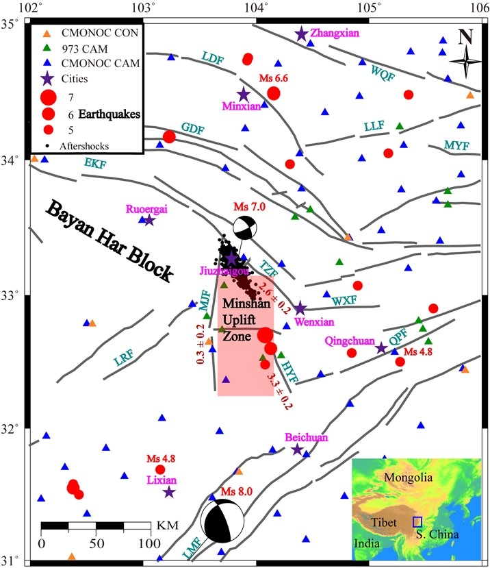
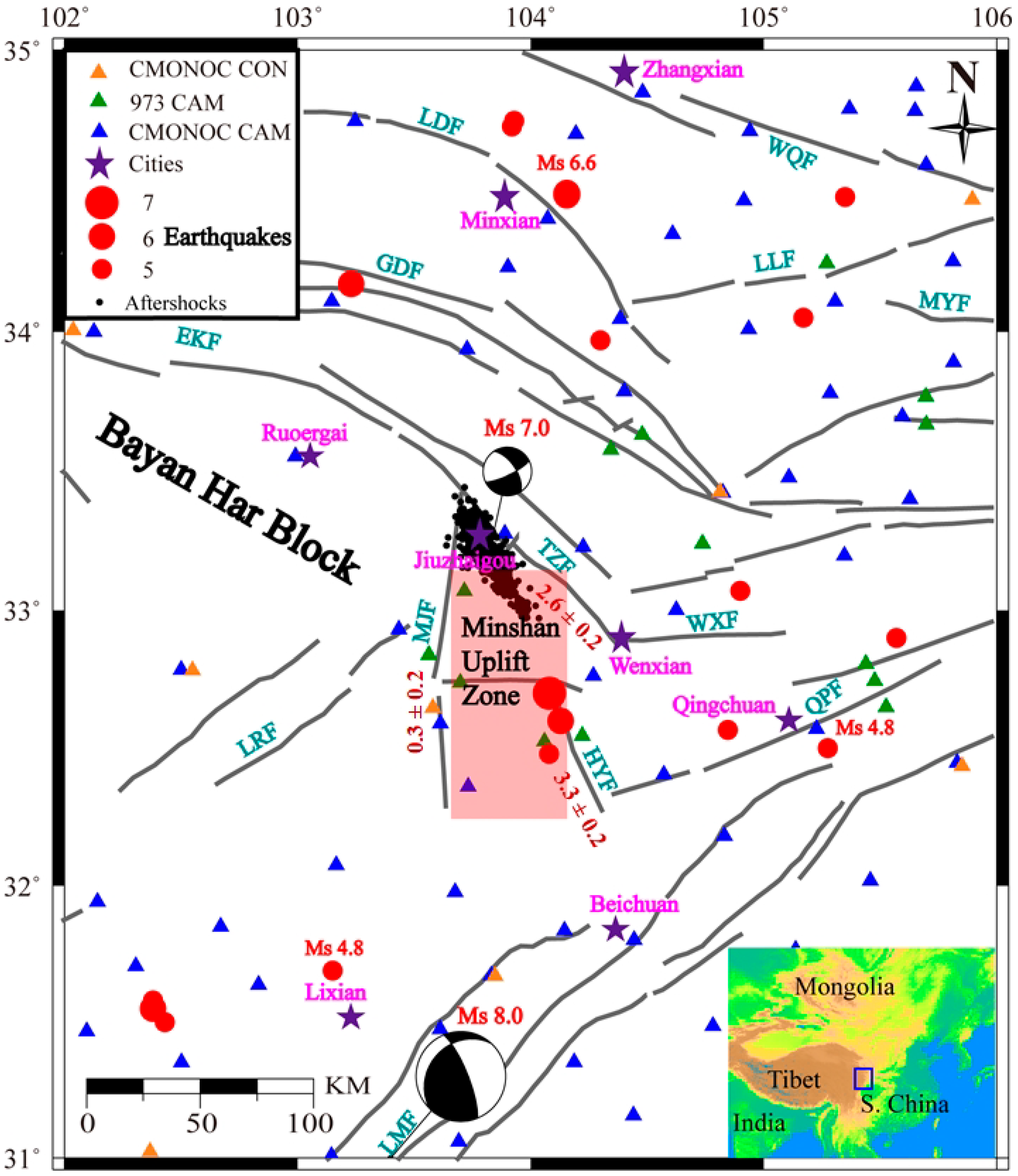
Figure 1.
Distribution of GPS (Global Positioning System) sites and seismicities in the northeastern Bayan Har block. Green triangles are campaign GPS sites of the 973 Project; yellow and blue triangles denote continuous and campaign sites of the Crustal Movement Observation Network of China (CMONOC), respectively. Red dots indicate earthquake events Ms ≥ 4.5 since 1976, exclusive of aftershocks of the 2008 Wenchuan Ms 8.0 earthquake. The beach balls are the focal mechanisms of the Ms 7.0 Jiuzhaigou and Ms 8.0 Wenchuan earthquake, respectively. Black dots are aftershocks of the Ms 7.0 Jiuzhaigou earthquake, with their sizes proportional to event magnitudes. Red words signify recent earthquakes. Purple stars and magenta words show the location of major cities and their names. Cyan capital letters are abbreviations of regional active faults, with EKF being East Kunlun fault zone, GDF being Guanggaushan–Dieshan fault zone, HYF being Huya fault, LDF being Lintan–Dangchang fault, LLF being Lixian–Luojiapu fault, LMF being Longmenshan fault zone, LRF being Longriba fault zone, MJF being Minjiang fault zone, MYF being Mayanhe fault, QPF being Qingchuan–Pingwu fault zone, TZF being Tazang fault, WQF being West Qingling North fault zone, WXF being Wenxian fault. Pink rectangle zone is general region of the Minshan Uplift Zone. Brown numbers are the estimated strike-slip rates in unit of mm/y for the HYF, MJF, and TZF, with positive values denoting left-lateral.

Figure 2.
Time occupation history of GPS sites. (a) Continuous sites from CMONOC; (b) campaign sites from CMONOC; (c) campaign sites from the 973 Project.
Figure 2.
Time occupation history of GPS sites. (a) Continuous sites from CMONOC; (b) campaign sites from CMONOC; (c) campaign sites from the 973 Project.

Figure 3.
GPS velocity field over the period of 2009–2017. (a) GPS velocity relative to the stable Eurasian plate. Pink rectangles (T1, T2, and T3) are three GPS velocity profiles for the MJF, HYF, and TZF, respectively; (b) GPS velocity with respect to the stable South China block. Error ellipses are 95% confidence interval. The beach balls are the focal mechanisms of the Ms 7.0 Jiuzhaigou and Ms 8.0 Wenchuan earthquake, respectively.

Figure 4.
GPS velocity transects: (a) fault-parallel (sinistral positive) velocity component and (b) fault-normal velocity (extensional positive) component with respect to the distance from the MJF, HYF, and TZF along transects outlined as T1, T2, and T3 in Figure 3. Error bars represent one sigma of the estimated velocities.

Figure 5.
The maximum value of the scale factor. Black triangles are GPS sites.

Figure 6.
Spatial distribution of centers for multiscale spherical wavelet basis functions: (a) is for q = 3–4; (b) is for q = 5–6; (c) is for q = 7; (d) is for q = 8. Black triangles are positions of GPS sites. Colored dots and squares are centers for wavelet basis functions. Red rectangle outlines the study area.

Figure 7.
Selection of regularization parameters based on the ordinary cross validation (OCV) function. Blue and red solid triangles are preferred values for north–south (NS) and east–west (EW) velocity components, respectively.
Figure 7.
Selection of regularization parameters based on the ordinary cross validation (OCV) function. Blue and red solid triangles are preferred values for north–south (NS) and east–west (EW) velocity components, respectively.

Figure 8.
Comparison between observed and modeled velocity fields. Blue and red arrows represent observed and modeled velocities, respectively. The pink rectangle outlines the region with the largest velocity residuals. The beach balls are the focal mechanisms of the Ms 7.0 Jiuzhaigou and Ms 8.0 Wenchuan earthquake, respectively.

Figure 9.
Maximum shear strain rates at (a) the scales of 3–6 and (b) the scales of 3–8. Red stars depict the epicenters of the 2013 Ms 6.6 Minxian–Zhangxian earthquake and the 2017 Ms 7.0 Jiuzhaigou earthquake.
Figure 9.
Maximum shear strain rates at (a) the scales of 3–6 and (b) the scales of 3–8. Red stars depict the epicenters of the 2013 Ms 6.6 Minxian–Zhangxian earthquake and the 2017 Ms 7.0 Jiuzhaigou earthquake.

Figure 10.
Principal and dilatation strain rates at (a) the scales of 3–6 and (b) the scales of 3–8. Other items are the same as Figure 9.
Figure 10.
Principal and dilatation strain rates at (a) the scales of 3–6 and (b) the scales of 3–8. Other items are the same as Figure 9.

Figure 11.
Maximum shear strain rates at (a) the scale7 and (b) the scale 8. Other items are the same as Figure 9.
Figure 11.
Maximum shear strain rates at (a) the scale7 and (b) the scale 8. Other items are the same as Figure 9.

Figure 12.
Principal and dilatation strain rates at (a) the scale 7 and (b) the scale 8. Other items are the same as Figure 9.
Figure 12.
Principal and dilatation strain rates at (a) the scale 7 and (b) the scale 8. Other items are the same as Figure 9.

© 2018 by the authors. Licensee MDPI, Basel, Switzerland. This article is an open access article distributed under the terms and conditions of the Creative Commons Attribution (CC BY) license (http://creativecommons.org/licenses/by/4.0/).
Share and Cite
MDPI and ACS Style
Wu, W.; Su, X.; Meng, G.; Li, C. Crustal Deformation Prior to the 2017 Jiuzhaigou, Northeastern Tibetan Plateau (China), Ms 7.0 Earthquake Derived from GPS Observations. Remote Sens. 2018, 10, 2028. https://doi.org/10.3390/rs10122028
AMA Style
Wu W, Su X, Meng G, Li C. Crustal Deformation Prior to the 2017 Jiuzhaigou, Northeastern Tibetan Plateau (China), Ms 7.0 Earthquake Derived from GPS Observations. Remote Sensing. 2018; 10(12):2028. https://doi.org/10.3390/rs10122028
Chicago/Turabian StyleWu, Weiwei, Xiaoning Su, Guojie Meng, and Chentao Li. 2018. "Crustal Deformation Prior to the 2017 Jiuzhaigou, Northeastern Tibetan Plateau (China), Ms 7.0 Earthquake Derived from GPS Observations" Remote Sensing 10, no. 12: 2028. https://doi.org/10.3390/rs10122028
Note that from the first issue of 2016, this journal uses article numbers instead of page numbers. See further details here.