Article

Remote Estimation of Nitrogen Vertical Distribution by Consideration of Maize Geometry Characteristics

1
Key Laboratory of Digital Earth Science, Institute of Remote Sensing and Digital Earth, Chinese Academy of Sciences, Beijing 100094, China
2
Key Laboratory of Agricultural Big Data, Ministry of Agriculture, Beijing 100081, China
3
Key Laboratory of Earth Observation, Hainan Province, Sanya 572029, China
4
Institute of Geography, University of Cologne, 50923 Köln, Germany
*
Author to whom correspondence should be addressed.
Remote Sens. 2018, 10(12), 1995; https://doi.org/10.3390/rs10121995
Submission received: 8 October 2018 / Revised: 6 December 2018 / Accepted: 6 December 2018 / Published: 9 December 2018
(This article belongs to the Special Issue Remote Sensing for Precision Nitrogen Management)

Abstract

:
The vertical leaf nitrogen (N) distribution in the crop canopy is considered to be an important adaptive response of crop growth and production. Remote sensing has been widely applied for the determination of a crop’s N status. Some studies have also focused on estimating the vertical leaf N distribution in the crop canopy, but these analyses have rarely considered the plant geometry and its influences on the remote estimation of the N vertical distribution in the crop canopy. In this study, field experiments with three types of maize (Zea mays L.) plant geometry (i.e., horizontal type, intermediate type, and upright type) were conducted to demonstrate how the maize plant geometry influences the remote estimation of N distribution in the vertical canopy (i.e., upper layer, middle layer, and bottom layer) at different growth stages. The results revealed that there were significant differences among the three maize plant geometry types in terms of canopy architecture, vertical distribution of leaf N density (LND, g m−2), and the LND estimates in the leaves of different layers based on canopy hyperspectral reflectance measurements. The upright leaf variety had the highest correlation between the lower-layer LND (R2 = 0.52) and the best simple ratio (SR) index (736, 812), and this index performed well for estimating the upper (R2 = 0.50) and middle (R2 = 0.60) layer LND. However, for the intermediate leaf variety, only 25% of the variation in the lower-layer LND was explained by the best SR index (721, 935). The horizontal leaf variety showed little spectral sensitivity to the lower-layer LND. In addition, the growth stages also affected the remote detection of the lower leaf N status of the canopy, because the canopy reflectance was dominated by the biomass before the 12th leaf stage and by the plant N after this stage. Therefore, we can conclude that a more accurate estimation of the N vertical distribution in the canopy is obtained by canopy hyperspectral reflectance when the maize plants have more upright leaves.

1. Introduction

Nitrogen (N) is an essential nutrient and the most limiting nutrient for crop growth and yield [1,2,3]. N deficiency in crops causes the older and lower leaves on the plant to turn yellow and wilt and ultimately impact leaf photosynthesis, crop yield, and quality [4,5,6,7]. The overapplication or misapplication of N fertilizers on farmland can also result in crop lodging, reduced efficiency in N use, and increased risk of environmental contamination [8,9,10]. Fortunately, precision N management has the potential to solve these problems by matching the N supply with the crop’s N requirements at the correct rate, place, and time [11]. Additionally, remote sensing provides an alternative to large-area crop N diagnosis. Various methods have been presented for the estimation of canopy total N or canopy mean N concentration using hyperspectral reflectance information. However, these methods seldom consider the non-uniformity of the N distribution [12,13,14,15,16].
Various studies reported that the vertical leaf N distribution of a plant canopy is non-uniform; i.e., the shaded lower leaves generally have a lower N content than the upper illuminated leaves [17,18,19,20,21]. It has also been shown that the lower leaves are more sensitive to N deficiency than the upper leaves [22]. The transmission of N in response to N stress is generally from the bottom, old leaves to the upper, new leaves in crops [23]. Thus, N deficiencies usually occur first in the bottom leaves, whereas excess N affects the upper leaves [9]. Therefore, N fertilization should ideally be applied according to the vertical leaf N distribution, which is critical for an early assessment of the crop growth status.
A few studies have focused on estimating the vertical leaf N distribution in the crop canopy using remote sensing technology. The existing studies can be grouped into two categories based on the acquisition type of the hyperspectral data; i.e., the leaf N content of different vertical layers can be estimated using top-view spectral data observations [24,25] or multi-angular canopy reflectance data can be obtained to select the optimal observation zenith angle of different vertical layers [9,16].
Canopy structure is an important factor influencing the vertical N distribution in plant canopies [26,27,28,29] because it determines the light distribution within the canopy [30]. Plants allocate N based on the light distribution pattern within the canopy, and the illuminated upper leaves accumulate more N than the shaded lower leaves in an effort to maximize total canopy photosynthesis [21,31]. Other factors that affect canopy structure, such as the plant geometry (i.e., horizontal type, intermediate type, or upright type), also result in changes in the vertical N distribution of the crop canopy [21]. In densely planted stands, plants with relatively horizontal leaves increase the leaf shade and decrease the light transmittance rate, whereas plants with relatively upright leaves have a plant architecture that allows the lower leaves to capture more light [32,33,34,35]. Maize (Zea mays L.) is a large-grain plant grown across the world. During the last 50 years, whether selection for morphological traits of maize was unintentional in the United States [36] or intentional in China [37,38], the leaves of maize have become more upright, increasing their tolerance to high planting densities and achieving genetic gains [36,37,39,40]. However, until recently, few studies have considered the plant geometry (i.e., horizontal, intermediate, or upright leaf types) and its influences on the remote estimation of the N vertical distribution in the canopy of maize [21].
The objectives of this study are to (i) demonstrate how plant geometry influences the remote estimation of the N vertical distribution in the canopy of maize at different growth stages, (ii) evaluate the performance of published hyperspectral vegetation indices (VIs) for estimating the N vertical distribution in the maize canopy, and (iii) determine the optimum published vegetation index to obtain a high-precision estimate of the N content in the leaves of the lower canopy.

2. Materials and Methods

2.1. Experimental Site

Field experiments were conducted in 2002 and 2003 in the area of the Xiaotangshan Precision Agriculture Experimental Base (40°11′N, 116°27′E) in Beijing City, China. The soil type at the field site is Eutric Cambisols according to the International Union of Soil Sciences (IUSS) Working Group World Reference Base (WRB) soil classification system [41], and the soil texture is a silty clay loam according to the United States Department of Agriculture (USDA) soil texture triangle [42]. The nutrient contents of the top soil (0–30 cm) were as follows: 1.9–2.2 g kg−1 of organic matter, 10.2–12.3 mg kg−1 of ammonium N, 16.2–18.0 mg kg−1 of nitrate N, 15.2–17.6 mg kg−1 of available phosphorus, and 225–230 mg kg−1 of available potassium. The cropping system is winter wheat (Triticum aestivum L.)—summer maize rotation, which is most popular in North China. The field site is located in a warm temperate climate zone in a semi-moist continental monsoon region. The annual average temperature, precipitation and sunlight hours are 10–12 °C, 600–700 mm and 2700–2800 h, respectively. The seasonal distribution of precipitation is uneven, with 70% of the precipitation occurring from July to September. The climatic characteristics are suitable for many field crops, including wheat, maize, and soybeans (Glycine max L.), which can only be harvested twice a year.

2.2. Experimental Design

In this study, the treatments consisted of three maize plant geometry types. The classification of the maize plant geometry types was based on the leaf orientation value (LOV) that was proposed by Pepper et al. (1977) [43]. Specifically, maize varieties with an LOV ≥ 60° were categorized as a horizontal leaf type, those with 30° < LOV < 60° were categorized as an intermediate leaf type, and those with LOV ≤ 30° were categorized as an upright leaf type. The LOV was calculated as follows:
LOV = 1 / n ( 90 θ ) × ( L f / L )
where θ is the measured leaf angle, Lf is the length from the leaf collar to the flagging point of the measured leaves, L is the leaf length, and n is the number of measured leaves [43]. Two experiments were performed from June to September in 2002 and 2003 at the Xiaotangshan Precision Agriculture Experimental Base.
The experiment in 2002 was a split-plot design. The main plot consisted of three maize plant geometry treatments, including one horizontal variety (Nongda 80), one intermediate variety (Jingyu 7), and one upright variety (Tangyu 10). The subplot consisted of three N application rates: 0, 150, and 300 kg N ha−1 with urea. Initially, 50% of the urea was applied at the 6th leaf stage (V6), and the rest at the 12th leaf stage (V12). The treatment plot size was 15 m by 7 m and the planting distance was 70 cm by 30 cm (planting density of 48,000 plants ha−1). The field management, such as weeding, irrigation and pesticide applications, followed the local standard practices.
The experiment in 2003 involved three plant geometry treatments with 15 varieties, including five horizontal varieties (Nongda 80, 96–3, Zhengdan 958, Yuyu 22 and Nongda 108), five intermediate varieties (Jingyu 7, Zhongyuandan 32, Zhongdan 9409, Gaoyou 115 and Zhongnuo 2), and five upright varieties (Tangyu 10, Hudan 2000, Jingshibai 1, Tangkang 5 and Jiangzao 13). The treatment plot size was 15 m by 7 m and the planting distance was 70 cm by 30 cm. All the treatments were conducted under the same management practices according to the local standard practices for summer maize production.

2.3. Hyperspectral Reflectance Measurement

The canopy spectral reflectance was measured using an ASD FieldSpec® Pro FR spectroradiometer (Analytical Spectral Devices, Boulder, CO, USA) between 10:00 AM and 2:00 PM (Beijing local time) under clear sky conditions. The ASD spectroradiometer was configured with a spectral range from 350 nm to 2500 nm, a 1.4 nm sampling interval between 350 nm and 1000 nm, a 2 nm sampling interval between 1000 nm and 2500 nm, and with 3 nm spectral resolution at 700 nm, and 10 nm spectral resolution at 1400 nm and 2100 nm. The hyperspectral data were subdivided into 1 nm bandwidths by using a self-driven interpolation method of the ASD spectroradiometer, and they were then saved to the connected PC. In this study, we used data from the common spectral region of 350–1050 nm. The field of view of the ASD spectroradiometer was 25°. A fiber-optic probe was fixed at the top end of a height-adjustable inverted-L pole. All canopy reflectance measurements were obtained from a distance of 1.6 m above the maize canopy. The reflectance measurements were acquired randomly at three sites in each plot and then averaged to represent the canopy reflectance of the plot. The spectral measurements and plant samples were obtained at the major growth stages of the maize plant, including the 6th leaf stage (V6), 12th leaf stage (V12), 14th leaf stage (V14), tasseling stage (VT), silking stage (R1), and milk stage (R3) for both the 2002 and 2003 experiments.

2.4. Plant Vertical Layered Sampling and Measurements

After measuring the canopy reflectance, three maize plants near the locations of the spectral measurement were cut at ground level and quickly transported to the nearby laboratory. The plants were divided into three layers based on 1/3 position of the total number of leaves from top to bottom of the canopy (i.e., the upper layer is the first layer, the middle layer is the second layer, and the bottom layer is the third layer). The stamens after the VT were not considered in this study. All green leaves were separated from the stems, and were cleaned and oven-dried for 15 min at 105 °C and later at 80 °C for 8 h to a constant weight. The leaf area index (LAI) of each layer was determined using the gravimetric method [44]. This method correlates the dry weight of leaves and leaf area using the ratio of leaf dry mass to leaf area (specific leaf weight, g m−2), which is predetermined from a sub sample extracted from collected leaves. The leaf N concentration (%) of each layer was determined using the Kjeldahl method following concentrated sulphuric acid (H2SO4) digestion as described by Helrich (1990) [45].
The crop N concentration in plants in dense canopies declines as they grow and the dry matter increases during the growth period, even when there is an ample supply of N [46]. This “dilution effect” exists in most crops, such as rice (Oryza sativa L.) [1], wheat [2], maize [3], and potato (Solanum tuberosum L.) [47]. It was demonstrated that the rate of the above-ground biomass production exceeds the rate of N uptake by plants before heading, when the biomass dominates the canopy reflectance [48]. In contrast, the rate of increase in biomass decreases and the “dilution effect” culminates after heading, when the plant N dominates the canopy reflectance. The leaf N density (LND, g m−2), which embodies the N concentration, biomass, and LAI, is defined as the accumulation of N in the plant leaves per unit area [9]. In this study, the LND was used as the indicator of the N status. The LND of each layer is defined as
LND i = % N i × SLW i × LAI i
where i denotes the position of the layer of the maize canopy; %N is the leaf N concentration (%); SLW denotes the specific leaf weight (g m−2).
The canopy structure, namely the LAI vertical distribution in a canopy, affects the light interception that greatly impacts the vertical distribution patterns of the canopy N [18,30,49,50]. In most studies, the leaf N distribution in canopies was expressed as a function of the relative cumulative LAI (a ratio of the cumulative LAI from the top to the bottom of the canopy to the total LAI of the canopy, LAIC/LAIT) of a given depth [21,26,51]. In this study, we used the relative LAI of a given layer, which is a ratio of the subtotal leaf area of a given layer to the total leaf area index of the canopy (LAIi/LAIT, where i = 1, 2 and 3 represents the upper layer, middle layer and bottom layer of the canopy, respectively) to allow for the comparison of the maize varieties. The sum of the LAIi/LAIT of all layers is one.

2.5. Hyperspectral Vegetation Indices and Data Analysis

The selected published hyperspectral VIs that have been used to estimate the crop N status are listed in Table 1. In order to determine the effects of the band combinations and growth stages on the relationships and the performance of the VIs for deriving the N status of each layer of different plant types, new VIs were calculated. These consisted of simple ratio indices (SR = B1/B2) involving all possible 2-band combinations from 350 to 1050 nm. The growth stages were separated into the V6 to V12 stages (when the canopy was not closed) and the V14 to R3 stages (when the canopy was fully closed) to evaluate the effect of the growth stages on the relationship and performance of the VIs. In addition, the analyses were combined across all growth stages. The correlation and regression analyses were performed using the MATLAB 7.0 software (The MathWorks, Inc., Natick, MA, USA).

3. Results

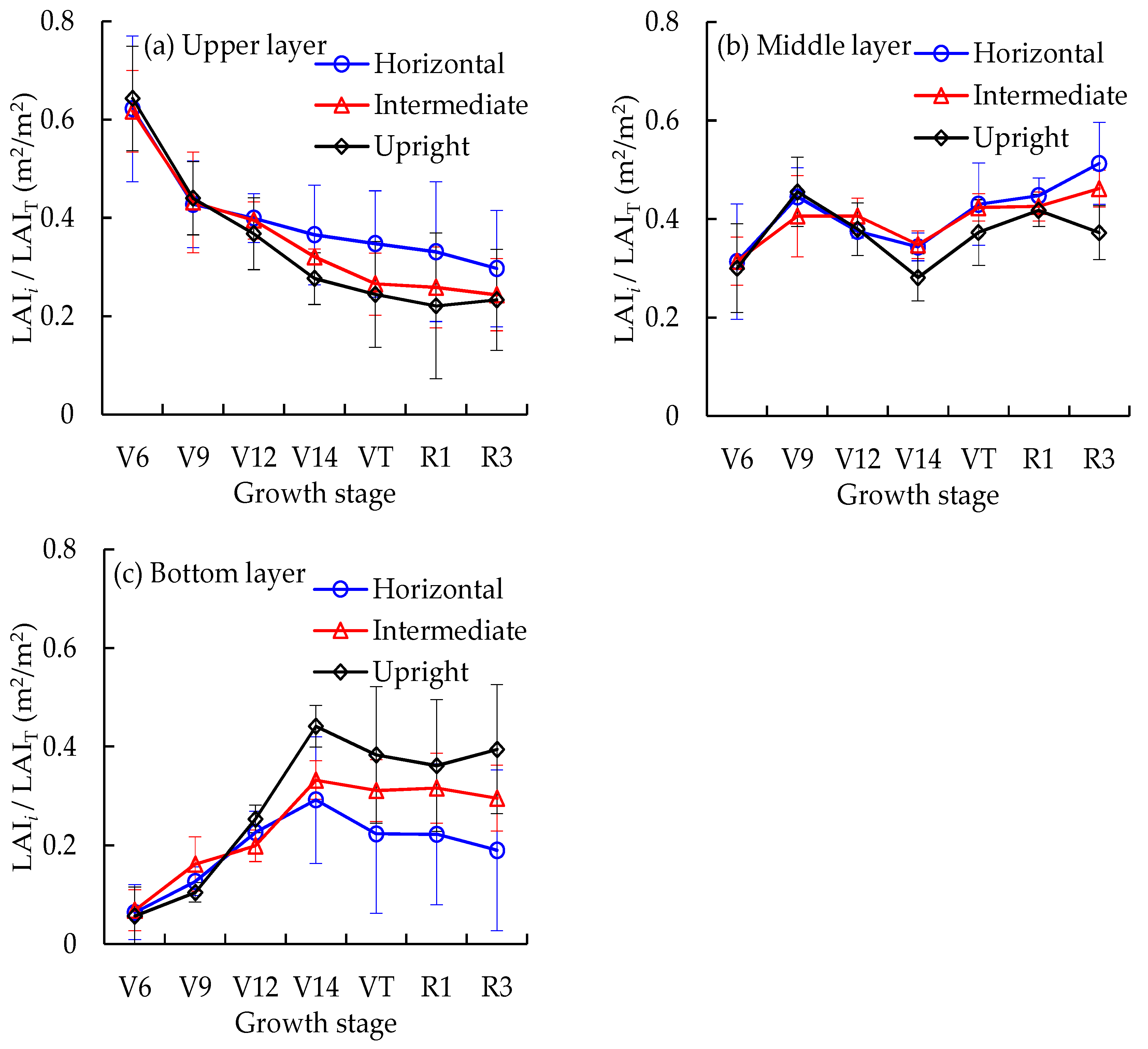
3.1. Canopy Structure Characteristics

As shown in Figure 1, the upper layer LAI1/LAIT of the horizontal, intermediate, and upright leaf varieties ranged from 0.30 to 0.62, 0.24 to 0.62, and 0.22 to 0.64, respectively, decreasing with maize growth. Prior to the V12 stage, there were small differences in the LAI1/LAIT among the different plant geometry types, whereas, after the V12 stage, the LAI1/LAIT of the upright varieties decreased the most, followed by the intermediate varieties and horizontal varieties. In contrast, the LAI3/LAIT of the bottom layer of all plant types initially increased prior to the V14 stage and after that, it decreased slightly as the crop grew. The LAI3/LAIT ranged from 0.06 to 0.29 for the horizontal varieties, from 0.07 to 0.33 for the intermediate varieties, and from 0.06 to 0.44 for the upright varieties. The LAI2/LAIT values of the middle layer of the three plant types were relatively stable during the entire growth period.
Furthermore, the differences in the LAIi/LAIT among the different varieties became more apparent after the V14 stage. The coefficients of variation (CV) of the LAI1/LAIT of the different plant types after the V14 stage ranged from 13.3 to 20.7% with a mean of 16.7%, whereas it varied from 1.4 to 4.4% with a relatively small mean of 2.7% prior to the V12 stage. Similar to the upper layer, the variation of the LAI3/LAIT of the different plant types was greater after the V14 stage (CV ranged from 21.8 to 35.0% with a mean of 26.7%) than before the V12 stage (CV ranged from 9.3 to 22.1% with a mean of 14.4%). The difference in the LAI2/LAIT between the different plant types was relatively small.

3.2. Vertical Distribution Characteristics of Leaf N Density

The LND values of the vertical canopy layers of the different plant geometry types are listed in Table 2. From top to bottom within the canopies, the LND showed a decreasing trend. For the horizontal leaf varieties across the growth stages, the LND at the bottom layer ranged between 0.13 and 2.66 g m−2 (mean = 0.93 g m−2, and CV = 80.0%) and was lower but more variable than that in the upper and middle layers, where the LND was from 1.30 to 3.71 g m−2 (mean = 2.22 g m−2, and CV = 28.0%) and 0.50 to 2.91 g m−2 (mean = 1.82 g m−2, and CV = 29.1%), respectively. This trend was also true for both the intermediate and upright leaf varieties. The variation in LND was larger in the bottom layer than that in the upper and middle layers across all the stages, and the CV values in the upper, middle and bottom layers of the intermediate leaf varieties were 27.8%, 33.2% and 68.3%, respectively, and for the upright leaf varieties, the values were 25.3%, 34.8% and 81.4%, respectively. The average LND values in the bottom layer of the intermediate and upright leaf varieties were 1.08 and 1.18 g m−2, respectively, and both were significantly lower than those in the upper and middle layers. This is consistent with previous studies, which reported that the lower shaded leaves generally have a lower N content than the upper illuminated leaves [21,28,29,63,64]. The LND gradient between the upper and bottom layers was 1.29 g m−2 for the horizontal varieties, 1.09 g m−2 for the intermediate varieties, and 0.85 g m−2 for the upright varieties, respectively, indicating that the vertical N gradients decreased as the canopy leaves changed to a more upright geometry. This occurs because the upright leaf variety has a high light transmittance rate, and leaves growing under better light conditions accumulate more N than shaded leaves [31]. In addition, the average LND values in the bottom layer were lower during the V6 to V12 stages than during the V14 to R3 stages (0.57 vs. 1.18 g m−2 for the horizontal varieties, 0.65 vs. 1.14 g m−2 for the intermediate varieties, and 0.64 vs. 1.56 g m−2 for the upright varieties, respectively).

3.3. Performance of Published Vegetation Indices

The correlation analysis results between the published indices and the LND in the vertical canopy layers of the different plant geometry types are shown in Table 3. All 12 published indices performed well for the upper layer (p < 0.05) for all varieties and growth stages. As the depth of the canopy increased, the correlations between the LND and the published indices gradually weakened, but they differed among the plant types. For the bottom layer of the canopy, the five best performing published indices for the upright leaf varieties were SR 1, SR 2, normalized differentiated red-edge index (NDRE), MERIS terrestrial chlorophyll index (MTCI), and double-peak nitrogen index (NDDA) with R2 values ranging from 0.42 to 0.48, whereas those for intermediate leaf varieties were SR 1, SR 2, green-normalized differentiated vegetation index (NDVI), NDRE, and modified chlorophyll absorption ratio index (MCARI) with R2 values ranging from 0.18 to 0.20. The horizontal leaf varieties had low correlations between the bottom layer LND and the spectral indices (R2 < 0.02, p > 0.05).
For the different growth stages, the correlation between the upper-layer LND and the published indices was higher before the V12 stage than after the V12 stage. The possible reason is that the spectral information of the upper leaves is influenced by the maize tassels at the top of the canopy during the later stages. Similar to the results for the upper layer, the bottom-layer LND of all varieties had good correlations with the published indices during the V6 to V12 stages. In comparison, during the V14 to R3 stages, the correlations varied greatly for the different varieties during the V14 to R3 stages. The upright leaf varieties exhibited the best correlations between the LND and all the published indices and were significant at the 0.05 significance level (R2 ranging from 0.20 to 0.39). The intermediate leaf varieties exhibited significant correlations at the 0.05 significance level (R2 ranging from 0.15–0.22), whereas the horizontal leaf varieties had non-significant correlations with the published indices (R2 < 0.17, p > 0.05).

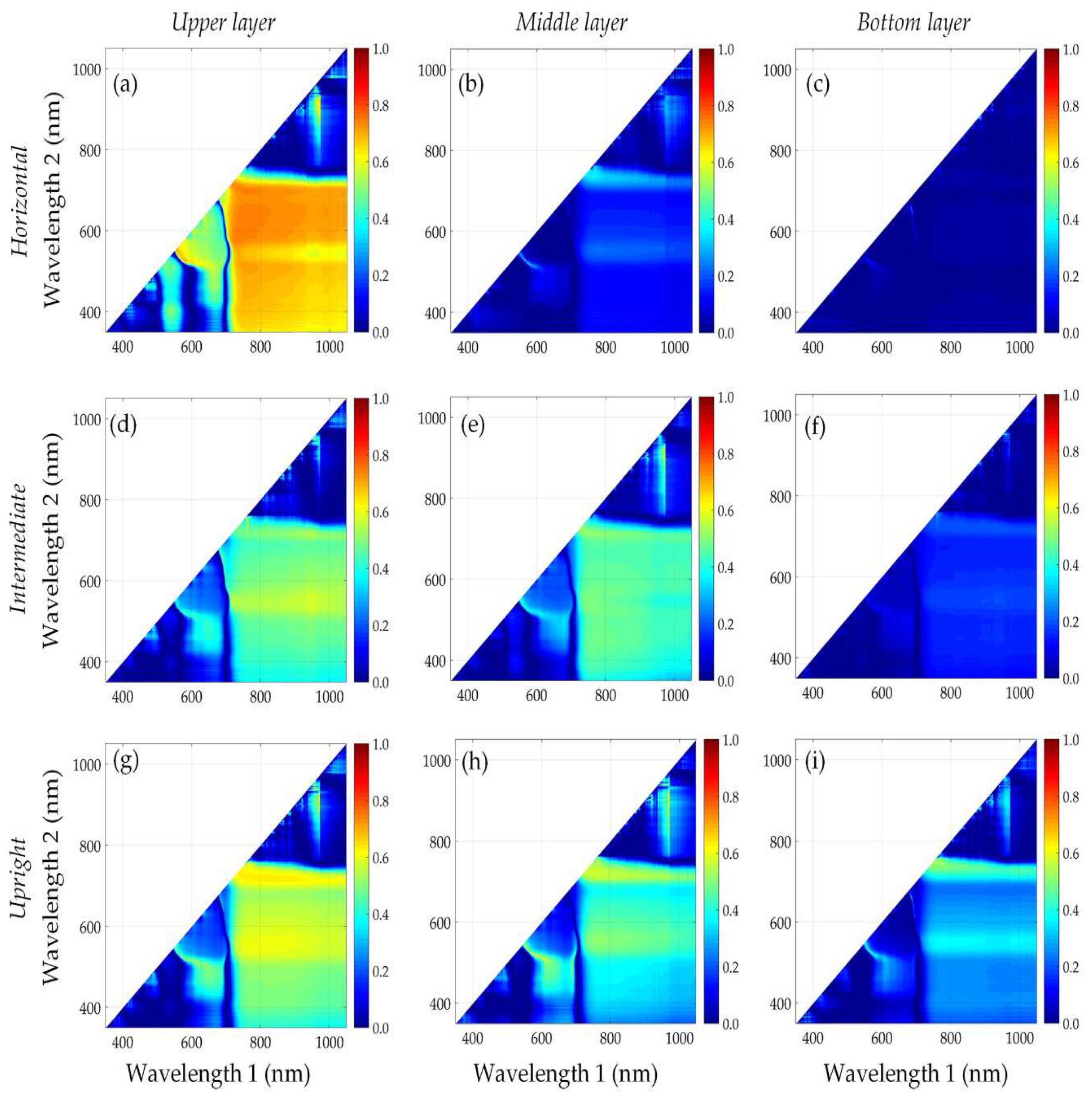
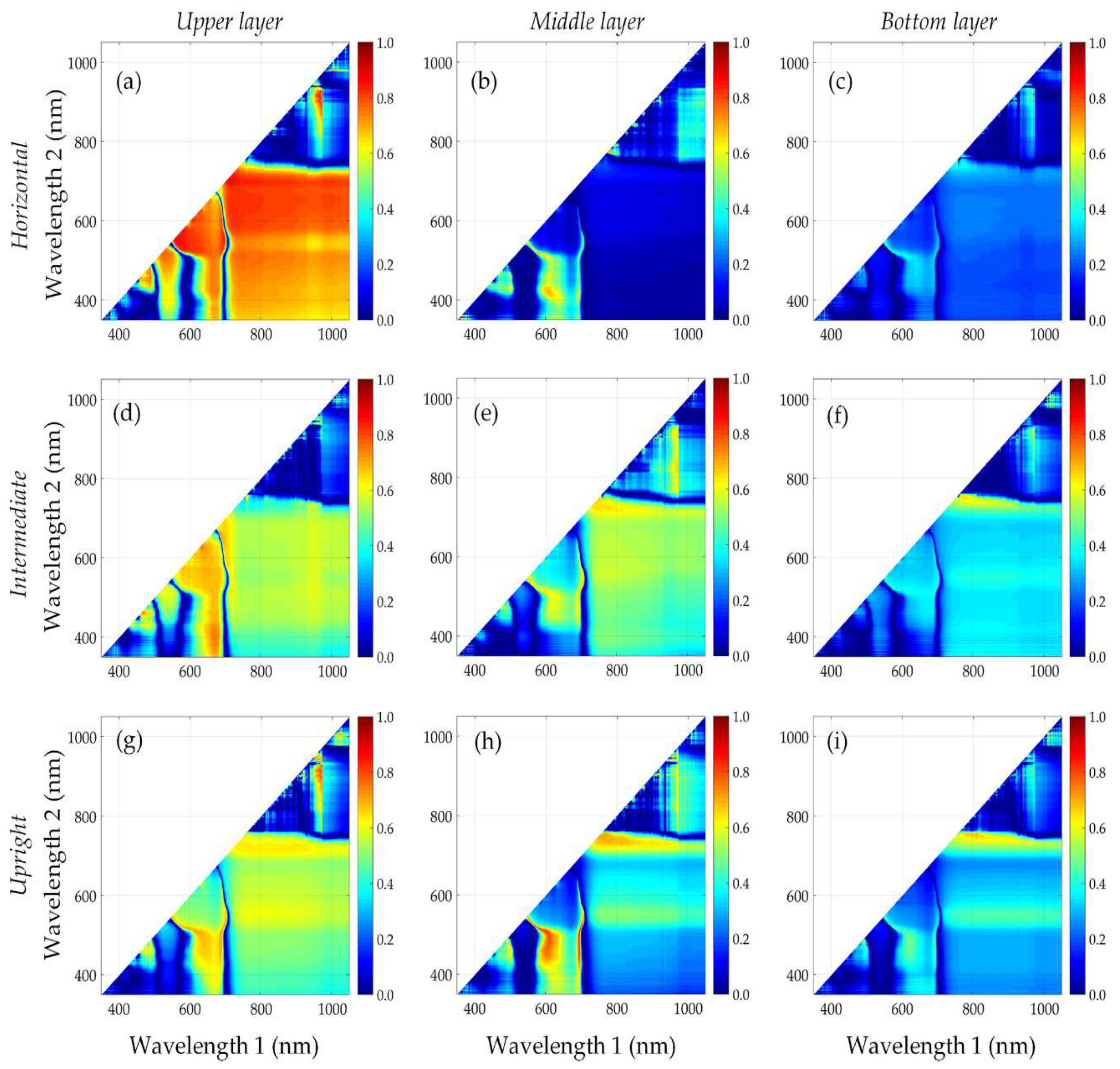
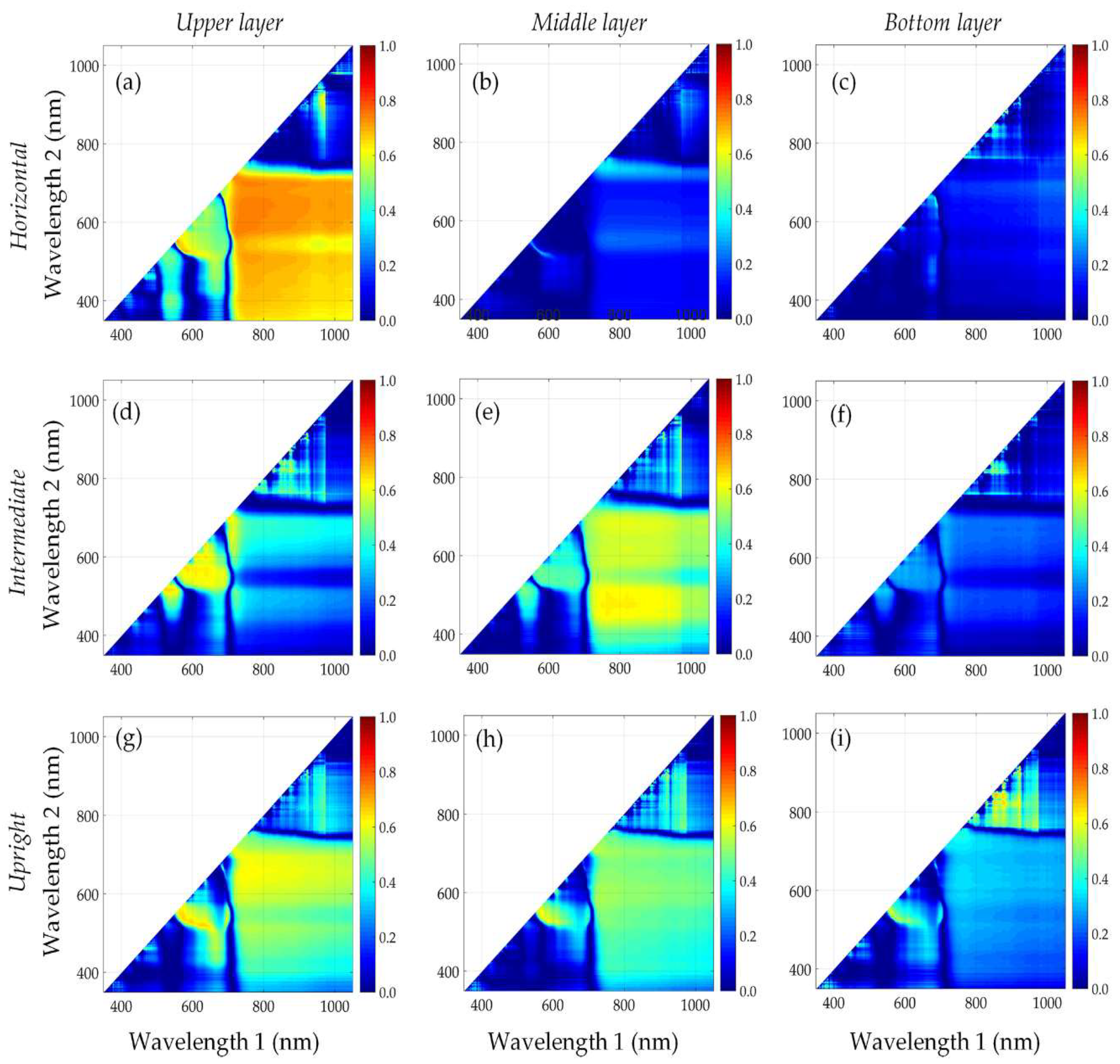
3.4. Identification of New Vegetation Indices

The analysis of the published VIs shows that the SR index generally provided a good estimate of the LND vertical distribution in the maize canopy. Therefore, we further examined all the possible 2-band combinations from 350 to 1150 nm and correlated them with the LND in the different canopy layers. The matrix plots of the coefficients of determination (R2) between the SRs and the LND show that the relationships varied in terms of canopy layers, plant geometry types, and growth stages (Figure 2, Figure 3 and Figure 4). Consistent with the results of the published vegetation indices, the R2 for the SRs was higher for the upper layer than the lower layers. The R2 values of the lower layers exhibited greater differences in the contour plots for the different maize plant geometry types (Figure 2). When the data for all growth stages were combined, the performances of the SRs were significantly affected by the plant geometry types, especially in the middle and the bottom layers. For instance, in the bottom layers of both the intermediate and upright leaf varieties, the highest R2 values were observed for the red-edge bands (700–760 nm) paired with the red-edge to near-infrared (NIR) bands (700–1050 nm), followed by the green bands (550–580 nm) paired with the red-edge to NIR bands (700–1050 nm). The best new SR index (736, 812) produced the highest R2 value of 0.52 for all stages for modeling the bottom-layer LND of the upright leaf varieties. The same SR index (736, 812) was also suitable for estimating the upper and middle-layer LND of the upright leaf varieties, with R2 values of 0.50 and 0.60, respectively. For the intermediate leaf varieties, the highest R2 value generated by the SR index (721, 935) was only 0.25. For the horizontal leaf varieties, however, few bands showed sensitivity to the bottom-layer LND.
For the different growth stages, there were good correlations between the SRs and the LND for all canopy layers except for the horizontal leaf varieties during the V6 to V12 stages. The sensitive bands in the middle and bottom layers were centered at (i) the red-edge bands (700–760 nm) paired with the red-edge to NIR bands (700–1050 nm) and (ii) the blue bands (440–490 nm) paired with the orange bands (590–640 nm) (Figure 3). For the bottom layer, for example, the best new SRs yielded large R2 values than the published indices. The R2 values were 0.71 for the SR index (753, 812), 0.63 for the SR index (748, 793), and 0.38 for the SR index (740, 775) for the upright, intermediate, and horizontal leaf varieties, respectively. In comparison, during the V14 to R3 stages, the R2 values for the SRs were considerably lower for the bottom layer. The sensitive bands for the bottom layer were shifted to (i) the orange to red bands (590–710 nm) paired with the red-edge to NIR bands (710–1050 nm) and (ii) green bands (520–600 nm) paired with the red bands (600–700 nm) (Figure 4). The SR index (524, 583) and SR index (591, 611) were the best new SRs for the upright (R2 = 0.54) and intermediate (R2 = 0.30) leaf varieties, respectively. Additionally, there were also very poor relationships between the SRs and the bottom-layer LND of the horizontal leaf varieties.

4. Discussion

The non-uniformity of the vertical leaf N distribution in the canopy of plants has been demonstrated in many studies; i.e., the lower shaded leaves generally have a lower N content than the upper illuminated leaves [21,28,29,63,64]. Our results revealed that there were significant differences in the LAIi/LAIT between the different maize plant geometry types (i.e., the order of the upper-layer LAI1/LAIT was horizontal leaf varieties > intermediate leaf varieties > upright leaf varieties, whereas the order of the bottom-layer LAI3/LAIT was upright leaf varieties > horizontal leaf varieties > intermediate leaf varieties). This resulted in a decrease in the vertical N gradients between the upper layer and the bottom layer as the plant type changed to a more upright geometry (i.e., 1.29, 1.09, and 0.85 g m−2 for the horizontal, intermediate, and upright varieties, respectively). In addition, the variation in the bottom-layer LND was larger than that of the upper-layer LND across the entire growth period (i.e., CV: 80.0% vs. 28.0% for the horizontal leaf varieties, 68.3% vs. 33.2% for the intermediate leaf varieties, 81.4% vs. 34.8% for the upright leaf varieties). This is consistent with the results of Lu (1994) [22], who reported that the lower leaves of the crop canopy are more sensitive to N deficiency or N translocation than the upper leaves.
The most encouraging result, however, was that the maize geometry plant type had a significant effect on the detectability of the vertical leaf N distribution in the canopy using canopy spectral reflectance, as well as the sensitivity of the bands. As shown in Table 2 and Figure 3, the correlations are higher between the lower leaf N and the spectral indices (both for the published indices and the new SRs) for maize plants with upright leaves than those with relatively flat leaves. For the bottom layers of the upright leaf varieties, the red edge and NIR bands performed better than the visible bands, which is in agreement with the results of Feng et al. (2008) [65] for wheat and those of Yu et al. (2013) [14] for rice. Actually, 52% of the variation in the bottom layer LND of upright leaf varieties was explained by the best performing newly proposed SR index (736, 812), whereas only 25% of the variation in the bottom layer LND of the intermediate leaf varieties was explained by the best performing newly proposed SR index (721, 935). Few bands were sensitive to the LND of the bottom layer of the horizontal leaf varieties. This is attributed to the fact that, in plants with upright leaves, the bottom layer contributes more to the canopy spectral reflectance than in plants with relatively flat leaves [30,32,33,34,37].
The results also showed that the growth stages had a large influence on the remote estimation of the N vertical distribution in the canopy. During the V6 to V12 stages, the sensitive bands for detecting the bottom leaf N were the red-edge bands (700–760 nm) paired with the red-edge to NIR bands (700–1050 nm), and these were shifted to the orange to red bands (590–710 nm) paired with the red-edge to NIR bands (710–1050 nm) during the V14 to R3 stages. This occurred because the canopy reflectance was dominated by the biomass before the V12 stage and by the plant N after this stage [14]. In addition, many studies have shown that the green duration and the senescence speed of the lower leaves of the crop are closely related to the amount of light quanta that is received [34,66]. When the canopy is fully closed during the later growth stage (i.e., after the V14 stage in this study), the bottom leaves begin to senesce and wilt.
The timely and accurate diagnosis of maize N nutritional status is essential for precise N management. The vertical leaf N distribution is very important for N status diagnosis because when N is deficient, lower leaves will show deficiency symptoms first. The results of this study indicated that it was feasible to estimate the N vertical distribution in the maize canopy using canopy hyperspectral reflectance before the V12 stage. These results provide a theoretical basis for early diagnosis of maize N status using remote sensing for precision N management, especially for upright leaf type varieties. According to the local standard practices, the topdressing of N for maize is mainly applied between V6 and V12 stages. The N vertical distribution information in the canopy of maize before the V12 stage can be used to guide in-season N management. More studies are needed to develop corresponding N recommendation algorithms based on such information. However, there are still some limitations in this study. The factors affecting the reflectivity should be considered in future research; for example, the sun angle, background, LAI, leaf angle distribution, and pigment content [67,68]. Moreover, the hyperspectral reflectance data obtained from the top of the canopy by ASD FieldSpec® Pro FR spectroradiometer represents spectrally mixed information because the upper, middle, and bottom-layer leaves cannot be distinguished. In the future, we plan to use hyperspectral imaging acquired from different zenith and azimuth angles, which may be more suitable for estimating the vertical N distribution in the crop canopy. A fusion of LiDAR and hyperspectral (or multispectral) data collected from unmanned aerial vehicle (UAV) platforms also has great potential in estimating N vertical distribution in the crop canopies at field and farm scales for precision agriculture applications.

5. Conclusions

This study evaluated the influences of the maize plant geometry (i.e., horizontal type, intermediate type, and upright type) on the remote estimation of the vertical N distribution in a canopy at different growth stages. The results showed that there were significant differences between the three maize plant geometry types in terms of canopy architecture and N vertical distribution. The vertical LND gradients between the upper layer and bottom layer decreased as the leaves of the maize changed to a more upright geometry (i.e., 1.29, 1.09, and 0.85 g m−2 for the horizontal, intermediate, and upright varieties, respectively). In comparison, the lower-layer LND was more sensitive than the upper-layer LND for the combined growth stages. The results also showed that the maize plant geometry had a significant impact on the estimation of the vertical N distribution based on canopy spectral reflectance. The upright leaf varieties had the highest correlation between the lower-layer LND (R2 = 0.52) and the new SR index (736, 812), and this index also performed well for estimating the upper (R2 = 0.50) and middle (R2 = 0.60) layer LND. However, for the intermediate leaf variety, only 25% of the variation in the bottom-layer LND was explained by the best new SR index (721, 935) and few bands showed sensitivity to the bottom-layer LND of the horizontal leaf varieties. Furthermore, the growth stages also influenced the remote detection of the lower-leaf N status of the canopy, because the canopy reflectance was dominated by the biomass before the V12 stage and by the plant N after this stage. Therefore, we can conclude that a more accurate estimation of the N vertical distribution in the canopy can be obtained by canopy hyperspectral reflectance for maize plants with more upright leaves.

Author Contributions

H.Y. performed the data analysis and wrote the manuscript. W.H. conducted the field experiments and guided the study. S.H., B.W., Y.D. and B.C. provided suggestions for the study, reviewed and edited the manuscript. All authors read and approved the manuscript.

Funding

This research was funded by the National Natural Science Foundation of China (41871339, 41501468, 41571354, 41601466), the Key Laboratory of Agricultural Big Data, Ministry of Agriculture and Rural Affairs, Beijing, China, and Hainan Provincial Department of Science and Technology under Grant (ZDKJ2016021, ZDKJ2017009).

Acknowledgments

We would like to thank the field campaign at the National Experimental Station for Precision Agriculture, Beijing, China.

Conflicts of Interest

The authors declare no conflict of interest.

References

  1. Sheehy, J.E.; Dionora, M.J.A.; Mitchell, P.L.; Peng, S.; Cassman, K.G.; Lemaire, G.; Williams, R.L. Critical nitrogen concentrations: Implications for high-yielding rice (Oryza sativa L.) cultivars in the tropics. Field Crop Res. 1998, 59, 31–41. [Google Scholar] [CrossRef]
  2. Ziadi, N.; Bélanger, G.; Claessens, A.; Lefebvre, L.; Cambouris, A.N.; Tremblay, N.; Nolin, M.C.; Parent, L.É. Determination of a critical nitrogen dilution curve for spring wheat. Agron. J. 2010, 102, 241–250. [Google Scholar] [CrossRef]
  3. Yue, S.C.; Sun, F.L.; Meng, Q.F.; Zhao, R.F.; Li, F.; Chen, X.P.; Zhang, F.S.; Cui, Z.L. Validation of a critical nitrogen curve for summer maize in the North China Plain. Pedosphere 2014, 24, 76–83. [Google Scholar] [CrossRef]
  4. Scholberg, J.; McNeal, B.L.; Boote, K.J.; Jones, J.W.; Locascio, S.J.; Olson, S.M. Nitrogen stress effects on growth and nitrogen accumulation by field-grown tomato. Agron. J. 2000, 92, 159–167. [Google Scholar] [CrossRef]
  5. Zhao, D.; Reddy, K.R.; Kakani, V.G.; Reddy, V.R. Nitrogen deficiency effects on plant growth, leaf photosynthesis, and hyperspectral reflectance properties of sorghum. Eur. J. Agron. 2005, 22, 391–403. [Google Scholar] [CrossRef]
  6. Boussadia, O.; Steppe, K.; Zgallai, H.; El Hadj, S.B.; Braham, M.; Lemeur, R.; Van Labeke, M.C. Effects of nitrogen deficiency on leaf photosynthesis, carbohydrate status and biomass production in two olive cultivars ‘Meski’and ‘Koroneiki’. Sci. Hortic. 2010, 123, 336–342. [Google Scholar] [CrossRef]
  7. Zhang, Y.; Tan, L.; Zhu, Z.; Yuan, L.; Xie, D.; Sun, C. TOND1 confers tolerance to nitrogen deficiency in rice. Plant J. 2015, 81, 367–376. [Google Scholar] [CrossRef] [Green Version]
  8. Ju, X.T.; Xing, G.X.; Chen, X.P.; Zhang, S.L.; Zhang, L.J.; Liu, X.J.; Cui, Z.L.; Yin, B.; Christie, P.; Zhu, Z.L.; et al. Reducing environmental risk by improving N management in intensive Chinese agricultural systems. Proc. Natl. Acad. Sci. USA 2009, 106, 3041–3046. [Google Scholar] [CrossRef] [Green Version]
  9. Huang, W.; Yang, Q.; Pu, R.; Yang, S. Estimation of Nitrogen Vertical Distribution by Bi-Directional Canopy Reflectance in Winter Wheat. Sensors 2014, 14, 20347–20359. [Google Scholar] [CrossRef] [Green Version]
  10. Qiu, S.J.; He, P.; Zhao, S.C.; Li, W.J.; Xie, J.G.; Hou, Y.P.; Grant, C.A.; Zhou, W.; Jin, J.Y. Impact of Nitrogen Rate on Maize Yield and Nitrogen Use Efficiencies in Northeast China. Agron. J. 2015, 107, 305–313. [Google Scholar] [CrossRef]
  11. Li, F.; Miao, Y.; Hennig, S.D.; Gnyp, M.L.; Chen, X.; Jia, L.; Bareth, G. Evaluating hyperspectral vegetation indices for estimating nitrogen concentration of winter wheat at different growth stages. Precis. Agric. 2010, 11, 335–357. [Google Scholar] [CrossRef]
  12. Hansen, P.M.; Schjoerring, J.K. Reflectance measurement of canopy biomass and nitrogen status in wheat crops using normalized difference vegetation indices and partial least square regression. Remote Sens. Environ. 2003, 86, 542–553. [Google Scholar] [CrossRef]
  13. Xue, L.; Cao, W.; Luo, W.; Dai, T.; Zhu, Y. Monitoring leaf nitrogen status in rice with canopy spectral reflectance. Agron. J. 2004, 96, 135–142. [Google Scholar] [CrossRef]
  14. Yu, K.; Li, F.; Gnyp, M.L.; Miao, Y.; Bareth, G.; Chen, X. Remotely detecting canopy nitrogen concentration and uptake of paddy rice in the Northeast China Plain. ISPRS-J. Photogramm. Remote Sens. 2013, 78, 102–115. [Google Scholar] [CrossRef]
  15. Huang, S.; Miao, Y.; Zhao, G.; Yuan, F.; Ma, X.; Tan, C.; Yu, W.; Gnyp, M.L.; Lenz-Wiedemann, V.I.S.; Rascher, U.; et al. Satellite remote sensing-based in-season diagnosis of rice nitrogen status in Northeast China. Remote Sens. 2015, 7, 10646–10667. [Google Scholar] [CrossRef]
  16. He, L.; Song, X.; Feng, W.; Guo, B.B.; Zhang, Y.S.; Wang, Y.H.; Wang, C.Y.; Guo, T.C. Improved remote sensing of leaf nitrogen concentration in winter wheat using multi-angular hyperspectral data. Remote Sens. Environ. 2016, 174, 122–133. [Google Scholar] [CrossRef]
  17. Dreccer, M.F.; Slafer, G.A.; Rabbinge, R. Optimization of vertical distribution of canopy nitrogen. J. Crop Prod. 1997, 1, 47–77. [Google Scholar] [CrossRef]
  18. Dreccer, M.F.; Van Oijen, M.; Schapendonk, A.H.C.M.; Pot, C.S.; Rabbinge, R. Dynamics of vertical leaf nitrogen distribution in a vegetative wheat canopy. Impact on canopy photosynthesis. Ann. Bot. 2000, 86, 821–831. [Google Scholar] [CrossRef]
  19. Huang, W.; Wang, Z.; Huang, L.; Lamb, D.W.; Ma, Z.; Zhang, J.; Wang, J.; Zhao, C. Estimation of vertical distribution of chlorophyll concentration by bi-directional canopy reflectance spectra in winter wheat. Precis. Agric. 2011, 12, 165–178. [Google Scholar] [CrossRef]
  20. Wang, Z.; Wang, J.; Zhao, C.; Zhao, M.; Huang, W.; Wang, C. Vertical distribution of nitrogen in different layers of leaf and stem and their relationship with grain quality of winter wheat. J. Plant Nutr. 2012, 28, 73–91. [Google Scholar] [CrossRef]
  21. Li, H.; Zhao, C.; Huang, W.; Yang, G. Non-uniform vertical nitrogen distribution within plant canopy and its estimation by remote sensing: A review. Field Crop Res. 2013, 142, 75–84. [Google Scholar] [CrossRef]
  22. Lu, J.L. Plant Nutrition, 1st ed.; the First Volume; Beijing Agricultural University Press (continuing China Agricultural University Press): Beijing, China, 1994. (In Chinese) [Google Scholar]
  23. Wang, Z.; Wang, J.; Liu, L.; Huang, W.; Zhao, C.; Lu, Y. Estimation of nitrogen status in middle and bottom layers of winter wheat canopy by using ground-measured canopy reflectance. Commun. Soil Sci. Plant 2005, 36, 2289–2302. [Google Scholar] [CrossRef]
  24. Wang, J.H.; Huang, W.J.; Lao, C.L.; Zhang, L.D.; Luo, C.B.; Wang, T.; Liu, L.Y.; Song, X.Y.; Ma, Z.H. Inversion of winter wheat foliage vertical distribution based on canopy reflected spectrum by partial least squares regression method. Spectrosc. Spect. Anal. 2007, 27, 1319–1322, (In Chinese with English abstract). [Google Scholar]
  25. Ciganda, V.S.; Gitelson, A.A.; Schepers, J. How deep does a remote sensor sense? expression of chlorophyll content in a maize canopy. Remote Sens. Environ. 2012, 126, 240–247. [Google Scholar] [CrossRef]
  26. Hirose, T.; Werger, M.J.A.; Pons, T.L.; van Rheenen, J.W.A. Canopy structure and leaf nitrogen distribution in a stand of Lysimachia vulgaris L. as influenced by stand density. Oecologia 1988, 77, 145–150. [Google Scholar] [CrossRef]
  27. Anten, N.P.R.; Schieving, F.; Werger, M.J.A. Patterns of light and nitrogen distribution in relation to whole canopy carbon gain in C3 and C4 mono- and dicotyledonous species. Oecologia 1995, 101, 504–513. [Google Scholar] [CrossRef] [PubMed]
  28. Lötscher, M.; Stroh, K.; Schnyder, H. Vertical leaf nitrogen distribution in relation to nitrogen status in grassland plants. Ann. Bot. 2003, 92, 679–688. [Google Scholar] [CrossRef]
  29. Bertheloot, J.; Martre, P.; Andrieu, B. Dynamics of light and nitrogen distribution during grain filling within wheat canopy. Plant Physiol. 2008, 148, 1707–1720. [Google Scholar] [CrossRef]
  30. Monsi, M.; Saeki, T. On the factor light in plant communities and its importance for matter production. Ann. Bot. 2005, 95, 549–567. [Google Scholar] [CrossRef]
  31. Hirose, T.; Werger, M.J.A. Maximizing daily canopy photosynthesis with respect to the leaf nitrogen allocation pattern in the canopy. Oecologia 1987, 72, 520–526. [Google Scholar] [CrossRef]
  32. Maddonni, G.A.; Otegui, M.E.; Cirilo, A.G. Plant population density, row spacing and hybrid effects on maize canopy architecture and light attenuation. Field Crop. Res. 2001, 71, 183–193. [Google Scholar] [CrossRef]
  33. Lambert, R.J.; Johnson, R.R. Leaf angle, tassel morphology, and the performance of maize hybrids. Crop Sci. 1978, 18, 499–502. [Google Scholar] [CrossRef]
  34. Azumi, Y.; Watanabe, A. Evidence for a senescence-associated gene induced by darkness. Plant Physiol. 1991, 95, 577–583. [Google Scholar] [CrossRef] [PubMed]
  35. Ku, L.X.; Zhao, W.M.; Zhang, J.; Wu, L.C.; Wang, C.L.; Wang, P.A.; Zhang, W.Q.; Chen, Y.H. Quantitative trait loci mapping of leaf angle and leaf orientation value in maize (Zea mays L.). Theor. Appl. Genet. 2010, 121, 951–959. [Google Scholar] [CrossRef] [PubMed]
  36. Duvick, D.N.; Smith, J.S.C.; Cooper, M. Long-term selection in a commercial hybrid maize breeding program. Plant Breed. Rev. 2004, 24, 109–151. [Google Scholar]
  37. Ma, D.L.; Xie, R.Z.; Niu, X.K.; Li, S.K.; Long, H.L.; Liu, Y.E. Changes in the morphological traits of maize genotypes in China between the 1950s and 2000s. Eur. J. Agron. 2014, 58, 1–10. [Google Scholar] [CrossRef]
  38. Tong, P. The course and the achievement of corn variety improvement in the20th century in China. China Hist. Mater. Sci. Technol. 2001, 22, 113–127. [Google Scholar]
  39. Meghji, M.R.; Dudley, J.W.; Lambert, R.J.; Sprague, G.F. Inbreeding depression, inbred and hybrid grain yields, and other traits of maize genotypes representing three eras. Crop Sci. 1984, 24, 545–549. [Google Scholar] [CrossRef]
  40. Russell, W.A. Genetic improvement of maize yields. Adv. Agron. 1991, 46, 245–298. [Google Scholar]
  41. IUSS Working Group WRB. World Reference Base for Soil Resources 2006; World Soil Resources Reports No. 103; FAO: Rome, Italy, 2006. [Google Scholar]
  42. Soil Survey Division Staff. Soil Survey Manual; United States Department of Agriculture: Washington, DC, USA, 1993.
  43. Pepper, G.E.; Pearce, R.B.; Mock, J.J. Leaf orientation and yield of maize. Crop Sci. 1977, 17, 883–886. [Google Scholar] [CrossRef]
  44. Jonckheere, I.; Fleck, S.; Nackaerts, K.; Muys, B.; Coppin, P.; Weiss, M.; Baret, F. Methods for leaf area index determination. Part I: Theories, techniques and instruments. Agric. For. Meteorol. 2004, 121, 19–35. [Google Scholar] [CrossRef]
  45. Helrich, K. Official Methods of Analysis of the AOAC, 15th ed.; AOAC: Arlington, VA, USA, 1990; pp. 16–17. [Google Scholar]
  46. Greenwood, D.J.; Neeteson, J.J.; Draycott, A. Quantitative relationships for the dependence of growth rate of arable crops on their nitrogen content, dry weight and aerial environment. In Fundamental, Ecological and Agricultural Aspects of Nitrogen Metabolism in Higher Plants; Springer: Dordrecht, The Netherlands, 1986; Volume 91, pp. 281–301. [Google Scholar]
  47. Giletto, C.M.; Echeverría, H.E. Critical nitrogen dilution curve for processing potato in Argentinean humid pampas. Am. J. Potato Res. 2012, 89, 102–110. [Google Scholar] [CrossRef]
  48. Mistele, B.; Schmidhalter, U. Estimating the nitrogen nutrition index using spectral canopy reflectance measurements. Eur. J. Agron. 2008, 29, 184–190. [Google Scholar] [CrossRef]
  49. Hirose, T.; Werger, M.J.A.; van Rheenen, J.W.A. Canopy development and leaf nitrogen distribution in a stand of Carex acutiformis. Ecology 1989, 70, 1610–1618. [Google Scholar] [CrossRef]
  50. Archontoulis, S.V.; Vos, J.; Yin, X.; Bastiaans, L.; Danalatos, N.G.; Struik, P.C. Temporal dynamics of light and nitrogen vertical distributions in canopies of sunflower, kenaf and cynara. Field Crop Res. 2011, 122, 186–198. [Google Scholar] [CrossRef]
  51. Schieving, F.; Pons, T.L.; Werger, M.J.A.; Hirose, T. The vertical distribution of nitrogen and photosynthetic activity at different plant densities in Carex acutiformis. Plant Soil 1992, 14, 9–17. [Google Scholar] [CrossRef]
  52. Zarco-Tejada, P.J.; Miller, J.R.; Noland, T.L.; Mohammed, G.H.; Sampson, P.H. Scaling-up and model inversion methods with narrowband optical indices for chlorophyll content estimation in closed forest canopies with hyperspectral data. IEEE Trans. Geosci. Remote Sens. 2001, 39, 1491–1507. [Google Scholar] [CrossRef] [Green Version]
  53. Blackburn, G.A. Quantifying chlorophylls and carotenoids at leaf and canopy scales: An evaluation of some hyperspectral approaches. Remote Sens. Environ. 1998, 66, 273–285. [Google Scholar] [CrossRef]
  54. Gitelson, A.; Merzlyak, M.N. Quantitative estimation of chlorophyll-a using reflectance spectra: Experiments with autumn chestnut and maple leaves. J. Photochem. Photobiol. B-Biol. 1994, 22, 247–252. [Google Scholar] [CrossRef]
  55. Fitzgerald, G.J.; Rodriguez, D.; Christensen, L.K.; Belford, K.; Sadras, V.O.; Clarke, T.R. Spectral and thermal sensing for nitrogen and water status in rainfed and irrigated wheat environments. Precis. Agric. 2006, 7, 233–248. [Google Scholar] [CrossRef]
  56. Rondeaux, G.; Steven, M.; Baret, F. Optimization of soil-adjusted vegetation indices. Remote Sens. Environ. 1996, 55, 95–107. [Google Scholar] [CrossRef]
  57. Dash, J.; Curran, P.J. The MERIS terrestrial chlorophyll index. Int. J. Remote Sens. 2004, 25, 5403–5413. [Google Scholar] [CrossRef]
  58. Feng, W.; Guo, B.B.; Wang, Z.J.; He, L.; Song, X.; Wang, Y.H.; Guo, T.C. Measuring leaf nitrogen concentration in winter wheat using double-peak spectral reflection remote sensing data. Field Crop. Res. 2014, 159, 43–52. [Google Scholar] [CrossRef]
  59. Sims, D.A.; Gamon, J.A. Relationships between leaf pigment content and spectral reflectance across a wide range of species, leaf structures and developmental stages. Remote Sens. Environ. 2002, 81, 331–354. [Google Scholar] [CrossRef]
  60. Le Maire, G.; François, C.; Soudani, K.; Berveiller, D.; Pontailler, J.Y.; Bréda, N.; Genet, H.; Davi, H.; Dufrêne, E. Calibration and validation of hyperspectral indices for the estimation of broadleaved forest leaf chlorophyll content, leafmass per area, leaf area index and leaf canopy biomass. Remote Sens. Environ. 2008, 112, 3846–3864. [Google Scholar] [CrossRef]
  61. Wu, C.; Niu, Z.; Tang, Q.; Huang, W. Estimating chlorophyll content from hyperspectral vegetation indices: Modeling and validation. Agric. For. Meteorol. 2008, 148, 1230–1241. [Google Scholar] [CrossRef]
  62. Daughtry, C.S.T.; Walthall, C.L.; Kim, M.S.; De Colstoun, E.B.; McMurtrey, J.E. Estimating corn leaf chlorophyll concentration from leaf and canopy reflectance. Remote Sens. Environ. 2000, 74, 229–239. [Google Scholar] [CrossRef]
  63. Drouet, J.L.; Bonhomme, R. Do variations in local leaf irradiance explain changes to leaf nitrogen within row maize canopies? Ann. Bot. 1999, 84, 61–69. [Google Scholar] [CrossRef]
  64. Shiratsuchi, H.; Yamagishi, T.; Ishii, R. Leaf nitrogen distribution to maximize the canopy photosynthesis in rice. Field Crop Res. 2006, 95, 291–304. [Google Scholar] [CrossRef]
  65. Feng, W.; Yao, X.; Zhu, Y.; Tian, Y.C.; Cao, W.X. Monitoring leaf nitrogen status with hyperspectral reflectance in wheat. Eur. J. Agron. 2008, 28, 394–404. [Google Scholar] [CrossRef]
  66. Ottman, M.J.; Welch, L.F. Supplemental radiation effects on senescence, plant nutrients, and yield of field-grown corn. Agron. J. 1988, 80, 619–626. [Google Scholar] [CrossRef]
  67. Schlemmer, M.; Gitelson, A.; Schepers, J.; Ferguson, R.; Peng, Y.; Shanahan, J.; Rundquistb, D. Remote estimation of nitrogen and chlorophyll contents in maize at leaf and canopy levels. Int. J. Appl. Earth Obs. Geoinf. 2013, 25, 47–54. [Google Scholar] [CrossRef] [Green Version]
  68. Feng, W.; Qi, S.; Heng, Y.; Zhou, Y.; Wu, Y.; Liu, W.; He, L.; Li, X. Canopy vegetation indices from in situ hyperspectral data to assess plant water status of winter wheat under powdery mildew stress. Front. Plant Sci. 2017, 8, 1219. [Google Scholar] [CrossRef] [PubMed]
Figure 1. Comparison of the relative leaf area index (LAI) (LAIi/LAIT) of the vertical canopy layers for different maize plant geometry types. LAIi/LAIT represents the ratio of the subtotal leaf area of a given layer (LAIi) to the total LAI of the canopy (LAIT). (a) Upper layer; (b) middle layer; (c) bottom layer. Error bars represent standard error of the mean.
Remotesensing 10 01995 g001
Figure 2. Maps showing the coefficients of determination (R2) for the relationships between the leaf N density and SR index calculated from all possible 2-band combinations in the range of 35–1050 nm across all stages. (a) The upper layer of horizontal leaf varieties; (b) the middle layer of the horizontal leaf varieties; (c) the bottom layer of the horizontal leaf varieties; (d) the upper layer of the intermediate leaf varieties; (e) the middle layer of the intermediate leaf varieties; (f) the bottom layer of the intermediate leaf varieties; (g) the upper layer of the upright leaf varieties; (h) the middle layer of the upright leaf varieties; and (i) the bottom layer of the upright leaf varieties.
Remotesensing 10 01995 g002
Figure 3. Maps showing the R2 for the relationships between the leaf N density and SR index calculated from all possible 2-band combinations in the range of 350–1050 nm during the V6 to V12 stages. (a) The upper layer of the horizontal leaf varieties; (b) the middle layer of the horizontal leaf varieties; (c) the bottom layer of the horizontal leaf varieties; (d) the upper layer of the intermediate leaf varieties; (e) the middle layer of the intermediate leaf varieties; (f) the bottom layer of the intermediate leaf varieties; (g) the upper layer of the upright leaf varieties; (h) the middle layer of the upright leaf varieties; and (i) the bottom layer of the upright leaf varieties.
Remotesensing 10 01995 g003
Figure 4. Maps showing the R2 for the relationships between the leaf N density and SR index calculated from all possible 2-band combinations in the range of 350–1050 nm during the V14 to R3 stages. (a) The upper layer of the horizontal leaf varieties; (b) the middle layer of the horizontal leaf varieties; (c) the bottom layer of the horizontal leaf varieties; (d) the upper layer of the intermediate leaf varieties; (e) the middle layer of the intermediate leaf varieties; (f) the bottom layer of the intermediate leaf varieties; (g) the upper layer of the upright leaf varieties; (h) the middle layer of the upright leaf varieties; and (i) the bottom layer of the upright leaf varieties.
Remotesensing 10 01995 g004
Table 1. Published vegetation indices used in this study.
IndexFormulaReference
Simple ratio (SR) 1B810/B560[13]
SR 2B750/B710[52]
Normalized difference vegetation index (NDVI)(B800 − B680)/(B800 + B680)[53]
Green NDVI(B750 − B550)/(B750 + B550)[54]
Normalized difference red edge (NDRE) Index(B790 − B720)/(B790 + B720)[55]
Optimized soil-adjusted vegetation index (OSAVI)1.16 × (B800 − B670)/(B800 + B670 + 0.16)[56]
MERIS * terrestrial chlorophyll index (MTCI)(B754 − B709)/(B709 − B681)[57]
Double-peak nitrogen index (NDDA)(B680 + B756 − 2 × B718)/(B756 − B680)[58]
Modified red-edge normalized difference vegetation Index (mND705)(B750 − B705)/(B750 + B705 − 2 × B445)[59]
New double difference (DDn) Index2 × B710 − B660 − B760[60]
Modified chlorophyll absorption ratio index (MCARI)(B750 − B705 − 0.2 × (B750 − B550)) × (B750/B705)[61]
MCARI/OSAVIMCARI/OSAVI[62]
* MERIS = Medium Resolution Imaging Spectrometer.
Table 2. Descriptive statistics of the leaf N density (g m−2) in the vertical canopy layers of different maize plant geometry types.
Growth StageCanopy LayernMinMaxMeanSD 1CV 2 (%)
Horizontal leaf varieties
All stagesUpper layer491.303.712.220.6228.0
Middle layer490.502.911.820.5329.1
Bottom layer490.132.660.930.7480.0
V6 to V12 stagesUpper layer211.413.712.370.7431.2
Middle layer210.502.441.590.5635.4
Bottom layer210.131.330.570.3866.4
V14 to R3 stagesUpper layer281.302.802.060.4321.1
Middle layer281.392.912.020.4220.9
Bottom layer280.172.661.180.8470.6
Intermediate leaf varieties
All stageUpper layer490.883.742.170.7233.2
Middle layer490.713.242.180.6127.8
Bottom layer490.253.011.080.7468.3
V6 to V12 stagesUpper layer211.333.742.590.7428.7
Middle layer210.713.242.020.6130.1
Bottom layer210.251.290.650.3553.4
V14 to R3 stagesUpper layer280.882.721.860.5328.7
Middle layer281.253.152.300.5925.8
Bottom layer280.373.011.400.7956.8
Upright leaf varieties
All stageUpper layer490.813.682.030.7134.8
Middle layer490.932.962.090.5325.3
Bottom layer490.123.381.180.9681.4
V6 to V12 stagesUpper layer211.323.682.360.7029.8
Middle layer210.932.941.980.6633.2
Bottom layer210.121.910.640.4875.0
V14 to R3 stagesUpper layer280.813.351.790.6234.5
Middle layer281.282.962.180.4118.7
Bottom layer280.183.381.561.0466.5
1 Standard deviation. 2 Coefficient of variation.
Table 3. Coefficients of determination (R2) for the relationship between the vegetation indices and the leaf N density.
IndexAll StagesV6 to V12 StagesV14 to R3 Stages
Upper
Layer
Middle
Layer
Bottom
Layer
Upper
Layer
Middle
Layer
Bottom
Layer
Upper
Layer
Middle
Layer
Bottom
Layer
Horizontal leaf varieties
SR 10.63 **0.23 **0.00 0.68 **0.060.200.41 **0.38 **0.09
SR 20.67 **0.23 **0.00 0.78 **0.140.27 *0.34 **0.27 **0.11
NDVI0.75 **0.14 *0.01 0.83 **0.090.240.57 **0.19 *0.17
Green NDVI0.69 **0.22 **0.02 0.75 **0.080.220.42 **0.39 **0.08
NDRE0.60 **0.30 **0.02 0.73 **0.150.310.21 *0.31 **0.10
OSAVI0.75 **0.14 *0.01 0.83 **0.090.240.58 **0.20 *0.16
MTCI0.23 **0.30 **0.02 0.38 *0.33 *0.30 *0.100.19 *0.03
NDDA0.25 **0.34 **0.02 0.40 *0.29 *0.31 *0.060.24 *0.05
mND7050.69 **0.23 **0.01 0.83 **0.190.30 *0.22 *0.160.15
DDn0.39 **0.070.00 0.54 **0.020.31 *0.33 **0.36 **0.13
MCARI0.46 **0.060.00 0.64 **0.030.29 *0.37 **0.30 **0.15
MCARI/OSAVI0.40 **0.050.01 0.58 **0.030.29 *0.33 **0.30 **0.14
Intermediate leaf varieties
SR 10.59 **0.50 **0.20 **0.55 **0.50 **0.50 **0.38 **0.51 **0.07
SR 20.52 **0.54 **0.20 **0.51 **0.60 **0.50 **0.32 **0.50 **0.15 *
NDVI0.45 **0.46 **0.15 **0.57 **0.53 **0.35 *0.190.60 **0.22 *
Green NDVI0.55 **0.50 **0.18 **0.52 **0.56 **0.40 *0.37 **0.53 **0.11
NDRE0.49 **0.49 **0.20 **0.43 *0.64 **0.49 **0.20 *0.41 **0.05
OSAVI0.46 **0.46 **0.15 *0.56 **0.53 **0.35 *0.21 *0.59 **0.22 *
MTCI0.41 **0.43 **0.18 **0.220.63 **0.49 **0.30 **0.25 *0.03
NDDA0.35 **0.36 **0.16 **0.180.61 **0.43 *0.120.160.00
mND7050.45 **0.48 **0.17 **0.46 **0.63 **0.37 *0.27 **0.41 **0.16 *
DDn0.18 *0.42 **0.13 *0.130.50 **0.47 **0.060.43 **0.07
MCARI0.26 **0.47 **0.13 *0.280.57 **0.54 **0.170.50 **0.10
MCARI/OSAVI0.20 **0.44 **0.12 *0.190.54 **0.52 **0.150.47 **0.09
Upright leaf varieties
SR 10.58 **0.51 **0.44 **0.60 ** 0.50 ** 0.54 ** 0.47 ** 0.53 ** 0.34 **
SR 20.61 **0.56 **0.42 **0.64 ** 0.57 ** 0.53 ** 0.55 ** 0.54 ** 0.39 **
NDVI0.53 **0.39 **0.24 **0.54 ** 0.33 * 0.28 * 0.59 ** 0.50 ** 0.32 **
Green NDVI0.59 **0.50 **0.37 **0.59 ** 0.48 ** 0.44 ** 0.50 ** 0.51 ** 0.30 **
NDRE0.63 **0.56 **0.45 **0.63 ** 0.64 **0.52 ** 0.52 ** 0.50 ** 0.36 **
OSAVI0.53 **0.39 **0.24 **0.54 **0.33 * 0.27 * 0.59 ** 0.49 ** 0.32 **
MTCI0.53 **0.56 **0.48 **0.49 ** 0.76 ** 0.61 ** 0.50 ** 0.48 ** 0.39 **
NDDA0.52 **0.56 **0.45 **0.48 ** 0.77 ** 0.56 ** 0.44 ** 0.45 ** 0.33 **
mND7050.61 **0.58 **0.36 **0.65 ** 0.59 ** 0.43 * 0.58 ** 0.52 ** 0.36 **
DDn0.43 **0.43 **0.27 **0.56 ** 0.53 ** 0.55 ** 0.35 ** 0.34 ** 0.20 *
MCARI0.47 **0.46 **0.29 **0.61 ** 0.47 ** 0.54 ** 0.42 ** 0.46 ** 0.28 **
MCARI/OSAVI0.43 **0.45 **0.28 **0.59 ** 0.50 ** 0.59 ** 0.40 ** 0.42 ** 0.26 **
Analyses were performed using Pearson correlation. * Significant at 0.05 level based on a two-tailed test. ** Significant at 0.01 level based on a two-tailed test.

