Mapping Root-Zone Soil Moisture Using a Temperature–Vegetation Triangle Approach with an Unmanned Aerial System: Incorporating Surface Roughness from Structure from Motion

Abstract

High resolution root-zone soil moisture (SM) maps are important for understanding the spatial variability of water availability in agriculture, ecosystems research and water resources management. Unmanned Aerial Systems (UAS) can flexibly monitor land surfaces with thermal and optical imagery at very high spatial resolution (meter level, VHR) for most weather conditions. We modified the temperature–vegetation triangle approach to transfer it from satellite to UAS remote sensing. To consider the effects of the limited coverage of UAS mapping, theoretical dry/wet edges were introduced. The new method was tested on a bioenergy willow short rotation coppice site during growing seasons of 2016 and 2017. We demonstrated that by incorporating surface roughness parameters from the structure-from-motion in the interpretation of the measured land surface-atmosphere temperature gradients, the estimates of SM significantly improved. The correlation coefficient between estimated and measured SM increased from not significant to 0.69 and the root mean square deviation decreased from 0.045 m³∙m⁻³ to 0.025 m³∙m⁻³ when considering temporal dynamics of surface roughness in the approach. The estimated SM correlated better with in-situ root-zone SM (15–30 cm) than with surface SM (0–5 cm) which is an important advantage over alternative remote sensing methods to estimate SM. The optimal spatial resolution of the triangle approach was found to be around 1.5 m, i.e. similar to the length scale of tree-crowns. This study highlights the importance of considering the 3-D fine scale canopy structure, when addressing the links between surface temperature and SM patterns via surface energy balances. Our methodology can be applied to operationally monitor VHR root-zone SM from UAS in agricultural and natural ecosystems.

1. Introduction

Soil moisture (SM) is a key variable that controls the energy, water and carbon exchange between the land surface and the atmosphere [1]. Quantification of SM is of critical importance for agriculture and hydrological management [2,3]. Root-zone SM maps at very high spatial resolution (meter level, VHR) are essential for monitoring vegetation growth and are beneficial to support irrigation management [4].

In-situ methods, e.g., gravimetric, time domain reflectometry (TDR), or neutron probes, provide accurate measurements of SM in one location, but are difficult to extrapolate to regional scales due to the high spatial variability of SM [5]. The rapid development of remote sensing techniques, e.g., microwave, optical and thermal infrared, significantly promotes the ability to monitor SM at regional to global scales; however, each technique has specific advantages and limitations [6,7,8]. Microwave has an all-weather capability and can penetrate clouds to monitor SM at few centimeter depth. Satellite passive microwave SM products have a coarse spatial resolution, e.g., AMSR-E, SMOS, and SMAP (3–36 km), which limits their usefulness to assess SM at the farm scale. Contrarily, active microwave sensors (SAR, ERS, and ENVISAT) have higher spatial resolution (10–100 m), but long repeat intervals (16–25 days), and are not ideal for continuous SM monitoring. Further, SAR backscatter signals are prone to roughness induced noise and hence provide less accurate surface SM estimates for vegetated or cropped fields [9]. Besides, microwave remote sensing only has the capability to quantify SM in first few (5–10) centimeters of soil [10], which may be decoupled from dynamics of SM in the root zone. Combination of optical and thermal remote sensing observations from moderate to high spatial resolution remote sensing satellites, e.g., MODIS (1 km), Landsat (100 m) and Sentinel 2 (10–60 m), can infer SM in the root zone by detecting the vegetation temperature and estimating the transpiration rate [11]. However, a major drawback of satellites is that they cannot provide optical and thermal observations during cloudy conditions. This is an important issue for high latitude and tropical regions, where cloudy and overcast conditions are prevalent during growing seasons [12].

A key advantage of light weight Unmanned Aerial Systems (UASs) is their ability to provide high spatial and temporal resolution optical and thermal data on cloudy and overcast conditions. In general, most of the remote sensing methods to map SM from satellites can be adapted to light and low-cost UAS sensors. Nevertheless, miniaturized UAS sensors have low signal-to-noise ratios. For instance, UAS thermal sensors normally have uncooled microbolometers and result in thermal signals being influenced by sensor body temperature. Thorough radiometric and geometric calibration of UAS sensors are prerequisites of producing high-quality UAS imagery for environmental monitoring [13,14]. Numerous studies prove the ability of UAS optical and thermal imagery for VHR monitoring vegetation water stress, which is closely linked to SM [14,15,16]. However, studies on the quantification of SM from UAS imagery are relatively limited. Hassan-Esfahani et al. (2015, 2017) conducted the first UAS studies to estimate SM from optical and thermal images by using an artificial neural network [4,17]. Results indicate that SM can be retrieved with root mean square deviations (RMSDs) equal to 0.05 m³·m⁻³. Wang et al. (2018) used the water deficit index approach [18] to quantify SM in experimental plots of spring wheat [19]. With model parameter calibration, they achieved an estimated SM with a coefficient of determination (R²) of 0.63 and RMSDs less than 0.10 m³∙m⁻³. However, these methods need field datasets for model training or parameter calibration. It is necessary to explore physically-based approaches that are as independent as possible from ground calibration to estimate SM from UAS imagery.

Optical and thermal remote sensing techniques for SM estimation can be classified as using solely optical (e.g., vegetation index) or thermal observations (e.g., thermal inertia approach, [20]), or both (e.g., temperature–vegetation triangle approach [21]). Optical vegetation indices (VIs) indicate vegetation water stress and can infer SM. However, optical VIs may be a conservative indicator of SM, since vegetation remains green after initial water stress [22]. In contrast, surface temperature (T_s) rises rapidly with decreases in SM below the field capacity and serves as an indicator of SM [23]. The thermal inertia method, which quantifies the difference between daily maximum and minimum T_s, is an example to use thermal information to retrieve SM [20]. However, the thermal inertia method is challenging in dense vegetation conditions and not suitable for cloudy skies, as the diurnal cycle of T_s is not significant [24].

Another approach to map SM relies on the dependence of surface energy balance components (e.g., evapotranspiration, sensible heat and T_s) on changes of SM [1]. Briefly, this approach relates the increase in T_s with corresponding decreases in SM for a given level of vegetation fractional cover (f_c). It is based on the theory that SM influences evapotranspiration rates, which in turn changes T_s due to evaporative cooling. Assuming the same surface net radiation, when SM is sufficient, evapotranspiration occurs at potential rates and the soil and canopy temperatures are lower. By contrast, evapotranspiration is reduced when SM is limiting, which also leads to an increase in the soil and canopy temperatures. The crop water stress index (CWSI [23]) uses the canopy temperature to represent the ratio between actual transpiration and maximum potential transpiration and has been shown to be relatively more accurate than the thermal inertia method in the vegetated areas [24]. However, CWSI needs pure canopy temperature and is relatively less effective for the early growth stage of vegetation and in sparsely vegetated landscapes [16,25]. To account for conditions of different f_c, the temperature–vegetation triangle or trapezoid approaches were developed as an extension of the CWSI [18,26,27].

The temperature–vegetation triangle approach, which is based on evapotranspiration and surface temperature, utilizes both the T_s and the vegetation fraction to estimate SM. It classifies the surface conditions into different categories of vegetation fractions and rescales T_s at each category between the extremely dry and wet T_s to infer SM. The triangle approach is widely applied in numerous studies to estimate SM, evaporative fraction and vegetation drought stress across different ecosystems and regions using satellite or airborne data but not UAS data [11,18,21,22,28,29]. It is independent of any ground calibration and can estimate SM at the surface to root zones without employing any detailed process-based models. However, there are three main assumptions to meet: (1) the study area should have spatially uniform atmospheric forcing; (2) surface roughness should be homogeneous for pixels with same vegetation cover; and (3) to retrieve dry and wet edges, the image pixels should represent a range of surface conditions from bare soil to full vegetation cover as well as extremely dry (lowest SM) to extremely wet (highest SM) conditions. The areas covering UAS surveys are often small and the assumption of uniform atmospheric forcing can be guaranteed. However, the assumption of a uniform surface roughness for pixels with similar vegetation cover can be challenging, especially under natural conditions when the canopy height (h_c) changes with the growth of trees. The influence of surface roughness on the accuracy of the triangle approach is seldom explored. One of the main factors affecting aerodynamic roughness is h_c, which is typically assumed constant for a given vegetation type when modeling aerodynamic resistance to heat transfer (r_a) [30,31]. However, h_c is an important parameter that represents the 3D canopy effects on momentum and heat transfer using turbulent theory. It is used to estimate area-effective surface roughness parameters that influences the mass and energy exchanges between vegetation and the atmosphere [32]. Numerous studies have successfully applied terrestrial or airborne LiDAR techniques to estimate surface roughness quantifying its influence on the sensible heat transfer [32,33]. Currently, accurate digital surface models (DSMs) can also be produced from UAS photos based on the Structure from Motion (SfM) technique [34]. For instance, a good estimate of h_c, e.g., RMSDs of 35 cm, can be achieved without any ground control points [35]. Such high-resolution DSMs provide an opportunity to consider the influence of 3D canopy effects on the triangle approach and further to correct T_s for aerodynamic roughness effects. For the third assumption, UAS surveys have a small coverage and retrieving dry and wet edges from statistical regression methods [29] could be challenging. Calculating theoretical dry and wet edges based on in-situ observations is a possible solution [36] for UAS. Therefore, this paper proposes a modified triangle approach to be applied with UAS thermal and optical observations to map SM. This approach considers the variability of surface roughness derived from SfM and theoretical dry and wet edges.

Our study investigated an operational methodology to estimate SM from UAS at VHR using optical and thermal imagery on a short rotation coppice (SRC) plantation in Denmark. The specific objectives were: (1) to modify an existing triangle approach to account for variations in surface roughness based on the canopy height derived from SfM; (2) to utilize UAS-based surface temperature, vegetation fraction and canopy height with theoretical wet and dry edges to map SM; and (3) to identify the depth of the soil layer and the spatial aggregation level that the triangle approach with UAS observations is capable to detect.

2. Study Site

The study site is an 11-hectare short rotation coppice (SRC) willow bioenergy plantation adjacent to the Risoe national laboratory, Roskilde, Denmark (55°41′31.95″N, 12°6′14.69″E). The two willow clones of this field are Salix schwerinii × S. viminalis × S. vim. and Salix triandra × S. viminalis and are planted in rows with 1.5 and 0.75 m distance. The site has a temperate maritime climate with a mean annual temperature of 8.5 °C and precipitation about 600 mm. The soil texture is loam. In February 2016, the willow was harvested. Afterwards, the willow grew rapidly to the height of approximately 4 m during the growing seasons of 2016 and 2017. Rapeseed (Brassica napus) was grown in the nearby field. An approximate 3 m wide path between the willow plantation and the rapeseed field was covered by grass, as shown in Figure 1.

An eddy covariance (EC) observation system (DK-RCW) has been operated from 2012 until now to continuously measure T_a, air pressure (Pa), relative humidity (RH), wind speed (WS), and land surface radiation components at a height of 10 m. Components of the land surface energy balance including incoming shortwave radiation SW_in, outgoing shortwave radiation SW_out, incoming longwave radiation LW_in and outgoing longwave radiation LW_out were measured by a CNR4 net radiometer (Kipp & Zonen, Delft, The Netherlands) on the flux tower. Photosynthetically Active Radiation (PAR) measurements were obtained from ten PAR sensors (Apogee SQ-200, Apogee Instruments Inc., Logan, UT, USA) including one sensor to measure the incident PAR above the canopy (${\mathrm{PAR}}_{\mathrm{above}}$), one sensor to measure canopy-reflected PAR (${\mathrm{PAR}}_{\mathrm{reflected}}$) and eight sensors to measure understory PAR (${\mathrm{PAR}}_{\mathrm{below}}$). For in-situ SM measurements, fixed dielectric probes (5TM ECH2O probes, Decagon Inc., Pullman, WA, USA) were installed to continuously measure SM in two soil profiles, as shown in Figure 1. Profile A has measurements at depths of 5, 15, 30 and 60 cm and Profile B has measurements at depths of 5, 15 and 30 cm. Moreover, a portable TDR (Field Scout TDR 300 portable moisture meter, Spectrum Technologies Inc., Plainfield, IL, USA) was used to measure SM at the layer of 0–10 cm across the willow field on 26 May 2017 (10 samples) and 18 June 2017 (27 samples) (Figure 1). To calibrate the portable TDR, 32 soil samples were taken in 0–10 cm depth in the willow field on 17 May 2017 and the SM of these samples were measured by the gravimetric method.

3. Methods

3.1. Unmanned Aerial System (UAS) and Flight Campaigns

For the unmanned aerial vehicle, this study used a DJI Hexacopter Spreading Wings S900 (DJI S900, DJI Inc., Shenzhen, China), as shown in Figure 2. DJI S900 can carry an approximate payload weight of 1.5 kg with a flight duration of 15 min. The payload onboard included a Global Navigation Satellite System (GNSS) rover station, a Single-Board Computer (SBC) Beaglebone Black for sensor communication and data storage, and an imaging system with three types of cameras. A GNSS base station was installed close to the study area to serve as the reference for the differential carrier-phase GNSS system, with the rover antenna located on the drone. The base station was a NovAtel receiver (flexpak6) with NovAtel GPS-703-GGG pinwheel triple frequency GPS and GLONASS antenna. The accurate position of the base station was measured by a real-time kinematic (RTK) GNSS (Trimble RTK GNSS R8s, Trimble Inc., Sunnyvale, CA, USA). To compute the absolute antenna position, a carrier-phase differential based solution was computed in post-processing. Raw pseudo ranges and carrier phase measurements were stored at 1 Hz. The position solution was post-processed using Leica Geomatic Office v 8.1 in kinematic mode. In the post process, an ensemble Kalman filter was applied in both forward and backward directions for best position performance. For details, refer to [37]. Further, after each flight campaign, high accuracy ground control points (GCPs) were measured with Trimble RTK GNSS.

The imaging payload included a thermal infrared camera, a multispectral camera, and a normal Red-Green-Blue (RGB) channel camera. Due to the limitation of the UAS payload capacity, a light weight thermal camera (FLIR Tau2 324, Wilsonville, OR, USA), which has an uncooled VOx microbolometer, was used in this study. It has a focal length of 9 mm with an image dimension of 324 × 256 pixels and a field of view (FOV) of 48.5° × 39.1°. It records thermal radiation in the wavelength range of 7.5 to 13.5 µm and is able to measure temperatures ranging from −25 °C to 135 °C with high gain mode. The multispectral camera (MCA, Multispectral Camera Array, Tetracam, Chatsworth, CA, USA) consists of an array of six individual channels for the visible and near-infrared bands, each consisting of a CMOS sensor with a progressive shutter, an objective lens, and mountings for interchangeable band-pass filters. Each channel has a FOV of 38.3° × 31° and the focal length of 9.6 mm. The center wavelengths for the camera’s six channels are 470, 530, 570, 670, 710 and 800 nm and the full width at half maximum (FWHM) for each channel is 10 nm. The RGB camera (Sony DSC-RX100, Corporation, Tokyo, Japan) has a focal length of 10.7 mm with FOV of 64.8° × 45.9°. It is mainly used to take RGB images to generate high accuracy digital surface model (DSM) to orthorectify the multispectral and thermal infrared images and also to obtain the canopy height (h_c). UAS flight campaigns were conducted in the willow site over eight days across different growing stages of willow and weather conditions during 2016 and 2017. Images were acquired with 60% side overlap and 80% forward overlap with the horizontal speed of the UAS at 3 m∙s⁻¹. Detailed information on these flight campaigns is shown in

Table 1. Information on UAS flight campaigns (RH, relative humidity; Ta, air temperature; WS, wind speed at 10 m; Pa, air pressure).

Date	Acquisition Time	Weather	RH (%)	Ta (°C)	WS (ms−1)	Pa (kPa)	Flying Height (m)	Spatial Resolution (m)
2 May 2016	14:40–14:55	cloudy	51.60	15.17	6.60	101.88	12	0.03
12 May 2016	10:44–10:55	sunny	45.85	17.31	5.11	100.62	12	0.03
25 May 2016	10:11–10:23	sunny	62.67	21.05	3.30	100.89	12	0.03
7 October 2016	11:41–11:55	sunny	69.87	9.94	5.62	102.05	90	0.3
19 May 2017	12:07–12:19	sunny	79.25	19.27	2.13	100.41	90	0.3
22 May 2017	10:15–10:28	cloudy	70.82	14.72	2.91	101.66	90	0.3
26 May 2017 1	11:13–11:26	sunny	72.56	16.72	4.47	101.54	90	0.3
18 June 2017 1	12:39–12:51	cloudy	71.79	21.81	4.42	101.62	90	0.3

¹ Spatial validation of SM was conducted on these days.

.

3.2. Sensor Calibration

To obtain high quality UAS data, thorough laboratory geometric and radiometric calibrations of imaging sensors were firstly conducted. Geometric calibration of the RGB and multispectral cameras was conducted with standard checkerboard calibration patterns to retrieve intrinsic camera geometric parameters. Radiometric calibration for each channel of MCA was conducted with an integrating sphere (CSTM-USS-2000C, LabSphere, NH, USA) and the in-lab calibration showed that the absolute errors of the measured radiance were within ±4.8%. For details on the calibration of the multispectral camera, please refer to [38].

The accuracy of FLIR is influenced by both the target temperature and the sensor body temperature. To obtain accurate thermal imagery usable for SM monitoring, this study conducted a calibration of FLIR with a Landcal P80P black body radiation source (Land Instruments, Leicester, UK). The calibration was performed with ten different target temperatures ranging from 0 to 45 °C in a climate-controlled chamber, which provided three different ambient temperatures, 10, 20 and 30 °C. Before taking the first snapshot of a series, the thermal camera was powered on for at least 15 min to reach thermal equilibrium. In total, 560 images were taken for the calibration. Based on the uniform target temperature provided by the black body, we conducted a pixel-wise calibration to simultaneously remove the image vignetting effects and link the image digital number (DN) with temperature.

For the FLIR camera, the DN of each pixel in the thermal imagery can be assumed to be proportional to the incoming thermal radiance B_p (W∙m⁻³∙sr⁻¹) of the target with additional radiance emitted from the camera itself, as shown in Equation (1).

$$\mathrm{DN}=\frac{{\mathrm{B}}_{\mathrm{p}}}{l}+\mathrm{O}+{\mathrm{tT}}_{\mathrm{core}}$$

(1)

$${\mathrm{B}}_{\mathrm{p}}=\frac{2{\mathrm{hc}}^2}{{\mathsf{\lambda }}^5}\frac{1}{{\mathrm{e}}^{\frac{\mathrm{hc}}{{\mathsf{\lambda }\mathrm{k}}_{\mathrm{B}}\mathrm{T}}}-1}$$

(2)

where B_p is the thermal radiance from the target, which can be calculated based on the Planck’s Law (Equation (2)); $l$ (W∙m⁻³∙sr⁻¹) is a gain factor for each pixel; O is a constant offset term; T_core is the DN of the sensor core temperature; and t is a factor. Here, we assumed that the additional radiation from the sensor core is approximated as a first-order polynomial. In Planck’s Law (Equation (2)), h is the Planck constant (6.626 × 10⁻³⁴ J∙s), c is the speed of light (2.998 × 10⁻⁸ m∙s⁻¹), k_B is the Boltzmann constant (1.381 × 10⁻²³ J∙K⁻¹), and λ (m) is the emitting wavelength. Solving Equations (1) and (2) for B_p, we can get the transfer function (Equation (3)) for the target temperature (T_b), based on DN in the thermal imagery and the sensor core temperature (${\mathrm{T}}_{\mathrm{core}}$).

$${\mathrm{T}}_{\mathrm{b}}=\frac{\mathrm{hc}}{{\mathsf{\lambda }\mathrm{k}}_{\mathrm{B}}}\frac{1}{\ln \left(\frac{\frac{2{\mathrm{hc}}^2}{{\mathsf{\lambda }}^{5}l}}{\mathrm{DN}-\mathrm{O}-{\mathrm{tT}}_{\mathrm{core}}}+1\right)}$$

(3)

where parameters $l$, O and t were obtained by fitting the calibration dataset. For λ, the sensor reference wavelength of 10.076 µm was used.

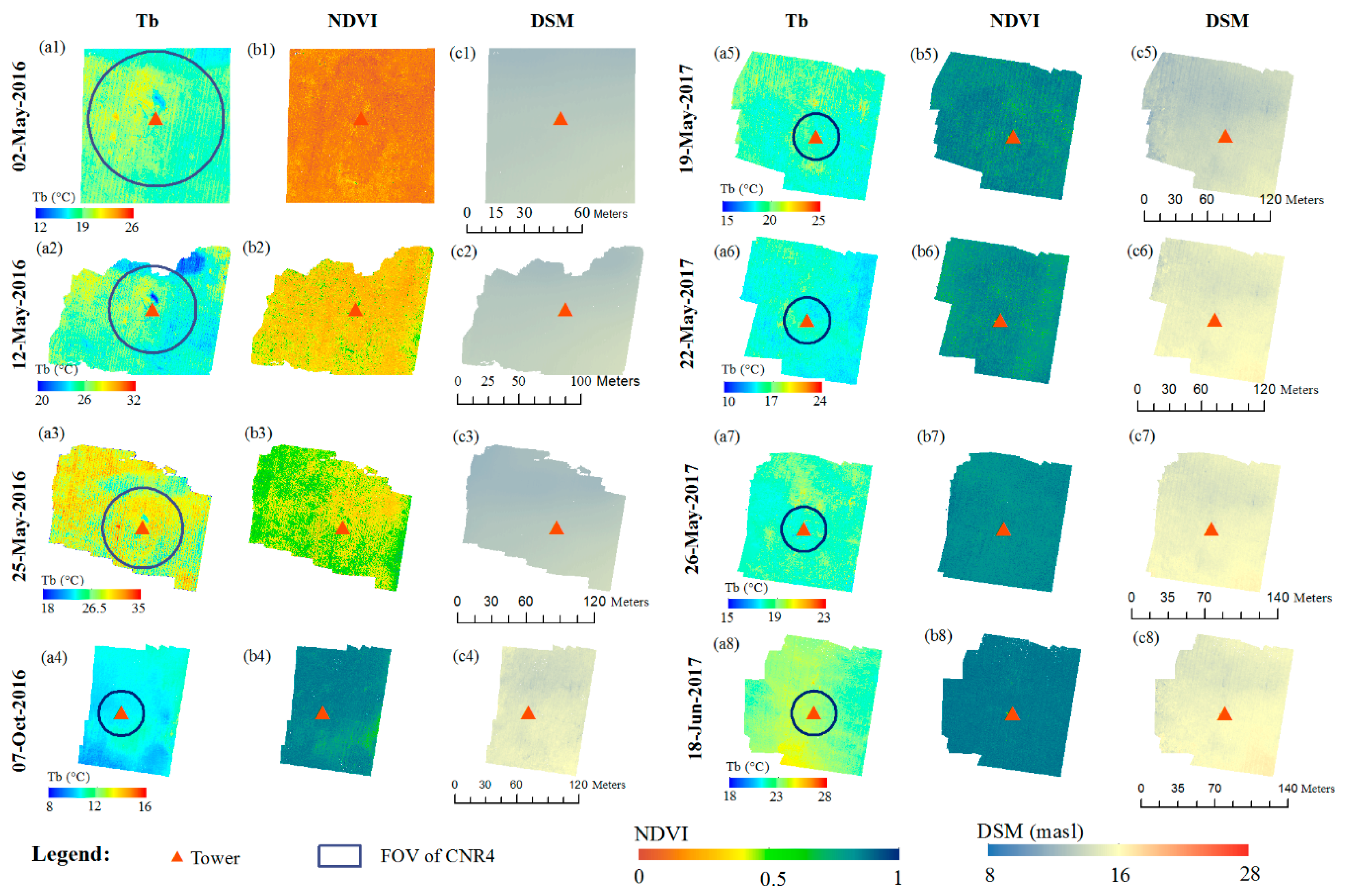
3.3. Image Processing and Validation

The workflow for image processing to obtain DSM, normalized difference vegetation index (NDVI), T_b and T_s (land surface temperature after emissivity correction) for this study is shown in Figure 3. The first step of image processing was to geo-reference images with GNSS data from UAS. Then, these georeferenced images along with pre-calibrated intrinsic camera geometric parameter values were imported into Agisoft Photoscan (Agisoft LLC, St. Petersburg, Russia) to generate orthophotos. Agisoft Photoscan software uses the structure-from-motion (SfM) approach [34] to generate orthomosaic and surface elevation maps from overlapping images from different positions and orientations. The Agisoft software firstly aligned images and generated sparse 3D point clouds. After that, high accuracy GCPs measured by the Trimble RTK GNSS were added to the aligned images. Then, the GNSS information from these accurate GCPs was used to optimize the image alignment by adjusting the estimated camera locations. Further, the DSM generated from RGB images was imported into both multispectral and thermal projects to orthorectify multispectral and thermal images. Finally, the six-band reflectance was calculated from the generated multispectral orthophotos based on the radiance method. An ASD spectroradiometer (FieldSpec HandHeld 2^TM Inc., Boulder, CO, USA) was used to collect with a Spectralon panel (nominal reflectance of 99.99%) before and after each UAS flight campaign. Then, the averaged spectral radiance was used as the incoming solar spectral radiance (${\mathrm{L}}_{\mathrm{in},\mathsf{\lambda }}$), while MCA measured the reflected spectral radiance for each band (${\mathrm{L}}_{\mathrm{MCA},\mathsf{\lambda }}$). Due to the low flight altitude, we did not conduct the atmospheric correction. Six-band reflectance was calculated as Equation (4). The reflectance of the near infrared (800 nm) and red (670 nm) bands was used to calculate NDVI as Equation (5).

$${\mathsf{\rho }}_{\mathsf{\lambda }}=\frac{{\mathrm{L}}_{\mathrm{MCA},\mathsf{\lambda }}}{{\mathrm{L}}_{\mathrm{in},\mathsf{\lambda }}}$$

(4)

$$\mathrm{NDVI}=\frac{{\mathsf{\rho }}_{800}-{\mathsf{\rho }}_{670}}{{\mathsf{\rho }}_{800}+{\mathsf{\rho }}_{670}}$$

(5)

where ${\mathrm{L}}_{\mathrm{MCA},\mathsf{\lambda }}$ is the reflected spectral radiance measured by MCA (W∙m⁻²∙sr⁻¹∙nm⁻¹), ${\mathrm{L}}_{\mathrm{in},\mathsf{\lambda }}$ is the incoming solar spectral radiance measured by ASD (W∙m⁻²∙sr⁻¹∙nm⁻¹), $\mathsf{\lambda }$ is the wavelength (nm). ${\mathsf{\rho }}_{800}$ is the reflectance at 800 nm, and ${\mathsf{\rho }}_{670}$ is the reflectance at 670 nm.

The observed fraction of vegetation cover ($f_{\mathrm{c}}$) as Equation (6) was calculated based on NDVI [39]. Further, the observed f_c (Equation (7)) was used to validate the estimated $f_{\mathrm{c}}$ from UAS ($f_{\mathrm{c}\_\mathrm{UAS}}$).

$$f_{\mathrm{c}\_\mathrm{UAS}}={\left(\frac{\mathrm{NDVI}-{\mathrm{NDVI}}_{\min }}{{\mathrm{NDVI}}_{\max }-{\mathrm{NDVI}}_{\min }}\right)}^2$$

(6)

$$f_{\mathrm{c}\_\mathrm{obs}}=\frac{{\mathrm{PAR}}_{\mathrm{above}}-{\mathrm{PAR}}_{\mathrm{reflected}}-{\mathrm{PAR}}_{\mathrm{below}}}{{\mathrm{PAR}}_{\mathrm{above}}}$$

(7)

where ${\mathrm{NDVI}}_{\max }=0.97$ for fully vegetated surface and ${\mathrm{NDVI}}_{\min }=0.24$ for bare soil were used in this study based on the field investigation. $f_{\mathrm{c}\_\mathrm{obs}}$ was calculated based on measurements of the incident PAR above the canopy (${\mathrm{PAR}}_{\mathrm{above}}$), canopy-reflected PAR (${\mathrm{PAR}}_{\mathrm{reflected}}$) and the average of eight understory PAR sensors (${\mathrm{PAR}}_{\mathrm{below}}$).

The T_b from the thermal orthophotos was influenced by the longwave radiation emitted by the object, the reflected longwave radiation and the atmospheric attenuation. UAS flight campaigns were conducted with a low attitude (Table 1), thus, in this study, we did not conduct atmospheric correction. To obtain the thermal signal emitted from the object (T_s), T_b was corrected with the land surface emissivity (ε_s) to exclude the signal from reflected longwave radiation as Equation (8). ε_s can be approximated based on an empirical relation with NDVI as Equation (9) [40].

$${\mathsf{\sigma }\mathrm{T}}_{\mathrm{b}}{}^4={\mathsf{\epsilon }}_{\mathrm{s}}{\mathsf{\sigma }\mathrm{T}}_{\mathrm{s}}{}^4+(1-{\mathsf{\epsilon }}_{\mathrm{s}}){\mathrm{LW}}_{\mathrm{in}}$$

(8)

$${\mathsf{\epsilon }}_{\mathrm{s}}=\{\begin{array}{ccc}0.986& & (\mathrm{NDVI}>0.608)\hfill \\ 1.0094+0.047\ln (\mathrm{NDVI})& & (0.131<\mathrm{NDVI}<0.608)\hfill \\ 0.914& & (\mathrm{NDVI}<0.131)\hfill \end{array}$$

(9)

where $\mathsf{\sigma }$ is the Stefan–Boltzmann constant (5.67 × 10⁻⁸ W∙m⁻²∙K⁻⁴), T_s is the surface temperature with emissivity correction (K), T_b is the brightness temperature from FLIR (K), and ${\mathrm{LW}}_{\mathrm{in}}$ is incoming longwave radiation (W∙m⁻²) and was calculated based on the Stefan–Boltzmann law using the atmospheric emissivity ε_a as Equations (10)–(13) [41].

$${\mathrm{LW}}_{\mathrm{in}}={\mathsf{\epsilon }}_{\mathrm{a}}{\mathsf{\sigma }\mathrm{T}}_a{}^4$$

(10)

$${\mathsf{\epsilon }}_{\mathrm{a}}=1-(1+\mathsf{\delta }){\mathrm{e}}^{-\sqrt{\left(1.2+3\mathsf{\delta }\right)}}$$

(11)

$$\mathsf{\delta }=\frac{46.5}{{\mathrm{T}}_{\mathrm{a}}}{\mathrm{e}}_0$$

(12)

$${\mathrm{e}}_0=\mathrm{RH}·6.11{\mathrm{e}}^{\left[\frac{{\mathrm{L}}_{\mathrm{v}}}{{\mathrm{R}}_{\mathrm{v}}}\left(\frac{1}{273.15}-\frac{1}{{\mathrm{T}}_{\mathrm{a}}}\right)\right]}$$

(13)

where ${\mathrm{e}}_0$ is the actual water vapor pressure (hPa) and was calculated based on the Clausius–Clapeyron equation, ${\mathrm{L}}_{\mathrm{v}}=2.5\times {10}^6\left(\mathrm{J}·{\mathrm{kg}}^{-1}\right)$ is the latent heat of vaporization, ${\mathrm{R}}_{\mathrm{v}}=461\left(\mathrm{J}·{\mathrm{kg}}^{-1}·{\mathrm{K}}^{-1}\right)$ is the gas constant for water vapor, and ${\mathrm{T}}_{\mathrm{a}}$ is the air temperature (K).

To check the accuracy of the generated DSM, the Trimble RTK GNSS was used to measure the ground elevation in different places across the site. It should be noted that the validation was mainly conducted during periods with low vegetation height (h_c < 0.5). During the dense vegetation period, we did not conduct validation, due to the difficulty in measuring the tree height.

To validate the acquired surface reflectance data, the reflectance of tarpaulins with four different colors (green, blue, black and silver) was measured with the ASD spectroradiometer for each flight. Tarpaulins are acknowledged to have low anisotropic effects [42]. The measured reflectance by ASD was used to validate reflectance from MCA. Validation was shown for 670 and 800 nm bands, since, in this study, only these two bands were used for calculating NDVI.

To conduct validation of the thermal infrared imagery in field conditions, the generated T_b orthophotos were compared with the brightness temperature converted from the outgoing longwave radiation (${\mathrm{LW}}_{\mathrm{out}\_\mathrm{CNR}4}$) from CNR4 on the tower (Figure 1). Even though FLIR and CNR4 have different thermal wavelength responses (FLIR: 7.5 to 13.5 μm, CNR4: 4.5 to 45 μm) and sensor FOVs (FLIR: 35° × 27°, CNR4: downward 150°), this comparison can provide insights into the quality of the thermal data to some extent. To compare with T_b from FLIR, ${\mathrm{LW}}_{\mathrm{out}\_\mathrm{CNR}4}$ was converted to brightness temperature T_{b_CNR4} by applying Stefan–Boltzmann’s law as Equation (14).

$${\mathrm{T}}_{\mathrm{b}\_\mathrm{CNR}4}={(\frac{{\mathrm{LW}}_{\mathrm{out}\_\mathrm{CNR}4}}{\mathsf{\sigma }})}^{1/4}$$

(14)

where $\mathsf{\sigma }$ is the Stefan–Boltzmann constant (5.67 × 10⁻⁸ W∙m⁻²∙K⁻⁴), ${\mathrm{T}}_{\mathrm{b}\_\mathrm{CNR}4}$ is the brightness temperature (K), and ${\mathrm{LW}}_{\mathrm{out}\_\mathrm{CNR}4}$ is the recoded longwave radiation by CNR4 (W∙m⁻²).

To get the corresponding pixels inside the FOV of CNR4, the flux tower position, the FOV and sensor height of CNR4, and the vegetation height were used to calculate the radius of the circle according to Equation (15), as one example, with the vegetation height equal to 0 m, as shown in Figure 1.

$$\mathrm{r}=(\mathrm{H}-{\mathrm{h}}_{\mathrm{c}})\tan (\frac{\mathrm{FOV}}{2})$$

(15)

where r is the radius of the projected sensor FOV on the surface (m), H is the sensor height (10 m), ${\mathrm{h}}_{\mathrm{c}}$ is the height of the willow plantation obtained from DSM (m), and FOV is the downward FOV of CNR4, namely 150°.

3.4. Temperature–Vegetation Triangle Approach

3.4.1. The Original “DT” Triangle Approach

Numerous satellite studies have applied the temperature–vegetation triangle approach to estimate both SM and evaporative fraction [11,18,21,22,28,29]. However, the linkage between applying the triangle approach for SM and evapotranspiration estimation is seldom explained. For SM estimation, originally, the temperature vegetation triangle index or soil wetness index (SWI) was defined as Equation (16), by rescaling the observed radiometric surface temperature (${\mathrm{T}}_{\mathrm{s},\mathrm{obs}}$) at each pixel between extreme dry and wet T_s for a given level of f_c [11,21,28] (hereinafter, “original triangle approach”). This approach assumed that the only factor modifying T_s in the triangle space apart from f_c is SM. The SWI is used to indicate SM conditions.

$$\mathrm{SWI}=\frac{{\mathrm{T}}_{\mathrm{s},\mathrm{obs}}-{\mathrm{T}}_{\mathrm{s},\mathrm{wet}}}{{\mathrm{T}}_{\mathrm{s},\mathrm{dry}}-{\mathrm{T}}_{\mathrm{s},\mathrm{wet}}}=\frac{{\mathrm{DT}}_{\mathrm{obs}}}{{\mathrm{DT}}_{\mathrm{dry}}}$$

(16)

$${\mathrm{DT}}_{\mathrm{dry}}=(1-f_{\mathrm{c}}){\mathrm{DT}}_{\mathrm{bs},\mathrm{dry}}$$

(17)

where the subscripts “dry”, “wet” and “obs” indicate dry, wet and observed conditions, respectively. ${\mathrm{T}}_{\mathrm{s},\mathrm{dry}}$ and ${\mathrm{T}}_{\mathrm{s},\mathrm{wet}}$ are the minimum and maximum T_s for a given f_c. For the wet edge, ${\mathrm{T}}_{\mathrm{s},\mathrm{wet}}$ corresponds to the temperature of the wet land surface and numerous studies proved that ${\mathrm{T}}_{\mathrm{s},\mathrm{wet}}$ is in equilibrium with T_a [22,36,43]. That means ${\mathrm{T}}_{\mathrm{s},\mathrm{wet}}$ can be replaced by T_a and DT_wet is equal to 0 [29]. DT_dry can normally be extracted from the observed dry edge in the triangle space. However, if there are no sufficient pixels to represent dry and wet conditions, DT_dry can be approximated from a linear mixture of ${\mathrm{DT}}_{\mathrm{bs},\mathrm{dry}}$ (temperature difference between the dry bare soil temperature and the air temperature) and DT_wet as Equation (17) [18,44].

The triangle approach can be quantitatively explained by the surface energy balance and one source evapotranspiration model [18,29], as shown in Figure 4. As shown in Figure 4b, the relationship between SM and Non-Evaporative Fraction (NEF = H/AE) for any given pixel within a fixed f_c can be described in a linear model approach Equation (18), due to the land–atmosphere coupling [1]. In Figure 4a, for a fixed level of f_c, the increases in T_s are due to increases in sensible heat flux (H), which are determined by decreases in SM.

$$\mathrm{NEF}=\frac{\mathrm{H}}{\mathrm{AE}}=1-\frac{\mathsf{\theta }-{\mathsf{\theta }}_{\mathrm{wt}}}{{\mathsf{\theta }}_{\mathrm{fc}}-{\mathsf{\theta }}_{\mathrm{wt}}}$$

(18)

where AE is the available energy and is equal to the sum of the sensible heat flux (H) and the latent heat flux (LE), $\mathsf{\theta }$ is the volumetric SM (m³∙m⁻³), ${\mathsf{\theta }}_{\mathrm{fc}}$ is the field capacity (m³∙m⁻³), and ${\mathsf{\theta }}_{\mathrm{wt}}$ is the wilting point of soil (m³∙m⁻³), representing the upper and lower limits of available SM [11].

For NEF, it can be further expressed as a ratio between H and H_dry as Equation (19). H_dry is the sensible heat flux at the dry edge, where LE is assumed to be negligible (Equation (20)). With the bulk sensible heat flux equation, H can be expressed as a ratio between DT and aerodynamic resistance (r_a). Further, if we assume that meteorological forcing and aerodynamic resistance (r_a) is constant within the area, NEF can further be simplified into a ratio between DT_obs and DT_dry by canceling the air density ($\mathsf{\rho }$), the specific heat of air at constant pressure (c_p) and aerodynamic resistance for heat transfer (r_a).

$$\mathrm{NEF}=\frac{\mathrm{H}}{\mathrm{AE}}=\frac{\mathrm{H}}{{\mathrm{H}}_{\mathrm{dry}}}=\frac{\frac{{\mathsf{\rho }\mathrm{C}}_{\mathrm{p}}{\mathrm{DT}}_{\mathrm{obs}}}{{\mathrm{r}}_{\mathrm{a},\mathrm{obs}}^{}}}{\frac{{\mathsf{\rho }\mathrm{C}}_{\mathrm{p}}{\mathrm{DT}}_{\mathrm{dry}}}{{\mathrm{r}}_{\mathrm{a},\mathrm{dry}}}}=\frac{\frac{{\mathrm{DT}}_{\mathrm{obs}}}{{\mathrm{r}}_{\mathrm{a},\mathrm{obs}}^{}}}{\frac{{\mathrm{DT}}_{\mathrm{dry}}}{{\mathrm{r}}_{\mathrm{a},\mathrm{dry}}}}\approx \frac{{\mathrm{DT}}_{\mathrm{obs}}}{{\mathrm{DT}}_{\mathrm{dry}}}$$

(19)

$${\mathrm{H}}_{\mathrm{dry}}=\mathrm{AE}=\frac{{\mathsf{\rho }\mathrm{C}}_{\mathrm{p}}{\mathrm{DT}}_{\mathrm{dry}}}{{\mathrm{r}}_{\mathrm{a}}^{}}$$

(20)

where DT_obs is the temperature difference between the surface and air for each pixel, DT_dry is the temperature difference for the dry pixel corresponding to a certain f_c level (Figure 4a), $\mathsf{\rho }$ is the air density (kg∙m⁻³), c_p is the specific heat of air at constant pressure (J∙kg⁻¹∙K⁻¹), r_a is the aerodynamic resistance for heat transfer (s∙m⁻¹), ${\mathrm{r}}_{\mathrm{a}\_\mathrm{obs}}^{}$ is the aerodynamic resistance for the observed pixel, and ${\mathrm{r}}_{\mathrm{a}\_\mathrm{dry}}$ is the aerodynamic resistance for the dry conditions.

In this way, we can explain the theories for using the triangle approach for both SM and evapotranspiration fraction (approximately 1-NEF). In this study, SWI (Equation (16)) was converted to the volumetric SM with a piecewise approach [11]. For energy limited evapotranspiration regime ($\mathsf{\theta }\ge {\mathsf{\theta }}_{\mathrm{fc}}$), SWI is equal to 0. For water limited, dry condition and no evapotranspiration conditions ($\mathsf{\theta }\le {\mathsf{\theta }}_{\mathrm{wt}}$), SWI is equal to 1. For water limited evapotranspiration regime (transitional conditions in Figure 4b) (${\mathsf{\theta }}_{\mathrm{wt}}<\mathsf{\theta }<{\mathsf{\theta }}_{\mathrm{fc}}$), the SWI can be expressed as Equation (21).

$$\mathrm{SWI}\approx 1-\frac{\mathsf{\theta }-{\mathsf{\theta }}_{\mathrm{wt}}}{{\mathsf{\theta }}_{\mathrm{fc}}-{\mathsf{\theta }}_{\mathrm{wt}}}$$

(21)

3.4.2. The Modified “DT/r_a” Triangle Approach

In a real-world condition, the assumption of the triangle approach may not be valid. For instance, if r_a is not homogeneous for a given f_c and causes variations in DT unrelated with SM, DT should be normalized with r_a, especially with fast surface elevation changes. In this study, the willow bioenergy plantation grows fast during the growing season and the change of h_c can alter the surface roughness to further affect DT. To exclude the influence of the change of surface roughness, we need to normalize DT with r_a for heat transfer. Thus, in this study (Equation (16)), we modified SWI to more accurately represent NEF as Equation (22) instead of Equation (16) for SM estimation.

$$\mathrm{SWI}=\frac{\frac{{\mathrm{DT}}_{\mathrm{obs}}}{{\mathrm{r}}_{\mathrm{a},\mathrm{obs}}^{}}}{\frac{{\mathrm{DT}}_{\mathrm{dry}}}{{\mathrm{r}}_{\mathrm{a},\mathrm{dry}}}}$$

(22)

To apply a modified triangle approach, we calculated an aerodynamic resistance and DT_dry. The aerodynamic resistance for heat transfer (${\mathrm{r}}_{\mathrm{a}}$) was calculated based on the algorithm proposed by Brutsaert (1982) as Equation (23) [45].

$${\mathrm{r}}_{\mathrm{a}}=\frac{\ln \left(\frac{\mathrm{z}-\mathrm{d}}{{\mathrm{z}}_{0\mathrm{m}}}\right)\ln \left(\frac{\mathrm{z}-\mathrm{d}}{{\mathrm{z}}_{0\mathrm{h}}}\right)}{{\mathrm{k}}^2\mathrm{u}}$$

(23)

$${\mathrm{z}}_{0\mathrm{h}}=\frac{{\mathrm{z}}_{0\mathrm{m}}}{{\mathrm{e}}^{{\mathrm{kB}}^{-1}}}$$

(24)

where z is the height of the reference wind velocity (m), i.e., the sensor height (10 m). To calculate ${\mathrm{r}}_{\mathrm{a},\mathrm{obs}}^{}$ in the real conditions, d is the zero-plane displacement height (m) and was chosen equal to 2/3 of $\overline{{\mathrm{h}}_{\mathrm{c}}}$. ${\mathrm{z}}_{0\mathrm{m}}$ is the surface roughness length for momentum transport and was equal to 0.1 of $\overline{{\mathrm{h}}_{\mathrm{c}}}$. $\overline{{\mathrm{h}}_{\mathrm{c}}}$ is the effective averaged h_c for the willow plantation. h_c was obtained by subtracting UAS-based DSM, which was obtained from each UAS flight campaign, with the digital elevation model (DEM). The DEM was obtained from UAS flight campaigns before the willow grew and only contained the elevation information of the ground surface (DSM without trees). ${\mathrm{z}}_{0\mathrm{h}}$ is the roughness lengths for heat transport and was calculated based on Equation (24). kB⁻¹ is a parameter to account for the local boundary resistance for the heat transfer and a constant value of 2.3 was adopted in this study [46]. k is von Karman constant (0.4). u is the horizontal wind speed at the reference height (m∙s⁻¹). For the dry bare soil conditions, d = 0 and ${\mathrm{z}}_{0\mathrm{m}}=0.005$ were used to calculate ${\mathrm{r}}_{\mathrm{a},\mathrm{dry}}$ in Equation (23) [47].

The dry edge, represented by DT_dry, cannot be extracted from the observed dry edge in the triangle space as UAS imagery does not have sufficient pixels to represent dry and wet conditions. Thus, we used ground meteorological observations to calculate theoretical dry edges. The dry edge ${\mathrm{DT}}_{\mathrm{dry}}/{\mathrm{r}}_{\mathrm{a},\mathrm{dry}}$ was obtained from a linear mixture of ${\mathrm{DT}}_{\mathrm{bs},\mathrm{dry}}/{\mathrm{r}}_{\mathrm{a},\mathrm{bs},\mathrm{dry}}$ (extreme dry bare soil conditions) and ${\mathrm{DT}}_{\mathrm{wet}}/{\mathrm{r}}_{\mathrm{a},\mathrm{wet}}$ (fully vegetated surface conditions). ${\mathrm{DT}}_{\mathrm{wet}}/{\mathrm{r}}_{\mathrm{a},\mathrm{wet}}$ can be approximated to 0, since the sensible heat flux for fully vegetated conditions is equal to 0 [18,44].

$$\frac{{\mathrm{DT}}_{\mathrm{dry}}}{{\mathrm{r}}_{\mathrm{a},\mathrm{dry}}}=(1-f_{\mathrm{c}})\frac{{\mathrm{DT}}_{\mathrm{bs},\mathrm{dry}}}{{\mathrm{r}}_{\mathrm{a},\mathrm{bs},\mathrm{dry}}}$$

(25)

For extremely dry bare soil conditions, LE is equal to 0. ${\mathrm{DT}}_{\mathrm{bs},\mathrm{dry}}$ can be derived based on the surface energy balance principle and the heat transfer equation as Equation (26) [44,47].

$${\mathrm{DT}}_{\mathrm{bs},\mathrm{dry}}=\frac{\left(1-\mathsf{\alpha }\right){\mathrm{SW}}_{\mathrm{in}}+{\mathsf{\epsilon }}_{\mathrm{ss}}{\mathsf{\epsilon }}_{\mathrm{a}}{\mathsf{\sigma }\mathrm{T}}_{\mathrm{a}}{}^4-{\mathsf{\epsilon }}_{\mathrm{s}}{\mathsf{\sigma }\mathrm{T}}_{\mathrm{a}}{}^4-\mathrm{LE}/\left(1-\mathrm{c}\right)}{4{\mathsf{\epsilon }}_{\mathrm{ss}}{\mathsf{\sigma }\mathrm{T}}_{\mathrm{a}}{}^3+{\mathsf{\rho }\mathrm{C}}_{\mathrm{p}}/\left[{\mathrm{r}}_{\mathrm{as}}\left(1-\mathrm{c}\right)\right]}$$

(26)

where ${\mathrm{SW}}_{\mathrm{in}}$ is the shortwave incoming radiation (W∙m⁻²) and, in this study, it was obtained from the meteorological tower. $\mathsf{\alpha }$ is the albedo of the dry bare soil and was adopted as 0.2 in this study according to the field investigation. ${\mathsf{\epsilon }}_{\mathrm{ss}}$ is the land surface emissivity for the dry bare soil (NDVI = 0.24) and the value of 0.94 was adopted according to Equation (10). ${\mathsf{\epsilon }}_{\mathrm{a}}$ is the emissivity for the atmosphere and was calculated based on Equation (10). $\mathsf{\sigma }$ is the Stefan–Boltzmann constant (5.67 × 10⁻⁸ W∙m⁻²∙K⁻⁴). LE was assumed to be 0 for the dry bare soil conditions. c is a ratio between the ground heat flux and net radiation. The value of 0.3 was adopted in this study [48]. $\mathsf{\rho }$ is the air density (kg∙m⁻³). ${\mathrm{C}}_{\mathrm{p}}$ is the specific heat of air at constant pressure (J∙kg⁻¹∙K⁻¹).

3.5. Sensitivity Test of the Modified Triangle Approach to the Canopy Height

To investigate the sensitivity of the proposed “DT/r_a” triangle approach to h_c, a sensitivity test to model inputs (h_c, DT and f_c) was conducted. The atmospheric forcing was based on 26 May 2017 and there were two experiments in the test. The first experiment was to control f_c and quantified the relationship between h_c and SWI with different DT. A pixel was assumed to be f_c equal to 0.5, h_c from 0.1 to 3 m with an interval of 0.01 m, and DT from 0 to 5 °C with an interval of 1 °C. The second one was to control DT, which was assumed to be equal to 1 °C, and explored the relationship between h_c and SWI with different levels of f_c. A pixel was assumed to have h_c from 0.1 to 3 m with a 0.01 m interval and f_c from 0 to 1 with a step of 0.1. Totally, 3492 simulations were conducted. Then, these results were used to analyze the sensitivity of the “DT/r_a” approach to h_c, DT and f_c. This sensitivity analysis quantified the sensitivity of model inputs. Further, with the information of input uncertainty from the validation of UAS observations, this analysis could also provide insights into the uncertainty of the simulated SWI.

3.6. Validation of Soil Moisture Estimates

The estimated SWI was converted to the volumetric soil moisture ($\mathsf{\theta }$) as Equation (22) with ${\mathsf{\theta }}_{\mathrm{fc}}$ and ${\mathsf{\theta }}_{\mathrm{wt}}$ equal to 0.31 and 0.15, respectively. The values of ${\mathsf{\theta }}_{\mathrm{fc}}$ and ${\mathsf{\theta }}_{\mathrm{wt}}$ were determined according to the soil texture (loam) and long-term in-situ SM observations from 2012 to 2017. Here, we use the “DT” and “DT/r_a” to denote the original and modified triangle approaches, respectively. In-situ SM observations from the portable and fixed SM sensors were used to validate the spatial and temporal dynamics of estimated SM from these two approaches. The Root Mean Square Deviation (RMSD, Equation (27)), Correlation Coefficient (R, Equation (28)), Relative Error (RE, Equation (29)), unbiased Root Mean Square Deviation (ubRMSD, Equation (30)) and Standard Deviation (STD, Equation (31)) were used as statistical indices to evaluate the performance of estimated SM. The Taylor diagram (Taylor, 2001), which presents the complementary statistics among R, Normalized STD (NSTD, as Equation (32)) and Normalized ubRMSD (NubRMSD), was used. In the Taylor diagram, these three statistical indices have a triangle-cosine-law-like relationship, as Equation (33). The radial distance of the diagram stands for the NSTD and the angle in the polar plot represents R. The reference point located on the x-axis with R = 1, NSTD = 1, and NubRMSD = 0 is the observation. The distance from the simulation point to the reference point means the NubRMSD of simulations and it is the integrated performance of the simulation.

$$\mathrm{RMSD}=\sqrt{{\displaystyle \sum _{\mathrm{i}=1}^{\mathrm{N}}}{\left({\mathrm{sim}}_{\mathrm{i}}-{\mathrm{obs}}_{\mathrm{i}}\right)}^2/\mathrm{N}}$$

(27)

$$\mathrm{R}=\frac{{\sum }_{\mathrm{i}=1}^{\mathrm{N}}\left({\mathrm{sim}}_{\mathrm{i}}-\overline{\mathrm{sim}}\right)\left({\mathrm{obs}}_{\mathrm{i}}-\overline{\mathrm{obs}}\right)}{\sqrt{{\sum }_{\mathrm{i}=1}^{\mathrm{N}}{\left({\mathrm{sim}}_{\mathrm{i}}-\overline{\mathrm{sim}}\right)}^2}\sqrt{{\sum }_{\mathrm{i}=1}^{\mathrm{N}}{\left({\mathrm{obs}}_{\mathrm{i}}-\overline{\mathrm{obs}}\right)}^2}}$$

(28)

$$\mathrm{RE}=\left(\overline{\mathrm{sim}}-\overline{\mathrm{obs}}\right)/\overline{\mathrm{obs}}$$

(29)

$$\mathrm{ubRMSD}=\sqrt{{\displaystyle \sum _{\mathrm{i}=1}^{\mathrm{N}}}{\left[\left({\mathrm{sim}}_{\mathrm{i}}-\overline{\mathrm{sim}}\right)-\left({\mathrm{obs}}_{\mathrm{i}}-\overline{\mathrm{obs}}\right)\right]}^2/\mathrm{N}}$$

(30)

$$\mathrm{STD}=\sqrt{{\displaystyle \sum _{\mathrm{i}=1}^{\mathrm{N}}}{\left(\mathrm{sim}-\overline{\mathrm{sim}}\right)}^2/\mathrm{N}}$$

(31)

$${\mathrm{NSTD}}_{\mathrm{sim}}={\mathrm{STD}}_{\mathrm{sim}}/{\mathrm{STD}}_{\mathrm{obs}}$$

(32)

$${\mathrm{NubRMSD}}_{\mathrm{obs},\mathrm{sim}}^2={\mathrm{NSTD}}_{\mathrm{obs}}^2+{\mathrm{NSTD}}_{\mathrm{sim}}^2-2{\mathrm{NSTD}}_{\mathrm{obs}}{\mathrm{NSTD}}_{\mathrm{sim}}\cos {\mathrm{CC}}_{\mathrm{obs},\mathrm{sim}}$$

(33)

where sim is the simulation, obs is the observation, i refers to the i^th simulation or observation, N is the total number of data points, $\overline{\mathrm{sim}}$ is the average of the simulation, and $\overline{\mathrm{obs}}$ is the average of the observation.

A scale discrepancy may exist between pixel-based UAS imagery and point-based in-situ SM measurements. In the spatial validation, to compare with in-situ measurements, we used the mean values from buffer zones (circles) of different radiuses around the sample location in UAS imagery. In the temporal validation, we compared the estimated SM and in-situ measurements at different soil depths.

4. Results

4.1. UAS Sensor Calibration and Data Validation

Results of pixel-wise calibration in the laboratory are shown in Figure 5. With the pixel-wise calibration, the RMSDs of the thermal imagery were less than 0.57 °C. The nearly uniform pattern indicates that, through the calibration, the typical camera image errors, e.g., vignetting effects, were removed. The orthophotos of T_b, NDVI, and DSM obtained from UAS flight campaigns are shown in Figure 6. It can be found that the first three flights of 2016 were obtained at the beginning of the growing season with NDVI < 0.5 and DSM < 15.5 m, while the last five flights have more dense vegetation with NDVI > 0.7 and DSM around 16–18 m.

To check the quality of these orthophotos, T_b, reflectance and DSM were compared with in-situ observations (Figure 7). Comparison between the UAS T_b and CNR4 T_b showed a close correspondence between the brightness temperatures with R² equal to 0.97 and RMSD of 0.93 °C. Figure 7b indicates a good accuracy of the reflectance at 670 and 800 nm with R² more than 0.98 and RMSD less than 3%. Figure 7c shows the accuracy of the generated DSM from the RGB images. The RMSD of the DSM is 0.06 m from three campaigns in May 2016 when the willow plants had a small growth height (h_c < 0.5 m). Validation of f_c (Figure 7d) revealed a good correspondence with the observations with R² equal to 0.99 and RMSD of 0.04.

4.2. Sensitivity of the Modified Triangle Approach to the Vegetation Height

Figure 8 shows the modified triangle approach is sensitive to the change of h_c, DT and f_c. In general, in the same conditions of the observed DT and f_c, the higher h_c corresponds to higher SWI. Figure 8a shows that, with the same level of SWI and f_c, the higher DT corresponds to the higher h_c. This agrees with the fact that, for pixels with the same SM, f_c and atmospheric conditions, pixels with a higher h_c tend to have higher surface roughness and lower r_a. Similarly, as shown in Figure 8b, with the same levels of f_c and DT, the pixels with higher h_c correspond to higher SWI. Different from the sensitivity of SWI to DT with the same level of h_c, which is approximately linear, the sensitivity of SWI to f_c with the same h_c is highly non-linear. In low f_c conditions, the sensitivity of SWI to f_c is low, while it is much higher in the high f_c conditions. Within the same levels of DT and f_c, the sensitivity of SWI to h_c is closer to linear.

Further, Figure 8 also provides insights into simulation uncertainty of this study. As shown in the validation of UAS orthophotos (Figure 7), with the pixel-wise calibration approach, UAS-based T_s can have an uncertainty around 0.93 °C in the field. The RMSD of reflectance is around 3% and the RMSD of h_c is about 0.06 m. It should be noticed that RMSD of h_c is assessed when h_c < 0.5 m and errors for high h_c conditions is likely to be higher. Here, we use 0.5 m to consider the uncertainty of h_c. In Figure 8a, for instance, with the condition DT = 1 °C and f_c = 0.5, the uncertainty of 0.5 m in h_c can contribute to the uncertainty of SWI around 0.02. With the condition f_c = 0.5 and h_c = 2 m, the 1 °C uncertainty of T_s can contribute to the uncertainty of SWI about 0.15. As for f_c in Figure 8b, with the condition DT = 1 °C and h_c = 1 m, it can contribute to the uncertainty of SWI around 0.05 in low f_c conditions (f_c < 0.5), while the uncertainty of SWI is much higher in high f_c conditions. Therefore, in this approach, the accuracy of SWI is highly sensitive to DT and, in high f_c conditions, it is also highly sensitive to f_c.

4.3. Spatial Validation of UAS Estimated Soil Moisture

The spatial patterns of the estimated SWI from the two triangle approaches (“DT” and “DT/r_a”) are shown in Figure 9(a1–a8) and (b1–b8), respectively. It can be seen that before the willow grew (the first three flights of 2016), there was no difference in spatial patterns and histogram distributions between “DT” and “DT/r_a” as shown in Figure 6(a1–a3) and (b1–b3). However, when the willow grew up (the last five flights) and the canopy grew higher, the spatial patterns of SWI from these two approaches became different. In the “DT/r_a” approach, the normalization of r_a tends to stretch SWI of willow plantation to a higher value. From the histogram distributions (Figure 9(c4–c8)), it can also be seen that, after normalization, more pixels have higher values of SWI.

The corresponding T_s-f_c scatterplots for these UAS flights are shown in Figure 10. From the scatterplots, it is clear that there is a large mismatch between the observed dry and wet edges and the theoretical ones, since UAS campaigns do not have a large coverage of heterogeneous landscapes to represent the dry and wet edges. This confirms that it is necessary to calculate the theoretical dry and wet edges for the triangle approach. It should also be noticed that, in the scatterplots, there are outliers in the feature space enclosed by the theoretical dry and wet edges. This can be attributed to the difference between aerodynamic and radiometric temperatures [49] or errors in the retrieval of T_s from the UAS sensors. Due to the lower r_a of the willow plantation than the pixels of grass or bare soil, after normalization, points in the “DT/r_a” approach shifted toward the dry edge as compared to the “DT” approach (Figure 10). This also agrees with the change of the spatial pattern and the histogram distribution in Figure 9.

Figure 11 shows the spatial validation of “DT” and “DT/r_a” approaches with different buffer zone sizes. Because the h_c was calculated based on the averaged h_c, the normalization did not change the correlation coefficient R. However, it can also be seen that there was a significant improvement in RMSD and relative errors (RE) with normalized r_a than without. With a buffer zone of 1.5 m radius, as shown in Figure 11g, on 26 May 2017, the RE reduced from 14.02% to −1.51%. Similarly, on 18 June 2017, as shown in Figure 11h, the RMSD decreased from 0.04 to 0.02 m³·m⁻³ and the RE reduced from 15.07% to −2.53%. Further, the comparison between different sizes of buffer zones indicates that the best match of R between SWI and in-situ SM measurements was with buffer zones of 1.5 m radius.

4.4. Temporal Validation of UAS Estimated Soil Moisture

Figure 12 shows the temporal variations of in-situ and UAS derived SM estimates for Soil Profile A (Figure 1) during the growing seasons of 2016 and 2017. In the non-growing season (November–April), this site had high SM and was energy limited, while, during the growing season (May–October), the condition switched to SM limited (Figure 4). This supports the assumption of this study to apply NEF to estimate SM during the growing season. By comparing the “DT” and “DT/r_a” approaches, we found that SM estimates from the “DT/r_a” scheme had a close correspondence with the temporal variations of in-situ SM measurements at depths of 15 and 30 cm.

The Taylor diagram and the scatterplot (Figure 13) shows the temporal validation of the “DT” and “DT/r_a” approaches with SM at different depths (5, 15, 30 and 60 cm) for Soil Profiles A and B (Figure 1) with 1.5 m buffer zones. Significant improvements in R by normalizing r_a is evident than without normalization. In the Taylor diagram (Figure 13a), all markers representing “DT/r_a” approach (solid colors) had closer correspondence to the observation than markers representing the “DT” approach. Compared to the “DT” approach, R of the “DT/r_a” approach increased from −0.25–0.1 to approximately 0.4–0.75. The “DT/r_a” approach had the best matches with the in-situ SM at 15 and 30 cm depth, which corresponds to the root-zone depth of the willow plantation [50]. The R between the SM estimates and observations at the depth of 15 and 30 cm improved from the value around 0 (not significant correlation) to 0.7 (<0.05 significance level). Similarly, in Figure 13b, the comparison shows the “DT/r_a” approach had the lowest RMSD around 0.025 m³∙m⁻³ and RE about 3% when compared with the SM at 15 and 30 cm. However, in the “DT” approach, RMSDs were around 0.045 m³∙m⁻³ and REs were about 10%. Generally, the improvement for the “DT/r_a” approach in the temporal domain was substantially larger than the comparison in the spatial domain. This is because, in the temporal domain, h_c changed more significantly from 0 to approximately 4 m. Further, regarding SM measurements at different depths, it can be found that the estimated SM from the triangle approach has better correlation with measurements at 15–30 cm depths, as shown by the green and light blue symbols in Figure 13. These results suggest that the estimated SM from the triangle approach reflects SM at the root zone.

5. Discussion

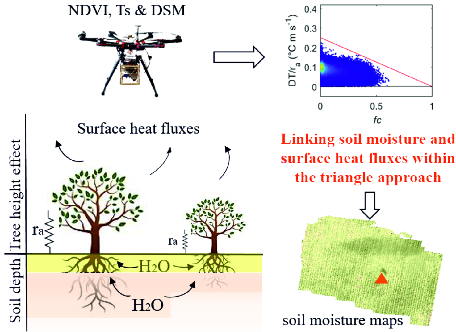
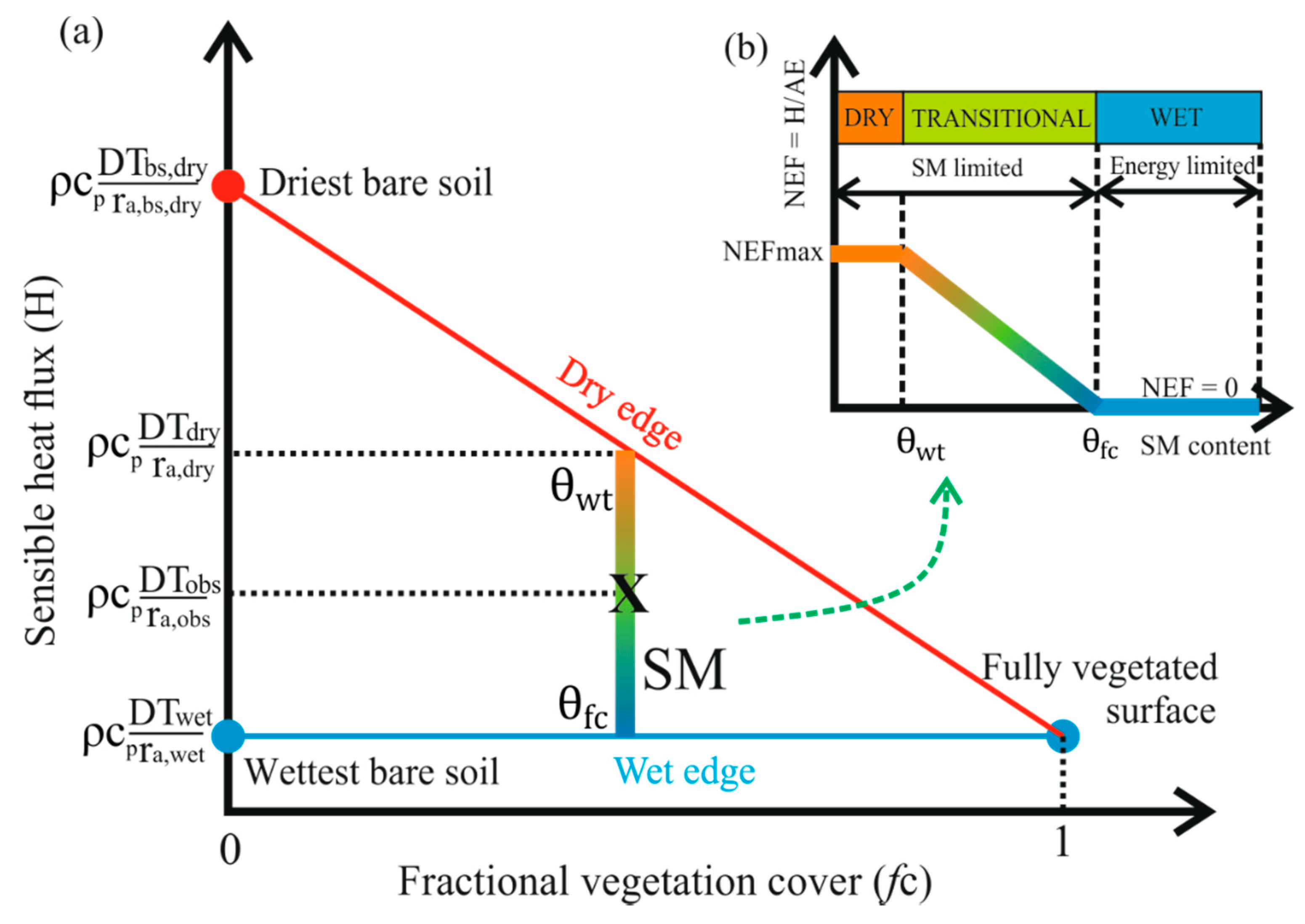
5.1. Linking Soil Moisture, Surface Heat Flux and the Triangle Approach

The temperature–vegetation triangle space is defined by the scatterplot of surface temperature (assuming a constant air temperature) and vegetation cover, where the triangle boundaries correspond to dry and wet endmembers of SM (Figure 4). In this 2D space, the relative position of an observation of surface temperature between the wet/dry extremes has already been extensively applied to map SM using satellite data and at spatial scales of 60 m to 1 km [11,21,28]. Using high resolution imagery from UASs provides opportunity to match the typical spatial scale of SM variations (meter level) [51], identify areas of low SM levels where water is limiting for plants and will be obscured in coarser grids [52], and also interpret how fluxes aggregate within a footprint of the EC system.

In our study, we mapped changes in SM over a willow forest at canopy scales by considering a simple piecewise SM relation with sensible heat flux normalized by available energy at the scale of tree crowns (Figure 4) [1,53] together with observations of T_s and f_c. The linkage between soil moisture and surface heat flux within the triangle approach shows that using a triangle approach for mapping SM requires considering any environmental factors susceptible to modify T_s (vertical axis of Figure 4) other than SM [11,21,28,29]. As it happens in our study site, it is possible that pixels with the same fractional cover have different aerodynamic properties due to tree height variations. In this framework, finding the absolute or “exact” value of the aerodynamic resistance is less important than accounting for relative variations among pixels with the similar vegetation cover, not being as critical as in SEB models that explicitly estimate sensible heat flux using aerodynamic resistances [54]. Additionally, as the aerodynamic properties of soil and vegetated surfaces are quite different, just accounting for those in the triangle for the full cover and bare soil cases corrected most of the original bias (spatial validation in Figure 11 and temporal validation in Figure 13). To do that, we used the formulation of bulk aerodynamic resistance under neutral conditions from Brutsaert with roughness effective parameters similar to Moran et al. (1994) and Hoffman et al. (2016) [16,18]. In their studies, those parameters were derived from static prescribed crop height for the entire area, while we used estimates of tree height derived from SfM photogrammetry techniques, which is a more accessible alternative to LiDAR to retrieve canopy structure information [55]. To have effective parameters of roughness length at blending height for momentum and displacement height, we averaged tree height (e.g., roughness elements) over the footprint area in each date. The SM retrieved showed larger improvements in accuracy over time more than over space. This is logical, as we did not consider the effect of fine scale spatial variability (canopy level) and because the tree height variation is very high (0–4 m) over time in this willow forest.

5.2. Influence of the 3D Canopy Structure to the Triangle Approach at Fine Resolution

The main improvement of SM estimates is on the temporal domain, in which h_c changes from 0 to around 4 m. In the spatial domain, there was an improvement in RMSD and RE, but no changes in the correlation coefficient. This is due to that the averaged h_c from the whole willow patch was used to calculate the bulk aerodynamic roughness and a constant kB⁻¹ of 2.3 was used to account for the local boundary resistance for the heat transfer. An important aspect to further improve the triangle approach is the proper interpretation of the spatial patterns of T_s detected from UAS at fine scales of ~1 m [56]. These fine spatial T_s patterns vary in response to the water status of tree crowns, as trees modify root-zone SM through transpiration [52]. However, the spatial patterns are also influenced by the micro-scale structural heterogeneity of forest canopies due to gaps or tree height changes [57]. Historically, it has been considered that turbulence mixing “wipes” out such fine scale heterogeneities, but it has been shown that the eddy mixing length inside and just above the canopy sublayer is at the same scale as the tree-crown diameter and, therefore, crown-scale heterogeneity leads to persistent effects [57,58]. In fact, the spatial arrangement of soil and vegetation patches and plant architecture produces near-surface turbulent changes clearly modifying the surface fluxes and not accounted for in turbulent diffusion theory formulations [56,59].

Typically, the effect of tree scale heterogeneity when calculating turbulent fluxes is accounted via length scales using a scalar quantity (zero plane displacement and aerodynamic roughness length) that aim to account for the 3D effects of the canopy structure on the momentum transfer, using effective patch-averaged profiles when the goal is to estimate the fluxes at the blending height as we also did over time [57]. However, in this study, a zero-dimensional representation of 3D canopy effects using uniform scalar properties removes the signature of heterogeneity on fluxes and temperature when heterogeneity is relevant as in the case of mapping fine scale SM patterns.

One simple possibility to incorporate the effect of canopy heterogeneity in the triangle space would be to consider an additional boundary layer resistance to heat transport in series with the aerodynamic resistance, to account for variations in heat transfer due changes in tree height that would modify heat roughness length as in Equations (34) and (35). That means that, in Equations (34) and (35), the averaged $\overline{{\mathrm{h}}_{\mathrm{c}}}$ can be used to estimate z_om, while the pixel h_c can be used to calculate z_oh. Thus, the effective spatially-averaged h_c is used for the aerodynamic resistance between the reference height and the displacement height and the local variation of h_c with respect to the average h_c is used to account for the local boundary resistance for Z_oh. In practice, this is equivalent to calculating a kB⁻¹ resistance that is dependent on tree height.

$${\mathrm{z}}_{0\mathrm{h}}=0.1\overline{{\mathrm{h}}_{\mathrm{c}}}$$

(34)

$${\mathrm{z}}_{0\mathrm{h}}=0.1(\overline{{\mathrm{h}}_{\mathrm{c}}}+·{\mathrm{h}}_{\mathrm{c}})$$

(35)

where $\overline{{\mathrm{h}}_{\mathrm{c}}}$ is the averaged canopy height for the willow planation and $·{\mathrm{h}}_{\mathrm{c}}$ is the local variation of the canopy height.

To explore if accounting for the spatial variability of h_c had an impact on the retrieval of SM, we compared the local h_c formulation of Equation (34) with the two prior approaches (no resistance DT and effective parameterized resistance DT/r_a with average h_c) on 18 June 2017 as it had more TDR measurements available. The results are shown in

Table 2. Comparison of the approaches to consider the spatial variations of the canopy height (the spatial validation was on 18 June 2017).

Approach		R	RMSD (m3∙m−3)	RE (%)
DT		0.67	0.04	15.07
DT/ra	average hc	0.67	0.02	2.53
DT/ra	Local hc for kB−1	0.69	0.02	1.84

. It can be seen that, when including local variations of h_c at the pixel level, there is a slight improvement. This indicates the variation of h_c inside the plantation is also important, even though the spatial variations are not that large. It can be expected that, for other sites with larger spatial variations of h_c, more significant improvement could be achieved.

The aerodynamic roughness length in this study was expressed as a ratio of h_c [45]. This is valid for homogeneous surfaces as the eddy covariance flux site of this study [33]. However, for the heterogeneous landscapes, additional consideration of the effective averaged obstacle height and frontal area index can help to obtain more accuracy [58]. Moreover, h_c can also be more accurately acquired from UAS LiDAR techniques. For instance, the comparison between UAS-based LiDAR and SfM techniques shows that LiDAR is relatively more accurate in the forest height and 3D structure detection, while SfM is an adequate low-cost alternative [60].

Another aspect related with SM retrieval from the relation with surface heat fluxes is due to the fact that every tree has a different root system and root depth; therefore, T_s pattern will respond to slightly different SM levels from tree to tree. That might explain why we get the better correlations in the layers with higher root density. It can be expected that, in this study, during the progress of the growing season from bare soil to full canopy cover, UAS-based SWI is associated with SM in different depths. For the bare soil period, SWI indicates SM more superficial, while for high canopy covers, SWI was related with SM at deeper depths. Since this study has more UAS observations with high canopy covers (f_c > 0.7) over Soil Profiles A and B, it explained better correlations with SM at layer around 15–30 cm depths. This finding agrees with other studies that showed SM estimates from the triangle approach to be more related to the root-zone SM [19,61]. For instance, Wang et al. (2018) compared the SM estimates from UAS with in-situ SM at different depths at the experimental plots with spring wheat and found the best match between estimates and observations to be at 10–20 cm depth, which corresponds to the root zone of the wheat [19].

The comparison between different sizes of buffer zones indicates that the best match of R was with buffer zones of 1.5 m radius. Several reasons can justify the best match at this size of buffer zones. The triangle approach infers SM through canopy temperature for high f_c levels. Although UAS imagery provided sub-meter level VHR imagery of the canopy, there may be a spatial discrepancy between the canopy status and SM conditions underneath the canopy. This means the detected canopy status may reflect the SM conditions representing the few meters around the canopy instead of the SM condition just below the canopy and, in fact, the root of the willow plantation can spread 1–3 m around the tree [62]. Further, a complete canopy is composed of sunlit and shaded leaves and a single pixel among the canopy cannot reflect the whole status of the canopy and SM conditions in the root zone [63]. According to the DSM and visual inspection of the RGB photos, as shown in Figure 1, the radiuses of the canopy are around 1–1.5 m in dense vegetation conditions. This approximately agrees with the size of the buffer zones. Additionally, there are uncertainties in the georeferencing of the UAS image processing and the Trimble RTK GNSS, which was used to measure the location of TDR measurements and GCPs, also has errors. Therefore, errors were reduced with spatial aggregation.

5.3. Comparison with Other Studies

While numerous studies have been conducted with thermal inertia, the triangle approach and microwave to estimate SM from satellite and manned airborne remote sensing [11,36,63,64], only few studies have been conducted with UAS observations [4,17,19]. For instance, Sobrino et al. (2012) used NDVI and T_s with a polynomial formulation to predict SM and this approach can estimate SM with RMSDs of 0.05 m³∙m⁻³ from observations from a manned airborne system [64]. Fan et al. (2015) used vegetation indices and T_s to estimate SM with RMSDs around 0.023 m³∙m⁻³ from a manned airborne system [63]. Wang et al. (2018) demonstrated that UAS-based optical and thermal remote sensing data can be utilized with the water deficit index approach to estimate SM with R² reaching to 0.63 and RMSDs less than 0.1 m³∙m⁻³ [19]. Compared to these studies, this study achieved an accuracy to map spatial and temporal variations of SM with R around 0.58–0.69 and RMSDs around 0.025 m³∙m⁻³. Further, this study was based on the triangle approach to utilize the optical and thermal remote sensing information. It has advantages to be applied for bare soil, sparse and dense vegetation conditions. Moreover, this approach can be applied to monitor the root-zone SM, which has added significance for predicting near-future vegetation anomalies [65]. Further, the approach of this study does not need parameter calibration and most inputs were available from UAS observations. This UAS-based SM monitoring approach can be applied in the data-scarcity regions. However, the shortage of this method is that, in the dense vegetation conditions, the accuracy of this method is very sensitive to the accuracy of the optical and thermal data, as shown in Figure 8. For the miniaturized UAS thermal sensors, it is hard to obtain surface temperature with very high accuracy (<1 °C). Thus, the precise calibration of the thermal sensor, as performed in this study, is recommended. Additionally, novel trapezoid methods utilizing the visible and shortwave infrared data may be another alternative [66,67].

6. Conclusions

In this study, an operational methodology to map soil moisture (SM) in the root-zone at high spatial resolution (m level) from Unmanned Aerial Systems (UAS) is proposed. We improved the state-of-the-art temperature-vegetation triangle methodology by normalizing the land–atmosphere temperature gradients with a bulk aerodynamic resistance that was derived from structure-from-motion based surface elevation maps. In this way, the effects of the tree growth driven surface roughness dynamics on surface temperatures were considered. Due to the limited coverage of the UAS, the hydrological contrast of the UAS maps was reduced, which lead us to model theoretical dry and wet edges rather than extracting them from the images. Evaluation with SM measurements in a Danish bioenergy willow short rotation coppice in two consecutive summer seasons led us to the following conclusions:

(i)

Accounting for changes in surface roughness considerably increased the performance of the temperature-vegetation triangle approach to estimate SM variation.

(ii)

Under densely vegetated conditions, the estimated SM from the triangle approach correlated better with the root-zone SM than with the surface SM (< 10 cm). This shows that the modified triangle approach is better suited to monitor water availability for vegetation compared to thermal inertia- or microwave-based approaches, which detect surface rather than deeper root-zone SM.

(iii)

The optimum spatial resolution or aggregation for the modified triangle approach is in the same order of magnitude as the typical length scale of the tree crowns.

(iv)

Given the high sensitivity of SM model to errors in surface temperature estimates, we proposed a pixel-wise sensor calibration method to improve the accuracy of the uncooled UAS thermal sensor to be around 0.55 °C for the laboratory conditions and 0.95 °C in the field.

(v)

The proposed methodology mainly relies on UAS observations and requires limited in-situ measurements, e.g., solar incoming radiation, air temperature and humidity, wind speed, and atmospheric pressure, and can be operationally used for routine SM monitoring in both agricultural and natural ecosystems.

This study mainly addresses the influence of the temporal changes of the canopy roughness on the triangle approach. Future research should consider the effects of strong spatial variation of the canopy height and the role of canopy gaps for the fine scale patterns of the surface temperature observed from UAS, to avoid contamination of the estimated SM maps by micro-scale variability of structural induced turbulence patterns and radiation budgets.

References

1. Seneviratne, S.I.; Corti, T.; Davin, E.L.; Hirschi, M.; Jaeger, E.B.; Lehner, I.; Orlowsky, B.; Teuling, A.J. Investigating soil moisture-climate interactions in a changing climate: A review. Earth-Science Rev. 2010, 99, 125–161. [Google Scholar] [CrossRef]
2. Sheffield, J.; Wood, E.F.; Chaney, N.; Guan, K.; Sadri, S.; Yuan, X.; Olang, L.; Amani, A.; Ali, A.; Demuth, S.; et al. A drought monitoring and forecasting system for sub-sahara african water resources and food security. Bull. Am. Meteorol. Soc. 2014, 95, 861–882. [Google Scholar] [CrossRef]
3. Qiu, J.; Gao, Q.; Wang, S.; Su, Z. Comparison of temporal trends from multiple soil moisture data sets and precipitation: The implication of irrigation on regional soil moisture trend. Int. J. Appl. Earth Obs. Geoinf. 2016, 48, 17–27. [Google Scholar] [CrossRef] [Green Version]
4. Hassan-Esfahani, L.; Torres-Rua, A.; Jensen, A.; McKee, M. Assessment of surface soil moisture using high-resolution multi-spectral imagery and artificial neural networks. Remote Sens. 2015, 7, 2627–2646. [Google Scholar] [CrossRef]
5. Andreasen, M.; Jensen, K.H.; Desilets, D.; Franz, T.E.; Zreda, M.; Bogena, H.R.; Looms, M.C. Status and Perspectives on the Cosmic-Ray Neutron Method for Soil Moisture Estimation and Other Environmental Science Applications. Vadose Zo. J. 2017, 16, 0. [Google Scholar] [CrossRef]
6. Van Doninck, J.; Peters, J.; De Baets, B.; De Clercq, E.M.; Ducheyne, E.; Verhoest, N.E.C. The potential of multitemporal Aqua and Terra MODIS apparent thermal inertia as a soil moisture indicator. Int. J. Appl. Earth Obs. Geoinf. 2011, 13, 934–941. [Google Scholar] [CrossRef]
7. Petropoulos, G.; Carlson, T.N.; Wooster, M.J.; Islam, S. A review of Ts/VI remote sensing based methods for the retrieval of land surface energy fluxes and soil surface moisture. Prog. Phys. Geogr. 2009, 33, 224–250. [Google Scholar] [CrossRef]
8. Dorigo, W.A.; Scipal, K.; Parinussa, R.M.; Liu, Y.Y.; Wagner, W.; De Jeu, R.A.M.; Naeimi, V. Error characterisation of global active and passive microwave soil moisture datasets. Hydrol. Earth Syst. Sci. 2010, 14, 2605–2616. [Google Scholar] [CrossRef] [Green Version]
9. Petropoulos, G.P.; Ireland, G.; Barrett, B. Surface soil moisture retrievals from remote sensing: Current status, products & future trends. Phys. Chem. Earth 2015, 83–84, 36–56. [Google Scholar] [CrossRef]
10. Njoku, E.G.; Jackson, T.J.; Lakshmi, V.; Chan, T.K.; Nghiem, S.V. Soil moisture retrieval from AMSR-E. IEEE Trans. Geosci. Remote Sens. 2003, 41, 215–228. [Google Scholar] [CrossRef]
11. Mallick, K.; Bhattacharya, B.K.; Patel, N.K. Estimating volumetric surface moisture content for cropped soils using a soil wetness index based on surface temperature and NDVI. Agric. For. Meteorol. 2009, 149, 1327–1342. [Google Scholar] [CrossRef]
12. Wang, S.; Ibrom, A.; Bauer-Gottwein, P.; Garcia, M. Incorporating diffuse radiation into a light use efficiency and evapotranspiration model: An 11-year study in a high latitude deciduous forest. Agric. For. Meteorol. 2018, 248, 479–493. [Google Scholar] [CrossRef]
13. Laliberte, A.S.; Goforth, M.A.; Steele, C.M.; Rango, A. Multispectral remote sensing from unmanned aircraft: Image processing workflows and applications for rangeland environments. Remote Sens. 2011, 3, 2529–2551. [Google Scholar] [CrossRef]
14. Berni, J.; Zarco-Tejada, P.J.; Suarez, L.; Fereres, E. Thermal and Narrowband Multispectral Remote Sensing for Vegetation Monitoring From an Unmanned Aerial Vehicle. IEEE Trans. Geosci. Remote Sens. 2009, 47, 722–738. [Google Scholar] [CrossRef] [Green Version]
15. Zarco-Tejada, P.J.; González-Dugo, V.; Berni, J.A.J. Fluorescence, temperature and narrow-band indices acquired from a UAV platform for water stress detection using a micro-hyperspectral imager and a thermal camera. Remote Sens. Environ. 2012, 117, 322–337. [Google Scholar] [CrossRef] [Green Version]
16. Hoffmann, H.; Jensen, R.; Thomsen, A.; Nieto, H.; Rasmussen, J.; Friborg, T. Crop water stress maps for an entire growing season from visible and thermal UAV imagery. Biogeosciences 2016, 13, 6545–6563. [Google Scholar] [CrossRef] [Green Version]
17. Hassan-Esfahani, L.; Torres-Rua, A.; Jensen, A.; Mckee, M. Spatial Root Zone Soil Water Content Estimation in Agricultural Lands Using Bayesian-Based Artificial Neural Networks and High- Resolution Visual, NIR, and Thermal Imagery. Irrig. Drain. 2017, 66, 273–288. [Google Scholar] [CrossRef]
18. Moran, M.S.; Clarke, T.R.; Inoue, Y.; Vidal, A. Estimating crop water deficit using the relation between surface-air temperature and spectral vegetation index. Remote Sens. Environ. 1994, 49, 246–263. [Google Scholar] [CrossRef]
19. Wang, W.; Wang, X.; Wang, L.; Lu, Y.; Li, Y.; Sun, X. Soil moisture estimation for spring wheat in a semiarid area based on low-altitude remote-sensing data collected by small-sized unmanned aerial vehicles. J. Appl. Remote Sens. 2018, 12, 22207. [Google Scholar] [CrossRef]
20. Idso, S.B.; Jackson, R.D.; Reginato, R.J. Compensating for environmental variability in the thermal inertia approach to remote sensing of soil moisture. J. Appl. Meteorol. 1976, 15, 811–817. [Google Scholar] [CrossRef]
21. Sandholt, I.; Rasmussen, K.; Andersen, J. A simple interpretation of the surface temperature/vegetation index space for assessment of surface moisture status. Remote Sens. Environ. 2002, 79, 213–224. [Google Scholar] [CrossRef]
22. Stisen, S.; Sandholt, I.; Nørgaard, A.; Fensholt, R.; Eklundh, L. Estimation of diurnal air temperature using MSG SEVIRI data in West Africa. Remote Sens. Environ. 2007, 110, 262–274. [Google Scholar] [CrossRef]
23. Jackson, R.D.; Idso, S.B.; Reginato, R.J.; Pinter, P.J. Canopy temperature as a crop water stress indicator. Water Resour. Res. 1981, 17, 1133–1138. [Google Scholar] [CrossRef]
24. Yan, F.; Qin, Z.H.; Li, M.S.; Li, W.J.; Ehlers, M.; Michel, U. Progress in soil moisture estimation from remote sensing data for agricultural drought monitoring - art. no. 636601. Remote Sens. Environ. Monit. GIS Appl. Geol. VI 2006, 6366, 36601. [Google Scholar] [CrossRef]
25. Luquet, D.; Vidal, A.; Dauzat, J.; Bégué, A.; Olioso, A.; Clouvel, P. Using directional TIR measurements and 3D simulations to assess the limitations and opportunities of water stress indices. Remote Sens. Environ. 2004, 90, 53–62. [Google Scholar] [CrossRef]
26. Price, J.C. U sing Spatial Context in Satellite Data to Infer Regional Scale Evapotranspiration. IEEE Trans. Geosci. Remote Sens. 1990, 28, 940–948. [Google Scholar] [CrossRef]
27. Carlson, T.C.; Ripley, D.A. On the relationship between NDVI, fractional vegetation cover, and leaf area index. Remote Sens. Environ. 1997, 62, 241–252. [Google Scholar] [CrossRef]
28. Carlson, T.N.; Gillies, R.R.; Schmugge, T.J. An interpretation of methodologies for indirect measurement of soil water content. Agric. For. Meteorol. 1995, 77, 191–205. [Google Scholar] [CrossRef]
29. Garcia, M.; Fernández, N.; Villagarcía, L.; Domingo, F.; Puigdefábregas, J.; Sandholt, I. Accuracy of the Temperature-Vegetation Dryness Index using MODIS under water-limited vs. energy-limited evapotranspiration conditions. Remote Sens. Environ. 2014, 149, 100–117. [Google Scholar] [CrossRef]
30. Kustas, W.P.; Norman, J.M. Evaluation of soil and vegetation heat flux predictions using a simple two-source model with radiometric temperatures for partial canopy cover. Agric. For. Meteorol. 1999, 94, 13–29. [Google Scholar] [CrossRef]
31. Su, Z. The Surface Energy Balance System (SEBS) for estimation of turbulent heat fluxes. Hydrol. Earth Syst. Sci. 2002, 6, 85–100. [Google Scholar] [CrossRef] [Green Version]
32. Pennypacker, S.; Baldocchi, D. Seeing the Fields and Forests: Application of Surface-Layer Theory and Flux-Tower Data to Calculating Vegetation Canopy Height. Boundary-Layer Meteorol. 2016, 158, 165–182. [Google Scholar] [CrossRef]
33. Colin, J.; Faivre, R. Aerodynamic roughness length estimation from very high-resolution imaging LIDAR observations over the Heihe basin in China. Hydrol. Earth Syst. Sci. 2010, 14, 2661–2669. [Google Scholar] [CrossRef] [Green Version]
34. Westoby, M.J.; Brasington, J.; Glasser, N.F.; Hambrey, M.J.; Reynolds, J.M. “Structure-from-Motion” photogrammetry: A low-cost, effective tool for geoscience applications. Geomorphology 2012, 179, 300–314. [Google Scholar] [CrossRef] [Green Version]
35. Zarco-Tejada, P.J.; Diaz-Varela, R.; Angileri, V.; Loudjani, P. Tree height quantification using very high resolution imagery acquired from an unmanned aerial vehicle (UAV) and automatic 3D photo-reconstruction methods. Eur. J. Agron. 2014, 55, 89–99. [Google Scholar] [CrossRef] [Green Version]
36. Zhu, W.; Jia, S.; Lv, A. A time domain solution of the Modified Temperature Vegetation Dryness Index (MTVDI) for continuous soil moisture monitoring. Remote Sens. Environ. 2017, 200, 1–17. [Google Scholar] [CrossRef]
37. Bandini, F.; Lopez-Tamayo, A.; Merediz-Alonso, G.; Olesen, D.; Jakobsen, J.; Wang, S.; Garcia, M.; Bauer-Gottwein, P. Unmanned aerial vehicle observations of water surface elevation and bathymetry in the cenotes and lagoons of the Yucatan Peninsula, Mexico. Hydrogeol. J. 2018, 1–16. [Google Scholar] [CrossRef]
38. Wang, S.; Dam-Hansen, C.; Zarco Tejada, P.J.; Thorseth, A.; Malureanu, R.; Bandini, F.; Jakobsen, J.; Ibrom, A.; Bauer-Gottwein, P.; Garcia, M. Optimizing sensitivity of Unmanned Aerial System optical sensors for low zenith angles and cloudy conditions. Poster session presented at 10th EARSeL SIG Imaging Spectroscopy Workshop, Zurich, Switzerland. In Proceedings of the 10th EARSeL SIG Imaging Spectroscopy Workshop, Zurich, Switzerland, 19–21 April 2017. [Google Scholar]
39. Choudhury, B.J.; Ahmed, N.U.; Idso, S.B.; Reginato, R.J.; Daughtry, C.S.T. Relations between evaporation coefficients and vegetation indices studied by model simulations. Remote Sens. Environ. 1994, 50, 1–17. [Google Scholar] [CrossRef]
40. Van de Griend, A.A.; Owe, M. On the relationship between thermal emissivity\nand normalized vegetation index for natural surfaces. Int. J. Remote Sens. 1993, 14, 1119–1131. [Google Scholar] [CrossRef]
41. Prata, A.J. A new long-wave formula for estimating downward clear-sky radiation at the surface. Q. J. R. Meteorol. Soc. 1996, 122, 1127–1151. [Google Scholar] [CrossRef]
42. Korpela, I.; Heikkinen, V.; Honkavaara, E.; Rohrbach, F.; Tokola, T. Variation and directional anisotropy of reflectance at the crown scale—Implications for tree species classification in digital aerial images. Remote Sens. Environ. 2011, 115, 2062–2074. [Google Scholar] [CrossRef]
43. Nieto, H.; Sandholt, I.; Aguado, I.; Chuvieco, E.; Stisen, S. Air temperature estimation with MSG-SEVIRI data: Calibration and validation of the TVX algorithm for the Iberian Peninsula. Remote Sens. Environ. 2011, 115, 107–116. [Google Scholar] [CrossRef] [Green Version]
44. Long, D.; Singh, V.P.; Scanlon, B.R. Deriving theoretical boundaries to address scale dependencies of triangle models for evapotranspiration estimation. J. Geophys. Res. Atmos. 2012, 117. [Google Scholar] [CrossRef] [Green Version]
45. Brutsaert, W. Evaporation into the Atmosphere. Theory, History, and Applications; D. Reidel Co.: Dordrecht, The Netherlands, 1982. [Google Scholar]
46. Garratt, J.R.; Hicks, B.B. Momentum, heat and water vapour transfer to and from natural and artificial surfaces. Q. J. R. Meteorol. Soc. 1973, 99, 680–687. [Google Scholar] [CrossRef]
47. Nishida, K.; Nemani, R.R.; Running, S.W.; Glassy, J.M. An operational remote sensing algorithm of land surface evaporation. J. Geophys. Res. Atmos. 2003, 108. [Google Scholar] [CrossRef] [Green Version]
48. Kustas, W.P.; Daughtry, C.S.T. Estimation of the soil heat flux/net radiation ratio from spectral data. Agric. For. Meteorol. 1990, 49, 205–223. [Google Scholar] [CrossRef]
49. Kustas, W.P.; Anderson, M.C.; Norman, J.M.; Li, F. Utility of radiometric-aerodynamic temperature relations for heat flux estimation. Boundary-Layer Meteorol. 2007, 122, 167–187. [Google Scholar] [CrossRef]
50. Persson, G. Willow stand evapotranspiration simulated for Swedish soils. Agric. Water Manag. 1995, 28, 271–293. [Google Scholar] [CrossRef]
51. Huisman, J.A.; Snepvangers, J.; Bouten, W.; Heuvelink, G.B.M. Mapping spatial variation in surface soil water content: comparison of ground-penetrating radar and time domain reflectometry. J. Hydrol. 2002, 269, 194–207. [Google Scholar] [CrossRef]
52. He, L.; Ivanov, V.Y.; Bohrer, G.; Maurer, K.D.; Vogel, C.S.; Moghaddam, M. Effects of fine-scale soil moisture and canopy heterogeneity on energy and water fluxes in a northern temperate mixed forest. Agric. For. Meteorol. 2014, 184, 243–256. [Google Scholar] [CrossRef]
53. Vivoni, E.R.; Moreno, H.A.; Mascaro, G.; Rodriguez, J.C.; Watts, C.J.; Garatuza-Payan, J.; Scott, R.L. Observed relation between evapotranspiration and soil moisture in the North American monsoon region. Geophys. Res. Lett. 2008, 35. [Google Scholar] [CrossRef] [Green Version]
54. Morillas, L.; García, M.; Nieto, H.; Villagarcia, L.; Sandholt, I.; Gonzalez-Dugo, M.P.; Zarco-Tejada, P.J.; Domingo, F. Using radiometric surface temperature for surface energy flux estimation in Mediterranean drylands from a two-source perspective. Remote Sens. Environ. 2013, 136, 234–246. [Google Scholar] [CrossRef] [Green Version]
55. Paul-Limoges, E.; Christen, A.; Coops, N.C.; Black, T.A.; Trofymow, J.A. Estimation of aerodynamic roughness of a harvested Douglas-fir forest using airborne LiDAR. Remote Sens. Environ. 2013, 136, 225–233. [Google Scholar] [CrossRef]
56. Haghighi, E.; Kirchner, J.W. Near-surface turbulence as a missing link in modeling evapotranspiration-soil moisture relationships. Water Resour. Res. 2017, 53, 5320–5344. [Google Scholar] [CrossRef]
57. Bohrer, G.; Katul, G.G.; Walko, R.L.; Avissar, R. Exploring the effects of microscale structural heterogeneity of forest canopies using large-eddy simulations. Boundary-Layer Meteorol. 2009, 132, 351–382. [Google Scholar] [CrossRef]
58. Raupach, M.R. Simplified expressions for vegetation roughness length and zero-plane displacement as functions of canopy height and area index. Boundary-Layer Meteorol. 1994, 71, 211–216. [Google Scholar] [CrossRef]
59. Villagarcía, L.; Were, A.; Domingo, F.; García, M.; Alados-Arboledas, L. Estimation of soil boundary-layer resistance in sparse semiarid stands for evapotranspiration modelling. J. Hydrol. 2007, 342, 173–183. [Google Scholar] [CrossRef]
60. Wallace, L.; Lucieer, A.; Malenovskỳ, Z.; Turner, D.; Vopěnka, P. Assessment of forest structure using two UAV techniques: A comparison of airborne laser scanning and structure from motion (SfM) point clouds. Forests 2016, 7, 62. [Google Scholar] [CrossRef]
61. Carlson, T. An overview of the “triangle method” for estimating surface evapotranspiration and soil moisture from satellite imagery. Sensors 2007, 7, 1612–1629. [Google Scholar] [CrossRef]
62. Phillips, C.J.; Marden, M.; Suzanne, L.M. Observations of root growth of young poplar and willow planting types. New Zeal. J. For. Sci. 2014, 44. [Google Scholar] [CrossRef]
63. Fan, L.; Xiao, Q.; Wen, J.; Liu, Q.; Tang, Y.; You, D.; Wang, H.; Gong, Z.; Li, X. Evaluation of the airborne CASI/TASI Ts-VI space method for estimating near-surface soil moisture. Remote Sens. 2015, 7, 3114–3137. [Google Scholar] [CrossRef]
64. Sobrino, J.A.; Franch, B.; Mattar, C.; Jiménez-Muñoz, J.C.; Corbari, C. A method to estimate soil moisture from Airborne Hyperspectral Scanner (AHS) and ASTER data: Application to SEN2FLEX and SEN3EXP campaigns. Remote Sens. Environ. 2012, 117, 415–428. [Google Scholar] [CrossRef]
65. Qiu, J.; Crow, W.T.; Mo, X.; Liu, S. Impact of Temporal Autocorrelation Mismatch on the Assimilation of Satellite-Derived Surface Soil Moisture Retrievals. IEEE J. Sel. Top. Appl. Earth Observ. Remote Sens. 2014, 7, 1–9. [Google Scholar] [CrossRef]
66. Babaeian, E.; Sadeghi, M.; Franz, T.E.; Jones, S.; Tuller, M. Mapping soil moisture with the OPtical TRApezoid Model (OPTRAM) based on long-term MODIS observations. Remote Sens. Environ. 2018. [Google Scholar] [CrossRef]
67. Sadeghi, M.; Babaeian, E.; Tuller, M.; Jones, S.B. The optical trapezoid model: A novel approach to remote sensing of soil moisture applied to Sentinel-2 and Landsat-8 observations. Remote Sens. Environ. 2017. [Google Scholar] [CrossRef]
Figure 1. Overview of the Risoe study site and the flight path of UAS campaigns. The eddy covariance flux tower is in the middle of the willow plantation. The blue circle shows the field of view (FOV) of CNR4 (150°) when the willow height is 0 m. The yellow stars are the location of fixed SM sensors, Profiles A and B. The green diamonds are the eight understory PAR sensors. The blue and orange dots indicate the location of SM measurements with the portable TDR sensor on 18 June 2017 and 26 May 2017, respectively. The light blue zone is an example of the buffer zones (circles) around the TDR measurements with a radius of 1.5 m. The red dash line represents the flight path of UAS campaigns.
Remotesensing 10 01978 g001
Figure 2. (a) DJI S900 vehicle platform and photos of flight campaigns; and (b) UAS payload components including RGB, thermal infrared and multispectral cameras, and the Beaglebone Black microprocessor.
Remotesensing 10 01978 g002
Figure 3. Workflow for RGB, multispectral and thermal infrared image processing. GCPs, ground control points; Opt. Image Alignment, optimizing the camera position and orientation to obtain good image alignment; GNSS, Global Navigation Satellite System; Temp., temperature; DSM, digital surface model; NDVI, normalized difference vegetation index; LWin, incoming longwave radiation; Tb, surface brightness temperature; Ts, surface temperature after emissivity correction. Final products are shown in green boxes.
Remotesensing 10 01978 g003
Figure 4. Linking SM and surface heat fluxes within the temperature-vegetation triangle approach. (a) Conceptual sketch of the temperature–vegetation triangle approach. The x-axis is the fractional vegetation cover (fc). The y-axis is the sensible heat flux (H) and it can be simplified to be proportional to DT by canceling air density (ρ), the specific heat of air at constant pressure (cp) and aerodynamic resistance for heat transfer (ra). DT represents the difference between air and surface temperatures. DTdry and DTwet are for the dry and wet edges, while DTobs is the observed temperature difference for a given pixel and DTbs_dry is the temperature difference for the dry bare soil. ra,wet, ra,dry, ra,obs and ra,bs,dry are aerodynamic resistance for heat transfer for wet, dry, observed and driest bare soil conditions, respectively. The upper red line and lower blue line represent the dry and wet edges, respectively. (b) Diagram (adapted from [1]) representing the relationship between non-evaporative fraction (NEF) and SM. In the dry conditions ( θ < θ wt ), the available energy (AE) converts into sensible heat. In the wet conditions ( θ θ fc ), the available energy (AE) converts into latent heat flux. For transitional conditions, the NEF has a linear relationship with SM. θ wt is the wilting point and θ fc is the field capacity in this study. These two represent the lower and upper limits of available SM, respectively.
Remotesensing 10 01978 g004
Figure 5. RMSD (°C) for the pixel-wise laboratory calibration of the thermal sensor.
Remotesensing 10 01978 g005
Figure 6. Orthophotos of UAS based Tb (a1a8), NDVI (b1b8), and DSM (c1c8). The circles in (a1a8) are the FOV of CNR4 with considering the canopy height. Note the differences in the spatial resolutions and the dimensions of the displayed plots.
Remotesensing 10 01978 g006
Figure 7. Validation of UAS-based: (a) brightness temperature Tb; (b) surface reflectance at 670 and 800 nm; (c) DSM (masl, meter above the mean sea level; validation when hc < 0.5 m); and (d) vegetation fraction fc.
Remotesensing 10 01978 g007
Figure 8. Sensitivity of SWI to data inputs (hc, DT and fc). (a) To control fc, the sensitivity of SWI to hc with different levels of DT. Six colors correspond to DT equal to 0, 1, 2, 3, 4 and 5 °C. (b) To control DT, the sensitivity of SWI to hc with different levels of fc. Five colors correspond to fc of 0, 0.2, 0.4, 0.6 and 0.8, respectively. It should be noticed that in (a) the curve of DT = 0 is overlapping with the x-axis and in (b) the curve of fc = 1 does not show, as DT of pixels with fc = 1 is assumed to be constant and always equal to 0 °C.
Remotesensing 10 01978 g008
Figure 9. (a,b) Spatial patterns of the estimated SWI. “DT” (the first and third columns) represents the scheme without normalizing surface roughness and “DT/ra” (the second and fourth columns) indicates the scheme with normalizing aerodynamic resistance. (c) Histograms of SWI. The blue color is the “DT” scheme and the red color is the “DT/ra” scheme. The magenta color is the overlapping of the histograms from these two schemes.
Remotesensing 10 01978 g009
Figure 10. Surface temperature–vegetation triangle feature space. The first and third columns (a,c,e,g,I,k,m,o) are the “DT” scheme, which did not consider the influence of surface roughness. The second and fourth columns (b,d,f,h,j,l,n,p) are the “DT/ra” scheme, which considered both surface roughness and theoretical dry/wet edges. Dates: (a,b) 2 May 2016; (c,d) 12 May 2016; (e,f) 25 May 2016; (g,h) 7 October 2016; (i,j) 19 May 2017; (k,l) 22 May 2017; (m,n) 26 May 2017; and (o,p) 18 June 2017. The red line is the dry edge and the black line is the wet edge.
Remotesensing 10 01978 g010
Figure 11. Validation of the spatial variability of SM. The first and third columns (a,c,e,g,i,k) are on 26 May 2017 and the second and fourth columns (b,d,f,h,j,l) are on 16 June 2017. The blue color represents the “DT” approach, which considered theoretical dry and wet edges but not ra normalization. The red colors indicate the “DT/ra” approach, which considered ra normalization and theoretical dry/wet edges. The validation was conducted with buffer zones of the different radius: 0.15 m (initial spatial resolution) (a,b); 0.5 m (ce); 1 m (e,f); 1.5 m (g,h); 2 m (i,j); and 2.5 m (k,l).
Remotesensing 10 01978 g011
Figure 12. Temporal variation of the precipitation (P), air temperature (Ta), in-situ volumetric SM and the estimated volumetric SM from UAS for Soil Profile A during the growing seasons (May–October) of 2016 and 2017. The curves are the in-situ SM measurements at different soil depth and the dots are the SM estimates from UAS using “DT” and “DT/ra” schemes.
Remotesensing 10 01978 g012
Figure 13. (a) Taylor Diagraml and (b) scatterplot of RE and RMSD for validation of temporal dynamics of SM. The colors represent SM at different soil depth. The square makers are validation for Soil Profile A and the pentagram makers indicate validation for Soil Profile B. The solid markers indicate the “DT/ra” scheme, while the face color of the “DT” approach markers is white. The validation was conducted with a buffer zone radius of 1.5 m (p < 0.05, when the correlation coefficient is larger than 0.632).
Remotesensing 10 01978 g013